2019工具变量法的Stata命令及实例
stata 交叉项 工具变量

stata 交叉项工具变量
在Stata中,可以使用regress命令来估计交叉项模型和工具变量模型。
对于交叉项模型,假设你有两个自变量X1和X2,可以通过在回归模型中添加交叉项项X1*X2来考虑两个自变量之间的相互作用。
例如,命令可以如下所示:
```stata
regress Y X1 X2 X1*X2
```
这将估计一个包含X1、X2以及X1*X2的回归方程,并输出相关的系数和统计结果。
对于工具变量模型,你可以使用ivregress命令来估计。
假设你有一个内生变量Y、一个内生解释变量X1、一个外生解释变量X2,以及一个工具变量Z,可以使用以下命令估计工具变量回归模型:
```stata
ivregress 2sls Y (X1 = Z) X2
```
其中,"(X1 = Z)"表示X1是内生变量,Z是与X1相关但不与误差项相关的工具变量。
2sls选项表示使用最小二乘法估计工具变量模型。
请注意,上述命令仅提供了一般的示例,具体的命令和语法可能会因你的数据和模型而有所不同,建议参考Stata的帮助文档或参考书籍以获取详细的使用和理解。
工具变量检验stata代码

工具变量检验stata代码
工具变量检验Stata代码包括两个步骤:1)构建多重回归模型,2)对每个变量使用t检验进行检验。
第一步,构建多重回归模型:
• 输入数据:在Stata中输入要分析的数据,可以是.dta 格式的文件,也可以是excel格式的文件。
• 定义回归模型:用命令“regress”定义回归模型,其中包括被解释变量、自变量(工具变量)以及各种控制变量。
• 检验零假设:使用“test”命令检验零假设,即所有工具变量的系数均为零,并将统计量输出。
第二步,使用t检验进行检验:
• 计算t统计量:使用“coefplot”命令计算每个因变量的t统计量,其中可以包括每个变量的估计值,标准误差等。
• 检验零假设:对每个统计量进行t检验,复习允许的显著性水平,并根据结果进行判断。
• 检查模型:如果t统计量显著,则说明工具变量在影响因变量上具有显著的作用,此时可以检查模型的准确性,确保其他因素的合理性。
最后需要注意的是,当模型中包含多个工具变量时,往往需要对多个变量进行检验,因此检验工具变量所需的时间会略有延长。
工具变量法stata代码
工具变量法一、引言在社会科学研究中,研究目的往往是要了解某个因果关系的真实效应。
然而,由于存在内生性问题,观察到的相关性常常无法准确反映因果关系。
工具变量法作为一种常用的因果推断方法,在解决内生性问题上具有重要的作用。
本文将介绍工具变量法的基本原理、实施步骤以及在Stata软件中的具体操作。
二、工具变量法的基本原理工具变量法是通过引入外生性强的工具变量,来解决内生性问题。
内生性问题是指在观察数据中,因变量和解释变量之间存在系统性的关联,其关系与模型设定的相关性不同。
这种关联使得直接通过观察数据进行因果推断变得困难。
工具变量要求关联强,与内生解释变量相关,但与干扰项不相关。
通过工具变量法,我们可以利用工具变量对内生解释变量进行保证,从而得到更准确的因果效应估计。
三、工具变量法的实施步骤3.1 确定内生性问题在应用工具变量法之前,首先需要确定所研究的因果关系是否存在内生性问题。
内生性问题可以通过多种方式产生,比如遗漏变量、测量误差等。
在确定内生性问题后,我们需要找到与内生解释变量相关但与干扰项不相关的工具变量。
3.2 选择合适的工具变量选择合适的工具变量是工具变量法的关键步骤。
一个好的工具变量应该满足一定的条件,比如与内生解释变量的相关性、与干扰因素的无关性、外生性等。
常见的工具变量包括自然实验、随机分配等。
在选择工具变量时,需要结合具体研究对象与背景,寻找符合以上条件的工具变量。
3.3 估计工具变量法模型估计工具变量法模型的关键就是进行两步最小二乘法(Two-stage least squares, 2SLS)估计。
第一步,使用工具变量估计内生解释变量;第二步,将第一步估计得到的内生变量代入原始模型进行估计。
在Stata中,可以使用ivregress命令来估计工具变量法模型。
3.4 检验与解释结果在估计完成后,需要对结果进行检验与解释。
常见的检验方法包括工具变量的合理性检验、过度识别检验等。
在解释结果时,需要注意控制其他可能的干扰因素,确保结果的可信度与可靠性。
stata工具变量法:使用2SLS进行ivreg2估计及其检验

stata⼯具变量法:使⽤2SLS进⾏ivreg2估计及其检验转⾃:作为OLS回归不符合假定的问题,还包括解释变量与随机扰动项不相关。
如果出现了违反该假设(即解释变量和随机扰动项相关了)的问题,就需要找⼀个和解释变量⾼度相关的、同时和随机扰动项不相关的变量,作为⼯具变量进⾏回归。
传统来讲,⼯具变量有两个要求:与内⽣变量⾼度相关、与误差项不相关,这两个要求缺⼀不可。
前者的违背会导致弱⼯具,这其中⼀个更有意思的问题是有很多的弱⼯具(many weak instruments)的情况。
⽽后者的违背会使得⼯具变的⽆效(Invalid)。
⼯具变量通常采⽤⼆阶段最⼩⼆乘法(2SLS)进⾏回归,当随机扰动项存在异⽅差或⾃相关的问题,2SLS就不是有效率的,就需要⽤GMM等⽅法进⾏估计,除此之外还需要对⼯具变量的弱⼯具性和内⽣性进⾏检验。
sysuse auto构造⼯具变量结构⽅程初始回归⽅程:mpg = β0+β1turn+β2gear_ratio+µ内⽣变量:turn=z0+z1weight+z2length+z3headroom+ε回归⽅程中内⽣变量为turn,⼯具变量为weight、length、headroom。
2SLS估计1.使⽤ivreg2进⾏2SLS估计ivreg2 mpg gear_ratio (turn=weight length headroom)这⾥运⾏时出现错误提⽰:原因:括号前⾯要有个空格。
结果显⽰:turn变量的估计系数是-1.246,z检验值为-6.33,p值0.000,⼩于0.05,说明turn系数显著,且与mpg呈现负相关。
Underidentification test,⽅程的不可识别检验,得到LM统计值为26.822,p值=0.000,⼩于0.05,强烈拒绝“不可识别”的原假设。
Weak identification test弱⼯具变量检验,得到得到Wald-F统计值为30.303,KP Wald-F统计值为42.063,⼤于所有临界值,说明拒绝“弱⼯具变量”的原假设,即⽅程不存在弱⼯具变量。
Stata面板数据回归分析中的工具变量法如何选择合适的工具变量

Stata面板数据回归分析中的工具变量法如何选择合适的工具变量工具变量法(Instrumental Variable,简称IV)在面板数据回归分析中被广泛应用。
它通过引入外生变量作为工具变量来解决内生性问题,从而使得回归结果更具可靠性和稳健性。
在Stata软件中,选择合适的工具变量对于IV估计的准确性起着至关重要的作用。
本文将介绍在Stata面板数据回归分析中如何选择合适的工具变量。
一、IV方法简介在介绍IV方法如何选择合适的工具变量之前,先简要介绍一下IV方法的原理和步骤。
IV方法是通过引入工具变量来解决内生性问题,从而得到一致性的估计。
其基本思想是找到一个与内生变量相关但与误差项不相关的变量作为工具变量,从而通过工具变量的外生性来消除内生性引起的估计偏误。
IV方法的具体步骤如下:1. 识别工具变量:首先需要找到一个与内生变量相关但与误差项不相关的变量作为工具变量。
工具变量的选择要满足两个条件:与内生变量有相关性,与误差项无相关性。
2. 检验工具变量:选择好的工具变量需要经过检验,以确保其满足与内生变量相关但与误差项不相关的要求。
常用的检验方法有Hausman检验和Sargan检验。
3. 使用工具变量进行回归:将选定的工具变量引入回归方程中,通过工具变量的外生性来消除内生性引起的估计偏误。
二、选择合适的工具变量在选择合适的工具变量时,需要考虑以下几个因素:1. 相关性:工具变量应该与内生变量有一定的相关性,才能正确地估计内生变量对因变量的影响。
相关性可以通过计算相关系数来衡量,一般要求相关系数大于0.1。
2. 排除性:工具变量与误差项无相关性,即工具变量不能受到其他未观测到的因素的影响。
排除性通常通过进行统计检验来验证,常用的检验方法有Hausman检验和Sargan检验。
3. 弱工具变量:如果工具变量过弱,即相关系数过小,会导致估计结果的方差增大,同时降低估计的准确性和稳健性。
一般来说,工具变量的F统计量应大于10,同时第一阶段回归的R-squared要大于0.1。
Stata 19 综述及命令概述说明书

19Immediate commandsContents19.1Overview19.1.1Examples19.1.2A list of the immediate commands19.2The display command19.3The power command19.1OverviewAn immediate command is a command that obtains data not from the data stored in memory but from numbers typed as arguments.Immediate commands,in effect,turn Stata into a glorified hand calculator.There are many instances when you may not have the data,but you do know something about the data,and what you know is adequate to perform statistical tests.For instance,you do not have to have individual-level data to obtain the standard error of the mean,and thereby a confidence interval, if you know the mean,standard deviation,and number of observations.In other instances,you may actually have the data,and you could enter the data and perform the test,but it would be easier if you could just ask for the statistic based on a summary.For instance,youflip a coin10times,and it comes up heads twice.You could enter a10-observation dataset with two ones(standing for heads) and eight zeros(meaning tails).Immediate commands are meant to solve those problems.Immediate commands have the following properties:1.They never disturb the data in memory.You can perform an immediate calculation as an asidewithout changing your data.2.The syntax for these commands is the same,the command name followed by numbers,whichare the summary statistics from which the statistic is calculated.The numbers are almost always summary statistics,and the order in which they are specified is in some sense“natural”.3.Immediate commands all end in the letter i,although the converse is not ually,if thereis an immediate command,there is a nonimmediate form also,that is,a form that works on the data in memory.For every statistical command in Stata,we have included an immediate form if it is reasonable to assume that you might know the requisite summary statistics without having the underlying data and if typing those statistics is not absurdly burdensome.4.Immediate commands are documented along with their nonimmediate counterparts.Thus,if youwant to obtain a confidence interval,whether it be from summary data with an immediate command or using the data in memory,use the table of contents or index to discover that[R]ci discusses confidence intervals.There,you learn that ci calculates confidence intervals by using the data in memory and that cii does the same with the data specified immediately following the command.12[U]19Immediate commands19.1.1ExamplesExample1Let’s take the example of confidence intervals.Professional papers often publish the mean,standard deviation,and number of observations for variables used in the analysis.Those statistics are sufficient for calculating a confidence interval.If we know that the mean mileage rating of cars in some sample is24,that the standard deviation is6,and that there are97cars in the sample,we can calculate .cii97246Variable Obs Mean Std.Err.[95%Conf.Interval]9724.609207722.7907325.20927We learn that the mean’s standard error is0.61and its95%confidence interval is[22.8,25.2].To obtain this,we typed cii(the immediate form of the ci command)followed by the number of observations,the mean,and the standard deviation.We knew the order in which to specify the numbers because we had read[R]ci.We could use the immediate form of the ttest command to test the hypothesis that the true mean is22:.ttesti9724622One-sample t testObs Mean Std.Err.Std.Dev.[95%Conf.Interval]x9724.6092077622.7907325.20927 mean=mean(x)t= 3.2830 Ho:mean=22degrees of freedom=96 Ha:mean<22Ha:mean!=22Ha:mean>22 Pr(T<t)=0.9993Pr(|T|>|t|)=0.0014Pr(T>t)=0.0007Thefirst three numbers were as we specified in the cii command.ttesti requires a fourth number, which is the constant against which the mean is being tested;see[R]ttest.Example2We mentionedflipping a coin10times and having it come up heads twice.The99%confidence interval can also be obtained from ci:.cii102,level(99)Binomial ExactVariable Obs Mean Std.Err.[99%Conf.Interval]10.2.1264911.0108505.6482012In the previous example,we specified cii with three numbers following it;in this example,we specify2.Immediate commands often determine what to do by the number of arguments following the command.With two arguments,ci assumes that we are specifying the number of trials and successes from a binomial experiment;see[R]ci.[U]19Immediate commands3The immediate form of the bitest command performs exact hypothesis testing:.bitesti102.5N Observed k Expected k Assumed p Observed p10250.500000.20000Pr(k>=2)=0.989258(one-sided test)Pr(k<=2)=0.054688(one-sided test)Pr(k<=2or k>=8)=0.109375(two-sided test)For a full explanation of this output,see[R]bitest.Example3Stata’s tabulate command makes tables and calculates various measures of association.The immediate form,tabi,does the same,but we specify the contents of the table following the command:.tabi510\214colrow12Total151015221416Total72431Fisher’s exact=0.2201-sided Fisher’s exact=0.170The tabi command is slightly different from most immediate commands because it uses‘\’to indicate where one row ends and another begins.4[U]19Immediate commands19.1.2A list of the immediate commandsCommand Reference Descriptionbitesti[R]bitest Binomial probability testcci[ST]epitab Tables for epidemiologistscsiirimccicii[R]ci Confidence intervals for means,proportions,and counts esizei[R]esize Effect size based on mean comparisonprtesti[R]prtest Tests of proportionssdtesti[R]sdtest Variance comparison testssymmi[R]symmetry Symmetry and marginal homogeneity teststabi[R]tabulate twoway Two-way tables of frequenciesttesti[R]ttest Mean comparison teststwoway pci[G-2]graph twoway pci Paired-coordinate plot with spikes or linestwoway pcarrowi[G-2]graph twoway pcarrowi Paired-coordinate plot with arrowstwoway scatteri[G-2]graph twoway scatteri Twoway scatterplot19.2The display commanddisplay is not really an immediate command,but it can be used as a hand calculator..display2+57.display sqrt(2+sqrt(3^2-4*2*-2))/(2*3).44095855See[R]display.19.3The power commandpower is not technically an immediate command because it does not do something on typed numbers that another command does on the dataset.It does,however,work strictly on numbers you type on the command line and does not disturb the data in memory.power performs power and sample-size analysis.See Stata Power and Sample-Size Reference Manual.。
stata工具变量法指标

stata工具变量法指标使用Stata工具变量法进行研究引言:在经济学研究中,为了解决内生性问题,研究者常常会使用工具变量法。
Stata是一种流行的统计软件,提供了强大的工具变量法分析功能。
本文将介绍Stata中工具变量法的基本概念、使用方法以及注意事项。
一、什么是工具变量法工具变量法是一种用于解决内生性问题的统计方法。
在经济学研究中,内生性是指自变量与误差项存在相关性,从而导致OLS估计结果的偏误。
工具变量法通过引入一个或多个工具变量来解决内生性问题。
工具变量是与自变量相关但与误差项不相关的变量,可以帮助消除内生性问题。
二、Stata中的工具变量法Stata提供了多种工具变量法的实现方法,包括两阶段最小二乘法(2SLS)、差分工具变量法(DID)和识别方程方法(IVREG)等。
下面以2SLS方法为例,介绍在Stata中如何使用工具变量法进行分析。
1. 数据准备需要准备包含自变量、因变量和工具变量的数据集。
可以使用Stata中的命令导入数据集,或者直接使用已有的数据集。
2. 运行回归模型使用Stata中的命令“regress”来运行普通最小二乘回归模型,得到OLS估计结果。
这一步主要是为了对比工具变量法和OLS方法的差异。
3. 识别方程根据经济理论和实际情况,选择适当的工具变量。
在Stata中,可以使用命令“ivregress”来运行识别方程,得到工具变量的估计结果。
4. 运行工具变量法根据识别方程的结果,使用Stata中的命令“ivregress 2sls”来运行工具变量法。
在命令中指定工具变量和自变量,得到工具变量法的估计结果。
5. 检验工具变量法的有效性使用Stata中的命令“ivregress 2sls”中的选项进行工具变量法的有效性检验,如Hausman检验和Sargan检验。
这些检验可以帮助判断工具变量法是否可靠。
三、使用工具变量法的注意事项在使用Stata进行工具变量法分析时,需要注意以下几点:1. 工具变量的选择:工具变量应该与自变量相关,但与误差项不相关。
stata中工具变量法

stata中工具变量法工具变量法(Instrumental Variable Method)是应用于计量经济学中的一种估计方法,其主要用途是解决回归分析中的内生性(endogeneity)问题。
内生性指的是自变量与误差项之间存在相关性,这种相关性会导致回归分析结果产生偏误和无效性。
在实践中,我们常常会遇到自变量与误差项之间存在内生性的情况。
一个常见的例子是研究教育对收入的影响,如果使用教育水平作为自变量,可能会出现教育水平与遗传因素等不可观测变量的内生性问题。
为了解决这个问题,可以使用工具变量法。
在Stata中,使用工具变量法进行估计有多种方法。
下面我们将介绍其中两种常见的方法。
第一种方法是使用Stata内置的ivregress命令。
该命令提供了一种简单的工具变量法估计的方式。
下面是一个使用ivregress命令进行工具变量法估计的示例:ivregress 2sls y (x = z)其中,y代表因变量,x代表内生自变量,z代表工具变量。
该命令会同时估计两个方程,第一个方程是自变量对因变量的影响,第二个方程是工具变量对内生自变量的影响。
通过估计这两个方程,可以得到调整后的内生自变量的估计值,从而解决内生性问题。
第二种方法是使用Stata的reg命令结合自定义工具变量进行估计。
这种方法相对于使用ivregress命令更加灵活,适用于一些特殊情况。
下面是一个使用reg命令进行工具变量法估计的示例:reg y (x = z)在这个示例中,y代表因变量,x代表内生自变量,z代表工具变量。
通过在reg命令中指定x和z之间的关系,可以实现工具变量法的估计。
需要注意的是,使用reg命令进行工具变量法估计需要确保工具变量满足一些假设条件,比如工具变量与误差项之间不应存在相关性。
总之,Stata中提供了多种方法进行工具变量法的估计。
根据实际问题的需求和假设条件的满足程度,可以选择合适的方法进行估计。
通过使用工具变量法可以有效解决回归分析中的内生性问题,提高估计结果的准确性和有效性。
stata上机实验第五讲 工具变量(IV)

xtreg invest mvalue kstock ,fe est store fixed xtreg invest mvalue kstock ,re est store random hausman fixed random 本题接受原假设,即应该用随机效应。
几个常见问题
1。既然固定效应每个个体都有单独的截距项, 如何获得每个个体的截距项? xi:reg invest mvalue kstock pany 即LSDV方法或者添加虚拟变量法。
机干扰项的设定上。
怎样选择固定效应和随机效应?
随机效严格要求个体效应与解释变量不相关, 即
Cov(ai,XitB)=0 而固定效应模型并不需要这个假设条件。 这是两种模型选择的关键。
面板数据基本命令
1。指定个体截面变量和时间变量:xtset 2。对数据截面个数、时间跨度的整体描述:
使用grilic.dta估计教育投资的回报率。
变量说明:lw80(80年工资对数),s80 (80年时受教育年限),expr80(80年时工 龄),tenure80(80年时在现单位工作年 限), iq(智商),med(母亲的教育年 限),kww(在‘knowledge of the World of Work’测试中的成绩),mrt(婚姻虚拟变量, 已婚=1),age(年龄)。
ivregress 2sls lw80 expr80 tenure80 (s80 iq=med kww mrt age), first estat overid ivregress gmm lw80 expr80 tenure80 (s80 iq=med kww mrt age) estat overid
固定效应模型
对于特定的个体i而言,ai 表示那些不随时间 改变的影响因素,如个人的消费习惯、国家 的社会制度、地区的特征、性别等,一般称 其为“个体效应” (individual effects)。如果 把“个体效应”当作不随时间改变的固定性 因素, 相应的模型称为“固定效应”模型。
stata工具变量法

stata工具变量法概念及意义Stata变量法是一种多元统计分析方法,它不仅能够研究变量之间的关系,而且还能够用于模拟、预测和揭示解释单个变量所涵盖的各种方面。
Stata变量法是用于忠实且复杂模型以及高效技能识别的一种伟大工具。
Stata变量法能够发现现象之间的联系是一种重要的统计分析方法。
它是检验单个变量之间及其与总体特征相关联的有效方式。
使用变量法,可以统计学地描述变量之间的集合关系。
Stata变量法的应用1. 探索性分析:利用变量法可以更好地了解变量之间关系。
通过变量分析可以找出一些前提变量和中介变量,然后用它们建立一个可以用来解释数据的模型。
2. 因果研究:变量分析可以用来研究因果关系,以支持某种假设或者找到可能的原因。
因果关系的研究可以有助于了解一些较难量化的行为变量的影响或因素,从而提供一些研究设计的指导意见或可行的行动步骤。
3. 预测模型:Stata变量法可以用来建立预测模型,提高对变量之间的关系以及某个因素影响结果的准确性。
4. 风险识别:变量分析可以帮助确定哪些变量与风险或失败有关。
Stata变量法的方法Stata变量法通过正太分布、回归分析、时间序列分析等多元分析方法来实现。
1. 正太分布:正太分布是一种常见的数据分布,它可以使我们对变量的值有更好的理解。
利用正态分布,可以检验总体均值、标准差和变量值的差异。
2. 回归分析:回归分析可以用来确定变量之间的关系,以及数据中的趋势和变化。
3. 时间序列分析:时间序列分析能够发现长期话趋势和循环,还能够揭示变量对时间变化的反应。
总之,Stata变量法是一种有用的工具,它能够分析数据并从变量之间的联系中揭示出隐藏的新信息,从而帮助研究人员甄别重要的因素,提高模型的准确性,构建预测模型,识别风险因素等。
stata中工具变量法

stata中工具变量法在Stata 中,工具变量法(Instrumental Variables, IV)是一种处理内生性(endogeneity)问题的方法,通常用于解决因果关系中的回归模型。
内生性问题指的是模型中的某些变量可能与误差项相关,从而导致OLS估计结果的偏误。
工具变量法通过引入一个或多个外生性足够相关但与误差项不相关的变量(称为工具变量)来解决这个问题。
以下是在Stata 中使用工具变量法的一般步骤:1. 确定内生性问题:确定模型中是否存在内生性问题,即某些解释变量与误差项相关。
2. 选择工具变量:选择足够相关但与误差项不相关的工具变量。
这些变量通常被认为是外生的,与误差项独立。
3. 估计工具变量模型:使用Stata 中的`ivregress` 命令估计工具变量模型。
语法如下:```stataivregress 2sls dependent_variable (endogenous_variable = instruments) other_exogenous_variables```其中,`dependent_variable` 是因变量,`endogenous_variable` 是内生变量,`instruments` 是工具变量,`other_exogenous_variables` 是其他外生变量。
例如:```stataivregress 2sls y (x = z) controls```4. 检验工具变量的有效性:使用`ivregress` 命令的`ivendog` 选项来检验工具变量的有效性。
```stataivregress 2sls y (x = z) controls, ivendog(x)```此命令将进行工具变量的内生性检验。
5. 诊断:进行模型诊断,检查模型的合理性和有效性。
工具变量stata命令

SpecificationOne important thing in Econometrics is choosing proper model(s) in accordance with our data type, especially distribution. Then what we should concentrate on is that which regressors can be used or which type of predictor variables should be used.Generally speaking, we can use linear, log, log-linear, quadratic, interaction terms etc. forms. Different forms have different explanations. And we should be careful. For example, one drawback to using a dependent variable in log form is that it is more difficult to predict the original variable y, not just e^log(yhat). quadratic functions can capture decreasing or increasing marginal effects because of x2. Another important thing is that we can use F statistics to test nested models and a-R2 to choose between nonnested models( but the latter can be only restricted in the same form for y, you can compute a new R2 for comparison of different y forms, no detail information here).Omitted variables(OVs) can always happen because sometimes obtaining data is so tough. The key is that we must consider whether the OVs are correlated with existing variables,especially the variables of interest. For precise estimators or solving part endogeneity problems, we can take proper and practical measures including adding more control variables, using PV or IV, using Panel data, RD model and so on.we have worried about omitting important factors from a model that might be correlated with the independent variables. It is also possible to control for too many variables in a regression analysis. It makes no sense to hold some factors fixed precisely because they should be allowed to change when a policy variable changes.So, different models serve different purposes, and wrong factors should not be included.We can use Ramsey's RESET, linktest to judge whether nonlinear variables are omitted.syntax:estat ovtest [, rhs]linktest. estat ovtestRamsey RESET test using powers of the fitted values of priceHo: model has no omitted variablesF(3, 67) = 15.31Prob > F = 0.0000. estat ovtest, rhsRamsey RESET test using powers of the independent variablesHo: model has no omitted variablesF(6, 64) = 2.68Prob > F = 0.0220We can also use AIC, BIC and HQIC to decide the number of variables, BIC stricter than AIC. syntax:estat icSome certain independent variables should not be included in a regression model, even thoughthey are correlated with the dependent variable. We also know that adding a new independent variable to a regression can exacerbate the multi-collinearity problem and reduce the error variance. However, there is one case that is clear: we should always include independent variables that affect y and are uncorrelated with all of the independent variables of interest. everyone can think the reasons for this add-on.On the other hand, what will happen if a variable "has nothing to do with "explained variable? It can be proved that the OLS is still unbiased consistent but the variance can be larger.In general, we should follow the guidance of economic theory and reality when choosing variables.Proxy variable(PV)The common example is that we want to hold unobserved ability fixed when measuring the return to education level. If educ is correlated with ability, then putting the ability in the error term causes estimator of educ to be biased and we have an endogeneity problems.One possibility to solve, or at least mitigate, the omitted variables bias is to obtain a PV for the OV. We can use intelligence quotient as a proxy for ability, which does not require iq to be the same thing as ability, just correlated with it.y = b0 + b1x1 + b2x2 + b3x3* + ux3* = m0 + m3x3 + v3The equations above mean that x3* is unobserved and x3 is the proxy variables. We can pretend these two are the same and then regress y x1 x2 x3, which is called plug-in solution. The assumptions to provide consistent estimators of b1 b2 are: 1) the error u is uncorrelated with x1 x2 x3*; 2) the error v3 is uncorrelated with x1 x2 x3. A new equation :y = c0 + b1x1 + b2x2 +c3x3 + eSo, we can get unbiased estimators of b1 b2 c3. The important thing is that we get good estimates of the parameters b1 b2.As some books said, there are also two formal requirements for a PV, similar to the assumptions mentioned. The first is that PV should be redundant(sometimes called ignorable) in the structure equation. The second requirement of a good PV is we require that the correlation between the omitted variable and each xi be zero once we partial out PV.The question is that, In the wage-education example, if the ability has a positive partial correlation with educ, we could still be getting an upward bias in the return to education. We call the iq imperfect proxy. But the bias is smaller than if we ignored the problem of omitted ability entirely. When including PV induces substantial collinearty, it might be better use OLS without the PV. However, in making these decisions we must recognize that including PV reduces the error variance. Including a PV can actually reduce asymptotic variance as well as mitigate bias.Sometimes, we can include the lagged dependent variable as the PV when we suspect that independent variables are correlated with an omitted variable, but we have no idea how to obtain a proxy for it.Instrumental Variable(IV)We have several options as for the OV bias or endogeneity problems:(1) we can ignore the problem and suffer the consequences of biased and inconsistent estimators;(2) we can try to find and use a suitable PV for the unobserved variable;(3) we can assume that the omitted variable does not change over time and use the fixed effects orfirst-differencing methods;(4) we can use RD method;(5) we can find a good IV to try solving the problems.IV estimation is a method of leaving the unobserved variable in the error term, but rather than estimating the model by OLS, it uses an estimation method that recognizes the presence of the omitted variable.On one hand, we can use a PV iq for the unobserved variable ability to estimate the educ, and then do the regression of log(wage) on educ, iq. On the other hand, we can also use a IV for educ.As for the IV z , it should have two assumptions: (1)"Instrument exogeneity". z is uncorrelated with u, Cov(z,u)=0; (2)"Instrument relevance". z is correlated with x, Cov(z,x)!=0. Compared PV and IV, it is clear that iq is not a good instrumental variable for educ but a good proxy variable for ability. It is no accident that when z = x we obtain the OLS estimator . In other words, when x is exogenous, it can be used as its own IV, and the IV estimator is then identical to the OLS estimator.Though IV is consistent when z and u are uncorrelated and z and x have any positive or negative correlation, IV estimates can have large standard errors, especially if z and x are only weakly correlated. Weak correlation between z and x can have even more serious consequences: the IV estimator can have a large asymptotic bias even if z and u are only moderately correlated.As for the R2, When x and u are correlated, we cannot decompose the variance of y into β2 Var(x) +Var(u), and so the R2 has no natural interpretation. And R2 cannot be used in the usual way to compute F tests of joint restrictions. IV methods are intended to provide better estimates of the ceteris paribus effect of x on y when x and u are correlated; goodness-of-fit is not a factor. A high R-squared resulting from OLS is of little comfort if we cannot consistently estimateβ.As for the multiple regression cases, considering the equation:which we call structural equation. y1 is endogenous, as it is correlated with u1. The variables y2 and z1 are the explanatory variables, and u1 is the error. z1 is exogenous and y2is suspected of being correlated with u1. We use a IV-z2 。
PPT-第10章-工具变量法-计量经济学及Stata应用

命题 在第二阶段回归中, pˆt 与扰动项t 不相关。 证明:由于t ut ( pt pˆt ) ,故
15
Cov( pˆt , t ) Cov( pˆt , ut ) Cov( pˆt , pt pˆt ) (10.14)
首先,由于 pˆt 是 zt 的线性函数( pˆt 为第一阶段回归的拟合值),而 Cov(zt , ut ) 0(工具变量的外生性),故Cov( pˆt , ut ) 0。
x1 0 1z1 2 z2 3z3 4w u x2 0 1z1 2 z2 3z3 4w v
(10.19) (10.20)
20
外生变量w可视为自己的工具变量,因为满足工具变量的定义。 首先, w与w高度相关,满足相关性。 其次, w与扰动项 不相关,因为w为外生变量。 有时也称z1, z2, z3为方程外的工具变量。 将方程(10.19)与(10.20)的拟合值分别记为xˆ1 与 xˆ2 ,并代入原方 程,进行第二阶段回归:
(10.10)
根据工具变量的相关性,Cov( pt , zt ) 0。
12
两边同除Cov( pt , zt ):
Cov(qt , zt )
Cov( pt , zt )
(10.11)
以样本矩取代总体矩(以样本协方差替代总体协方差),可得一致 的“工具变量估计量”(Instrumental Variable Estimator):
23
选择项“first”表示显示第一阶段的回归结果。 在球形扰动项的情况下,2SLS 是最有效率的工具变量法。
令qt qtd qts ,可得
2
qt pt ut
qt
pt
vt
(10.2)
两个方程的被解释变量与解释变量完全一样。
工具变量法(IV)的Stata操作
⼯具变量法(IV)的Stata操作Stata操作⼯具变量法的难点在于找到⼀个合适的⼯具变量并说明其合理性,Stata操作其实相当简单,只需⼀⾏命令就可以搞定,我们通常使⽤的⼯具变量法的Stata命令主要就是ivregress命令和ivreg2命令。
ivregress命令ivregress命令是Stata⾃带的命令,⽀持两阶段最⼩⼆乘(2SLS)、⼴义矩估计(GMM)和有限信息最⼤似然估计(LIML)三种⼯具变量估计⽅法,我们最常使⽤的是两阶段最⼩⼆乘法(2SLS),因为2SLS最能体现⼯具变量的实质,并且在球形扰动项的情况下,2SLS是最有效率的⼯具变量法。
顾名思义,两阶段最⼩⼆乘法(2SLS)需要做两个回归:(1)第⼀阶段回归:⽤内⽣解释变量对⼯具变量和控制变量回归,得到拟合值。
(2)第⼆阶段回归:⽤被解释变量对第⼀阶段回归的拟合值和控制变量进⾏回归。
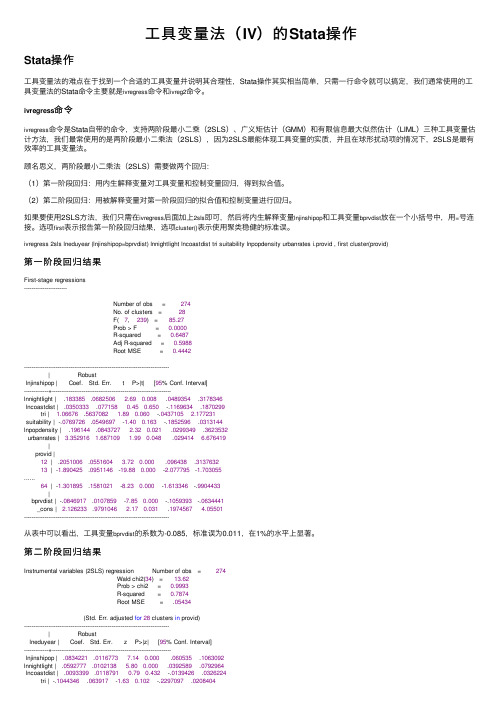
如果要使⽤2SLS⽅法,我们只需在ivregress后⾯加上2sls即可,然后将内⽣解释变量lnjinshipop和⼯具变量bprvdist放在⼀个⼩括号中,⽤=号连接。
选项first表⽰报告第⼀阶段回归结果,选项cluster()表⽰使⽤聚类稳健的标准误。
ivregress 2sls lneduyear (lnjinshipop=bprvdist) lnnightlight lncoastdist tri suitability lnpopdensity urbanrates i.provid , first cluster(provid)第⼀阶段回归结果First-stage regressions-----------------------Number of obs = 274No. of clusters = 28F( 7, 239) = 85.27Prob > F = 0.0000R-squared = 0.6487Adj R-squared = 0.5988Root MSE = 0.4442------------------------------------------------------------------------------| Robustlnjinshipop | Coef. Std. Err. t P>|t| [95% Conf. Interval]-------------+----------------------------------------------------------------lnnightlight | .183385 .0682506 2.690.008 .0489354 .3178346lncoastdist | .0350333 .0771580.450.650 -.1169634 .1870299tri | 1.06676 .5637082 1.890.060 -.0437105 2.177231suitability | -.0769726 .0549697 -1.400.163 -.1852596 .0313144lnpopdensity | .196144 .0843727 2.320.021 .0299349 .3623532urbanrates | 3.352916 1.687109 1.990.048 .029414 6.676419|provid |12 | .2051006 .0551604 3.720.000 .096438 .313763213 | -1.890425 .0951146 -19.880.000 -2.077795 -1.703055......64 | -1.301895 .1581021 -8.230.000 -1.613346 -.9904433|bprvdist | -.0846917 .0107859 -7.850.000 -.1059393 -.0634441_cons | 2.126233 .9791046 2.170.031 .1974567 4.05501------------------------------------------------------------------------------从表中可以看出,⼯具变量bprvdist的系数为-0.085,标准误为0.011,在1%的⽔平上显著。
高维回归stata工具变量法命令
高维回归stata工具变量法命令
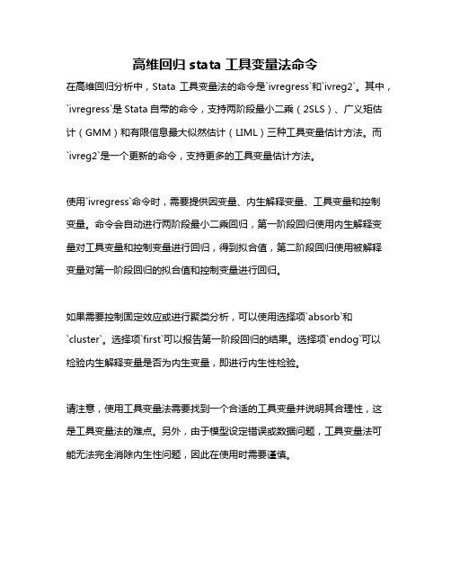
在高维回归分析中,Stata工具变量法的命令是`ivregress`和`ivreg2`。
其中,`ivregress`是Stata自带的命令,支持两阶段最小二乘(2SLS)、广义矩估计(GMM)和有限信息最大似然估计(LIML)三种工具变量估计方法。
而`ivreg2`是一个更新的命令,支持更多的工具变量估计方法。
使用`ivregress`命令时,需要提供因变量、内生解释变量、工具变量和控制变量。
命令会自动进行两阶段最小二乘回归,第一阶段回归使用内生解释变量对工具变量和控制变量进行回归,得到拟合值,第二阶段回归使用被解释变量对第一阶段回归的拟合值和控制变量进行回归。
如果需要控制固定效应或进行聚类分析,可以使用选择项`absorb`和
`cluster`。
选择项`first`可以报告第一阶段回归的结果。
选择项`endog`可以检验内生解释变量是否为内生变量,即进行内生性检验。
请注意,使用工具变量法需要找到一个合适的工具变量并说明其合理性,这是工具变量法的难点。
另外,由于模型设定错误或数据问题,工具变量法可能无法完全消除内生性问题,因此在使用时需要谨慎。
stata的u型关系工具变量法
stata的u型关系工具变量法Stata的u型关系工具变量法引言:在经济学和社会科学研究中,我们常常面临着因果关系的推断问题。
然而,由于自然实验的不可行性,我们无法直接观察到所有可能的结果。
为了解决这个问题,研究者们常常利用工具变量法来处理内生性问题。
本文将介绍Stata软件中的一种工具变量法——u型关系工具变量法,并讨论其应用和优势。
1. 工具变量法简介工具变量法是一种用来解决内生性问题的统计方法。
在经济学研究中,内生性指的是某个自变量与误差项之间存在相关关系,从而导致回归结果的偏误。
工具变量法的基本思想是利用一个或多个与内生变量高度相关但与误差项无关的变量作为“工具变量”,通过两阶段最小二乘法来估计内生变量的系数。
2. u型关系工具变量法在一些研究中,我们可能遇到自变量与因变量之间存在非线性关系的情况。
此时,传统的线性工具变量法可能无法有效地估计因果效应。
针对这种情况,Stata提供了一种u型关系工具变量法。
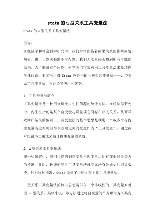
u型关系工具变量法的核心思想是引入一个非线性的工具变量来处理u型关系。
具体来说,该方法通过将自变量的平方项作为工具变量,来捕捉自变量与因变量之间的非线性关系。
这种方法可以有效地解决因果效应的非线性估计问题。
3. u型关系工具变量法的应用u型关系工具变量法在实证研究中有着广泛的应用。
以教育经济学为例,研究者常常关注教育水平对收入的影响,并希望探讨该关系是否存在非线性效应。
利用u型关系工具变量法,研究者可以更准确地估计教育水平对收入的因果效应,并得出更精确的结论。
u型关系工具变量法还可以应用于医学研究、环境经济学等领域。
在医学研究中,研究者可能对某种治疗方法对患者健康状况的影响感兴趣。
通过引入自变量的平方项作为工具变量,研究者可以更好地探究治疗方法对健康状况的非线性效应。
4. u型关系工具变量法的优势相比于传统的线性工具变量法,u型关系工具变量法具有以下几个优势:u型关系工具变量法可以更准确地估计因果效应。
STATA常用命令总结(34个含使用示例)
STATA常用命令总结(34个含使用示例)1. sum:计算变量的简要统计信息,如均值、标准差等。
示例:sum variable2. tabulate:生成变量的频数表。
示例:tabulate variable3. describe:显示数据集的基本信息,如变量名和数据类型。
示例:describe dataset4. drop:删除数据集中的变量。
示例:drop variable5. keep:保留数据集中的变量,删除其他变量。
示例:keep variable6. rename:重命名变量。
示例:rename variable newname7. gen:根据已有变量生成新的变量。
示例:gen newvar = expression8. egen:根据已有变量生成新的变量,可以使用更复杂的函数和运算符。
示例:egen newvar = function(variable)9. recode:对变量的取值进行重新编码。
示例:recode variable (oldvalues= newvalues) 10. dropif:根据条件删除观测。
示例:dropif condition11. keepif:根据条件保留观测。
示例:keepif condition12. sort:对数据集按指定变量进行排序。
示例:sort variable13. merge:将两个数据集按照共享变量合并。
示例:merge 1:1 variable using dataset214. reshape:将数据从宽格式转换为长格式或反之。
示例:reshape long var, i(id) j(year)15. regress:进行线性回归分析。
示例:regress dependent_var independent_vars 16. logistic:进行逻辑回归分析。
示例:logistic dependent_var independent_vars 17. probit:进行Probit回归分析。
STATA常用命令总结(34个含使用示例)

STATA常用命令总结(34个含使用示例)1. clear:清空当前工作空间中的数据。
示例:clear2. use:加载数据文件。
示例:use "data.dta"3. describe:查看数据文件的基本信息。
示例:describe4. summarize:统计数据的描述性统计量。
示例:summarize var1 var2 var35. tabulate:制作数据的列联表。
示例:tabulate var1 var26. scatter:绘制散点图。
示例:scatter x_var y_var7. histogram:绘制直方图。
示例:histogram var8. boxplot:绘制箱线图。
示例:boxplot var1 var29. ttest:进行单样本或双样本t检验。
示例:ttest var, by(group_var)10. regress:进行最小二乘法线性回归分析。
示例:regress dependent_var independent_var1 independent_var211. logistic:进行逻辑斯蒂回归分析。
示例:logistic dependent_var independent_var1 independent_var212. anova:进行方差分析。
示例:anova dependent_var independent_var13. chi2:进行卡方检验。
示例:chi2 var1 var214. correlate:计算变量之间的相关系数。
示例:correlate var1 var2 var315. replace:替换数据中的一些值。
示例:replace var = new_value if condition16. drop:删除变量或观察。
示例:drop var17. rename:重命名变量。
示例:rename old_var new_var18. generate:生成新变量。
- 1、下载文档前请自行甄别文档内容的完整性,平台不提供额外的编辑、内容补充、找答案等附加服务。
- 2、"仅部分预览"的文档,不可在线预览部分如存在完整性等问题,可反馈申请退款(可完整预览的文档不适用该条件!)。
- 3、如文档侵犯您的权益,请联系客服反馈,我们会尽快为您处理(人工客服工作时间:9:00-18:30)。
●本实例使用数据集“grilic.dta”。
●先看一下数据集的统计特征:
●考察智商与受教育年限的相关关系:
上表显示,智商(在一定程度上可以视为能力的代理变量)与受教育年限具有强烈的正相关关系(相关系数为0.51)。
●作为一个参考系,先进行OLS回归,并使用稳健标准差:
其中expr, tenure, rns, smsa均为控制变量,而我们主要感兴趣的是变量受教育年限(s)。
回归的结果显示,教育投资的年回报率为10.26%,这个似乎太高了。
可能的原因是,由于遗漏变量“能力”与受教育正相关,故“能力”对工资的贡献也被纳入教育的贡献,因此高估了教育的回报率。
●引入智商iq作为能力的代理变量,再进行OLS回归:
虽然教育的投资回报率有所下降,但是依然很高。
●由于用iq作为能力的代理变量有测量误差,故iq是内生变量,考虑使用变量(med(母亲的受教育年限)、kww(在“knowledge of the World of Work”中的成绩)、mrt(婚姻虚拟变量,已婚=1)age(年龄))作为iq的工具变量,进行2SLS回归,并使用稳健的标准差:
在此2SLS回归中,教育回报率反而上升到13.73%,而iq对工资的贡献居然为负值。
使用工具变量的前提是工具变量的有
效性。
为此,进行过度识别检验,考察是否所有的工具变量均外生,即与扰动项不相关:
结果强烈拒绝所有工具变量均外生的原假设。
●考虑仅使用变量(med, kww)作为iq的工具变量,再次进行2SLS回归,同时显示第一阶段的回归结果:
上表显示,教育的回报率为6.08%,较为合理,再次进行过度识别检验:
接受原假设,认为(med,kww)外生,与扰动项不相关。
●进一步考察有效工具变量的第二个条件,即工具变量与内生变量的相关性。
从第一阶段的回归结果可以看出,工具变量对内生变量具有较好的解释力。
更正式的检验如下:
从以上结果可以看出,虽然Shea’s partial R^2不到0.04,但是F统计量为13.40>10。
我们知道,虽然2SLS是一致的,但却是有偏的,故使用2SLS 会带来“显著性水平扭曲”(size distortion),而且这种扭曲随着弱工具变量而增大。
上表的最后部分显示,如果在结构方程中对内生解释变量的显著性进行“名义显著性水平”(nominal size)为5%的沃尔德检验,加入可以接受的“真实显著性水平”(true size)不超过15%,则可以拒绝“弱工具变量”的原假设,因为最小特征值统计量为14.91,大于临界值11.59。
总之我们有理由认为不存在弱工具变量。
但为了稳健起见,下面使用对弱工具变量更不敏感的有限信息最大似然法(LIML): 结果发现,LIML的系数估计值与2SLS非常接近,这也从侧面印证了“不存在弱工具变量”。
●使用工具变量法的前提是存在内生解释变量,为此须进行豪斯曼检验,其原假设是“所有的解释变量均为外生”:
上表显示,可以在5%的显著性水平下拒绝“所有解释变量均外生的原假设”,即认为存在内生解释变量iq。
由于传统的豪斯曼检验建立在同方差的前提下,故在上述回归中均没有使用稳健标准差。
●由于传统的豪斯曼检验在异方差的情形下不成立,下面使用异方差稳健的DWH检验:
据此可认为iq为内生解释变量。
●如果存在异方差,则GMM比2SLS更有效。
为此进行如下的最优GMM估计:
●进行过度识别检验:
●由于p值为0.70,故认为所有的工具变量均为外生。
考虑迭代GMM:
●如果希望将以上各种估计法的系数估计值及其标准差列在同一张表中,可使用如下命令:
●。