A COMPONENT BASED PRIMAL DUAL APPROACH

合集下载

运筹学英汉词汇ABC

运筹学英汉词汇(0,1) normalized ――0-1规范化Aactivity ――工序additivity――可加性adjacency matrix――邻接矩阵adjacent――邻接aligned game――结盟对策analytic functional equation――分析函数方程approximation method――近似法arc ――弧artificial constraint technique ――人工约束法artificial variable――人工变量augmenting path――增广路avoid cycle method ――避圈法Bbackward algorithm――后向算法balanced transportation problem――产销平衡运输问题basic feasible solution ――基本可行解basic matrix――基阵basic solution ――基本解basic variable ――基变量basic ――基basis iteration ――换基迭代Bayes decision――贝叶斯决策big M method ――大M 法binary integer programming ――0-1整数规划binary operation――二元运算binary relation――二元关系binary tree――二元树binomial distribution――二项分布bipartite graph――二部图birth and death process――生灭过程Bland rule ――布兰德法则branch node――分支点branch――树枝bridge――桥busy period――忙期Ccapacity of system――系统容量capacity――容量Cartesian product――笛卡儿积chain――链characteristic function――特征函数chord――弦circuit――回路coalition structure――联盟结构coalition――联盟combination me――组合法complement of a graph――补图complement of a set――补集complementary of characteristic function――特征函数的互补性complementary slackness condition ――互补松弛条件complementary slackness property――互补松弛性complete bipartite graph――完全二部图complete graph――完全图completely undeterministic decision――完全不确定型决策complexity――计算复杂性congruence method――同余法connected component――连通分支connected graph――连通图connected graph――连通图constraint condition――约束条件constraint function ――约束函数constraint matrix――约束矩阵constraint method――约束法constraint ――约束continuous game――连续对策convex combination――凸组合convex polyhedron ――凸多面体convex set――凸集core――核心corner-point ――顶点（角点）cost coefficient――费用系数cost function――费用函数cost――费用criterion ; test number――检验数critical activity ――关键工序critical path method ――关键路径法（CMP ）critical path scheduling ――关键路径cross job ――交叉作业curse of dimensionality――维数灾customer resource――顾客源customer――顾客cut magnitude ――截量cut set ――截集cut vertex――割点cutting plane method ――割平面法cycle ――回路cycling ――循环Ddecision fork――决策结点decision maker决――策者decision process of unfixed step number――不定期决策过程decision process――决策过程decision space――决策空间decision variable――决策变量decision决－－策decomposition algorithm――分解算法degenerate basic feasible solution ――退化基本可行解degree――度demand――需求deterministic inventory model――确定贮存模型deterministic type decision――确定型决策diagram method ――图解法dictionary ordered method ――字典序法differential game――微分对策digraph――有向图directed graph――有向图directed tree――有向树disconnected graph――非连通图distance――距离domain――定义域dominate――优超domination of strategies――策略的优超关系domination――优超关系dominion――优超域dual graph――对偶图Dual problem――对偶问题dual simplex algorithm ――对偶单纯形算法dual simplex method――对偶单纯形法dummy activity――虚工序dynamic game――动态对策dynamic programming――动态规划Eearliest finish time――最早可能完工时间earliest start time――最早可能开工时间economic ordering quantity formula――经济定购批量公式edge ――边effective set――有效集efficient solution――有效解efficient variable――有效变量elementary circuit――初级回路elementary path――初级通路elementary ――初等的element――元素empty set――空集entering basic variable ――进基变量equally liability method――等可能性方法equilibrium point――平衡点equipment replacement problem――设备更新问题equipment replacing problem――设备更新问题equivalence relation――等价关系equivalence――等价Erlang distribution――爱尔朗分布Euler circuit――欧拉回路Euler formula――欧拉公式Euler graph――欧拉图Euler path――欧拉通路event――事项expected value criterion――期望值准则expected value of queue length――平均排队长expected value of sojourn time――平均逗留时间expected value of team length――平均队长expected value of waiting time――平均等待时间exponential distribution――指数分布external stability――外部稳定性Ffeasible basis ――可行基feasible flow――可行流feasible point――可行点feasible region ――可行域feasible set in decision space――决策空间上的可行集feasible solution――可行解final fork――结局结点final solution――最终解finite set――有限集合flow――流following activity ――紧后工序forest――森林forward algorithm――前向算法free variable ――自由变量function iterative method――函数迭代法functional basic equation――基本函数方程function――函数fundamental circuit――基本回路fundamental cut-set――基本割集fundamental system of cut-sets――基本割集系统fundamental system of cut-sets――基本回路系统Ggame phenomenon――对策现象game theory――对策论game――对策generator――生成元geometric distribution――几何分布goal programming――目标规划graph theory――图论graph――图HHamilton circuit――哈密顿回路Hamilton graph――哈密顿图Hamilton path――哈密顿通路Hasse diagram――哈斯图hitchock method ――表上作业法hybrid method――混合法Iideal point――理想点idle period――闲期implicit enumeration method――隐枚举法in equilibrium――平衡incidence matrix――关联矩阵incident――关联indegree――入度indifference curve――无差异曲线indifference surface――无差异曲面induced subgraph――导出子图infinite set――无限集合initial basic feasible solution ――初始基本可行解initial basis ――初始基input process――输入过程Integer programming ――整数规划inventory policy―v存贮策略inventory problem―v货物存储问题inverse order method――逆序解法inverse transition method――逆转换法isolated vertex――孤立点isomorphism――同构Kkernel――核knapsack problem ――背包问题Llabeling method ――标号法latest finish time――最迟必须完工时间leaf――树叶least core――最小核心least element――最小元least spanning tree――最小生成树leaving basic variable ――出基变量lexicographic order――字典序lexicographic rule――字典序lexicographically positive――按字典序正linear multiobjective programming――线性多目标规划Linear Programming Model――线性规划模型Linear Programming――线性规划local noninferior solution――局部非劣解loop method――闭回路loop――圈loop――自环（环）loss system――损失制Mmarginal rate of substitution――边际替代率Marquart decision process――马尔可夫决策过程matching problem――匹配问题matching――匹配mathematical programming――数学规划matrix form ――矩阵形式matrix game――矩阵对策maximum element――最大元maximum flow――最大流maximum matching――最大匹配middle square method――平方取中法minimal regret value method――最小后悔值法minimum-cost flow――最小费用流mixed expansion――混合扩充mixed integer programming ――混合整数规划mixed Integer programming――混合整数规划mixed Integer ――混合整数规划mixed situation――混合局势mixed strategy set――混合策略集mixed strategy――混合策略mixed system――混合制most likely estimate――最可能时间multigraph――多重图multiobjective programming――多目标规划multiobjective simplex algorithm――多目标单纯形算法multiple optimal solutions ――多个最优解multistage decision problem――多阶段决策问题multistep decision process――多阶段决策过程Nn- person cooperative game ――n人合作对策n- person noncooperative game――n人非合作对策n probability distribution of customer arrive――顾客到达的n 概率分布natural state――自然状态nature state probability――自然状态概率negative deviational variables――负偏差变量negative exponential distribution――负指数分布network――网络newsboy problem――报童问题no solutions ――无解node――节点non-aligned game――不结盟对策nonbasic variable ――非基变量nondegenerate basic feasible solution――非退化基本可行解nondominated solution――非优超解noninferior set――非劣集noninferior solution――非劣解nonnegative constrains ――非负约束non-zero-sum game――非零和对策normal distribution――正态分布northwest corner method ――西北角法n-person game――多人对策nucleolus――核仁null graph――零图Oobjective function ――目标函数objective( indicator) function――指标函数one estimate approach――三时估计法operational index――运行指标operation――运算optimal basis ――最优基optimal criterion ――最优准则optimal solution ――最优解optimal strategy――最优策略optimal value function――最优值函数optimistic coefficient method――乐观系数法optimistic estimate――最乐观时间optimistic method――乐观法optimum binary tree――最优二元树optimum service rate――最优服务率optional plan――可供选择的方案order method――顺序解法ordered forest――有序森林ordered tree――有序树outdegree――出度outweigh――胜过Ppacking problem ――装箱问题parallel job――平行作业partition problem――分解问题partition――划分path――路path――通路pay-off function――支付函数payoff matrix――支付矩阵payoff――支付pendant edge――悬挂边pendant vertex――悬挂点pessimistic estimate――最悲观时间pessimistic method――悲观法pivot number ――主元plan branch――方案分支plane graph――平面图plant location problem――工厂选址问题player――局中人Poisson distribution――泊松分布Poisson process――泊松流policy――策略polynomial algorithm――多项式算法positive deviational variables――正偏差变量posterior――后验分析potential method ――位势法preceding activity ――紧前工序prediction posterior analysis――预验分析prefix code――前级码price coefficient vector ――价格系数向量primal problem――原问题principal of duality ――对偶原理principle of optimality――最优性原理prior analysis――先验分析prisoner’s dilemma――囚徒困境probability branch――概率分支production scheduling problem――生产计划program evaluation and review technique――计划评审技术(PERT) proof――证明proper noninferior solution――真非劣解pseudo-random number――伪随机数pure integer programming ――纯整数规划pure strategy――纯策略Qqueue discipline――排队规则queue length――排队长queuing theory――排队论Rrandom number――随机数random strategy――随机策略reachability matrix――可达矩阵reachability――可达性regular graph――正则图regular point――正则点regular solution――正则解regular tree――正则树relation――关系replenish――补充resource vector ――资源向量revised simplex method――修正单纯型法risk type decision――风险型决策rooted tree――根树root――树根Ssaddle point――鞍点saturated arc ――饱和弧scheduling (sequencing) problem――排序问题screening method――舍取法sensitivity analysis ――灵敏度分析server――服务台set of admissible decisions(policies) ――允许决策集合set of admissible states――允许状态集合set theory――集合论set――集合shadow price ――影子价格shortest path problem――最短路线问题shortest path――最短路径simple circuit――简单回路simple graph――简单图simple path――简单通路Simplex method of goal programming――目标规划单纯形法Simplex method ――单纯形法Simplex tableau――单纯形表single slack time ――单时差situation――局势situation――局势slack variable ――松弛变量sojourn time――逗留时间spanning graph――支撑子图spanning tree――支撑树spanning tree――生成树stable set――稳定集stage indicator――阶段指标stage variable――阶段变量stage――阶段standard form――标准型state fork――状态结点state of system――系统状态state transition equation――状态转移方程state transition――状态转移state variable――状态变量state――状态static game――静态对策station equilibrium state――统计平衡状态stationary input――平稳输入steady state――稳态stochastic decision process――随机性决策过程stochastic inventory method――随机贮存模型stochastic simulation――随机模拟strategic equivalence――策略等价strategic variable, decision variable ――决策变量strategy (policy) ――策略strategy set――策略集strong duality property ――强对偶性strong ε-core――强ε-核心strongly connected component――强连通分支strongly connected graph――强连通图structure variable ――结构变量subgraph――子图sub-policy――子策略subset――子集subtree――子树surplus variable ――剩余变量surrogate worth trade-off method――代替价值交换法symmetry property ――对称性system reliability problem――系统可靠性问题Tteam length――队长tear cycle method――破圈法technique coefficient vector ――技术系数矩阵test number of cell ――空格检验数the branch-and-bound technique ――分支定界法the fixed-charge problem ――固定费用问题three estimate approach一―时估计法total slack time――总时差traffic intensity――服务强度transportation problem ――运输问题traveling salesman problem――旅行售货员问题tree――树trivial graph――平凡图two person finite zero-sum game二人有限零和对策two-person game――二人对策two-phase simplex method ――两阶段单纯形法Uunbalanced transportation problem ――产销不平衡运输问题unbounded ――无界undirected graph――无向图uniform distribution――均匀分布unilaterally connected component――单向连通分支unilaterally connected graph――单向连通图union of sets――并集utility function――效用函数Vvertex――顶点voting game――投票对策Wwaiting system――等待制waiting time――等待时间weak duality property ――弱对偶性weak noninferior set――弱非劣集weak noninferior solution――弱非劣解weakly connected component――弱连通分支weakly connected graph――弱连通图weighed graph ――赋权图weighted graph――带权图weighting method――加权法win expectation――收益期望值Zzero flow――零流zero-sum game――零和对策zero-sum two person infinite game――二人无限零和对策。

集合覆盖问题的模型与算法（PDF）

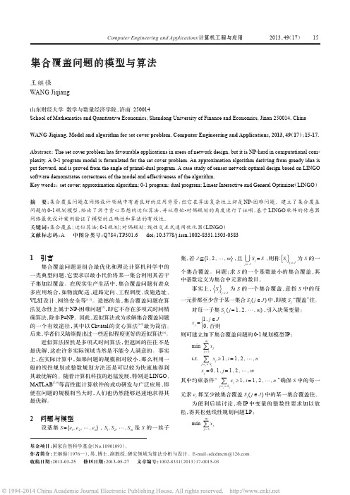
2013，49（17）1引言集合覆盖问题是组合最优化和理论计算机科学中的一类典型问题，它要求以最小代价将某一集合利用其若干子集加以覆盖。

在现实生产生活中，集合覆盖问题有着众多应用场合，如物流配送、道路定向、工程调度、设施选址、VLSI 设计、网络安全等[1-2]。

遗憾的是，集合覆盖问题在算法复杂性上属于NP-困难问题[3]，即它不存在多项式时间精确算法，除非P=NP 。

因此，近似算法成为求解集合覆盖问题的一个有效途径，其中以Chvátal 的贪心算法[4-5]最为简洁。

后来，学者们又陆续提出过一些近似程度更好的近似算法[6]。

近似算法固然是多项式时间算法，但返回的往往不是最优解，这在许多实际领域当然是不能令人满意的。

事实上，在实际计算中，如果问题的规模相对较小，那么利用一般的线性规划或整数规划方法还是可以较为快速地得到其最优解的。

随着计算机科技的迅猛发展，特别是LINGO 、MATLAB [7-9]等高性能计算软件的成功研发与广泛应用，即便在问题的规模相当大时，人们也仍然能够迅速地求得其最优解。

2问题与模型设基集S ={e 1 e 2 e n }，S 1 S 2 S m 是S 的一族子集，若J Í{1 2 m }，且j ÎJS j =S ，则称{}S j j ÎJ为S 的一个集合覆盖。

问题：求S 的一个基数最小的集合覆盖，其中基数定义为集合中元素的数目。

事实上，{}S jj ÎJ为S 的一个集合覆盖，意指S 中的每一元素都至少含于某一集合S j (j ÎJ )中，即被S j“覆盖”住。

对每一子集S j (j =1 2 m )，引入决策变量：x j ={1 j ÎJ0 否则则可建立如下集合覆盖问题的0-1规划模型IP ：min åj =1mx j s.t.åj :e i ÎS jx j 1 i =1 2 nx j =0 1 j =1 2 m其中约束条件“åj :e i ÎS jx j 1 i =1 2 n ”确保S 中的每一元素e i 都至少被集合覆盖S j (j ÎJ )中的某一集合覆盖住。

primal-dual-based method

primal-dual-based method头部航程规划问题（Primal-Dual based method）引言：头部航程规划问题是一种常见的优化问题，它的目标是在给定航线网络和航线容量的情况下，找到一种合理的飞行计划，以最小化总飞行成本并满足航线容量限制。

这个问题在航空运输管理中具有重要的实际意义。

本文将介绍一种基于Primal-Dual方法的解决方案，解释其原理和应用。

第一部分：问题描述在头部航程规划问题中，我们考虑一个航线网络G=(V, E)，其中V是航线节点的集合，E是连接这些节点的航线的集合。

每条航线e属于E都有一个容量限制Ce，表示该航线能够承载的最大飞行量。

同时，每条航线e 可以有一个飞行成本Ce，表示单位距离的运营成本。

我们的目标是找到一种最优的头部航程规划方案，以最小化总飞行成本，并且满足航线容量限制。

第二部分：Primal-Dual算法简介Primal-Dual算法是一种常用的解决线性规划问题的方法，它将原问题转化为对偶问题，并通过不断调整原问题和对偶问题之间的关系，逐步找到最优解。

在头部航程规划问题中，我们可以将其转化为一个线性规划问题，然后应用Primal-Dual算法求解。

第三部分：Primal-Dual算法的步骤1. 初始化：- 将所有航线的飞行量设置为0，即x_e=0，这意味着初始航程规划方案中没有航线被使用。

- 创建对偶变量p_v，表示每个节点的流平衡。

初始化为0。

2. 进入迭代过程：- 根据当前航线规划方案（即飞行量x_e）计算对偶变量p_v。

这可以通过使用Bellman-Ford算法来计算最短路径和对应的费用，将费用作为对偶变量p_v。

- 根据对偶变量p_v，计算每条航线的费用约束，即c_e = Ce - p_u + p_v，其中u和v是航线e的起始节点和终止节点。

- 利用线性规划方法求解最小费用流问题，即最小化目标函数Σ_c_e*x_e，同时满足容量约束Σ_x_e≤Ce，其中x_e是航线e的飞行量。

The primal-dual method for approximation algorithms and its application to network design p

1
Introduction
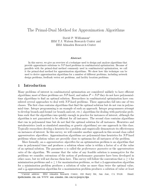
Many problems of interest in combinatorial optimization are considered unlikely to have eﬃcient algorithms; most of these problems are N P -hard, and unless P = N P they do not have polynomialtime algorithms to ﬁnd an optimal solution. Researchers in combinatorial optimization have considered several approaches to deal with N P -hard problems. These approaches fall into one of two classes. The ﬁrst class contains algorithms that ﬁnd the optimal solution but do not run in polynomial time. Integer programming is an example of such an approach. Integer programmers attempt to develop branch-and-bound (or branch-and-cut, etc.) algorithms for dealing with particular problems such that the algorithm runs quickly enough in practice for instances of interest, although the algorithm is not guaranteed to be eﬃcient for all instances. The second class contains algorithms that run in polynomial time but do not ﬁnd the optimal solution for all instances. Heuristics and metaheuristics (such as simulated annealing or genetic algorithms) are one approach in this class. Typically researchers develop a heuristic for a problem and empirically demonstrate its eﬀectiveness on instances of interest. In this survey, we will consider another approach in this second class called approximation algorithms. Approximation algorithms are polynomial-time heuristics for N P -hard problems whose solution values are provably close to optimum for all instances of the problem. More formally, an α-approximation algorithm for an optimization problem is an algorithm that runs in polynomial time and produces a solution whose value is within a factor of α of the value of an optimal solution. The parameter α is called the performance guarantee or the approximation ratio of the algorithm. We assume that the value of any feasible solution is nonnegative for the problems we consider; extensions of the notion of performance guarantee have been developed in other cases, but we will not discuss them here. This survey will follow the convention that α ≥ 1 for minimization problems and α ≤ 1 for maximization problems, so that a 2-approximation algorithm for a minimization problem produces a solution of value no more than twice the optimal value, 1 and a 2 -approximation algorithm for a maximization problem produces a solution of value at least

本福特定律的原理概述

本福特定律的原理概述The principle of the Ford Duality Law is a fundamental concept in mathematics and physics. It deals with the relationship between primal and dual feasible solutions in linear programming. The law states that if a primal linear program has an optimal solution, then its dual linear program will also have an optimal solution, and the optimal values of the two solutions will be equal.福特定律的原理对数学和物理学都有重要影响。

它涉及线性规划中原问题和对偶问题之间的关系。

定律表明，如果原线性规划有最优解，则其对偶线性规划也将有最优解，并且两个最优解的值将相等。

The duality principle serves as a powerful tool in optimization theory and is crucial for understanding the underlying structure of linear programming problems. By relating the primal and dual problems, it allows us to make inferences about one problem based on the solutions of the other. This duality relationship provides insight into the nature of constraints and objectives in a linear programming model.对偶原理是优化理论中的重要工具，对于理解线性规划问题的基本结构至关重要。

primaldual函数关系

primaldual函数关系Primal-dual is a powerful optimization technique used to solve linear programming problems. It is based on the principle of duality from convex analysis and provides a way toefficiently solve a primal problem by solving its dual problem simultaneously.The primal problem is typically a minimization problem with linear constraints, while the dual problem is a maximization problem with linear constraints. The primal-dual technique constructs the dual problem from the primal problem and uses their relationship to solve both problems together.The primal-dual approach starts with the primal problem, which can be written as:minimize c^T xsubject to Ax = band x >= 0where c is the cost vector, x is the variable vector, A is the constraint matrix, and b is the constraint vector.To construct the dual problem, we introduce a dual variable y for each constraint in the primal problem. The dual problem can then be written as:maximize b^T ysubject to A^T y <= cand y >= 0where y is the dual variable vector.The primal and dual problems are said to be dual to each other, as they are linked through the following fundamental properties:1. The primal problem seeks to minimize the objective function subject to the constraints, while the dual problem seeks to maximize the objective function subject to its own set of constraints.2. The optimal solution to the primal problem provides a lower bound for the optimal solution to the dual problem, and vice versa. This is known as the weak duality property.The primal-dual technique exploits these properties to iteratively improve the solutions of both the primal and dual problems until convergence is reached. This is done by updating the dual variables based on the current primal solution, andvice versa, until an optimal solution is found for both problems.In conclusion, the primal-dual technique is a powerful optimization approach that allows for the simultaneous solution of the primal and dual problems. It provides a way toefficiently solve linear programming problems and offersinsights into the relationship between the primal and dualproblems. By exploiting the properties of duality, the primal-dual technique provides a powerful tool for solving large-scale optimization problems.。

The Primal-Dual Algorithm(原始对偶优化算法)

Ax = b ≥ 0 x≥0
Dual max w = π′b
π′A ≤ c′ π′ ≷ 0
Assume b ≥ 0 and we know dual feasible π.
Recall that x, π are jointly optimal iff they satisfy
∀i, πi(a′ix − bi) = 0 and ∀j, (cj − π′Aj)xj = 0.
cj − π′Aj π¯′Aj
The new cost is
w∗ = π′b + θ1π¯′b = w + θ1π¯′b > w.
11
procedure primal-dual begin
infeasible := ‘no’, opt := ‘no’; let π be feasible in D while infeasible =‘no’ and opt =‘no’ do begin set J = {j : π′Aj = cj};
8
Dual max w = π′b
π′A ≤ c′ π′ ≷ 0
J = {j : π′Aj = cj} π is feasible
DRP max w = π′b
π′Aj ≤ 0 j ∈ J πi ≤ 1 i ≤ m πi ≷ 0
π¯ is optimal
We “improve” cost of π by setting π∗ = π + θπ¯, θ > 0.
10
Dual max w = π′b
π′A ≤ c′ π′ ≷ 0
J = {j : π′Aj = cj} π is feasible
DRP max w = π′b

primal-dual-based method -回复

primal-dual-based method -回复什么是原始对偶法方法（primal-dual-based method）？原始对偶法方法是一种优化算法，用于求解具有原始对偶结构的优化问题。

在这种方法中，优化问题被分解成原始问题和对偶问题，并通过迭代地求解它们之间的对偶性关系来获得最优解。

原始对偶法方法的一般框架如下：1.确定原始问题：将给定的优化问题表达为其原始形式，并定义目标函数和约束条件。

原始问题通常是一个最小化问题，其目标函数为要最小化的目标值。

2.确定对偶问题：通过定义对偶变量和对偶约束来构造对偶问题。

对偶问题通常是一个最大化问题，其目标函数是原始问题的拉格朗日对偶函数。

3.建立对偶性关系：根据原始问题和对偶问题之间的对偶性关系，构建一个线性方程系统。

4.迭代求解：通过迭代地更新原始变量和对偶变量来求解原始问题和对偶问题。

在每次迭代中，通过将原始变量和对偶变量向梯度下降方向更新，逐渐向最优解逼近。

5.停止准则：定义一个停止准则，用于判断迭代是否收敛。

常用的停止准则包括目标函数值的变化或对偶变量的变化小于某个阈值。

下面以一个具体的优化问题来说明原始对偶法方法的应用。

假设我们有一个线性规划问题，即最小化目标函数f(x) = c^T x，其中x 是一个n 维向量，满足线性约束Ax = b，其中A 是一个m×n 的矩阵，b 是一个m 维向量。

我们可以将该线性规划问题分解为原始问题和对偶问题。

原始问题：最小化f(x) = c^T x约束条件Ax = b对偶问题：最大化g(y) = b^T y约束条件A^T y + s = c，其中s 是一个n 维向量，称为松弛变量。

我们可以根据原始问题和对偶问题之间的对偶性关系，建立一个线性方程系统。

对于原始问题，我们可以使用梯度下降法进行迭代求解。

在每次迭代中，根据梯度下降方向更新原始变量x，直到满足停止准则。

对于对偶问题，我们可以使用梯度上升法进行迭代求解。

KSC

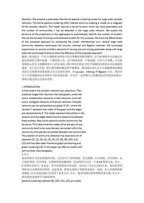
Abstract—We propose a parameter-free kernel spectral clustering model for large scale complex networks. The kerne spectral clustering (KSC) method works by creating a model on a subgraph of the complex network. The model requires a kernel function which can have parameters and the number of communities k has be detected in the large scale network. We exploit the structure of the projections in the eigenspace to automatically identify the number of clusters. We use the concept of entropy and balanced clusters for this purpose. We show the effectiveness of the proposed approach by comparing the cluster memberships w.r.t. several large scale community detection techniques like Louvain, Infomap and Bigclam methods. We conducted experiments on several synthetic networks of varying size and mixing parameter along with large scale real world experiments to show the efﬁciency of the proposed approach.摘要：我们提出一个在大规模复杂网络中的无参数核谱聚类模型。

项目进度管理研究综述

项目进度管理研究综述发表时间：2014-12-26T13:02:33.560Z 来源：《价值工程》2014年第11月上旬供稿作者：潘广钦[导读] 项目进度管理作为项目管理三大核心部分之一，是项目各利益方最为关注的内容，对项目成功与否起着决定性的作用，尤其是工期特别紧的项目潘广钦PAN Guang-qin（达州职业技术学院，达州635001）（Dazhou Vocational and Technical College，Dazhou 635001，China）摘要院项目进度管理作为项目管理的核心内容，直接决定着项目管理的成效。

本文在综合国内外项目进度管理研究成果的基础上，就关键链技术在项目进度管理中的必要性和意义进行了研究和探讨。

Abstract院As the core content of project management, project schedule management directly decides the effect of project management.Based on the research achievements of project schedule management at home and abroad, the necessity and significance of critical chaintechnology in project schedule management are studied and discussed.关键词院项目管理；项目进度管理；研究意义；综述Key words院project management；project schedule management；research significance；review中图分类号院TU723 文献标识码院A 文章编号院1006-4311（2014）31-0086-040 引言近年来，随着项目管理技术的不断发展成熟，项目进度管理作为其重要组成之一，也引发了一系列热议。

于慧敏，浙江大学，教授,博士生导师。主要研究方向为图像视频处理与

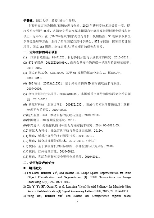
于慧敏，浙江大学，教授,博士生导师。

主要研究方向为图像/视频处理与分析。

2003年获科学技术三等奖一项，授权发明专利近20项，多篇论文发表在模式识别和计算机视觉领域顶尖学报和会议上。

近年来，在 (3D/2D)视频/图象处理与分析、视频监控、3D视频获取和医学图像处理等方面，主持了多项国家自然科学基金、973子课题、国家国防计划项目、国家863课题、浙江省重大/重点项目的研究和开发。

一、近年主持的科研项目(1)国家自然基金，61471321、目标协同分割与识别技术的研究、2015-2018。

(2) 973子课题，2012CB316406-1、面向公共安全的跨媒体呈现与验证和示范平、2012-2016。

(3)国家自然基金，60872069、基于3D 视频的运动分割与3D 运动估计、2009-2011。

(4) 863项目，2007AA01Z331、基于异构结构的3D实时获取技术与系统、2007-2009。

(5)浙江省科技计划项目，2013C310035 、多国纸币序列号和特殊污染字符识别技、2013-2015。

(6)浙江省科技计划重点项目, 2006C21035 、集成化多模医学影像信息计算和处理平台的研发、2006-2008。

(7)航天基金，***三维动目标的获取与重建、2008-2010。

(8)中国电信，3D视频监控系统、2010。

(9)中兴通讯，跨摄像机的目标匹配与跟踪技术研究、2014.05-2015.05。

(10)浙江大力科技，激光雷达导航与图像读表系统、2015-。

(11)横向，纸币序列号的实时识别技术、2011-2012。

(12)横向，清分机视频处理技术、2010-2012。

（参与）(13)横向，基于多摄像机的目标跟踪、事件检测与行为分析、2010。

(14)横向，红外视频雷达、2010-2012。

(15)横向，客运车辆行车安全视频分析系统、2010-2011。

二、近五年发表的论文期刊论文：1)Fei Chen, Huimin Yu#, and Roland Hu. Shape Sparse Representation for JointObject Classification and Segmentation [J]. IEEE Transactions on Image Processing 22(3): 992-1004 ,2013.2)Xie Y, Yu H#, Gong X, et al. Learning Visual-Spatial Saliency for Multiple-ShotPerson Re-Identification[J].Signal Processing Letters IEEE, 2015, 22:1854-1858.3)Yang, Bai, Huimin Yu#, and Roland Hu. Unsupervised regions basedsegmentation using object discovery, Journal of Visual Communication and Image Representation, 2015,31: 125-137.4)Fei Chen, Roland Hu, Huimin Yu#, Shiyan Wang: Reduced set density estimatorfor object segmentation based on shape probabilistic representation. J. Visual Communication and Image Representation,2012, 23(7): 1085-1094.5)Fei Chen, Huimin Yu#, Jincao Yao , Roland Hu ,Robust sparse kernel densityestimation by inducing randomness[J]，Pattern Analysis and Applications: Volume 18, Issue 2 (2015), Page 367-375.6)赵璐，于慧敏#，基于先验形状信息和水平集方法的车辆检测，浙江大学学报（工学版），pp.124-129,2010.1。

改进正则项的图像盲恢复方法

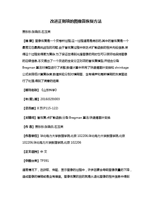
改进正则项的图像盲恢复方法贾彤彤;张晓乐;石玉英【摘要】图像恢复是一个反卷积过程,这一过程通常是病态的,其中的盲恢复是一个最常见也最具挑战性的问题.由于盲恢复过程中缺乏点扩散函数的相关先验信息,使得这个过程变得更为复杂.为了保证在得到光滑图像的同时也可以很好地保持图像的边缘信息,本文提出了一个改进的全变分正则项的盲恢复模型,并结合分裂Bregman算法对模型进行了求解.数值计算中采用了快速傅里叶变换和shrinkage 公式来降低计算复杂度.数值实验分别对模糊图、含有噪声和高斯模糊的灰度图进行了处理,得到了满意的结果.【期刊名称】《山东科学》【年(卷),期】2016(029)003【总页数】8页(P115-122)【关键词】盲恢复;点扩散函数;分裂Bregman算法;快速傅里叶变换【作者】贾彤彤;张晓乐;石玉英【作者单位】华北电力大学数理学院,北京102206;华北电力大学数理学院,北京102206;华北电力大学数理学院,北京102206【正文语种】中文【中图分类】TP391通常情况下，在获取、传输、显示图像的过程中，许多因素会导致图像质量的下降，造成图像的模糊或是含有噪音。

图像恢复的目的就是从退化图像的相关信息中得到尽可能接近原始图像的数据，从而恢复图像的本来面目，它在科学的各个领域都发挥着非常重要的作用[1-3]。

在图像处理中，原始图像与观测图像之间的关系可以表达如下：这里g代表退化图像，n是噪声。

A是模糊算子(也称为点扩散函数(PSF))，且A=h*u，h是紧凑的卷积核(如：高斯卷积核)，*表示卷积。

一般来说，由于模糊的过程很难得到，这使得PSF很难确定。

因此我们只能在缺乏PSF的先验信息的情况下，从观测到的图像g中提取一些有用的信息来得到恢复图像u，这一过程就称为图像盲恢复。

它的优点是在没有任何图像退化的先验知识的情况下也可以实现图像恢复过程。

反卷积过程中的病态特性，是反问题本身固有的一种特征。

图论可达性

摘要/介绍两种分别描述城市空间的度量结构和拓扑结构的图论表示法以及4种“图论可达性”指标，并以北京旧城的一个局部为案例来说明这4种可达性度量对于城市设计的作用和意义。

关键词/城市空间可达性图论可达性邻近中心度空间整合度空间句法重力可达性模型场所句法北京旧城图论可达性ABSTRACT/ This article aims to introduce two types of graph representations of urban space and four graph-theory accessibility indices, and demonstrate how these methods can assistarchitectural and urban design practise, based on a case study of aprecinct in the Old City of Beijing.KEY WO RDS/ urban space, accessibilit y, graph-theory accessibility, closeness centrality, spatial integration, space syntax, gravity-based accessibility, place syntax, the O ld City of Beijing英国建筑学家爱丽森・史密斯森和彼得・史密斯森夫妇(Alison Smithson & Peter Smithson)提出了“被充实的空”(The Charged Void)的概念，用以描述建成环境所赋予城市空间的活力。

他们认为：“建筑具有一种潜力可以使其周围的空间充满能量(energy)。

这种能量可以和其他形式的能量相融合，从而定义了空间中可能出现的各种活动和事件。

我们能够感知这一潜力的存在并且据此而行动，但却难以对这一潜力进行描述或者记录。

复杂网络理论在城市交通网络分析中的应用_赵月

1 ∑C 。 i N i∈G
节点 i 的聚类系数也可定义为： Ci = 包含节点 i 的三角形的个数以节点 i 为中心的三点组的个数， (4)
Eglobal =
1
N(N -1) i, j∈G, i≠j
∑εij =
1
N(N -1) i, j∈G, i≠j dij
∑
1
。
(5)
式中：以节点 i 为中心的三点组是指包括节点 i 的 3 个节点，并且至少存在从节点 i 到其他 2 个节点的 2 条边，如图 1 所示。根据式 (4) 可得：图 1(a) 中节点 i 的聚类系数
∑ ， ki(ki -1) l, m∈G, l≠m dlm
1
式中：dlm为子图 Gi中节点 l 和 m 间的最短路径长度。
1.5 集中性(Centrality)
集中性指标是一系列指标的集合，可用来衡量节点在网络中的地位。通过对复杂网络集中性指标的计算能够在规模庞大、结构复杂的网络中迅速地发现集中节点。对于不同的网络，需要用不同的指标来衡量其集中性，典型的集中性指标包括度指标 (Degree centrality)、紧密度指标 (Closeness centrality)、介数指标 (Betweenness centrality)、信息集中性指标 (Information centrality) 等，指标的具体计算方法可参照文献 [14~15]。
式中：N 为网络节点数。网络的平均路径长度也称为网络的特征路径长度，用来衡量网络节点间的离散程度。研究表明，尽管许多实际网络的节点数巨大，但网络的平均路径长度 L 相对于 N 来说却很小，这种现象称之为“小世界效应”[1]。

primal-dual 原始对偶算法

primal-dual 原始对偶算法一、概述Primal-Dual算法是一种用于解决复杂优化问题的算法，尤其在机器学习、统计学习、物流工程等领域有着广泛的应用。

该算法基于原始-对偶问题的思路，通过交替优化原始变量和其对偶变量，最终达到全局最优解。

二、算法原理Primal-Dual算法的基本思想是将原问题转化为一系列对偶问题，通过交替优化原始变量和其对偶变量，最终达到全局最优解。

具体步骤如下：1. 初始化：选择一个初始点作为原始变量的近似解，以及一个初始的解空间。

2. 迭代：在每次迭代中，根据当前解空间，求解对偶问题并更新对偶变量。

同时，根据对偶问题的解更新原始变量的近似解。

3. 终止条件：当满足终止条件（如达到最大迭代次数或解的改变小于预设阈值）时，算法停止。

算法的核心在于通过交替优化原始变量和其对偶变量，逐渐逼近原始问题的最优解。

具体来说，通过求解对偶问题，可以找到与原始问题解空间相关的潜在优化方向，进而通过原始-对偶变量的交替更新，逐渐逼近最优解。

三、算法步骤1. 初始化：选择一个初始点作为原始变量的近似解，以及一个初始的解空间。

2. 迭代：a. 对原始变量进行优化：求解原始问题的对偶问题，得到当前对偶变量的近似解。

根据对偶问题的解，更新原始变量的近似解。

b. 对对偶变量进行优化：根据更新后的原始变量的近似解，重新构造原始问题，并求解原始问题得到新的原始变量近似解。

根据新的原始变量近似解，更新对偶变量的近似解。

3. 终止条件：检查是否满足终止条件（如达到最大迭代次数或解的改变小于预设阈值），若满足则停止迭代，否则返回第二步。

四、优缺点Primal-Dual算法具有以下优点：1. 算法具有较强的自适应性，能够根据问题的特性自动调整优化方向，从而更有效地找到最优解。

2. 算法适用于处理大规模复杂优化问题，能够处理高维、非线性、非凸等复杂问题。

3. 算法具有全局搜索能力，能够找到全局最优解。

然而，Primal-Dual算法也存在一些缺点：1. 算法的收敛性依赖于初始点的选择，如果初始点选择不当，可能会导致算法陷入局部最优解或无法收敛。

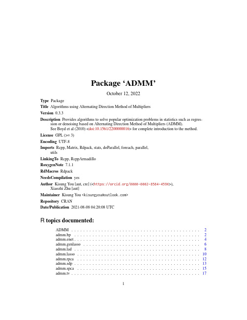
ADMM包：基于交替方向多项式方法的算法解决统计优化问题说明书

Package‘ADMM’October12,2022Type PackageTitle Algorithms using Alternating Direction Method of MultipliersVersion0.3.3Description Provides algorithms to solve popular optimization problems in statistics such as regres-sion or denoising based on Alternating Direction Method of Multipliers(ADMM).See Boyd et al(2010)<doi:10.1561/2200000016>for complete introduction to the method. License GPL(>=3)Encoding UTF-8Imports Rcpp,Matrix,Rdpack,stats,doParallel,foreach,parallel,utilsLinkingTo Rcpp,RcppArmadilloRoxygenNote7.1.1RdMacros RdpackNeedsCompilation yesAuthor Kisung You[aut,cre](<https:///0000-0002-8584-459X>),Xiaozhi Zhu[aut]Maintainer Kisung You<*********************>Repository CRANDate/Publication2021-08-0804:20:08UTCR topics documented:ADMM (2)admm.bp (2)admm.enet (4)admm.genlasso (6)d (8)sso (10)admm.rpca (12)admm.sdp (13)admm.spca (15) (17)1Index20 ADMM ADMM:Algorithms using Alternating Direction Method of Multipli-ersDescriptionAn introduction of Alternating Direction Method of Multipliers(ADMM)method has been a break-through in solving complex and non-convex optimization problems in a reasonably stable as well as scalable fashion.Our package aims at providing handy tools for fast computation on well-known problems using the method.For interested users/readers,please visit Prof.Stephen Boyd’s website entirely devoted to the topic.admm.bp Basis PursuitDescriptionFor an underdetermined system,Basis Pursuit aims toﬁnd a sparse solution that solvesmin x x 1s.t Ax=bwhich is a relaxed version of strict non-zero supportﬁnding problem.The implementation is bor-rowed from Stephen Boyd’s MATLAB code.Usageadmm.bp(A,b,xinit=NA,rho=1,alpha=1,abstol=1e-04,reltol=0.01,maxiter=1000)ArgumentsA an(m×n)regressor matrixb a length-m response vectorxinit a length-n vector for initial valuerho an augmented Lagrangian parameteralpha an overrelaxation parameter in[1,2]abstol absolute tolerance stopping criterionreltol relative tolerance stopping criterionmaxiter maximum number of iterationsValuea named list containingx a length-n solution vectorhistory dataframe recording iteration numerics.See the section for more details.Iteration HistoryWhen you run the algorithm,output returns not only the solution,but also the iteration history recording followingﬁelds over iterates,objval object(cost)function valuer_norm norm of primal residuals_norm norm of dual residualeps_pri feasibility tolerance for primal feasibility conditioneps_dual feasibility tolerance for dual feasibility conditionIn accordance with the paper,iteration stops when both r_norm and s_norm values become smaller than eps_pri and eps_dual,respectively.Examples##generate sample datan=30m=10A=matrix(rnorm(n*m),nrow=m)#design matrixx=c(stats::rnorm(3),rep(0,n-3))#coefficientx=base::sample(x)b=as.vector(A%*%x)#response##run exampleoutput=admm.bp(A,b)niter=length(output$history$s_norm)history=output$history##report convergence plotopar<-par(no.readonly=TRUE)par(mfrow=c(1,3))plot(1:niter,history$objval,"b",main="cost function")plot(1:niter,history$r_norm,"b",main="primal residual")plot(1:niter,history$s_norm,"b",main="dual residual")par(opar)admm.enet Elastic Net RegularizationDescriptionElastic Net regularization is a combination of 2stability and 1sparsity constraint simulatenously solving the following,min x 12Ax−b 22+λ1 x 1+λ2 x 22with nonnegative constraintsλ1andλ2.Note that if both lambda values are0,it reduces to least-squares solution.Usageadmm.enet(A,b,lambda1=1,lambda2=1,rho=1,abstol=1e-04,reltol=0.01,maxiter=1000)ArgumentsA an(m×n)regressor matrixb a length-m response vectorlambda1a regularization parameter for 1termlambda2a regularization parameter for 2termrho an augmented Lagrangian parameterabstol absolute tolerance stopping criterionreltol relative tolerance stopping criterionmaxiter maximum number of iterationsValuea named list containingx a length-n solution vectorhistory dataframe recording iteration numerics.See the section for more details.Iteration HistoryWhen you run the algorithm,output returns not only the solution,but also the iteration history recording followingﬁelds over iterates,objval object(cost)function valuer_norm norm of primal residuals_norm norm of dual residualeps_pri feasibility tolerance for primal feasibility conditioneps_dual feasibility tolerance for dual feasibility conditionIn accordance with the paper,iteration stops when both r_norm and s_norm values become smaller than eps_pri and eps_dual,respectively.Author(s)Xiaozhi ZhuReferencesZou H,Hastie T(2005).“Regularization and variable selection via the elastic net.”Journal of the Royal Statistical Society:Series B(Statistical Methodology),67(2),301–320.ISSN1369-7412, 1467-9868,doi:10.1111/j.14679868.2005.00503.x.See AlsossoExamples##generate underdetermined design matrixm=50n=100p=0.1#percentange of non-zero elementsx0=matrix(Matrix::rsparsematrix(n,1,p))A=matrix(rnorm(m*n),nrow=m)for(i in1:ncol(A)){A[,i]=A[,i]/sqrt(sum(A[,i]*A[,i]))}b=A%*%x0+sqrt(0.001)*matrix(rnorm(m))##run example with both regularization values=1output=admm.enet(A,b,lambda1=1,lambda2=1)niter=length(output$history$s_norm)history=output$history##report convergence plotopar<-par(no.readonly=TRUE)par(mfrow=c(1,3))plot(1:niter,history$objval,"b",main="cost function")plot(1:niter,history$r_norm,"b",main="primal residual") plot(1:niter,history$s_norm,"b",main="dual residual") par(opar)admm.genlasso Generalized LASSODescriptionGeneralized LASSO is solving the following equation,min x 12Ax−b 22+λ Dx 1where the choice of regularization matrix D leads to different problem formulations.Usageadmm.genlasso(A,b,D=diag(length(b)),lambda=1,rho=1,alpha=1,abstol=1e-04,reltol=0.01,maxiter=1000)ArgumentsA an(m×n)regressor matrixb a length-m response vectorD a regularization matrix of n columnslambda a regularization parameterrho an augmented Lagrangian parameteralpha an overrelaxation parameter in[1,2]abstol absolute tolerance stopping criterionreltol relative tolerance stopping criterionmaxiter maximum number of iterationsValuea named list containingx a length-n solution vectorhistory dataframe recording iteration numerics.See the section for more details.Iteration HistoryWhen you run the algorithm,output returns not only the solution,but also the iteration history recording followingﬁelds over iterates,objval object(cost)function valuer_norm norm of primal residuals_norm norm of dual residualeps_pri feasibility tolerance for primal feasibility conditioneps_dual feasibility tolerance for dual feasibility conditionIn accordance with the paper,iteration stops when both r_norm and s_norm values become smaller than eps_pri and eps_dual,respectively.Author(s)Xiaozhi ZhuReferencesTibshirani RJ,Taylor J(2011).“The solution path of the generalized lasso.”The Annals of Statistics, 39(3),1335–1371.ISSN0090-5364,doi:10.1214/11AOS878.Zhu Y(2017).“An Augmented ADMM Algorithm With Application to the Generalized Lasso Problem.”Journal of Computational and Graphical Statistics,26(1),195–204.ISSN1061-8600, 1537-2715,doi:10.1080/10618600.2015.1114491.Examples##generate sample datam=100n=200p=0.1#percentange of non-zero elementsx0=matrix(Matrix::rsparsematrix(n,1,p))A=matrix(rnorm(m*n),nrow=m)for(i in1:ncol(A)){A[,i]=A[,i]/sqrt(sum(A[,i]*A[,i]))}b=A%*%x0+sqrt(0.001)*matrix(rnorm(m))D=diag(n);##set regularization lambda valueregval=0.1*Matrix::norm(t(A)%*%b, I )##solve LASSO via reducing from Generalized LASSOoutput=admm.genlasso(A,b,D,lambda=regval)#set D as identity matrixniter=length(output$history$s_norm)history=output$history##report convergence plotopar<-par(no.readonly=TRUE)par(mfrow=c(1,3))plot(1:niter,history$objval,"b",main="cost function")plot(1:niter,history$r_norm,"b",main="primal residual")plot(1:niter,history$s_norm,"b",main="dual residual")par(opar)d Least Absolute DeviationsDescriptionLeast Absolute Deviations(LAD)is an alternative to traditional Least Sqaures by using cost func-tionmin x Ax−b 1to use 1norm instead of square loss for robust estimation of coefﬁcient.Usaged(A,b,xinit=NA,rho=1,alpha=1,abstol=1e-04,reltol=0.01,maxiter=1000)ArgumentsA an(m×n)regressor matrixb a length-m response vectorxinit a length-n vector for initial valuerho an augmented Lagrangian parameteralpha an overrelaxation parameter in[1,2]abstol absolute tolerance stopping criterionreltol relative tolerance stopping criterionmaxiter maximum number of iterationsValuea named list containingx a length-n solution vectorhistory dataframe recording iteration numerics.See the section for more details.Iteration HistoryWhen you run the algorithm,output returns not only the solution,but also the iteration history recording followingﬁelds over iterates,objval object(cost)function valuer_norm norm of primal residuals_norm norm of dual residualeps_pri feasibility tolerance for primal feasibility conditioneps_dual feasibility tolerance for dual feasibility conditionIn accordance with the paper,iteration stops when both r_norm and s_norm values become smaller than eps_pri and eps_dual,respectively.Examples##generate datam=1000n=100A=matrix(rnorm(m*n),nrow=m)x=10*matrix(rnorm(n))b=A%*%x##add impulsive noise to10%of positionsidx=sample(1:m,round(m/10))b[idx]=b[idx]+100*rnorm(length(idx))##run the codeoutput=d(A,b)niter=length(output$history$s_norm)history=output$history##report convergence plotopar<-par(no.readonly=TRUE)par(mfrow=c(1,3))plot(1:niter,history$objval,"b",main="cost function")plot(1:niter,history$r_norm,"b",main="primal residual")plot(1:niter,history$s_norm,"b",main="dual residual")par(opar)sso sso Least Absolute Shrinkage and Selection OperatorDescriptionLASSO,or L1-regularized regression,is an optimization problem to solvemin x 12Ax−b 22+λ x 1for sparsifying the coefﬁcient vector x.The implementation is borrowed from Stephen Boyd’s MATLAB code.Usagesso(A,b,lambda=1,rho=1,alpha=1,abstol=1e-04,reltol=0.01,maxiter=1000)ArgumentsA an(m×n)regressor matrixb a length-m response vectorlambda a regularization parameterrho an augmented Lagrangian parameteralpha an overrelaxation parameter in[1,2]abstol absolute tolerance stopping criterionreltol relative tolerance stopping criterionmaxiter maximum number of iterationsValuea named list containingx a length-n solution vectorhistory dataframe recording iteration numerics.See the section for more details.sso11Iteration HistoryWhen you run the algorithm,output returns not only the solution,but also the iteration history recording followingﬁelds over iterates,objval object(cost)function valuer_norm norm of primal residuals_norm norm of dual residualeps_pri feasibility tolerance for primal feasibility conditioneps_dual feasibility tolerance for dual feasibility conditionIn accordance with the paper,iteration stops when both r_norm and s_norm values become smaller than eps_pri and eps_dual,respectively.ReferencesTibshirani R(1996).“Regression Shrinkage and Selection via the Lasso.”Journal of the Royal Statistical Society.Series B(Methodological),58(1),267–288.ISSN00359246.Examples##generate sample datam=50n=100p=0.1#percentange of non-zero elementsx0=matrix(Matrix::rsparsematrix(n,1,p))A=matrix(rnorm(m*n),nrow=m)for(i in1:ncol(A)){A[,i]=A[,i]/sqrt(sum(A[,i]*A[,i]))}b=A%*%x0+sqrt(0.001)*matrix(rnorm(m))##set regularization lambda valuelambda=0.1*base::norm(t(A)%*%b,"F")##run exampleoutput=sso(A,b,lambda)niter=length(output$history$s_norm)history=output$history##report convergence plotopar<-par(no.readonly=TRUE)par(mfrow=c(1,3))plot(1:niter,history$objval,"b",main="cost function")plot(1:niter,history$r_norm,"b",main="primal residual")plot(1:niter,history$s_norm,"b",main="dual residual")par(opar)12admm.rpca admm.rpca Robust Principal Component AnalysisDescriptionGiven a data matrix M,itﬁnds a decompositionmin L ∗+λ S 1s.t.L+S=Mwhere L ∗represents a nuclear norm for a matrix L and S 1=|S i,j|,andλa balanc-ing/regularization parameter.The choice of such norms leads to impose low-rank property for L and sparsity on S.Usageadmm.rpca(M,lambda=1/sqrt(max(nrow(M),ncol(M))),mu=1,tol=1e-07,maxiter=1000)ArgumentsM an(m×n)data matrixlambda a regularization parametermu an augmented Lagrangian parametertol relative tolerance stopping criterionmaxiter maximum number of iterationsValuea named list containingL an(m×n)low-rank matrixS an(m×n)sparse matrixhistory dataframe recording iteration numerics.See the section for more details.Iteration HistoryFor RPCA implementation,we chose a very simple stopping criterionM−(L k+S k) F≤tol∗ M Ffor each iteration step k.So for this method,we provide a vector of only relative errors,error relative error computedReferencesCandès EJ,Li X,Ma Y,Wright J(2011).“Robust principal component analysis?”Journal of the ACM,58(3),1–37.ISSN00045411,doi:10.1145/1970392.1970395.Examples##generate data matrix from standard normalX=matrix(rnorm(20*5),nrow=5)##try different regularization valuesout1=admm.rpca(X,lambda=0.01)out2=admm.rpca(X,lambda=0.1)out3=admm.rpca(X,lambda=1)##visualize sparsityopar<-par(no.readonly=TRUE)par(mfrow=c(1,3))image(out1$S,main="lambda=0.01")image(out2$S,main="lambda=0.1")image(out3$S,main="lambda=1")par(opar)admm.sdp Semideﬁnite ProgrammingDescriptionWe solve the following standard semideﬁnite programming(SDP)problemmin X tr(CX)s.t.A(X)=b,X≥0with A(X)i=tr(A i X)=b i for i=1,...,m and X≥0stands for positive-deﬁniteness of the matrix X.In the standard form,matrices C,A1,A2,...,A m are symmetric and solution X would be symmetric and positive semideﬁnite.This function implements alternating direction augmented Lagrangian methods.Usageadmm.sdp(C,A,b,mu=1,rho=1,abstol=1e-10,maxiter=496,print.progress=FALSE)ArgumentsC an(n×n)symmetric matrix for cost.A a length-m list of(n×n)symmetric matrices for constraint.b a length-m vector for equality condition.mu penalty parameter;positive real number.rho step size for updating in(0,1+√5).2abstol absolute tolerance stopping criterion.maxiter maximum number of iterations.print.progress a logical;TRUE to show the progress,FALSE to go silent.Valuea named list containingx a length-n solution vectorhistory dataframe recording iteration numerics.See the section for more details.Iteration HistoryWhen you run the algorithm,output returns not only the solution,but also the iteration history recording followingﬁelds over iterates,objval object(cost)function valueeps_pri feasibility tolerance for primal feasibility conditioneps_dual feasibility tolerance for dual feasibility conditiongap gap between primal and dual cost function.We use the stopping criterion which breaks the iteration when all eps_pri,eps_dual,and gap become smaller than abstol.Author(s)Kisung YouReferencesWen Z,Goldfarb D,Yin W(2010).“Alternating direction augmented Lagrangian methods for semideﬁnite programming.”Mathematical Programming Computation,2(3-4),203–230.ISSN 1867-2949,1867-2957,doi:10.1007/s1253201000171.Examples##a toy example#generate parametersC=matrix(c(1,2,3,2,9,0,3,0,7),nrow=3,byrow=TRUE)A1=matrix(c(1,0,1,0,3,7,1,7,5),nrow=3,byrow=TRUE)A2=matrix(c(0,2,8,2,6,0,8,0,4),nrow=3,byrow=TRUE)A=list(A1,A2)b=c(11,19)#run the algorithmrun=admm.sdp(C,A,b)hst=run$history#visualizeopar<-par(no.readonly=TRUE)par(mfrow=c(2,2))plot(hst$objval,type="b",cex=0.25,main="objective value")plot(hst$eps_pri,type="b",cex=0.25,main="primal feasibility") plot(hst$eps_dual,type="b",cex=0.25,main="dual feasibility") plot(hst$gap,type="b",cex=0.25,main="primal-dual gap")par(opar)##Not run:##comparison with CVXR s resultrequire(CVXR)#problems definitionX=Variable(3,3,PSD=TRUE)myobj=Minimize(sum_entries(C*X))#objectivemycon=list(#constraintsum_entries(A[[1]]*X)==b[1],sum_entries(A[[2]]*X)==b[2])myp=Problem(myobj,mycon)#problem#run and visualizeres=solve(myp)Xsol=res$getValue(X)opar=par(no.readonly=TRUE)par(mfrow=c(1,2),pty="s")image(run$X,axes=FALSE,main="ADMM result")image(Xsol,axes=FALSE,main="CVXR result")par(opar)##End(Not run)admm.spca Sparse PCADescriptionSparse Principal Component Analysis aims atﬁnding a sparse vector by solvingmax x x TΣx s.t. x 2≤1, x 0≤Kwhere x 0is the number of non-zero elements in a vector x.A convex relaxation of this problem was proposed to solve the following problem,max X<Σ,X>s.t.T r(X)=1, X 0≤K2,X≥0,rank(X)=1 where X=xx T is a(p×p)matrix that is outer product of a vector x by itself,and X≥0means the matrix X is positive semideﬁnite.With the rank condition dropped,it can be restated asmax X<Σ,X>−ρ X 1s.t.T r(X)=1,X≥0.After acquiring each principal component vector,an iterative step based on Schur complement deﬂation method is applied to regress out the impact of previously-computed projection vectors.It should be noted that those sparse basis may not be orthonormal.Usageadmm.spca(Sigma,numpc,mu=1,rho=1,abstol=1e-04,reltol=0.01,maxiter=1000)ArgumentsSigma a(p×p)(sample)covariance matrix.numpc number of principal components to be extracted.mu an augmented Lagrangian parameter.rho a regularization parameter for sparsity.abstol absolute tolerance stopping criterion.reltol relative tolerance stopping criterion.maxiter maximum number of iterations.Valuea named list containingbasis a(p×numpc)matrix whose columns are sparse principal components.history a length-numpc list of dataframes recording iteration numerics.See the section for more details.Iteration HistoryFor SPCA implementation,main computation is sequentially performed for each projection vector.The historyﬁeld is a list of length numpc,where each element is a data frame containing iteration history recording followingﬁelds over iterates,r_norm norm of primal residuals_norm norm of dual residualeps_pri feasibility tolerance for primal feasibility conditioneps_dual feasibility tolerance for dual feasibility conditionIn accordance with the paper,iteration stops when both r_norm and s_norm values become smaller than eps_pri and eps_dual,respectively.ReferencesMa S(2013).“Alternating Direction Method of Multipliers for Sparse Principal Component Anal-ysis.”Journal of the Operations Research Society of China,1(2),253–274.ISSN2194-668X, 2194-6698,doi:10.1007/s4030501300169.Examples##generate a random matrix and compute its sample covarianceX=matrix(rnorm(1000*5),nrow=1000)covX=stats::cov(X)##compute3sparse basisoutput=admm.spca(covX,3) Total Variation MinimizationDescription1-dimensional total variation minimization-also known as signal denoising-is to solve the follow-ingmin x 12x−b 22+λi|x i+1−x i|for a given signal b.The implementation is borrowed from Stephen Boyd’s MATLAB code.Usage(b,lambda=1,xinit=NA,rho=1,alpha=1,abstol=1e-04,reltol=0.01,maxiter=1000)Argumentsb a length-m response vectorlambda regularization parameterxinit a length-m vector for initial valuerho an augmented Lagrangian parameteralpha an overrelaxation parameter in[1,2]abstol absolute tolerance stopping criterionreltol relative tolerance stopping criterionmaxiter maximum number of iterationsValuea named list containingx a length-m solution vectorhistory dataframe recording iteration numerics.See the section for more details.Iteration HistoryWhen you run the algorithm,output returns not only the solution,but also the iteration history recording followingﬁelds over iterates,objval object(cost)function valuer_norm norm of primal residuals_norm norm of dual residualeps_pri feasibility tolerance for primal feasibility conditioneps_dual feasibility tolerance for dual feasibility conditionIn accordance with the paper,iteration stops when both r_norm and s_norm values become smaller than eps_pri and eps_dual,respectively.Examples##generate sample datax1=as.vector(sin(1:100)+0.1*rnorm(100))x2=as.vector(cos(1:100)+0.1*rnorm(100)+5)x3=as.vector(sin(1:100)+0.1*rnorm(100)+2.5)xsignal=c(x1,x2,x3)##run exampleoutput=(xsignal)##visualizeopar<-par(no.readonly=TRUE)plot(1:300,xsignal,type="l",main="TV Regularization") lines(1:300,output$x,col="red",lwd=2)par(opar)IndexADMM,2ADMM-package(ADMM),2admm.bp,2admm.enet,4admm.genlasso,6d,8sso,5,10admm.rpca,12admm.sdp,13admm.spca,15,1720。

二阶锥互补问题求解方法研究

二阶锥互补问题求解方法研究The second-order cone complementarity problem (SOCCP) is a class of nonlinear optimization problems that arise in various fields such as operations research, economics, and engineering. It involves finding a point in a specific cone that satisfies a set of complementarity conditions. 二阶锥互补问题是一类在运筹学、经济学和工程学等领域中出现的非线性优化问题。

它涉及找到在特定锥体中满足一组互补条件的点。

One method for solving SOCCP is the interior-point method, which relies on the concept of central path. This method involves solving a sequence of primal-dual equations that approach the central path, eventually reaching the solution to the SOCCP. 一种解决二阶锥互补问题的方法是内点法，该方法依赖于中心路径的概念。

这种方法涉及解决一系列逼近中心路径的原始-对偶方程，最终达到二阶锥互补问题的解。

Another approach is the splitting method, which involves breaking down the problem into smaller subproblems and solving them iteratively. This method can be effective for large-scale problems by reducing the computational complexity. 拆分方法是另一种方法，它涉及将问题分解成较小的子问题，并通过迭代解决它们。

内点法介绍(Interior Point Method)

内点法介绍（Interior Point Method）在面对无约束的优化命题时，我们可以采用牛顿法等方法来求解。

而面对有约束的命题时，我们往往需要更高级的算法。

单纯形法（Simplex Method）可以用来求解带约束的线性规划命题（LP），与之类似的有效集法（Active Set Method）可以用来求解带约束的二次规划（QP），而内点法（Interior Point Method）则是另一种用于求解带约束的优化命题的方法。

而且无论是面对LP还是QP，内点法都显示出了相当的极好的性能，例如多项式的算法复杂度。

本文主要介绍两种内点法，障碍函数法（Barrier Method）和原始对偶法（Primal-Dual Method）。

其中障碍函数法的内容主要来源于Stephen Boyd与Lieven Vandenberghe的Convex Optimization一书，原始对偶法的内容主要来源于Jorge Nocedal和Stephen J. Wright的Numerical Optimization一书（第二版）。

为了便于与原书对照理解，后面的命题与公式分别采用了对应书中的记法，并且两者方法针对的是不同的命题。

两种方法中的同一变量可能在不同的方法中有不同的意义，如μ。

在介绍玩两种方法后会有一些比较。

障碍函数法Barrier MethodCentral Path举例原始对偶内点法Primal Dual Interior Point Method Central Path举例几个问题障碍函数法（Barrier Method）对于障碍函数法，我们考虑一个一般性的优化命题：minsubject tof0(x)fi(x)≤0,i=1,...,mAx=b(1) 这里f0,...,fm:Rn→R 是二阶可导的凸函数。

同时我也要求命题是有解的，即最优解x 存在，且其对应的目标函数为p。

此外，我们还假设原命题是可行的（feasible）。

基于SOP和VSC的交直流混合配电网多时间尺度优化控制

基于SOP和VSC的交直流混合配电网多时间尺度优化控制张博;唐巍;丛鹏伟;张筱慧;娄铖伟【摘要】智能软开关(SOP)、电压源换流器(VSC)等电力电子设备具备快速灵活的功率调节能力,能够有效应对分布式电源带来的随机性和波动性.本文分析了含SOP 和VSC的交直流混合配电网基本结构,针对高渗透率分布式电源接入带来的高损耗和电压越限问题,提出了一种多时间尺度协调控制方法.在日前时间尺度上,针对离散的开关变量与连续的SOP、VSC功率,以降低损耗为优化目标建立分层协调调度模型;在日内短时时间尺度上,针对电压越限风险情况,以控制电压为优化目标快速调整SOP、VSC功率.采用基于蚁群算法和原对偶内点法的混合优化算法对所提出的模型进行求解,实现联络开关与SOP、VSC功率的联立优化.通过算例仿真验证了所提模型和算法的有效性.%Power electronic equipment such as soft open point ( SOP) and voltage source converter ( VSC) can ef-fectively cope with the randomness and fluctuation of distributed generation ( DG) with fast and flexible ability of power regulation. Structure of hybrid AC/DC distribution networks with SOP and VSC is analyzed. A multi-time scale coordinated control method is proposed, which aims at high power losses and out-of-limit voltage caused by in-tegration of large number of DG. Taking switch states and power of VSC and SOP as optimization variables, a hier-archical coordination model with the objective of minimized network loss is established at day-ahead time scales. In the short time scale, voltage deviations are minimized in the risk state by regulating power of SOP and VSC. A hy-brid optimization algorithm based on ant colony algorithm and primal-dual interior point method is proposed to solve the problem andrealize coordinated optimization of switch states and power of VSC and SOP. The efficiency of the proposed model and method are verified in a case study.【期刊名称】《电工电能新技术》【年(卷),期】2017(036)009【总页数】9页(P11-19)【关键词】交直流混合配电网;智能软开关;电压源换流器;多时间尺度【作者】张博;唐巍;丛鹏伟;张筱慧;娄铖伟【作者单位】中国农业大学信息与电气工程学院,北京100083;中国农业大学信息与电气工程学院,北京100083;中国农业大学信息与电气工程学院,北京100083;中国农业大学信息与电气工程学院,北京100083;中国农业大学信息与电气工程学院,北京100083【正文语种】中文【中图分类】TM73随着配电网规模的不断扩大以及风力、光伏等大量可再生能源的接入，未来配电网的结构以及运行方式将更加复杂。

一种求解正交约束问题的投影梯度方法

一种求解正交约束问题的投影梯度方法童谣;丁卫平【摘要】The orthogonality constrained problems has wide applications in eigenvalue problems, sparse principal component analysis, etc. However, it is challenging to solve orthogonality constrained problems due to the non-convexity of the equality constraint. This paper proposes a projection gradient method using Gram-Schmidt process to deal with the orthogonality constraint. The time complexity is bounded by O ( r2 n), which is lower than the classical SVD. Some primary numerical results verified the validity of the proposed method.%摘正交约束优化问题在特征值问题、稀疏主成分分析等方面有广泛的应用。

由于正交约束的非凸性，精确求解该类问题具有一定的困难。

本文提出了一种求解正交约束优化问题的投影梯度算法。

该算法采用施密特标准正交化方法处理正交约束，其时间复杂度为 O ( r2 n)，比传统 SVD 分解复杂度低，且实现简单。

数值实验验证了算法的有效性。

【期刊名称】《湖南理工学院学报（自然科学版）》【年(卷),期】2015(000)002【总页数】5页(P5-9)【关键词】正交约束优化;投影梯度算法;邻近点算法;施密特标准正交化【作者】童谣;丁卫平【作者单位】福州大学数学与计算机科学学院，福州 350108;湖南理工学院数学学院，湖南岳阳 414006【正文语种】中文【中图分类】O224正交约束优化模型在科学与工程计算相关领域有广泛应用, 譬如: 线性和非线性特征值问题[1,2], 组合优化问题[3,4], 稀疏主成分分析问题[5,6], 人脸识别[7], 基因表达数据分析[8], 保角几何[10,11], 1-比特压缩传感[12～14], p-调和流[15～18], 等等, 都离不开正交约束优化模型.一般地, 正交约束优化问题有如下形式:其中F( X)是ℝn×r→ℝ的可微函数, Q是对称正定阵, I是r×r单位阵, n≥r. 由于Q是对称正定的, 可设Q=LT L. 令Y=LX, 则(1)可转化为:线性约束优化问题的求解技术已经比较成熟, 为了简化问题(2)的形式, 我们主要考虑求解如下正交约束优化问题:由于正交约束的非凸性, 精确求解问题(1)或(3)具有一定的挑战. 目前为止, 还没有有效的算法可以保证获取这类问题的全局最优解(除了某些特殊情况, 如: 寻找极端特征值). 由于保持正交约束可行性的计算代价太大, 为了避免直接处理非线性约束, 人们提出了很多方法, 将带约束的优化问题转化成无约束的优化问题求解. 这些方法中, 最常用的有罚函数方法[21,22]和增广拉格朗日方法[19,20].罚函数方法将正交约束违背作为惩罚项添加到目标函数中, 把约束优化问题(3)转化为如下无约束优化问题:其中ρ＞0为罚参数. 当罚参数趋于无穷大时, 罚问题(4)与原问题(3)等价. 为了克服这个缺陷, 人们引入了标准增广拉格朗日方法. Wen和Yang等[23]提出用Lagrange方法求解问题并证明了算法收敛于问题的可行解(在正则条件下, 收敛到平衡点). 最近, Manton [24,25] 等提出了解决正交约束问题的Stiefel manifold 结构方法: Osher [26] 等提出一种基于Bregman迭代的SOC算法. SOC算法结合算子分裂与Bregman迭代方法, 将正交约束问题转化为交替求解一个无约束优化问题和一个具有解析解的二次约束优化问题, 该方法获得了不错的数值实验效果. SOC算法在处理矩阵正交约束的子问题时,使用了传统的SVD分解, 其时间复杂度为O( n3).在本文中, 我们提出一种新的处理正交约束的算法, 该算法计算复杂性比传统的SVD分解要低. 根据问题(3)约束条件的特殊性, 我们将问题求解过程分解为两步: 第一步, 采用邻近点算法求解松弛的无约束优化问题, 得到预测点; 第二步, 将预测点投影到正交约束闭子集上. 基本的数值结果说明了这种正交闭子集投影梯度算法优越于经典增广Lagrange算法.本节给出求解正交约束优化问题的正交闭子集上的投影梯度算法(简记为POPGM). 该方法分为两步: 首先, 采用邻近点算法求解松弛的无约束优化问题, 得到预测点; 然后, 将预测点投影到正交闭子集上, 其中投影算子是一个简单的斯密特标准正交化过程. 为此, 我们先简要介绍邻近点算法.1.1 经典邻近点算法求解无约束优化问题的方法有很多, 包括: 最速下降法, Barzilai-Borwein method[30], 外梯度方法[31],等等. 这里, 我们介绍一种有效的求解算法, 邻近点算法(Proximal Point Algorithm, 简记为PPA)[27,28]. 最初, Rockafellar等[32]提出了求解变分不等式问题的PPA算法. 对于抽象约束优化问题:1.2 投影梯度算法现在给出本文提出的邻近点正交约束投影梯度算法(POPGM):Step 0. 给定初始参数r0＞0, v=0.95, 初始点X0∈Ω, 给定ε＞0, ρ＞1, 令k=0. 注: 子问题(10)等价于求解如下单调变分不等式变分不等式(12)可采用下述显示投影来获得逼近解:由于(11)和(13)均有显示表达式, 可知和Xk都是易于求解的. 另外, 由于r<<n, 与传统SVD分解方法的时间复杂度O( n3)相比, 本文所提出的在正交约束闭子集上投影梯度法的计算时间花费更少, 这是因为(11)式处理正交约束的时间复杂度仅需O( r2 n).本节通过实例来说明POPGM算法的有效性. 实验测试环境为Win7系统,Intel(R)Core i3, CPU .20GHz, RAM 2.0GB, 编程软件为MATLAB R2012b.测试问题及数据取自Yin0. 给定对称矩阵A∈ℝn×n , 和酉矩阵V∈ℝn×r , 当V 是前r个最大特征值所对应特征空间的一组正交基时, 函数Trace(VT AV)达到最大值. 该问题可以考虑为求解如下正交约束优化问题:其中λ1≥λ2≥…≥λr 是我们要提取A的r个最大的特征值, A∈ℝn×n 为对称正定矩阵.实验数据:, 其中, 即中的元素服从均匀分布.实验参数:,ρ=1.6, ε=1.0e-5.初始点: X0=randn(n, r), X0=orth(X0).终止条件: .下面采用三种算法求解上述问题, 分别是本文的POPGM算法, Yin0的algorithm 2(简记为Yin’s Algo.)与MATLAB工具包中的“eigs”函数. 表中的FP/FY/FE 分别表示通过运行POPGM、Yin’s Algo和Eigs所求得的r个最大特征值之和, 即目标函数值; win表示两种算法对比, 所获得的目标函数值之差; err表示可行性误差, 即: e.表1给出了对于固定r=6, n 在500到5000之间变化时, 三种算法在求解问题的迭代次数(iter)与CPU时间(cput)的对比结果. 由表1可知, POPGM迭代次数受矩阵维数影响不大. 随着矩阵维数的增大, POPGM算法与Yin’s Algo.相比, 当n≤2000时, POPGM不仅时间上有优势, 而且提取效果也较好(win＞0); n≥3000时, POPGM时间花费略多, 但提取效果有明显优势. POPGM与“eigs”相比, 随着维数n的增大, 时间优势逐渐变大, 但提取变量的解释能力也逐渐减弱. 由实验结果可知, 当矩阵维数n较大时, POPGM有较好的表现.表2列出了固定n=3000, 提取特征值的个数r在1到23之间变化时POPGM的运行结果. 由表2可以看出, 当r越小, POPGM计算花费时间越少; 随着r增大, FP 增大, 时间花费也在增大; 当r取5到7时, 花费时间合适, 且提取效果较好.表3列出了固定提取r=6, 将POPGM算法框架中的正交化过程替换成SVD分解, 对比两种处理正交约束方法的求解结果. 由表3可知, 在POPGM算法框架下, 在正交约束闭子集上的投影算子比传统的SVD分解在运算时间上要节约很多; 同时, 两种方法所提取的特征之和保持一致, 不随维数变化而变化,时间优势随矩阵维数增大而增大. 可见, 本文提出的处理正交约束的方法非常有效.本文研究求解一类正交约束优化问题的快速算法. 结合邻近点算法和施密特标准正交化过程, 本文提出了基于邻近点算法的非精确投影梯度算法, 算法采用邻近点算法求解松弛的无约束优化问题, 得到预测点; 然后, 将预测点投影到正交约束闭子集上. 与传统的增广拉格朗日法、罚函数方法的主要区别在于POPGM在每一步迭代中通过在正交约束集上投影得到迭代解, 并且避免使用SVD分解, 加快了算法的运行速度. 数值实验说明本文提出的POPGM有较好的综合表现.【相关文献】[1] Edelman A., As T., Arias A., Smith T., et al. The geometry of algorithms with orthogonality constraints [J]. SIAM J. Matrix Anal. Appl., 1998, 20 (2): 303～353[2] Caboussat A., Glowinski R., Pons V. An augmented lagrangian approach to the numerical solution of a non-smooth eigenvalue problem [J]. J. Numer. Math., 2009, 17 (1): 3～26[3] Burkard R. E., Karisch S. E., Rendl F. Qaplib-a quadratic assignment problem library [J]. J. Glob. Optim., 1997, 10 (4): 291～403[4] Loiola E. M., de Arbreu N. M. M., Boaventura –Netto P. O., et al. A survey for thequadratic assignment problem[J]. Eur. J. Oper. Res., 2007, 176 (2): 657～690[5] Lu Z. S., Zhang Y. An augmented lagrangian approach for sparse principal component analysis[J]. Math. Program., Ser. A., 2012, 135: 149～193[6] Shen H., Huang J. Z. Sparse principal component analysis via regularized low rank matrix approximation[J]. J. Multivar. Anal., 2008, 99 (6): 1015～1034[7] Hancock P. Burton A., Bruce V. Face processing: human perception and principal components analysis[J]. Memory Cogn., 1996, 24: 26～40[8] Botstein D. Gene shavingas a method for identifying distinct sets of genes with similar expression patterns[J]. Genme Bil., 2000, 1: 1～21[9] Wen Z., Yin W. T. A feasible method for optimization with orthogonality constraints[J]. Math. Program., 2013, 143(1-2): 397～434[10] Gu X., Yau S. Computing conformal structures of surfaces[J]. Commun. Inf. Syst., 2002, 2 (2): 121～146[11] Gu X., Yau S. T. Global conformal surface parameterization[C]. In Symposium on Geometry Processing, 2003: 127～137[12] Boufounos P. T., Baraniuk R. G. 1-bit compressive sensing [C]. In Conference on information Sciences and Systems (CISS), IEEE, 2008: 16～21[13] Yan M., Yang Y., Osher S. Robust 1-bit compressive sensing using adaptive outlier pursuit [J]. IEEE Trans, Signal Process, 2012, 60 (7): 3868～3875[14] Laska J. N., Wen Z., Yin W., Baraniuk R. G. Trust, but verify: fast and accurate signal recovery from 1-bit compressive measurements [J]. IEEE Trans. Signal Process, 2011, 59 (11): 5289[15] Chan T. F., Shen J. Variational restoration of nonflat image features: models and algorithms [J]. SIAM J. Appl. Math., 2000, 61: 1338～1361[16] Tang B., Sapiro G., Caselles V. Diffusion of general data on non-flat manifolds via harmonic maps theory: the direction diffusion case [J]. Int. J. Comput. Vis., 2000, 36: 149～161[17] Vese L. A., Osher S. Numerical method for p-harmonic flows and applications to image processing[J]. SIAM J. Numer. Anal., 2002, 40 (6): 2085～2104[18] Goldfarb D., Wen Z., Yin W. A curvilinear search method for the p-harmonic flow on spheres [J]. SIAM J. Imaging Sci., 2009, 2: 84～109[19] Glowinski R., Le Tallec P. Augmented Lagrangian and operator splitting methods in nonlinear mechanics [J]. SIAM Studies in Applied Mathematics, Society for Industrial and Applied Mathematics(SIAM), Philadelphia, PA, 1989, 9[20] Fortin M., Glowinski R. Augmented Lagrangian methods: applications to the numerical solution of boundary-value problems [J]. North Holland, 2000, 15[21] Nocedal J., Wright S. J. Numerical Optimization[M]. Springer, New York, 2006[22] Brthuel F., Brezis H., Helein F. Asymptotics for the minimization of a ginzburg-landau functional [J]. Calc. Var. Partial. Differ. Equ., 1993, 1 (2): 123～148[23] Wen Z., Yang C., Liu X. Trace-penalty minimization for large-scale eigenspace computation [J]. J. Scientific Comput., to appear[24] Manton J. H. Optimization algorithms exploiting unitary constraints [J]. IEEE Trans. Signal Process, 2002, 50 (3): 635～650[25] Absil P. -A., Mahony R., Sepulchre R. Optimization algorithms on matrix manifolds [M]. Princeton University Press, Princeton, 2008[26] Lai R., Osher S. A splitting method for orthogonality constrained problem [J]. J Sci Comput., 2014, 58 (2): 431～449[27] He B. S., Fu X. L. and Jiang Z. K. Proximal point algorithm using a linear proximal term [J]. J. Optim. Theory Appl., 2009, 141: 209～239[28] He B. S., Yuan X. M. Convergence analysis of primal-dual algorithms for a saddle-point problem: From contraction perspective [J]. SIAM J. Imaging Sci., 2012, 5: 1119～149 [29] Barzilai J., Borwein J. M. Two-point step size gradient methods [J]. IMA J. Numer. Anal., 1988, 8: 141～148[30] Korpelevich G. M. The extragradient method for finding saddle points and other problems [J]. Ekonomika Matematicheskie Metody, 1976, 12: 747～756[31] Rockafellar R. T. Monotone operators and the proximal point algorithms [J]. SIAM J. Cont. Optim., 1976, 14: 877～898。

相关主题

富士康科技集团简介

1、下载文档前请自行甄别文档内容的完整性，平台不提供额外的编辑、内容补充、找答案等附加服务。
2、"仅部分预览"的文档,不可在线预览部分如存在完整性等问题,可反馈申请退款(可完整预览的文档不适用该条件!)。
3、如文档侵犯您的权益，请联系客服反馈,我们会尽快为您处理(人工客服工作时间：9:00-18:30)。

QOS MULTIMEDIA MULTICAST ROUTINGA COMPONENT BASED PRIMAL DUAL APPROACHbyFAHEEM A HUSSAINUnder the Direction of Professor Alexander ZelikovskyABSTRACTThe QoS Steiner Tree Problem asks for the most cost eﬃcient way to multicast multimedia to a heterogeneous collection of users with diﬀerent data consumption rates.We assume that the cost of using a link is not constant but rather depends on the maximum bandwidth routed through the link.Formally,given a graph with costs on the edges,a source node and a set of terminal nodes,each one with a bandwidth requirement,the goal is toﬁnd a Steiner tree containing the source,and the cheapest assignment of bandwidth to each of its edges so that each source-to-terminal path in the tree has bandwidth at least as large as the bandwidth required by the terminal. Our main contributions are:(1)Newﬂow-based integer linear program formulation for the problem;(2)First implementation of4.311primal-dual constant factor ap-proximation algorithm;(3)an extensive experimental study of the new heuristics and of several previously proposed algorithms.INDEX WORDS:QOS,Multimedia multicast,Steiner tree,QOSST,4.311Primal dual,Maxemchuck,Naive PD,Restarting PD,Flow ILP,MST,Rate,BandwidthQOS MULTIMEDIA MULTICAST ROUTINGA COMPONENT BASED PRIMAL DUAL APPROACHbyFAHEEM A HUSSAINThesis Submitted in Partial Fulﬁllment of the Requirements for the Degree ofMaster of Sciencein the College of Arts and SciencesGeorgia State University2006c Copyright by Faheem A Hussain2006All Rights ReservedQOS MULTIMEDIA MULTICAST ROUTINGA COMPONENT BASED PRIMAL DUAL APPROACHbyFAHEEM A HUSSAINMajor Professor: Alexander ZelikovskyCommittee: Anu BourgeoisSaeid Belkasim Electronic Version Approved:Office of Graduate StudiesCollege of Arts and SciencesGeorgia State UniversityDecember 2006To my mother.ACKNOWLEDGMENTSThanks to my advisor Dr.Alex Zelikovsky for his tireless eﬀorts and help to make this happen.I also would like to thank the other committee members,Dr.Anu Bourgeois and Dr.Saeid Belkasim for their invaluable time spent in reviewing my thesis.In addition,I would like to thank my colleagues Kelly Westbrooks,Dumitru Brinza and Gulsah Altun for their help in accomplishing my thesis.TABLE OF CONTENTSPage ACKNOWLEDGMENTS (v)LIST OF TABLES (ix)LIST OF FIGURES (x)CHAPTER1.INTRODUCTION (1)1.1Motivation (1)1.2Problem Formulation (2)1.3Previous Work (3)1.4Contributions and Organization (4)2.HEURISTICS (5)2.1Maxemchuk’s Approach (5)2.2Naive Primal-Dual Method (6)2.3Restarting Primal-Dual Algorithm (7)2.4 4.311approximation Primal-Dual algorithm (8)2.4.1Algorithm Explanation (12)3.AN EXACT INTEGER LINEAR PROGRAM SOLUTION (16)3.1What is Linear Programming? (16)3.1.1Application areas (17)3.1.2Standard form (17)3.1.3Integer Linear Programs and Their Relaxations (18)3.2ILP Formulation for QOSST problem (19)3.2.1Variables (19)3.2.2Objective Function (20)3.2.3Flow Constraints (20)3.2.4Example (21)3.2.4.1ILP representation of QOSST in CPLEX (22)3.2.4.2ILP representation of QOSST in MathProg (23)3.2.4.3Output of GLPK (25)4.SOFTW ARE PACKAGE (29)4.1Planar Graph Generation (29)4.2Graphical User Interface (30)5.IMPLEMENTATION (31)5.1Speciﬁcations (31)5.2Design (33)5.2.1Package Diagram (33)5.2.1.1GLPK (34)5.2.1.2JGraphT (34)5.2.1.3JGraph (34)5.2.1.4SimQ (35)5.2.2Classes (35)5.2.2.1ColoredComboBoxRenderer (35)5.2.2.2ColoredRate (35)5.2.2.3CompoundVertexView (35)5.2.2.4ConsoleListener (35)5.2.2.5EdgeComponent (36)5.2.2.6ForestConnectivityIterator (36)5.2.2.7Goeman (36)5.2.2.8GoemanConnectivityIterator (36)5.2.2.9GoemanEdgesForest (36)5.2.2.10GraphFactory (36)5.2.2.11GraphFileFilter (36)5.2.2.12GraphLoader (37)5.2.2.13LocalConsole (37)5.2.2.14LPCreator (37)5.2.2.15LPSolver (37)5.2.2.16LPSolverFrame (37)5.2.2.17LPSolverThread (37)5.2.2.18NodePropertyDialog (37)5.2.2.19QOSConnectivityIterator (37)5.2.2.20QOSEdge (38)5.2.2.21QOSFileWriter (38)6.SIMULATION RESULTS (39)6.0.3Small instances with50%Intermediate nodes,ArithmeticProgression (40)6.0.4Small instances with50%Intermediate nodes,GeometricProgression (41)6.0.5Large instances with50%Intermediate nodes,ArithmeticProgression (42)6.0.6Large instances with50%Intermediate nodes,GeometricProgression (43)7.CONCLUSIONS AND FUTURE WORK (45)BIBLIOGRAPHY (46)LIST OF TABLESTable Page6.150%Intermediate nodes,Arithmatic Progression (40)6.250%Intermediate nodes,Geometric Progression (41)6.350%Intermediate nodes,Arithmatic Progression (42)6.450%Intermediate nodes,Geometric Progression (43)LIST OF FIGURESFigure Page2.1Maxemchuk’s Algorithm for the QoS Steiner Tree Problem (5)2.2A bad example for Maxemchuk’s algorithm,with k=4rates.In theﬁgure,ε=1/22k−1.The rate of each node is given above thenode.The edge lengths are given on the thin curved arcs,whileon the solid horizontal line each segment has length1/2k−1+ε.The optimum,of total cost1+2k−1ε=1+2k−1(1/22k−1)=1+1/2k,uses the solid horizontalline at rate1.Maxemchuk’s algorithm picks the thin curved arcsat a cost of1+(1/2)(1−ε)+2(1/4)(1−2ε)+4(1/8)(1−3ε)≥((k+1)/2)(1−1/2k) (6)2.3The Naive Primal-Dual algorithm for the QoS Steiner TreeProblem (7)2.4The Restarting Primal-Dual avoids the mistake of the NaivePrimal-Dual.Part(a)shows duplication of the edges.Part(b)shows the components growing along the respective edges (7)2.5The Restarting Primal-Dual algorithm for the QoS Steiner TreeProble (8)2.6The4.311-approximation algorithm for QoS Steiner Tree (10)2.7The4.311approximation algorithm walkthrough (14)2.8Another4.311approximation algorithm walkthrough (15)3.1Flow diagram (19)3.2An instance of QOSST with source v1and two targets v2and v3withrates6and4,respectively (21)4.1The simple planar graph with ten vertices in it.The vertices are notassigned any rates yet,neither have the source and targets beenset up in thisﬁgure (29)4.2Graphical user interface for SimQ (30)5.1Package diagram (33)6.1Small instances,50%intermediate nodes,Arithmetic Progression (41)6.2Small instances,50%intermediate nodes,Geometric Progression (42)6.3Large instances,50%intermediate nodes,Arithmetic Progression (43)6.4Large instances,50%intermediate nodes,Geometric Progression (44)CHAPTER1INTRODUCTION1.1MotivationRecent progress in audio,video,and data storage technologies has given rise to a host of high-bandwidth real-time applications such as video conferencing.These applications require Quality of Service(QoS)guarantees from the underlying net-works.Multicast routing algorithms that manage network resources eﬃciently and satisfy the QoS requirements have come under increased scrutiny in recent years[20]. The focus on multimedia data transfer capability in networks is expected to further increase as applications such as video conferencing gain popularity.It is becoming apparent that new network mechanisms will be required to provide diﬀerentiated quality guarantees for customers with diverse demands.Of particular importance is the problem of optimum multimedia distribution from a source to a disparate collection of users.Multimedia distribution is usually done via multicast trees.There are two rea-sons for basing eﬃcient multicast routes on trees:(a)the data can be transmitted concurrently to destinations along the branches of the tree,and(b)only a minimum number of copies of the data must be transmitted since information replication is limited to the forks of the tree[23].The bandwidth savings obtained from the use of multicast trees can be maximized by using optimal or nearly optimal multicast tree algorithms.Future networks will undoubtedly integrate such algorithms into basic operational performance[4].1.2Problem FormulationSeveral versions of the QoS multicast problem have been studied in the literature. These versions seek routing tree cost minimization subject to(1)end-to-end delay, (2)delay variation,and/or(3)minimum bandwidth constraints(see,e.g.,[4,18, 14]).This thesis deals with the case of minimum bandwidth constraints,that is,the problem ofﬁnding an optimal multicast tree when each terminal possesses a diﬀerent rate of receiving information.This problem is a generalization of the classical Steiner tree problem and therefore NP-hard[8].Formally,given a graph G=(V,E),a source s,a set of terminals S,and two functions:length:E→R+representing the length of each edge and rate:S→R+representing the rate of each terminal,a multicast tree T is a tree in G spanning s and S.The rate of an edge e in a multicast tree T,denoted by rate(e,T),is the maximum rate of a downstream terminal,i.e.,of a terminal in the connected component of T−e which does not contain s.The cost of a multicast tree T is deﬁned ascost(T)=length(e)·rate(e)e∈TQuality of Service Multicast Tree(QoSMT)Problem:Given a network G=(V,E,length,rate)with source s∈V and set of terminals S⊆V,ﬁnd a minimum cost multicast tree in G.Further it is assumed that the rates belong to a given discrete set of possible rates:0=r0<r1<...<r N.The QoSMT problem is equivalent to the Grade of Service Steiner Tree problem[22],which has a slightly diﬀerent formulation.The network has no source node;edge rates r e need to be assigned so that the minimum edge rate on the tree path from a terminal with rate r i to a terminal with rate r j is at least min(r i,r j).Charikar et al.[8]also consider the QoSMT with Priorities problem,where the cost of an edge e is given arbitrarily instead of being equal to thelength times the rate.In other words,edge costs in QoSMT with Priorities are not required to be proportional to edge rates.This generalization seems more diﬃcult –the best known approximation ratio is logarithmic which holds also for multiple multicast groups[8].1.3Previous WorkThe QoSMT problem was introduced in the context of multimedia distribution over communication networks by Maxemchuk[14].Maxemchuk suggested a low-complexity heuristic which can be used to build reliable multicast tree in many prac-tical applications.Following Maxemchuk,Charikar et al[8]gave a useful approxima-tion algorithm thatﬁnds a solution within eαof the optimal,whereα<1.550is the best approximation ratio of an algorithm for the Steiner tree problem.This is the ﬁrst known algorithm with a constant approximation ratio for this problem.Finally, an approximation ratio of3.802based on accurate estimation of Steiner tree length has been achieved in[13].Surprisingly,the problem was also previously considered(under diﬀerent names) in the optimization literature.A number of results for particular instances of the problem were obtained:Current et al.[10]gave an impractical integer programming formulation for the problem and proposed a heuristic algorithm for its solution.Some results for the case of few rates were obtained by Balakrishnan et al.in[1]and[2]. Speciﬁcally,[2](see also[22])suggested an algorithm for the case of two non-zero rates with approximation ratio of4α<2.066.A diﬀerent approximation algorithm3with the factor1.960has been proposed in[13].For the case of three non-zero rates, Mirchandani[15]gave an1.522-approximation algorithm.1.4Contributions and OrganizationIn Section3.2we introduce a mixed integer linear program toﬁnd the optimal tree for the QOSST problem.This MILP is feasible upto a a network of30vertices. For the networks above this limit we also introduce a linear program to get the lower bound for the problem which work for networks with as many as100vertices in a reasonable time.We used the resultant tree of MILP and LP as a benchmark and compared the results of our newly implemented,naturally distributed approximation primal-dual algorithm described in Section2.2.We also described the previously proposed and implemented algorithms for QOSST problem and compare the perfor-mance of all the algorithms.We chose to focus on the primal-dual algorithms due to their simplicity and distributed nature.Contrary to the centeralized algorithms the primal-dual algorithms can work even when the multimedia distibutor does not have the exact knowledge of the network topology.In Section4.1we describe a tech-nique for generating random networks.The resulting networks from our generator are uniformly distributed and can be presented as planar graphs.In order to closely observer the behavior of the implemented algorithms we also implemented and net-work visualization software which is described in Section4.2.This software package presents the generated networks as planar graphs and gives the user the ability to manipulate the network and view the impact on the behavior of algirthms visually. Finally we conclude with the extensive experimental comparison of several heuristics showing advantage of the primal-dual approach in chapter6and7.CHAPTER2HEURISTICS2.1Maxemchuk’s ApproachMaxemchuk[14]proposed a heuristic algorithm for the QoS Steiner Tree Problem. His algorithm is a modiﬁcation of the MST heuristic for Steiner Trees[21](see Figure 2.1).The extensive experiments given in[14]demonstrate that this method works well in practice.Nevertheless,the following example shows that the method may produce arbitrarily large error(linear in the number of rates)compared with the optimal tree. Consider the natural generalization of the example in Figure2.2with an arbitrary number k of distinct rates.Its optimal solution has a cost of about1,whereas Maxemchuk’s method returns a solution of cost about(k+1)/2.As there are2k−1+1 nodes,this cost can also be written as1+1log2(n−1),where n is the number of nodes2in the graph.We conclude that the approximation ratio of Maxemchuk’s algorithmInput:A graph G=(V,E,length,rate)with a source s in V anda collection of terminals S⊆V.Output:A QoS Steiner tree spanning the source and the terminals.(1)Initialize the current tree to{s}.(2)Find a non-reached terminal t of highest rate with the shortest distance to the current tree.(3)Add t to the current tree along with a shortest path connecting it to the current tree.(4)Repeat until all terminals are spanned.Figure2.1.Maxemchuk’s Algorithm for the QoS Steiner Tree Problem.Figure2.2.A bad example for Maxemchuk’s algorithm,with k=4rates.In the ﬁgure,ε=1/22k−1.The rate of each node is given above the node.The edge lengths are given on the thin curved arcs,while on the solid horizontal line each segment has length1/2k−1+ε.The optimum,of total cost1+2k−1ε=1+2k−1(1/22k−1)=1+1/2k, uses the solid horizontal line at rate1.Maxemchuk’s algorithm picks the thin curved arcs at a cost of1+(1/2)(1−ε)+2(1/4)(1−2ε)+4(1/8)(1−3ε)≥((k+1)/2)(1−1/2k).is no better than linear in the number of rates and no better than logarithmic in the number of nodes in the graph.2.2Naive Primal-Dual MethodThe primal-dual framework applied to network design problems usually grows uniformly the dual variables associated to the“active”components of the current forest[12].This approach fails to take into account the diﬀerent rates of diﬀerent nodes in the QoS problem.In Figure2.3we give a modiﬁcation,referred to as the “Naive Primal-Dual”algorithm.Our modiﬁcation takes into account the diﬀerent rates by varying the speed at which each component grows.While the simulations in the ensuing sections show that this is a good method in practice,the solution it produces on some graphs may be very large compared to the optimal solution,as shown by the following example.The Frame Example.Consider two nodes of rate1connected by an edge of length 1(see Figure4.1).There is an arc between these two nodes,and on this arc there is a chain of nodes of rate .Each two consecutive nodes in the chain are at a distance δfrom each other,whereδ<1.Each extreme node in the chain is at a distanceδ/2 of its neighboring rate-1node.Input:A graph G=(V,E,length,rate)with a source s in V anda collection of terminals S⊆V.Output:A QoS Steiner tree spanning the source and the terminals.(1)Start from the spanning forest of G with no edges.(2)Grow yC with speed r C for each“active”component C of the current forest.(A componentC is inactive if it contains s and all vertices of rate r C.)(3)Stop growing once the dual inequality for a pair(e,r)becomes tight,with e connecting twodistinct components of the forest.(4)Add e to the forest,collapsing the two components.(5)Terminate when there is no active component left.(6)Keep an edge of the resulting tree at the minimum needed rate.Figure2.3.The Naive Primal-Dual algorithm for the QoS Steiner Tree Problem.Figure2.4.The Restarting Primal-Dual avoids the mistake of the Naive Primal-Dual.Part(a)shows duplication of the edges.Part(b)shows the components growing along the respective edges.The Naive Primal-Dual applied to this graph connects the rate- nodesﬁrst,sinceδ2<12.So,the algorithm connects the rate-1nodes via the rate- nodes,and not viathe direct edge connecting them.Thus,the Naive Primal-Dual can make arbitrarily large errors(just take an arbitrarily long chain).2.3Restarting Primal-Dual AlgorithmAn improved algorithm is given in Figure2.5.One can easily see that this is a primal-dual algorithm.Indeed,each addition of an edge to the current solution is the result of growing dual variables.Moreover,since the feasibility requirement for edge a isΣa∈δ(C)y C≤r·length(a),this addition preserves the feasibility of the dual solution.The algorithm maintains forests F r i given by the edges picked at rate r i,Input:A Graph G =(V,E,cost,rate)with source s,and acollection of terminals S.Output:A QoS Steiner Tree spanning the source and the terminal.(1)Grow each active C ri with speed r i along incident edges(e,r j),j≤i,picking edges whichbecome tight.(2)Continue this process until there is no active component of rate r k.(3)Remove all edges which are not necessary for maintaining connectivity of nodes of rate r k.(4)Accept(keep in the solution)and contract all edges of C rk(i.e.,set their length/cost to0)(5)Restart the algorithm with the new graphFigure2.5.The Restarting Primal-Dual algorithm for the QoS Steiner Tree Proble. and the connected components of F r i,seen as sets of vertices,are denoted in thealgorithm by C ri .Such a component is active if r Cr i=r i and C riis disjoint fromcomponents of higher rate.The Restarting Primal-Dual avoids the mistake made by the Naive Primal-Dual on the frame example in Figure2.4.Then,at timeδ2the rate- nodes become connected. This means thatδ(1− )of each rate-1edge between the -rate nodes is not covered. Meanwhile,the rate-1nodes are growing on the respective edges as shown in Figure 4.1(b).Let us assume that the Restarting Primal-Dual uses the chain of rate- nodes to connect the two rate-1nodes instead of the direct edge.This would imply that ittakes less time to cover the chain,i.e.,12δ(1− )n≤12−δ2,where n is the number ofrate- nodes.With small,we obtain nδ≤1,so if the Restarting Primal-Dual uses the chain then it is correct to do so.2.4 4.311approximation Primal-Dual algorithmA primal-dual constant-factor approximation algorithm is obtained based on the enhanced integer linear programming formulation below.It takes into account thefact that if a set C ⊂V \{s }is connected to the source with edges of rate r >r C ,then there should be at least two edges of rate r with exactly one endpoint in C .The integer program ismin(e,r )∈E x (e,r )·r ·length (e )s.t. e ∈δ(C )r =r C x (e,r )+12 e ∈δ(C )r>r Cx (e,r )≥1,∀C ⊆V \{s }x (e,r )∈{0,1}The corresponding dual of the LP relaxation ismaxC ⊆V \{s }y C s.t. C :e ∈δ(C )r C =r y C +12 C :e ∈δ(C )r C <r y C ≤r ·length (e )(2.1)y C ≥0The core of the algorithm is presented in Figure 2.6.Before that,we do a random bucketing of rates following [8].Let a be a real (to be picked later)and γbe a real picked uniformly at random from the interval [0..1].Every node of rate r is replaced by a node of rate a γ+j ,where j is the integer satisfying a γ+j −1<r ≤a γ+j .The primal-dual part follows the classical framework [12],and works in stages starting from the lower rate to the highest.During the execution of the algorithm,edges are picked at a certain rate (in other words,x (e,r )is set to 1)one by one.Before executing step 3at rate r for the i th time,the set of edges picked at rate r by the algorithm forms a forest F r i .(An edge can be picked at several rates,but it is kept in at most one such rate in the ﬁnal solution because of the reverse delete step.)A component C of F r i is called an r -component if r C =r .Input:A graph G=(V,E,length,rate)with source s in V anda collection of terminals S⊆V.Output:A QoS Steiner tree spanning the source and the terminal.(1)For each r=r1,r2,...,r k,execute steps2-6.(2)Start from the spanning forest F r of G with no edges.(3)Grow yCuniformly for each r-component C of the current forest F r.(4)Stop growing once the dual inequality for a pair(e,r)becomes tight,with e connecting twodistinct components of F r.(5)Add(e,r)to F r,collapsing two of its components.(6)Terminate when there is no r-component of F r left.(7)Traversing the list of picked edges in reverse order,remove an edge(e,r)from F r if after(e,r)’s removal the set of edges picked form a feasible tree.Figure2.6.The4.311-approximation algorithm for QoS Steiner Tree.Using Constraint(2.1),it follows by induction on j that,for an edge e and a rate aγ+j,we haveC:e∈δ(C) r C≤aγ+j y C≤length(e)aγ+jji=012ai≤length(e)aγ+j2a2a−1.For an edge picked by the algorithm at rate r,Constraint(2.1)is tight and thereforeC:e∈δ(C) r C≤aγ+j y C≥length(e)2a−22a−1aγ+j.(2.2)Exactly as in[12],we have that the number of edges of rate r in theﬁnal solution which cross the active r-components at some moment(an edge being counted twice if it crosses two r-components)is at most twice the number of active ing Equation(2.2)and exactly the same argument as in Theorem4.2of[12],we obtainthat the cost of the solution of the algorithm is bounded by(2(2a−1)/(2a−2))y C≤((2a−1)/(a−1))opt,as any feasible solution for the dual linear program has value at most the value of any feasible solution of the primal.The same argument as in[8]shows that the approximation ratio of the algorithm above is(2a−1)/ln a.Numerically picking the best value for a,we obtain:Theorem2.4.1The output cost of the algorithm on Figure2.6is at most4.311 times the optimum cost.2.4.1Algorithm ExplanationIn order to overcome the NP-completeness of the problems,there must be a com-promise on the quality of the solution for the sake of computing a suboptimal solution quickly.Approximation algorithms are polynomial-time heuristics which reach a so-lution for all instances of the problem with values close to optimum.This closeness can be determined by the approximation ratio,deﬁned for a minimization problem as the maximum value over all instances of the input over the optimal solution value for the instance.This4.311-approximation algorithm consists of ten steps,as shown in Figure1. The basic structure of the algorithm maintains a forest F of edges,which is initially empty(Step1).The edges of F will be candidates for the set of edges to be output.A component C p is said to be active if it contains at least one vertex which is a sink and the source vertex is in a diﬀerent component,C q.On the other hand,a component C p is said to be inactive if all sinks of the same rate have been connected to the component of the higher rate vertices.Function f(C p)returns either one or zero determining if component C p is active or inactive,respectively.The algorithm starts with the lowest rate sinks in one component C p and the all the higher rate vertices including the source in the other component C q.The algorithm loops while active components exist in C(Step5)and,on every iteration,selects an edge e between two distinct connected components(Step6).Since f(V)=0,the loop willﬁnish after at most n−1iterations.This edge selection is a key part of the algorithm.εis calculated by taking the cost of an edge c e and subtracting the d values of both its vertices and dividing it by either two or one,depending whether each vertex belongs to an active component or only one of them,respectively.The value ofεcould be thought as the growth factor of active components,which is used to increment the value d of all vertices belonging to active components(Step8).Value d of a vertexcan be thought as a radius of growth for each active component,so they are growing trying toﬁnd and satisfy their requirements,whereas inactive components stay static since they are already connected or their requirements have been met.In Step9merged components are added to the set of components C.After no more active components exist,the loop terminates and a set F of edges is created from only those edges of F needed to connect all the sinks to the source or the higher rate vertices(Step10).This process of cleaning the forest F is done in the reverse order.Figure2.7Figure and2.8show a step by step walkthrough of the4.311-approximation algorithm being run in parallel over two diﬀerent instances.Vertices in red are active and vertices in blue are inactive.Every iteration of the algorithm shows the pair of graphs as edges are selected,as well as the d values and epsilons.Figure2.7.The4.311approximation algorithm walkthrough.Figure2.8.Another4.311approximation algorithm walkthrough.CHAPTER3AN EXACT INTEGER LINEAR PROGRAM SOLUTIONLinear programming,sometimes known as linear optimization,is the problem of maximizing or minimizing a linear function over a convex polyhedron speciﬁed by linear and non-negativity constraints.Linear programming theory falls within convex optimization theory and is also considered to be an important part of operations research.Linear programming is extensively used in business and economics,but may also be used to solve certain engineering problems.3.1What is Linear Programming?For any linear program,there are primal and dual linear program formulations. The primal usually refers to the most natural way to describe the original problem. The dual represents an alternative way to specify the original problem such that it is a minimization problem if the primal is a maximization problem and vice versa. Solving the dual is equivalent to solving the original problem.Examples from economics include Leontief’s input-output model,the determina-tion of shadow prices,etc.,an example of a business application would be maximizing proﬁt in a factory that manufactures a number of diﬀerent products from the same raw material using the same resources,and example engineering applications include Chebyshev approximation and the design of structures(e.g.,limit analysis of a planar truss).Linear programming can be solved using the simplex method which runs along polytope edges of the visualization solid toﬁnd the best answer.Khachian(1979)found a O(x5)polynomial time algorithm.A much more eﬃcient polynomial time algorithm was found by Karmarkar(1984).This method goes through the middle of the solid(making it a so-called interior point method),and then transforms and warps.Arguably,interior point methods were known as early as the1960s in the form of the barrier function methods,but the media hype accompanying Karmarkar’s announcement led to these methods receiving a great deal of attention.3.1.1Application areasLinear programming is an importantﬁeld of optimization for several reasons. Many practical problems in operations research can be expressed as linear program-ming problems.Certain special cases of linear programming,such as networkﬂow problems and multicommodityﬂow problems are considered important enough to have generated much research on specialized algorithms for their solution.A number of algorithms for other types of optimization problems work by solving LP problems as sub-problems.Historically,ideas from linear programming have inspired many of the central concepts of optimization theory,such as duality,decomposition,and the importance of convexity and its generalizations.Likewise,linear programming is heavily used in microeconomics and business management,either to maximize the income or minimize the costs of a production scheme.3.1.2Standard formStandard form is the usual and most intuitive form of describing a linear program-ming problem.It consists of the following three parts:•A linear function to be maxmizede.g.maximize c1x1+c2x2。