wyl-Chapter 4. Spatial Storage and Indexing

合集下载

Chapter-4(somatosensory-system)

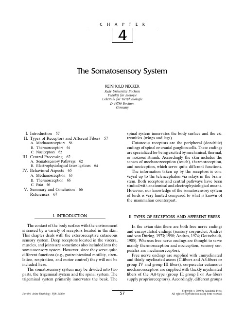
C H A P T E R4The Somatosensory SystemREINHOLD NECKERRuhr-Universita¨t BochumFakulta¨t fu¨r BiologieLehrstuhl fu¨r TierphysiologieD-44780BochumGermanyspinal system innervates the body surface and the ex-I.Introduction57tremities(wings and legs).II.Types of Receptors and Afferent Fibers57Cutaneous receptors are the peripheral(dendritic)A.Mechanoreceptors58B.Thermoreceptors61endings of spinal or cranial ganglion cells.These endingsC.Nociceptors62are specialized for being excited by mechanical,thermal, III.Central Processing62or noxious stimuli.Accordingly the skin includes theA.Somatosensory Pathways62senses of mechanoreception(touch),thermoreception,B.Electrophysiological Investigations64and nociception,which serve quite different functions. IV.Behavioral Aspects65The information taken up by the receptors is con-A.Mechanoreception65veyed up to the telencephalon via relays in the brain-B.Thermoreception66stem.Both receptors and central pathways have beenC.Pain66studied with anatomical and electrophysiological means. V.Summary and Conclusion66However,our knowledge of the somatosensory system References67of birds is very limited compared to what is known ofthe mammalian counterpart.I.INTRODUCTION II.TYPES OF RECEPTORS AND AFFERENT FIBERSThe contact of the body surface with the environment In the avian skin there are both free nerve endings is sensed by a variety of receptors located in the skin.and encapsulated endings(sensory corpuscles;Andres This chapter deals with the exteroreceptive cutaneous and von Du¨ring,1973;1990;Andres,1974;Gottschaldt, sensory system.Deep receptors located in the viscera,1985).Whereas free nerve endings are thought to serve muscles,and joints are sometimes also included into the mainly thermoreception and nociception,sensory cor-somatosensory system.However,since they serve quite puscles are mechanoreceptors.different functions(e.g.,gastrointestinal motility,circu-Free nerve endings are supplied with unmyelinated lation,respiration,and motor control)they will not be and thinly myelinated axons(C-ﬁbers and A␦-ﬁbers or included here.group IV and group IIIﬁbers),corpuscular cutaneous The somatosensory system may be divided into two mechanoreceptors are supplied with thickly myelinated parts,the trigeminal system and the spinal system.Theﬁbers of the Aͱ-type(group II;group I or AͰ-ﬁbers trigeminal system primarily innervates the beak.Thesupply proprioreceptors).Accordingly,different groupsCopyright᭧2000by Academic Press.57Sturkie’s Avian Physiology,Fifth Edition All rights of reproduction in any form reserved.58Reinhold Neckerofﬁber diameters and conduction velocities have been elmann and Myers,1961;Ostmann et al.,1963;Andres described(Necker and Meinecke,1984).C-ﬁbers haveand von Du¨ring,1990).There is a decreasing number ﬁber diameters of less than1Ȑm and conduction veloci-from head to tail to neck to wing with relatively few ties(CV)of less than2m/sec.A␦-ﬁbers have meancorpuscles on the back and fewest on the abdomen, diameters of about2Ȑm and mean CVs of about5m/andﬂying birds are supplied with a larger number than sec.There are two groups of large myelinated Aͱ-ﬁbersnonﬂying birds(Stammer,1961).which have mean diameters of about4and7Ȑm andb.Merkel Cell Receptorsmean CVs of about15and35m/sec,respectively.Merkel cell receptors of the avian skin share somesimilarity to the intraepidermal Merkel cell receptorsA.Mechanoreceptorsof mammals(Andres and von Du¨ring,1973).They are, Four main types of mechanosensitive sensory corpus-however,located in the dermis.The basic morphology cles may be distinguished in birds:Herbst corpuscles,of Merkel cell receptors is a Merkel cell and a disc-like Merkel cell receptors,Grandry corpuscles,and Rufﬁni axon ending contacting this cell(Merkel cell neurite endings.Although free nerve endings may function as complex;Figure1b).Merkel cells are characterized by mechanoreceptors(Iggo and Andres,1982),electro-their clear cytoplasm which typically contains dense-physiological evidence is lacking in birds.cored granula.Fingerlike processes interdigitate withthe surrounding Schwann cells.It is still a matter ofspeculation whether Merkel cells function as secondary 1.Morphology and Distribution ofsensory cells like hair cells in the inner ear.There are Cutaneous Mechanoreceptorssymmetrical membrane thickenings of the axon mem-a.Herbst Corpuscles brane and of the apposed Merkel cell membrane whichHerbst corpuscles are lamellated sensory receptorsresemble desmosomes rather than synaptic contacts comparable to the Pacinian corpuscles in mammals.The(Toyoshima and Shimamura,1991).ﬂattened axon ending is enlarged at its tip and is sur-Merkel cells may occur as single cells as well as in rounded by a central inner bulb(Figure1f).The inner groups and may even be organized as corpuscles with bulb cells are of Schwann cell origin and form two op-stacked arrangement similar to Grandry corpuscles of posing rows.The Schwann cell membrane adjacent to aquatic birds.Such corpuscles lack,however,a perineu-ral sheath.Merkel cells have been found predominantly the axon forms a complicated network of interdigitatedlamellae.Numerousﬁngerlike processes of the axon in the beak and tongue of various nonaquatic birds protrude into and form contacts with the lamellae.(Botezat,1906;Saxod,1978;Gentle and Breward,1986; These axon processes are thought to be the sites where Toyoshima and Shimamura,1991;Halata and Grim, the mechanical stimulus is tranduced into excitation of1993)but they have been described for the toe skin the sensory membrane(Gottschaldt et al.,1982).The(Ide and Munger,1978)and also for the feathered skin(Andres and von Du¨ring,1990).inner bulb is surrounded by a capsule space which con-tains cells of endoneural origin and collagenﬁbers whichc.Grandry Corpusclesform perforated concentric lamellae.The capsular spaceis enclosed by an outer capsule whose dense lamellae Grandry corpuscles occur in aquatic birds(anseri-are of perineural origin.The myelinated afferentﬁberforms)only(Gottschaldt,1985).As with Merkel cell looses its myelin sheath before entering the inner bulb.receptors there is an intimate contact between Grandry Herbst corpuscles are the most widely distributedcell and nerve ending.Grandry cells are thought to be receptors in the skin of birds.They are located in the of neural crest origin and are described as ganglion cell-deep dermis and they are found in the beak,in the legs,like.Typically two or more Grandry cells are stacked and in the feathered skin(Gottschaldt,1985).There is with discoid axon endings in between the cells(Figure a conspicuous assembly of sometimes more than one1a).There is an ongoing debate whether Grandry cells hundred Herbst corpuscles on the interosseous mem-and Merkel cells are two varieties of the same cell(Toy-brane of the leg(‘‘Herbstscher Strang’’[strand of Herbstoshima,1993).Grandry cells in aquatic birds are gener-corpuscles];Schildmacher,1931).In aquatic birds like ally larger than Merkel cells in nonaquatic birds.Except ducks and geese,in some shorebirds,and in the chickenfor size,Merkel cells and Grandry cells share most struc-there are bill tip organs with numerous Herbst corpus-tural specializations.Whereas Merkel cell corpuscles cles(Bolze,1968;Gottschaldt and Lausmann,1975;lack a sheath,Grandry corpuscles are always encapsu-Berkhoudt,1980;Gentle and Breward,1986).In feath-lated by a single-layered capsule of perineural origin. ered skin they are associated with the feather folliclesGrandry cells occur in the dermis of the bill of ducks and with muscles of the feathers(Stammer,1961;Wink-and geese(Saxod,1978;Berkhoudt,1980;GottschaldtChapter4.The Somatosensory System59FIGURE1Types of mechanoreceptors in the avian skin.(a)Grandry corpuscle of aquatic birds;(b)Merkelcell receptors;(c)Merkel cell corpuscle;(d)free stretch receptor ending;(e)Rufﬁni corpuscle;(f)Herbstcorpuscle.Abbreviations:c,capsule;cs,capsule space;cf,collagenﬁbers;di,disk-like afferent nerve ending;ef,efferentﬁber;m,Merkel cell;ps,perineural sheath;rax,receptor axon;sc,Schwann cell.After Andres(1974)with permission.and Lausmann,1974)and they are numerous in bill tip trophysiolocical(Reinke and Necker,1992a)but no organs,which are accumulations of sensory receptorsmorphological evidence of Rufﬁni endings in the feath-in connective tissueﬁlled channels of the horny premax-ered skin.illary plate of the bill.2.Electrophysiology of Mechanoreceptorsd.Rufﬁni EndingsElectrophysiologically mechanoreceptors have been Rufﬁni endings are well known and well studied inmammals but there are only few reports of this type of characterized by their response to a standard ramp-like mechanoreceptor in the avian skin.Rufﬁni corpusclesstimulus with a plateau(Figure2).There are rapidly are the encapsulated modiﬁcation of free stretch recep-adapting(RA)and slowly adapting(SA)responses tors(Figures1d and1e;Andres and von Du¨ring,1990).which may be further subdivided(Iggo and Gottschaldt, There is an extensive ramiﬁcation of the axon endings1974).Type SAI receptors respond both to the ramp which are in contact with bundles of collagenﬁbers.and to the plateau with a sustainedﬁring at irregular The contact zones are probably the tranducer sites.A spike intervals(random or Poisson distribution of inter-capsule consisting of layers of perineural cells may lackvals).This type of receptor may detect amplitudes of a in avian Rufﬁni endings(Gottschaldt,1985).stimulus(strength of touch or pressure).In mammals Rufﬁni endings have been identiﬁed so far only inthe morphological basis of this type of response is the the bill of geese(Gottschaldt et al.,1982)and in the intraepidermal Merkel cell receptor.Type SAII recep-beak of the Japanese quail(Halata and Grim,1993).tors also have a sustainedﬁring rate.However,there is There are,however,numerous Rufﬁni corpuscles in often spontaneous activity and a regularﬁring(normal joint capsules(Halata and Munger,1980).There is elec-or Gaussian distribution of intervals).In mammals the60Reinhold NeckerFIGURE2Types of responses of mechanoreceptors to a ramp-and-hold stimulus(uppermost trace).AfterIggo and Gottschaldt(1974)with permission.Rufﬁni corpuscle has been identiﬁed as an SAII receptor Leitner and Roumy,1974a;Ho¨rster,1990;Reinke and and the most effective stimulus consists of lateralNecker,1992b;Shen and Xu,1994).Thresholds are rather stretching of the skin.RA receptors respond to a change high below100Hz but decrease in the frequency range of stimulus intensity only,for example,during the ramp.300Hz up to1000Hz(Figure4).In the high-frequency Response varies with steepness(velocity of ramp).The range threshold amplitudes may be less than0.1Ȑm which morphological basis for these velocity detectors are theis in the range of human vibration sensitivity.Meissner corpuscles in glabrous skin and lanceolate end-The morphological basis of velocity-sensitive rapidly ings in hairy skin of mammals;neither type of receptoradapting responses is less clear although RA responses exists in birds.A very rapidly adapting type of response are very common.In the bill of aquatic birds RA re-shows spikes only at the beginning and/or end of thesponses are most likely based on Grandry corpuscles ramp;that is,during the acceleration phase of the ramp(Gottschaldt,1974).RA responses in the chicken beak stimulus.This type of receptor responds best to vibra-have been ascribed to Merkel cell(Grandry)corpuscles tion.The morphological basis of the vibration receptor(Gentle,1989).The morphological basis of RA re-in mammals is a lamellated corpuscle,the Pacinian cor-sponses in the feathered skin(Dorward,1970;Necker puscle.All types of responses have been observed in and Reiner,1980;Necker1985c,Reinke and Necker, birds also(Necker,1983;Gottschaldt,1985).However,1992a)is even less clear.Assuming,however,that avian the correlation of structure and function is less clear in Merkel cell receptors differ in location and hence in birds than in mammals.function from the mammalian counterpart(Andres and ThereisnodoubtthatHerbstcorpusclesarevibration-von Du¨ring,1990),and considering that there is a contin-sensitive receptors(Dorward,1970;Dorward and McIn-uum of rapidly adapting to slowly adapting responses tyre,1971;Gottschaldt,1974;Shen and Xu,1994).Vibra-(Dorward,1970;Necker,1985c),one might argue that tion receptors are usually characterized by strong phaseRA receptors in the feathered skin are due to Merkel coupling;that is,there is one spike per stimulus cycle.cell receptor activation.This means that avian Merkel In the cycle histogram it can be seen that the spikes ofcell receptors may have both rapidly adapting and slowly successive cycles fall within a limited phase angle range of adapting characteristics.the full360Њcycle(Figure3;Reinke and Necker,1992b).Both types of SA responses have been described in Herbst corpuscles are most sensitive to rather high fre-birds.SAI responses have most clearly been demon-quencies(Dorward and Mcintyre,1971;Gregory,1973;strated so far only in the feathered skin(Dorward,1970;Chapter4.The Somatosensory System61FIGURE4Dependence of threshold of vibration-sensitive afferentﬁbers in the interosseous nerve of the pigeon on vibration frequency.(After p.Physiol.A,Response characteristics of Herbst corpus-cles in the interosseous region of the pigeon’s hind limb,J.X.Shenand Z.M.Xu,175,667–674,Fig.7,1994,᭧Springer-Verlag.)and Fedde,1993).These receptors increase activity withincreasing elevation of covert feathers.FIGURE3Response of a vibration-sensitive afferentﬁber.(a)Origi-B.Thermoreceptorsnal traces of action potentials(above)and a300-Hz vibration stimulus(below).(b)Cycle histogram of the same recording shows the occur-Thermoreceptors are thought to be free nerve end-ence of action potentials at a distinct phase of the stimulus cycle(0Њings(Hensel,1973).This seems to hold for avian ther-to360Њ).(After p.Physiol.A,Spinal dorsal column afferentﬁber composition in the pigeon:An electrophysiological investigation,moreceptors also since the conduction velocity of ther-H.Reinke and R.Necker,171,397–403,1992,᭧Springer-Verlag.)moreceptive afferents has been shown to be in the rangeof A␦-and C-ﬁbers(mean:2m/sec;Gentle1989).Ther-moreceptors are characterized by spontaneous activity Necker1985c;Brown and Fedde,1993).Response char-at normal skin temperature which increases during cool-acteristics are very similar to those of mammalian Merkel ing(cold receptors)or during warming(warm recep-cell receptors.This includes a high dynamic sensitivity tors).Typically,rapid temperature changes result in an during mechanical stimulation and cold sensitivity excitatory overshoot.Thermoreceptors in the avian skin (Necker,1985c).The location nearﬁloplume follicles(mainly beak and tongue)have been described repeat-(Necker,1985c)agrees with the anatomical demonstra-edly(Kitchell et al.,1959;Leitner and Roumy,1974b; tion of groups of Merkel cells in the follicle wall(Andres Gregory,1973;Necker,1972,1973;Gentle,1987,1989; and von Du¨ring,1990).Scha¨fer et al.,1989).Mostﬁbers were cold afferents and Type SAII responses seem to be common in the beak there are only few demonstrations of warm receptors skin(Necker,1974a,b;Gottschaldt,1974;Gottschaldt(Necker,1972,1973;Gentle,1987,1989).et al.,1982)and the Rufﬁni endings are most likely Both the dynamic overshoot and the static tempera-the morphological basis(Gottschaldt et al.,1982).SAII ture-dependent activity of cold receptors in the beakreponses have been observed in the feathered skin of and tongue is lower than in mammalian cold receptorsthe pigeon also,and the most effective stimulus was(Figures5and6).As in mammals there is a maximumlateral stretch of skin,as in mammals(Reinke and static and dynamic activity at about25Њto30ЊC.ThereNecker,1992a).SA responses of unclear origin(proba-is more indirect(Necker,1977)than direct evidence ofbly Rufﬁni endings or free stretch receptors)have been cold sensitivity of the feathered skin(Necker anddescribed with wing afferents in the chicken(BrownReiner,1980;Necker,1985b).Spontaneous activity of62Reinhold NeckerFIGURE5Activity of cold receptor neurons in the trigeminal gan-glion of the pigeon.(A)Response to cooling steps(temperature asindicated):(B)dependence of static activity of sixﬁbers on adaptingtemperature.(After Scha¨fer et al.(1989),Brain Res.501,66–72,withpermission from Elsevier Science.)FIGURE6Dependence of activity of a cold receptor(a)and of awarm receptor(b)on beak skin temperature in the pigeon.Originalspike traces on the left and static activity on the right.(After J. warm receptors is high and there is an increase of staticComp.Physiol.A,Response of trigeminal ganglion neurons to thermalstimulation of the beak of pigeons,R.Necker,78,307–314,1972,᭧activity with increasing temperature in the range of25ЊSpringer-Verlag.)to45ЊC(Figure6).C.Nociceptors III.CENTRAL PROCESSINGNociceptors respond to stimuli which threaten todamage the skin.Both mechanical stimuli(pin prick, A.Somatosensory Pathways squeezing)and thermal stimuli(heat above about45ЊC)1.Trigeminal Systemare effective in exciting nociceptor afferents.Differenttypes of nociceptors have been described:high threshold The trigeminal nerve consists of three branches,the mechanoreceptors,heat nociceptors,and polymodal ramus ophthalmicus,which innervates the orbita,the nociceptors(activated by heat,mechanical stimuli,and nasal area,and rostral part of the upper beak;the ramus chemical agents like bradykinin;Burgess and Perl,maxillaris,which innervates the upper beak;and the1973).All of these types seem to occur both in theramus mandibularis which innervates the lower beak. feathered skin(Necker and Reiner,1980)and in theThe ophthalmic nerve and the maxillary nerve are pure beak skin(Gentle,1989).sensory nerves whereas the mandibular nerve is a mixed Nociceptors have no or only little spontaneous activ-sensory and motor nerve(Barnikol,1953).Sensory com-ity.High-threshold(nociceptive)mechanoreceptors in-ponents of the facial nerve and the glossopharyngeal crease activity with increasing force of mechanical stim-nerve may join the trigeminal system(Dubbeldam et al., ulation(Figure7a).Heat nociceptors increase activity1979;Dubbeldam,1984a;Bout and Dubbeldam,1985). when skin temperature exceeds about45ЊC,and thereThe somata of the trigeminal nerve are located in is an increasing activation up to temperatures abovethe trigeminal ganglion(g.gasseri).The central root 50ЊC(Figure7b).All of these responses show slow adap-enters the brainstem and afferentﬁbers either ascend tation.Nociceptors seem to be quite numerous both inin the ascending trigeminal tract(TTA),which ends in the beak skin and in the feathered skin(Necker andReiner,1980;Gentle,1989).the main sensory nucleus of theﬁfth cranial nerve(PrV,Chapter4.The Somatosensory System63FIGURE8Schematic outline of central pathways of the trigeminalsystem.Afferents to the trigeminal nuclei on the left side of the brain,efferents on the right side.Bas,nucleus basalis;cd,pars caudalis ofthe descending trigeminal system(TTD);dh,cervical dorsal horn;G,trigeminal ganglion;ip,pars interpolaris of TTD,or,pars oralis ofTTD;PrV,nucleus principalis nervi trigemini;rf,projection to thereticular formation;th,projection to the thalamus.(After Dubbeldam(1984b)with permission from S.Karger AG,Basel.)dam,1984).Pars oralis is the only trigeminal nucleus toproject to the cerebellum(Arends et al.,1984;Arendsand Zeigler,1989).Pars interpolaris has mainly intra-nuclear connections to oralis and PrV.Pars caudalis andcervical dorsal horn may project up to the thalamus,joining the medial lemniscus(Arends el al.,1984).Themore caudal subnuclei have projections to the neighbor-ing reticular formation which may be important for mo-FIGURE7Dependence of activity of nociceptors on increasing tor control(see Chapter6).force(a)and increasing temperature(b).(After p.Physiol.It has long been known that PrV projects via the A,Cutaneous sensory afferents recorded from the nervus intraman-quintofrontal tract to the nucleus basalis(Bas)or nu-dibularis of Gallus gallus var.domesticus,M.J.Gentle,164,763–774,cleus prosencephali trigeminalis of the telencephalon, 1989,᭧Springer-Verlag.)bypassing the thalamus(Cohen and Karten,1974).There is both an ipsilateral and a contralateral projec-tion and in the mallard a topographic representation of nucleus principalis nervi trigemini),or descend in thethe branches of the trigeminal nerve could be demon-descending trigeminal tract(TTD),which extends cau-strated(Dubbeldam et al.,1981,Figure8).Nucleus ba-dally to the upper spinal cervical segments(Karten andsalis projects to the nearby frontal neostriatum which Hodos,1967;Dubbeldam and Karten,1978;Dubbel-seems to be at the origin of a network connecting the dam,1980).In the pigeon there is a lateral componentbeak sensory system to the motor system,a circuit im-of TTD(lTTD)which mainly terminates in the externalportant for feeding(see Chapter6).cuneate nucleus of the medulla.There is a somatotopicprojection of the three divisions of the trigeminal nerveto PrV in such a way that the mandibular branch projects 2.Spinal Systemdorsally,the maxillary branch intermedially,and theWhereas the peripheral branches of spinal ganglion ophthalmic branch ventrally.cells innervate receptors in the periphery the central The TTD is accompanied by the nucleus of the TTDbranches enter the spinal cord by the dorsal root.Collat-(nTTD)which can be devided into several subnucleierals either ascend in the dorsal column or terminate from rostral to caudal:pars oralis(or)near PrV,parsin the grey substance(for details of the spinal cord see interpolaris(ip),pars caudalis(cd),and spinal dorsalhorn(dh)in the upper cervical spinal cord(Figure8).In Chapter5).the nTTDﬁbers of the three branches of the trigeminalThere are several ascending pathways in the spinal nerve terminate in a topographic order in all subnuclei cord.The main pathways described for the mammalian (Dubbeldam and Karten,1978;Arends and Dubbel-spinal cord(dorsal column,spinoolivary,spinocerebellar,64Reinhold Neckerspinoreticular,spinomesencephalic,and spinothalamic)solateralis posterior(DLP).There is a differential pro-are found in the bird also(see Chapter5).However,therejection of GC and CE whose signiﬁcance is unknown as is only sparse direct projection to the thalamus.yet(Wild,1989).The same thalamic targets are reached The dorsal column pathway(mechanoreception)isby spinal afferents(Schneider and Necker,1989). outlined in Figure9.Primary afferentﬁbers ascend in The thalamic somatosensory nuclei have different the dorsal column to terminate in the dorsal columnipsilateral projections to the telencephalon.The DLP nuclei(nuclei gracilis et cuneatus,GC;nucleus cuneatus projects to a somatosensory area in the medial caudal externus,CE)of the medulla oblongata(van den Akker,neostriatum(NC)near the auditoryﬁeld L(see hearing 1970;Wild,1985;Necker and Schermuly,1985;Schulte Chapter2)and to the rostrally adjacent intermediateneostriatum(NI).The NC further projects to the overly-and Necker,1994).The medially located nucleus gracilis(leg afferents)and the laterally located nucleus cuneatus ing hyperstriatum ventrale(HV;Funke,1989b).The (wing afferents)can be separated in caudal parts of themain thalamic projection is from DIVA to a somatosen-medulla only and there is an overlapping projection in sory area far rostral in the telencephalon in the Wulst, rostral GC and in the external cuneate nucleus(van dena rostromedial bulge in the avian telencephalon.The Akker,1970;Wild,1985).The CE does not correspond rostral part of the Wulst serves somatosensory represen-tation whereas the caudal part serves vision.This part to the mammalian analog(no relay of forelimb musclespindle afferents).In addition to the primary afferent of the brain belongs to the hyperstriatum accessorium ﬁbers there are secondary afferents from laminae IV(HA)and it is the intermediate part(IHA)which re-and V neurons of the dorsal horn(see Chapter5).ceives DIVA afferents(Wild,1987;Funke,1989b).Both The dorsal column nuclei all project to the thalamustelencephalic areas are interconnected(Figure9).Both via the medial lemniscus.There is a crossed and a spinal somatosensory representation areas have connec-tions to descending(motor)systems(see Chapter6). smaller uncrossed pathway andﬁbers give off collateralsto the inferior olive,to the intercollicular area ventraland medial to the auditory nucleus mesencephali later-B.Electrophysiological Investigationsalis pars dorsalis(MLD),and to nucleus spiriformesmedialis(Wild,1989).The main somatosensory thala- 1.Thermoreception and Nociceptionmic nucleus has now been identiﬁed as the nucleus dor-Nociception and thermoreception have been studied salis intermedius ventralis anterior(DIVA)ﬁrst de-so far only in the spinal dorsal horn.As in mammals, scribed in the owl(Karten et al.,1978)and thennociceptive and thermoreceptive neurons are mainly conﬁrmed in the pigeon(Wild,1987;Funke,1989b;found in lamina I of the spinal dorsal horn both of the Schneider and Necker,1989).A smaller contingent ofcervical and of the lumbar enlargements(Necker,1985b; dorsal column nuclei afferents reaches the nucleus dor-Woodbury,1992).There is no signiﬁcant direct projec-tion of these neurons to the thalamus(see Chapter5).However,thermoreceptive and nociceptive informationmay reach higher levels of the brain via relays in thebrainstem reticular formation(Necker,1989;Gu¨ntherand Necker,1995).2.Mechanoreceptiona.Trigeminal System and Beak RepresentationIn the trigeminal system the beak is represented bothin PrV and in nTTD.In both nuclei a dorsoventralsomatotopic organization has been conﬁrmed with elec-trophysiological recordings in the pigeon(Zeigler andWitkovsky,1968;Silver and Witkovsky,1973).Unitswere rapidly adapting or slowly adapting and some re-sponded to opening and/or closing the beak.Tongue FIGURE9Schematic outline of central pathways of the mechanore-stimulation was ineffective which conﬁrms the lack of ceptive spinal system.Bas,nucleus basalis;DH,dorsal horn;DIVA,glossopharyngeal projections to the trigeminal systemnucl.dorsalis intermedius ventralis anterior;DLP,nucleus dorsolater-in the pigeon(Dubbeldam,1984a).alis posterior;GC/CE,nuclei gracilis et cuneatus/nucleus cuneatusThere is evidence of responses of neurons in the so-externus;HA,hyperstriatum accessorius;ICo,nucleus intercollicu-laris;NC,neostriatum caudale;OI,oliva inferior.matosensory thalamus to beak stimulation(Delius andChapter4.The Somatosensory System65 Bennetto,1972;Witkovsky et al.,1973)and it seems that somatosensory relay(Korzeniewska1987;Korzeniew-DLP is the main site of thalamic beak representationska and Gu¨ntu¨rku¨n,1989).A detailed analysis showed (Korzeniewska,1987).Because of the lack of collaterals that most DIVA neurons respond speciﬁcally to bodystimulation(Schneider and Necker,1996).Receptive from the quintofrontal tract this information may reachthe thalamus via the descending trigeminal system.ﬁelds were often large,normally covering the whole ex-Processing in the nucleus basalis has been studiedtremity and some including both extremities.The small-both in the pigeon and in the mallard.In both species est receptiveﬁelds were located on the toes.A somato-receptiveﬁelds were often rather small especially at thetopic organization was largely missing although the area tip of the beak and there was a somatotopic organization with predominant wing responses could be separatedfrom a more rostral area with predominant leg responses. (Figure8;Witkovsky et al.,1973;Berkhoudt et al.,1981).The tongue was represented in the mallard but not in The telencephalic areas(NC/NI/HV,IHA)were the pigeon as expected from the anatomical studies.Instudied at the single-unit level(Funke,1989a).Both contrast to PrV all units showed rapid adaptation.areas disclosed poor somatotopic organization.Re-In sandpipers and snipes(family Scolopacidae)anceptiveﬁelds were smaller in IHA than in NC.Accord-enormous enlargement of nucleus basalis forming a ingly,there was a faint somatotopy in the Wulst(HA)area with rostral parts of the body being represented bulge on the basolateral surface of the brain has beenobserved(Pettigrew and Frost,1985).Electrophysiolog-superﬁcially and caudal parts in deeper layers.In the ical recordings revealed an overrepresentation of theowl a detailed representation of the toes was found in bill tip.By analogy to the fovea in the eye a tactile fovea the Wulst area(Karten et al.,1978).There was has been postulated for these birds.no somatotopic representation of the body in theNC/NI and adjacent HV and bimodal input(auditory/ b.Spinal System and Body Representation somatosensory)was common in this caudal area(Funke,1989a).These differences in the two areas suggest that The spinal dorsal horn has been studied electrophysi-the HA area may be compared to SI and NC/NI to SII of ologically in detail in the pigeon cervical enlargementthe mammalian somatosensory cortical representations. (Necker,1985a,b,1990)and in the chicken lumbosacralenlargement(Woodbury,1992).There is a somatotopicorganization similar to that in mammals;for example,IV.BEHAVIORAL ASPECTSdistal parts of the extremities are represented mediallyand proximal parts laterally(see Chapter5).A.MechanoreceptionMechanoreceptive neurons are located in lamina IVof the dorsal horn both in the pigeon and in the chicken.Cutaneous mechanoreceptors are involved in a vari-Both slowly adapting and rapidly adapting responses ety of behavioral responses.Most evident is a contribu-have been observed but there is no clear evidence of tion of beak receptors to feeding(see Chapter6).In input from Herbst corpuscles in the cervical cord of the this context it has to be kept in mind that the avian pigeon although it seems to be present in the lumbosa-beak serves as a prehensile organ comparable to the cral enlargement of the chicken.In the ascending dorsal human hand.Parrots and birds of prey use both feet column many primary afferentﬁbers respond to vibra-and beak for the handling of food items.Interestingly tory stimuli(Reinke and Necker,1992b).both beak and feet(toes)are the only parts of the avian In the dorsal column nuclei there is evidence for a body which are represented in great detail in the CNS. separate representation of leg and wing at least in caudal In the feet the conspicuous strand of Herbst corpus-parts of these nuclei(Necker,1991).Many neurons in cles on the interosseous membrane is exquisitely suit-the GC show Herbst corpuscle input and there are also able to detect vibrations of the ground(Schwartzkopff, slowly adapting responses(Reinke and Necker,1996).1949),perhaps even earthquakes(Shen and Xu,1994). CE seems to process primarily deep input(joint recep-Mechanoreceptors in the feathered skin can detect tors).However,input from muscle spindles was not disorders of the plumage(Necker,1985a).This may found.Together with theﬁnding that the CE does not trigger preening although this behavior does not neces-project to the cerebellum(Wild,1989)this supports the sarily depend on sensory input(Delius,1988).Vibra-assumption that the avian CE is not homologous to the tions of the plumage occur duringﬂight and mechanore-mammalian external cuneate nucleus.ceptors may detect turbulences in the air stream and Delius and Bennetto(1972)were theﬁrst to record in this way inﬂuenceﬂight control.Air stream evoked somatosensory responses from the avian thalamus in the stimulation of mechanoreceptors in the feathered skin DLP/DIVA region.Whereas the DLP turned out to be a is important forﬂight pattern(Gewecke and Woike, multimodal nucleus processing both somatosensory and1978)and forﬂight reﬂexes(Bilo and Bilo,1978).It is visual and auditory stimuli DIVA seems to be a speciﬁcinteresting that information from feather mechanore-。

船舶专业外文文献

Spatial scheduling for large assemblyblocks in shipbuilding令狐采学Abstract: This paper addresses the spatial scheduling problem (SPP) for large assembly blocks, which arises in a shipyard assembly shop. The spatial scheduling problem is to schedule a set of jobs, of which each requires its physical space in a restricted space. This problem is complicated because both the scheduling of assemblies with different due dates and earliest starting times and the spatial allocation of blocks with different sizes and loads must be considered simultaneously. This problem under consideration aims to the minimization of both the makespan and the load balance and includes various real-world constraints, which includes the possible directional rotation of blocks, the existence of symmetric blocks, and the assignment of some blocks to designated workplaces or work teams. The problem is formulated as a mixed integer programming (MIP) model and solved by a commercially available solver. A two-stage heuristic algorithm has been developed to use dispatching priority rules and a diagonal fill space allocation method, which is a modification of bottom-left-fill space allocation method. Thecomparison and computational results shows the proposed MIP model accommodates various constraints and the proposed heuristic algorithm solves the spatial scheduling problems effectively and efficiently.Keywords:Large assembly block; Spatial scheduling; Load balancing; Makespan; Shipbuilding1. IntroductionShipbuilding is a complex production process characterized by heavy and large parts, various equipment, skilled professionals, prolonged lead time, and heterogeneous resource requirements. The shipbuilding process is divided into sub processes in the shipyard, including ship design, cutting and bending operations, block assembly, outfitting, painting, pre-erection and erection. The assembly blocks are called the minor assembly block, the sub assembly block, and the large assembly block according to their size and progresses in the course of assembly processes. This paper focuses on the spatial scheduling problem of large assembly blocks in assembly shops. Fig. 1 shows a snapshot of large assembly blocks in a shipyard assembly shop.Recently, the researchers and practitioners at academia and shipbuilding industries recently got together at “Smart Production Technology Forum in Shipbuilding and Ocean Plant Industries” to recognize that there are various spatial scheduling problems in everyaspect of shipbuilding due to the limited space, facilities, equipment, labor and time. The SPPs occur in various working areas such as cutting and blast shops, assembly shops, outfitting shops, pre-erection yard, and dry docks. The SPP at different areas has different requirements and constraints to characterize the unique SPPs. In addition, the depletion of energy resources on land put more emphasis on the ocean development. The shipbuilding industries face the transition of focus from the traditional shipbuilding to ocean plant manufacturing. Therefore, the diversity of assembly blocks, materials, facilities and operations in ship yards increases rapidly.There are some solution providers such as Siemens™ and DassultS ystems™ to provide integrated software including product life management, enterprise resource planning system, simulation and etc. They indicated the needs of efficient algorithms to solve medium- to large-sized SPP problems in 20 min, so that the shop can quicklyre-optimize the production plan upon the frequent and unexpected changes in shop floors with the ongoing operations on exiting blocks intact.There are many different applications which require efficient scheduling algorithms with various constraints and characteristics (Kim and Moon, 2003, Kim et al., 2013, Nguyen and Yun,2014 and Yan et al., 2014). However, the spatial scheduling problemwhich considers spatial layout and dynamic job scheduling has not been studied extensively. Until now, spatial scheduling has to be carried out by human schedulers only with their experiences and historical data. Even when human experts have much experience in spatial scheduling, it takes a long time and intensive effort to produce a satisfactory schedule, due to the complexity of considering blocks’ geometric shapes, loads, required facilities, etc. In practice, spatial scheduling for more than a six-month period is beyond the human schedulers’ capacity. Moreover, the space in the working areas tends to be the most critical resource in shipbuilding. Therefore, the effective management of spatial resources through automation of the spatial scheduling process is a critical issue in the improvement of productivity in shipbuilding plants.A shipyard assembly shop is consisted of pinned workplaces, equipment, and overhang cranes. Due to the heavy weight of large assembly block, overhang cranes are used to access any areas over other objects without any hindrance in the assembly shop. The height of cranes can limit the height of blocks that can be assembled in the shop. The shop can be considered as a two-dimensional space. The blocks are placed on precisely pinned workplaces.Once the block is allocated to a certain area in a workplace, it is desirable not to move the block again to different locations due to thesize and weight of the large assembly blocks. Therefore, it is important to allocate the workspace to each block carefully, so that the workspace in an assembly shop can be utilized in a most efficient way. In addition, since each block has its due date which ispre-determined at the stage of ship design, the tardiness of a block assembly can lead to severe delay in the following operations. Therefore, in the spatial scheduling problem for large assembly blocks, the scheduling of assembly processes for blocks and the allocation of blocks to specific locations in workplaces must be considered at the same time. As the terminology suggests, spatial scheduling pursues the optimal spatial layout and the dynamic schedule which can also satisfy traditional scheduling constraints simultaneously. In addition, there are many constraints or requirements which are serious concerns on shop floors and these complicate the SPP. The constraints or requirements this study considered are explained here: (1) Blocks can be put in either directions, horizontal or vertical. (2) Since the ship is symmetric around the centerline, there exist symmetric blocks. These symmetric blocks are required to be put next to each other on the same workplace. (3) Some blocks are required to be put on a certain special area of the workplace, because the work teams on that area has special equipment or skills to achieve a certain level of quality or complete the necessary tasks. (4) Frequently, the production plan may not be implemented as planned, so that frequentmodifications in production plans are required to cope with the changes in the shop. At these modifications, it is required to produce a new modified production plan which does not remove or move the pre-existing blocks in the workplace to complete the ongoing operations. (5) If possible at any time, the load balancing over the work teams, i.e., workplaces are desirable in order to keep all task assignments to work teams fair and uniform.Lee, Lee, and Choi (1996) studied a spatial scheduling that considers not only traditional scheduling constraints like resource capacity and due dates, but also dynamic spatial layout of the objects. They used two-dimensional arrangement algorithm developed by Lozano-Perez (1983) to determine the spatial layout of blocks in shipbuilding. Koh, Park, Choi, and Joo (1999) developed a block assembly scheduling system for a shipbuilding company. They proposed a two-phase approach that includes a scheduling phase and a spatial layout phase. Koh, Eom, and Jang (2008) extended their precious works (Koh et al., 1999) by proposing the largest contact area policy to select a better allocation of blocks. Cho, Chung, Park, Park, and Kim (2001) proposed a spatial scheduling system for block painting process in shipbuilding, including block scheduling, four arrangement algorithms and block assignment algorithm. Park et al. (2002) extended Cho et al. (2001) utilizing strategy simulation in two consecutive operations ofblasting and painting. Shin, Kwon, and Ryu (2008) proposed a bottom-left-fill heuristic method for spatial planning of block assemblies and suggested a placement algorithm for blocks by differential evolution arrangement algorithm. Liu, Chua, and Wee (2011) proposed a simulation model which enabled multiple priority rules to be compared. Zheng, Jiang, and Chen (2012) proposed a mathematical programming model for spatial scheduling and used several heuristic spatial scheduling strategies (grid searching and genetic algorithm). Zhang and Chen (2012) proposed another mathematical programming model and proposed the agglomeration algorithm.This study presents a novel mixed integer programming (MIP) formulation to consider block rotations, symmetrical blocks,pre-existing blocks, load balancing and allocation of certain blocks to pre-determined workspace. The proposed MIP models were implemented by commercially available software, LINGO® and problems of various sizes are tested. The computational results show that the MIP model is extremely difficult to solve as the size of problems grows. To efficiently solve the problem, a two-stage heuristic algorithm has been proposed.Section 2 describes spatial scheduling problems and assumptions which are used in this study. Section 3 presents a mixed integerprogramming formulation. In Section 4, a two-stage heuristic algorithm has been proposed, including block dispatching priority rules and a diagonal fill space allocation heuristic method, which is modified from the bottom-left-fill space allocation method. Computational results are provided in Section 5. The conclusions are given in Section 6.2. Problem descriptionsThe ship design decides how to divide the ship into many smaller pieces. The metal sheets are cut, blast, bend and weld to build small blocks. These small blocks are assembled to bigger assembly blocks. During this shipbuilding process, all blocks have their earliest starting times which are determined from the previous operational step and due dates which are required by the next operational step. At each step, the blocks have their own shapes of various sizes and handling requirements. During the assembly, no block can overlap physically with others or overhang the boundary of workplace.The spatial scheduling problem can be defined as a problem to determine the optimal schedule of a given set of blocks and the layout of workplaces by designating the blocks’ workplace simultaneously. As the term implies, spatial scheduling pursues the optimal dynamic spatial layout schedule which can also satisfy traditional scheduling constraints. Dynamic spatial layout schedule can be including thespatial allocation issue, temporal allocation issue and resource allocation issue.An example of spatial scheduling is given in Fig. 2. There are 4 blocks to be allocated and scheduled in a rectangular workplace. Each block is shaded in different patterns. Fig. 2 shows the 6-day spatial schedule of four large blocks on a given workplace. Blocks 1 and 2 arepre-existed or allocated at day 1. The earliest starting times of blocks 3 and 4 are days 2 and 4, respectively. The processing times of blocks 1, 2 and 3 are 4, 2 and 4 days, respectively.The spatial schedule must satisfy the time and space constraints at the same time. There are many objectives in spatial scheduling, including the minimization of makespan, the minimum tardiness, the maximum utilization of spatial and non-spatial resources and etc. The objective in this study is to minimize the makespan and balance the workload over the workspaces.There are many constraints for spatial scheduling problems in shipbuilding, depending on the types of ships built, the operational strategies of the shop, organizational restrictions and etc. Some basic constraints are given as follows; (1) all blocks must be allocated on given workplaces for assembly processes and must not overstep the boundary of the workplace; (2) any block cannot overlap with other blocks; (3) all blocks have their own earliest starting time and duedates; (4) symmetrical blocks needs to be placed side-by-side in the same workspace. Fig. 3 shows how symmetrical blocks need to be assigned; (5) some blocks need to be placed in the designated workspace; (6) there can be existing blocks before the planning horizon; (7) workloads for workplaces needs to be balanced as much as possible.In addition to the constraints described above, the following assumptions are made.(1)The shape of blocks and workplaces is rectangular.(2)Once a block is placed in a workplace, it cannot be moved or removed from its location until the process is completed.(3)Blocks can be rotated at angles of 0° and 90° (see Fig. 4).(4)The symmetric blocks have the same sizes, are rotated at the same angle and should be placed side-by-side on the same workplace. (5)The non-spatial resources (such as personnel or equipment) are adequate.3. A mixed integer programming modelA MIP model is formulated and given in this section. The objective function is to minimize makespan and the sum of deviation from average workload per workplace, considering the block rotation, the symmetrical blocks, pre-existing blocks, load balancing and theallocation of certain blocks to pre-determined workspace.A workspace with the length LENW and the width WIDW is considered two-dimensional rectangular space. Since the rectangular shapes for the blocks have been assumed, a block can be placed on workspace by determining (x, y) coordinates, where 0 ⩽ x ⩽ LENW and 0 ⩽ y ⩽ WIDW. Hence, the dynamic layout of blocks on workplaces is similar to two-dimensional bin packing problem. In addition to the block allocation, the optimal schedule needs to be considered at the same time in spatial scheduling problems. Z axis is introduced to describe the time dimension. Then, spatial scheduling problem becomes a three-dimensional bin packing problem with various objectives and constraints.The decision variables of spatial scheduling problem are (x, y, z) coordinates of all blocks within a three-dimensional space whose sizes are LENW, WIDW and T in x, y and z axes, where T represents the planning horizon. This space is illustrated in Fig. 5.In Fig. 6, the spatial scheduling of two blocks into a workplace is illustrated as an example. The parameters p1 and p2 indicate the processing times for Blocks 1 and 2, respectively. As shown in z axis, Block 2 is scheduled after Block 1 is completed.4. A two-stage heuristic algorithmThe computational experiments for the MIP model in Section 3 have been conducted using a commercially available solver, LINGO®. Obtaining global optimum solutions is very time consuming, considering the number of variables and constraints. A ship is consisted of more than 8 hundred large blocks and the size of problem using MIP model is beyond today’s computational ability.A two-stage heuristic algorithm has been proposed using the dispatching priority rules and a diagonal fill method.4.1. Stage 1: Load balancing and sequencingPast research on spatial scheduling problems considers various priority rules. Lee et al. (1996) used a priority rule for the minimum slack time of blocks. Cho et al. (2001) and Park et al. (2002) used the earliest due date. Shin et al. (2008) considered three dispatching priority rules for start date, finish date and geometric characteristics (length, breadth, and area) of blocks. Liu and Teng (1999) compared 9 different dispatching priority rules including first-come first-serve, shortest processing time, least slack, earliest due date, critical ratio, most waiting time multiplied by tonnage, minimal area residue, and random job selection. Zheng et al. (2012) used a dispatching rule of longest processing time and earliest start time.Two priority rules are used in this study to divide all blocks into groups for load balancing and to sequence them considering the duedate and earliest starting time. Two priority rules are streamlined to load-balance and sequence the blocks into an algorithm which is illustrated in Fig. 7. The first step of the algorithm in this stage is to group the blocks based on the urgency priority. The urgency priority is calculated by subtracting the earliest starting time and the processing time from the due date for each block. The smaller the urgency priority, the more urgent the block needs to bed scheduled. Then all blocks are grouped into an appropriate number of groups for a reasonable number of levels in urgency priorities. Let g be this discretionary number of groups. There are g groups of blocks based on the urgency of blocks. The number of blocks in each group does not need to be identical.Blocks in each group are re-ordered grouped into as many subgroups as workplaces, considering the workload of blocks such as the weight or welding length. The blocks in each subgroup have the similar urgency and workloads. Then, these blocks in each subgroup are ordered in an ascending order of the earliest starting time. This ordering will be used to block allocations in sequence. The subgroup corresponds to the workplace.If block i must be processed at workplace w and is currently allocated to other workplace or subgroup than w, block i is swapped with a block at the same position of block i in an ascending order of theearliest starting time at its workplace (or subgroup). Since the symmetric blocks must be located on a same workplace, a similar swapping method can be used. One of symmetric blocks which are allocated into different workplace (or subgroups) needs to be selected first. In this study, we selected one of symmetric blocks whichever has shown up earlier in an ascending order of the earliest starting time at their corresponding workplace (or subgroup). Then, the selected block is swapped with a block at the same position of symmetric blocks in an ascending order of the earliest starting time at its workplace (or subgroups).4.2. Stage 2: Spatial allocationOnce the blocks in a workplace (or subgroup) are sequentially ordered in different urgency priority groups, each block can be assigned to workplaces one by one, and allocated to a specific location on a workplace. There has been previous research on heuristic placement methods. The bottom-left (BL) placement method was proposed by Baker, Coffman, and Rivest (1980) and places rectangles sequentially in a bottom-left most position. Jakobs (1996) used a bottom-left method that is combined with a hybrid genetic algorithm (see Fig. 8). Liu and Teng (1999) developed an extended bottom-left heuristic which gives priority to downward movement, where the rectangles is only slide leftwards if no downward movement is possible. Chazele(1983) proposed the bottom-left-fill (BLF) method, which searches for lowest bottom-left point, holes at the lowest bottom-left point and then place the rectangle sequentially in that bottom-left position. If the rectangle is not overlapped, the rectangle is placed and the point list is updated to indicate new placement positions. If the rectangle is overlapped, the next point in the point list is selected until the rectangle can be placed without any overlap. Hopper and Turton (2000) made a comparison between the BL and BLF methods. They concluded that the BLF method algorithm achieves better assignment patterns than the BL method for Hopper’s example problems. Spatial allocation in shipbuilding is different from two-dimensional packing problem. Blocks have irregular polygonal shapes in the spatial allocation and blocks continuously appear and disappear since they have their processing times. This frequent placement and removal of blocks makes BLF method less effective in spatial allocation of large assembly block.In order to solve these drawbacks, we have modified the BLF method appropriate to spatial scheduling for large assembly blocks. In a workplace, since the blocks are placed and removed continuously, it is more efficient to consider both the bottom-left and top-right points of placed blocks instead of bottom-left points only. We denote it as diagonal fill placement (see Fig. 9). Since the number of potentialplacement considerations increases, it takes a bit more time to implement diagonal fill but the computational results shows that it is negligible.The diagonal fill method shows better performances than the BLF method in spatial scheduling problems. When the BLF method is used in spatial allocation, the algorithm makes the allocation of some blocks delayed until the interference by pre-positioned blocks are removed. It generates a less effective and less efficient spatial schedule. The proposed diagonal fill placement method resolve this delays better by allocating the blocks as soon as possible in a greedy way, as shown in Fig. 10. The potential drawbacks from the greedy approaches is resolved by another placement strategy to minimize the possible dead spaces, which will be explained in the following paragraphs.The BLF method only focused on two-dimensional bin packing. Frequent removal and placement of blocks in a workspace may lead to accumulation of dead spaces, which are small and unusable spaces among blocks. A minimal possible-dead space strategy has been used along with the BLF method. Possible-dead spaces are being generated over the spatial scheduling and they have less chance to be allocated for future blocks. The minimal possible-dead space strategy minimizes the potential dead space after allocating the followingblocks (Chung, 2001 and Koh et al., 2008) by considering the 0° and 90° rotation of the block and allocating the following block for minimal possible-dead space. Fig. 11 shows an example of three possible-dead space calculations using the neighbor block search method. When a new scheduling block is considered to be allocated, the rectangular boundary of neighboring blocks and the scheduling blocks is searched. This boundary can be calculated by obtaining the smallest and the largest x and y coordinates of neighboring blocks and the scheduling blocks. Through this procedure, the possible-dead space can be calculated as shown in Fig. 11. Considering the rotation of the scheduling blocks and the placement consideration points from the diagonal fill placement methods, the scheduling blocks will be finally allocated.In this two-stage algorithm, blocks tend to be placed adjacent to one of the alternative edges and their assignments are done preferentially to minimize fractured spaces.5. Computational resultsTo demonstrate the effectiveness and efficiency of the proposed MIP formulation and heuristic algorithm, the actual data about 800+ large assembly blocks from one of major shipbuilding companies has been obtained and used. All test problems are generated from thisreal-world data.All computational experiments have been carried out on a personal computer with a Intel® Core™ i3*********************** RAM. The MIP model in Section 3 has been programmed and solved using LINGO® version 10.0, a commercially available software which can solve linear and nonlinear models. The proposed two-stage heuristic algorithm has been programmed in JAVA programming language.Because our computational efforts to obtain the optimal solutions for even small problems are more than significant, the complexity of SPP can be recognized as one of most difficult and time consuming problems.Depending on the scaling factor α in objective function of the proposed MIP formulation, the performance of the MIP model varies significantly. Setting α less than 0.01 makes the load balancing capability to be ignored from the optimal solution in the MIP model. For computational experiments in this study, the results with the scaling factor set to 0.01 is shown and discussed. The value needs to be fine-turned to obtain the desirable outcomes.Table 1 shows a comparison of computational results and performance between the MIP models and two-stage heuristic algorithm. As shown in Table 1, the proposed two-stage heuristic algorithm finds the near-optimal solutions for medium and largeproblems very quickly while the optimal MIP models was not able to solve the problems of medium or large sizes due to the memory shortage on computers. It is observed that the computational times for the MIP problems are rapidly growing as the problem sizes increases. The test problems in Table 1 have 2 workplaces.Table 1.Computational results and performance between the MIP models and two-stage heuristic algorithm.The MIP model Two-stage heuristic algorithm Number of blocksOptimal solution Time (s) Best known solution Time (s)10 12.360 1014.000 12.360 0.02620 22.380a 38250.000 21.380 0.07830 98.344a 38255.000 30.740 0.21850 ––53.760 0.719100 ––133.780 2.948200 ––328.860 12.523300 ––416.060 40.154400 ––532.360 73.214Best feasible solution after 10 h in Global Solver of LINGO®.Full-size tableTable optionsView in workspaceDownload as CSVThe optimal solutions for test problems with more than 50 blocks in Table 1 have been not obtained even after 24 h. The best known feasible solutions after 10 h for the test problems with 20 blocks and 30 blocks are reported in Table 1. It is observed that the LINGO® does not solve the nonlinear constraints very well as shown in Table 1. For very small problem with 10 blocks, the LINGO® was able to achieve the optimal solutions. For slightly bigger problems, the LINGO® took significantly more time to find feasible solutions. From this observation, the approaches to obtain the lower bound through the relaxation method and upper bounds are significant required in future research.In contrary, the proposed two-stage heuristic algorithm was able to find the good solutions very quickly. For the smallest test problem with 10 blocks, it was able to find the optimal solution as well. The computational times are 1014 and 0.026 s, respectively, for the MIP approach and the proposed algorithm. Interestingly, the proposed heuristic algorithm found significantly better solutions in only 0.078 and 0.218 s, respectively, for the test problems with 20 and 30 blocks. For these two problems, the LINGO® generates the worse solutions than the heuristics after 10 h of computational times. The symbol‘–’ in Table 1 indicates that the Global Solver of LINGO® didnot find the feasible solutions.Another observation on the two-stage heuristic algorithms is the robust computational times. The computation times does not change much as the problem sizes increase. It is because the simple priority rules are used without considering many combinatorial configurations.Fig. 12 shows partial solutions of test problems with 20 and 30 blocks on 2 workplaces. The purpose of Fig. 12 is to show the progress of production planning generated by the two-stage heuristic algorithm. Two workplaces are in different sizes of (40, 30) and (35, 40), respectively.6. ConclusionsAs global warming is expected to open a new way to transport among continent through North Pole Sea and to expedite the oceans more aggressively, the needs for more ships and ocean plants are forthcoming. The shipbuilding industries currently face increased diversity of assembly blocks in limited production shipyard. Spatial scheduling for large assembly blocks holds the key role in successful operations of the shipbuilding companies.The task of spatial scheduling takes place at almost every stage of shipbuilding processes and the large assembly shop is one of the most。

chapter_3

3Stress and EquilibriumThe previous chapter investigated the kinematics of deformation without regard to the force orstress distribution within the elastic solid.We now wish to examine these issues and explorethe transmission of forces through deformable materials.Our study leads to the deﬁnition anduse of the traction vector and stress tensor.Each provides a quantitative method to describeboth boundary and internal force distributions within a continuum solid.Because it is com-monly accepted that maximum stresses are a major contributing factor to material failure,primary application of elasticity theory is used to determine the distribution of stress within agiven structure.Related to these force distribution issues is the concept of equilibrium.Withina deformable solid,the force distribution at each point must be balanced.For the static case,the summation of forces on an inﬁnitesimal element is required to be zero,while for a dynamicproblem the resultant force must equal the mass times the element’s acceleration.In thischapter,we establish the deﬁnitions and properties of the traction vector and stress tensor anddevelop the equilibrium equations,which become another set ofﬁeld equations necessary inthe overall formulation of elasticity theory.It should be noted that the developments in thischapter do not require that the material be elastic,and thus in principle these results apply to abroader class of material behavior.3.1Body and Surface ForcesWhen a structure is subjected to applied external loadings,internal forces are inducedinside the body.Following the philosophy of continuum mechanics,these internal forces aredistributed continuously within the solid.In order to study such forces,it is convenient tocategorize them into two major groups,commonly referred to as body forces and surfaceforces.Body forces are proportional to the body’s mass and are reacted with an agent outside of the body.Examples of these include gravitational-weight forces,magnetic forces,and inertialforces.Figure3-1(a)shows an example body force of an object’s self-weight.By usingcontinuum mechanics principles,a body force density(force per unit volume)F(x)can bedeﬁned such that the total resultant body force of an entire solid can be written as a volumeintegral over the body49F R ¼ðððV F (x )dV (3:1:1)Surface forces always act on a surface and result from physical contact with another body.Figure 3-1(b)illustrates surface forces existing in a beam section that has been created by sectioning the body into two pieces.For this particular case,the surface S is a virtual one in the sense that it was artiﬁcially created to investigate the nature of the internal forces at this location in the body.Again the resultant surface force over the entire surface S can be expressed as the integral of a surface force density function T n (x )F S ¼ððS T n (x )dS (3:1:2)The surface force density is normally referred to as the traction vector and is discussed in more detail in the next section.In the development of classical elasticity,distributions of body or surface couples are normally not included.Theories that consider such force distributions have been constructed in an effort to extend classical elasticity for applications in micromechanical modeling.Such approaches are normally called micropolar or couple-stress theory (see Eringen 1968)and are brieﬂy presented in Chapter14.(b) Sectioned Axially Loaded BeamT(x)(a) Cantilever Beam Under Self-Weight LoadingFIGURE 3-1Examples of body and surface forces.50FOUNDATIONS AND ELEMENTARY APPLICATIONS3.2Traction Vector and Stress TensorIn order to quantify the nature of the internal distribution of forces within a continuum solid,consider a general body subject to arbitrary(concentrated and distributed)external loadings,asshown in Figure3-2.To investigate the internal forces,a section is made through the body asshown.On this section consider a small area D A with unit normal vector n.The resultantsurface force acting on D A is deﬁned by D F.Consistent with our earlier discussion,noresultant surface couple is included.The stress or traction vector is deﬁned byT n(x,n)¼limD A!0D FD A(3:2:1)Notice that the traction vector depends on both the spatial location and the unit normal vector to the surface under study.Thus,even though we may be investigating the same point,the traction vector still varies as a function of the orientation of the surface normal.Because the traction is deﬁned as force per unit area,the total surface force is determined through integration as per relation(3.1.2).Note,also,the simple action-reaction principle(Newton’s third law)T n(x,n)¼ÀT n(x,Àn)Consider now the special case in which D A coincides with each of the three coordinate planes with the unit normal vectors pointing along the positive coordinate axes.This concept is shown in Figure3-3,where the three coordinate surfaces for D A partition off a cube of material.For this case,the traction vector on each face can be written asT n(x,n¼e1)¼s x e1þt xy e2þt xz e3T n(x,n¼e2)¼t yx e1þs y e2þt yz e3T n(x,n¼e3)¼t zx e1þt zy e2þs z e3(3:2:2)where e1,e2,e3are the unit vectors along each coordinate direction,and the nine quantities {s x,s y,s z,t xy,t yx,t yz,t zy,t zx,t xz}are the components of the traction vector on each of three coordinate planes as illustrated.These nine components are called the stress components,(Sectioned Body)FIGURE3-2Sectioned solid under external loading.Stress and Equilibrium51with s x ,s y ,s z referred to as normal stresses and t xy ,t yx ,t yz ,t zy ,t zx ,t xz called the shear-ing stresses .The components of stress s ij are commonly written in matrix formats ¼[s ]¼s xt xy t xz t yxs y t yz t zx t zy s z 2435(3:2:3)and it can be formally shown that the stress is a second-order tensor that obeys the appropriate transformation law (1:5:3)3.The positive directions of each stress component are illustrated in Figure 3-3.Regardless of the coordinate system,positive normal stress always acts in tension out of the face,and only one subscript is necessary because it always acts normal to the surface.The shear stress,however,requires two subscripts,the ﬁrst representing the plane of action and the second designating the direction of the stress.Similar to shear strain,the sign of the shear stress depends on coordinate system orientation.For example,on a plane with a normal in the positive x direction,positive t xy acts in the positive y direction.Similar deﬁnitions follow for the other shear stress components.In subsequent chapters,proper formulation of elasticity problems requires knowledge of these basic deﬁnitions,directions,and sign conventions for particular stress components.Consider next the traction vector on an oblique plane with arbitrary orientation,as shown in Figure 3-4.The unit normal to the surface can be expressed byn ¼n x e 1þn y e 2þn z e 3(3:2:3)where n x ,n y ,n z are the direction cosines of the unit vector n relative to the given coordinate system.We now consider the equilibrium of the pyramidal element interior to the oblique and coordinate planes.Invoking the force balance between tractions on the oblique and coordinate faces givess ys xFIGURE 3-3Components of the stress.52FOUNDATIONS AND ELEMENTARY APPLICATIONST n ¼n x T n (n ¼e 1)þn y T n (n ¼e 2)þn z T n (n ¼e 3)and by using relations (3.2.2),this can be written asT n ¼(s x n x þt yx n y þt zx n z )e 1þ(t xy n x þs y n y þt zy n z )e 2þ(t xz n x þt yz n y þs z n z )e 3(3:2:4)or in index notationT n i ¼s ji n j (3:2:5)Relation (3.2.4)or (3.2.5)provides a simple and direct method to calculate the forces on oblique planes and surfaces.This technique proves to be very useful to specify general boundary conditions during the formulation and solution of elasticity problems.Following the principles of small deformation theory,the previous deﬁnitions for the stress tensor and traction vector do not make a distinction between the deformed and un-deformed conﬁgurations of the body.As mentioned in the previous chapter,such a distinction only leads to small modiﬁcations that are considered higher-order effects and are normally neglected.However,for large deformation theory,sizeable differences exist between these conﬁgurations,and the undeformed conﬁguration (commonly called the reference conﬁguration)is often used in problem formulation.This gives rise to the deﬁnition of an additional stress called the Piola-Kirchhoff stress tensor that represents the force per unit area in the reference conﬁguration (see Chandrasekharaiah and Debnath 1994).In the more general scheme,the stress s ij is referred to as the Cauchy stress tensor.Throughout the text only small deformation theory is considered,and thus the distinction between these two deﬁnitions of stress disappears,thereby eliminating any need for this additional terminology.FIGURE 3-4Traction on an oblique plane.Stress and Equilibrium 533.3Stress TransformationAnalogous to our previous discussion with the strain tensor,the stress components must alsofollow the standard transformation rules for second-order tensors established in Section1.5.Applying transformation relation(1.5.1)3for the stress givess0ij¼Q ip Q jq s pq(3:3:1)where the rotation matrix Q ij¼cos(x0i,x j).Therefore,given the stress in one coordinatesystem,we can determine the new components in any other rotated system.For the generalthree-dimensional case,the rotation matrix may be chosen in the formQ ij¼l1m1n1l2m2n2l3m3n32435(3:3:2)Using this notational scheme,the speciﬁc transformation relations for the stress then becomes0x¼s x l21þs y m21þs z n21þ2(t xy l1m1þt yz m1n1þt zx n1l1)s0y¼s x l22þs y m22þs z n22þ2(t xy l2m2þt yz m2n2þt zx n2l2)s0z¼s x l23þs y m23þs z n23þ2(t xy l3m3þt yz m3n3þt zx n3l3)t0xy¼s x l1l2þs y m1m2þs z n1n2þt xy(l1m2þm1l2)þt yz(m1n2þn1m2)þt zx(n1l2þl1n2)t0yz¼s x l2l3þs y m2m3þs z n2n3þt xy(l2m3þm2l3)þt yz(m2n3þn2m3)þt zx(n2l3þl2n3) t0zx¼s x l3l1þs y m3m1þs z n3n1þt xy(l3m1þm3l1)þt yz(m3n1þn3m1)þt zx(n3l1þl3n1)(3:3:3)For the two-dimensional case originally shown in Figure2-6,the transformation matrix was given by relation(2.3.4).Under this transformation,the in-plane stress components transform according tos0x¼s x cos2yþs y sin2yþ2t xy sin y cos ys0y¼s x sin2yþs y cos2yÀ2t xy sin y cos yt0 xy ¼Às x sin y cos yþs y sin y cos yþt xy(cos2yÀsin2y)(3:3:4)which is commonly rewritten in terms of the double angles0 x ¼s xþs y2þs xÀs y2cos2yþt xy sin2ys0 y ¼s xþs y2Às xÀs y2cos2yÀt xy sin2yt0 xy ¼s yÀs x2sin2yþt xy cos2y(3:3:5)Similar to our discussion on strain in the previous chapter,relations(3.3.5)can be directlyapplied to establish stress transformations between Cartesian and polar coordinate systems(see Exercise3-3).Both two-and three-dimensional stress transformation equations can be 54FOUNDATIONS AND ELEMENTARY APPLICATIONSeasily incorporated in MATLAB to provide numerical solution to problems of interest(seeExercise3-2).3.4Principal StressesWe can again use the previous developments from Section1.6to discuss the issues of principalstresses and directions.It is shown later in the chapter that the stress is a symmetric tensor.Using this fact,appropriate theory has been developed to identify and determine principal axesand values for the stress.For any given stress tensor we can establish the principal valueproblem and solve the characteristic equation to explicitly determine the principal values anddirections.The general characteristic equation for the stress tensor becomesdet[s ijÀsd ij]¼Às3þI1s2ÀI2sþI3¼0(3:4:1) where s are the principal stresses and the fundamental invariants of the stress tensor can beexpressed in terms of the three principal stresses s1,s2,s3asI1¼s1þs2þs3I2¼s1s2þs2s3þs3s1I3¼s1s2s3(3:4:2) In the principal coordinate system,the stress matrix takes the special diagonal forms ij¼s1000s2000s32435(3:4:3)A comparison of the general and principal stress states is shown in Figure3-5.Notice that for the principal coordinate system,all shearing stresses vanish and thus the state includes only normal stresses.These issues should be compared to the equivalent comments made for the strain tensor at the end of Section2.4.(General Coordinate System)(Principal Coordinate System)FIGURE3-5Comparison of general and principal stress states.Stress and Equilibrium55We now wish to go back to investigate another issue related to stress and traction transformation that makes use of principal stresses.Consider the general traction vector T n that acts on an arbitrary surface as shown in Figure 3-6.The issue of interest is to determine the traction vector’s normal and shear components N and S .The normal component is simply the traction’s projection in the direction of the unit normal vector n ,while the shear component is found by Pythagorean theorem,N ¼T n ÁnS ¼(j T n j 2ÀN 2)1=2(3:4:4)Using the relationship for the traction vector (3.2.5)into (3:4:4)1givesN ¼T n Án ¼T n i n i ¼s ji n j n i¼s 1n 21þs 2n 22þs 3n 23(3:4:5)where,in order to simplify the expressions,we have used the principal axes for the stress tensor.In a similar manner,j T n j 2¼T n ÁT n ¼T n i T n i ¼s ji n j s ki n k¼s 21n 21þs 22n 22þs 23n 23(3:4:6)Using these results back into relation (3.4.4)yieldsN ¼s 1n 21þs 2n 22þs 3n 23S 2þN 2¼s 21n 21þs 22n 22þs 23n 23(3:4:7)In addition,we also add the condition that the vector n has unit magnitude1¼n 21þn 22þn 23(3:4:8)Relations (3.4.7)and (3.4.8)can be viewed as three linear algebraic equations for theunknowns n 21,n 22,n 23.Solving this system gives the following result:T nFIGURE 3-6Traction vector decomposition.56FOUNDATIONS AND ELEMENTARY APPLICATIONSn21¼S2þ(NÀs2)(NÀs3) (s1Às2)(s1Às3)n22¼S2þ(NÀs3)(NÀs1) (s2Às3)(s2Às1)n23¼S2þ(NÀs1)(NÀs2)(s3Às1)(s3Às2)(3:4:9)Without loss in generality,we can rank the principal stresses as s1>s2>s3.Noting that the expressions given by(3.4.9)must be greater than or equal to zero,we can conclude the followingS2þ(NÀs2)(NÀs3)!0S2þ(NÀs3)(NÀs1)0S2þ(NÀs1)(NÀs2)!0(3:4:10)For the equality case,equations(3.4.10)represent three circles in an S-N coordinate system, and Figure3-7illustrates the location of each circle.These results were originally generated by Otto Mohr over a century ago,and the circles are commonly called Mohr’s circles of stress. The three inequalities given in(3.4.10)imply that all admissible values of N and S lie in the shaded regions bounded by the three circles.Note that,for the ranked principal stresses,the largest shear component is easily determined as S max¼1=2j s1Às3j.Although these circles can be effectively used for two-dimensional stress transformation,the general tensorial-based equations(3.3.3)are normally used for general transformation computations.−σ2)= 0FIGURE3-7Mohr’s circles of stress.Stress and Equilibrium57EXAMPLE 3-1:Stress TransformationFor the following state of stress,determine the principal stresses and directions and ﬁnd the traction vector on a plane with unit normal n ¼(0,1,1)=ﬃﬃﬃ2p .s ij ¼3111021202435The principal stress problem is started by calculating the three invariants,giving the result I 1¼3,I 2¼À6,I 3¼À8.This yields the following characteristic equa-tion:Às 3þ3s 2þ6s À8¼0The roots of this equation are found to be s ¼4,1,À2.Back-substituting the ﬁrst root into the fundamental system (see 1.6.1)givesÀn (1)1þn (1)2þn (1)3¼0n (1)1À4n (1)2þ2n (1)3¼0n (1)1þ2n (1)2À4n (1)3¼0Solving this system,the normalized principal direction is found to be n (1)¼(2,1,1)=ﬃﬃﬃ6p .Insimilar fashion the other two principal directions are n (2)¼(À1,1,1)=ﬃﬃﬃ3p ,n (3)¼(0,À1,1)=ﬃﬃﬃ2p .The traction vector on the speciﬁed plane is calculated by using the relationT n i ¼311102120243501=ﬃﬃﬃ2p 1=ﬃﬃﬃ2p 2435¼2=ﬃﬃﬃ2p 2=ﬃﬃﬃ2p 2=ﬃﬃﬃ2p 24353.5Spherical and Deviatoric StressesAs mentioned in our previous discussion on strain,it is often convenient to decompose the stress into two parts called the spherical and deviatoric stress tensors .Analogous to relations (2.5.1)and (2.5.2),the spherical stress is deﬁned by~s ij ¼13s kk d ij (3:5:1)while the deviatoric stress becomes^s ij ¼s ij À13s kk d ij (3:5:2)58FOUNDATIONS AND ELEMENTARY APPLICATIONSNote that the total stress is then simply the sums ij¼~s ijþ^s ij(3:5:3) The spherical stress is an isotropic tensor,being the same in all coordinate systems(as perdiscussion in Section1.5).It can be shown that the principal directions of the deviatoric stressare the same as those of the stress tensor(see Exercise3-8).3.6Equilibrium EquationsThe stressﬁeld in an elastic solid is continuously distributed within the body and uniquelydetermined from the applied loadings.Because we are dealing primarily with bodies inequilibrium,the applied loadings satisfy the equations of static equilibrium;that is,thesummation of forces and moments is zero.If the entire body is in equilibrium,then all partsmust also be in equilibrium.Thus,we can partition any solid into an appropriate subdomainand apply the equilibrium principle to that region.Following this approach,equilibriumequations can be developed that express the vanishing of the resultant force and moment ata continuum point in the material.These equations can be developed by using either anarbitraryﬁnite subdomain or a special differential region with boundaries coinciding withcoordinate surfaces.We shall formally use theﬁrst method in the text,and the second schemeis included in Exercises3-10and3-11.Consider a closed subdomain with volume V and surface S within a body in equilibrium.The region has a general distribution of surface tractions T n body forces F as shown in Figure3-8.For static equilibrium,conservation of linear momentum implies that the forces acting onthis region are balanced and thus the resultant force must vanish.This concept can be easilywritten in index notation asððS T n i dSþðððVF i dV¼0(3:6:1)Using relation(3.2.5)for the traction vector,we can express the equilibrium statement in terms of stress:FIGURE3-8Body and surface forces acting on arbitrary portion of a continuum.ððS s ji n j dSþðððVF i dV¼0(3:6:2)Applying the divergence theorem(1.8.7)to the surface integral allows the conversion to a volume integral,and relation(3.6.2)can then be expressed asðððV(s ji,jþF i)dV¼0(3:6:3)Because the region V is arbitrary(any part of the medium can be chosen)and the integrand in(3.6.3)is continuous,then by the zero-value theorem(1.8.12),the integrand must vanish:s ji,jþF i¼0(3:6:4)This result represents three scalar relations called the equilibrium equations.Written in scalar notation they are@s x @x þ@t yx@yþ@t zx@zþF x¼0@t xy @x þ@s y@yþ@t zy@zþF y¼0@t xzþ@t yzþ@s zþF z¼0(3:6:5)Thus,all elasticity stressﬁelds must satisfy these relations in order to be in static equilib-rium.Next consider the angular momentum principle that states that the moment of all forces acting on any portion of the body must vanish.Note that the point about which the moment is calculated can be chosen arbitrarily.Applying this principle to the region shown in Figure3-8results in a statement of the vanishing of the moments resulting from surface and body forces:ððS e ijk x j T n k dSþðððVe ijk x j F k dV¼0(3:6:6)Again using relation(3.2.5)for the traction,(3.6.6)can be written asððS e ijk x j s lk n l dSþðððVe ijk x j F k dV¼0and application of the divergence theorem givesðððV[(e ijk x j s lk),lþe ijk x j F k]dV¼0This integral can be expanded and simpliﬁed asðððV [e ijk x j,l s lkþe ijk x j s lk,lþe ijk x j F k]dV¼ðððV [e ijk d jl s lkþe ijk x j s lk,lþe ijk x j F k]dV¼ðððV [e ijk s jkÀe ijk x j F kþe ijk x j F k]dV¼ðððVe ijk s jk dVwhere we have used the equilibrium equations(3.6.4)to simplify theﬁnal result.Thus,(3.6.6)now givesðððVe ijk s jk dV¼0As per our earlier arguments,because the region V is arbitrary,the integrand must vanish,giving e ijk s jk¼0.However,because the alternating symbol is antisymmetric in indices jk,theother product term s jk must be symmetric,thus implyingt xy¼t yxs ij¼s ji)t yz¼t zyt zx¼t xz(3:6:7)We thusﬁnd that,similar to the strain,the stress tensor is also symmetric and therefore hasonly six independent components in three dimensions.Under these conditions,the equilibriumequations can then be written ass ij,jþF i¼0(3:6:8)3.7Relations in Curvilinear Cylindrical and SphericalCoordinatesAs mentioned in the previous chapter,in order to solve many elasticity problems,formulationmust be done in curvilinear coordinates typically using cylindrical or spherical systems.Thus,by following similar methods as used with the strain-displacement relations,we now wish todevelop expressions for the equilibrium equations in curvilinear cylindrical and sphericalcoordinates.By using a direct vector/matrix notation,the equilibrium equations can beexpressed asrÁsþF¼0(3:7:1) where s¼s ij e i e j is the stress matrix or dyadic,e i are the unit basis vectors in thecurvilinear system,and F is the body force vector.The desired curvilinear expressions canbe obtained from(3.7.1)by using the appropriate form for,Ás from our previous work inSection1.9.Cylindrical coordinates were originally presented in Figure 1-4.For such a system,the stress components are deﬁned on the differential element shown in Figure 3-9,and thus the stress matrix is given bys ¼s r t r y t rz t r y s y t y z t rzt y zs z2435(3:7:2)Now the stress can be expressed in terms of the traction components ass ¼e r T r þe y T y þe z T z(3:7:3)whereT r ¼s r e r þt r y e y þt rz e z T y ¼t r y e r þs y e y þt y z e z T z ¼t rz e r þt y z e y þs z e z(3:7:4)Using relations (1.9.10)and (1.9.14),the divergence operation in the equilibrium equations can be written asr Ás ¼@T r @r þ1r T r þ1r @T y @y þ@T z@z ¼@s r @r e r þ@t r y @r e y þ@t rz @r e z þ1r (s r e r þt r y e y þt rz e z )þ1r @t r y @y e r þt r y e y þ@s y @y e y Às y e r þ@t y z @y e zþ@t rz @z e r þ@t y z @z e y þ@s z @ze z(3:7:5)Combining this result into (3.7.1)gives the vector equilibrium equation in cylindricalcoordinates.The three scalar equations expressing equilibrium in each coordinate direction then becomex 2FIGURE 3-9Stress components in cylindrical coordinates.@s r þ1@t r y þ@t rz þ1(s r Às y )þF r ¼0@t r y @r þ1r @s y @y þ@t y z @z þ2r t r y þF y ¼0@t rz @r þ1r @t y z @y þ@s z @zþ1r t rz þF z ¼0(3:7:6)We now wish to repeat these developments for the spherical coordinate system,as previouslyshown in Figure 1-5.The stress components in spherical coordinates are deﬁned on the differential element illustrated in Figure 3-10,and the stress matrix for this case iss ¼s Rt R f t R y t R fs f t fy t R yt fys y2435(3:7:7)Following similar procedures as used for the cylindrical equation development,the three scalar equilibrium equations for spherical coordinates become@s R @R þ1R @t R f @fþ1R sin f @t R y @y þ1R (2s R Às f Às y þt R f cot f )þF R ¼0@t r f @Rþ1R @s f @f þ1R sin f @t fy @y þ1R [(s f Às y )cot f þ3t R f ]þF f ¼0@t r y þ1@t fy þ1@s y þ1(2t fy cot f þ3t R y )þF y ¼0(3:7:8)It is interesting to note that the equilibrium equations in curvilinear coordinates containadditional terms not involving derivatives of the stress components.The appearance of these2FIGURE 3-10Stress components in spherical coordinates.terms can be explained mathematically because of the curvature of the space.However,a more physical interpretation can be found by redeveloping these equations through a simple force balance analysis on the appropriate differential element.This analysis is proposed for the less demanding two-dimensional polar coordinate case in Exercise 3-11.In general,relations (3.7.6)and (3.7.8)look much more complicated when compared to the Cartesian form (3.6.5).However,under particular conditions,the curvilinear forms lead to an analytical solution that could not be reached by using Cartesian coordinates.For easy reference,Appendix A lists the complete set of elasticity ﬁeld equations in cylindrical and spherical coordinates.ReferencesChandrasekharaiah DS,and Debnath L:Continuum Mechanics ,Academic Press,Boston,1994.Eringen AC:Theory of micropolar elasticity,Fracture ,vol 2,ed.H Liebowitz,Academic Press,New York,pp.662-729,1968.Exercises3-1.The state of stress in a rectangular plate under uniform biaxial loading,as shown in thefollowing ﬁgure,is found to bes ij ¼X 000Y 002435Determine the traction vector and the normal and shearing stresses on the oblique plane S .3-2*.In suitable units,the stress at a particular point in a solid is found to bes ij ¼21À4140À412435Determine the traction vector on a surface with unit normal (cos y ,sin y ,0),where y is a general angle in the range 0 y p .Plot the variation of the magnitude of the traction vector j T n j as a function of y .y。

Physical Chemistry of Solid State Electrolytes

Physical Chemistry of Solid StateElectrolytesSolid-state electrolytes (SSEs) have been studied extensively in recent years due to their potential to revolutionize energy storage technologies by enabling solid-state batteries with higher energy densities, longer cycle lives, and improved safety. Physical chemistry is an essential aspect of SSEs in understanding their fundamental properties and developing new materials with enhanced performances.Crystal Structures of SSEsThe crystal structure of SSEs is crucial for their ionic conduction properties. Most SSEs are composed of metal cations or non-metal anions arranged in a crystal lattice that forms a periodic network of voids or channels. The ionic conductivity of SSEs primarily depends on the accessibility of these channels for the movement of ions.For example, the lithium ion conductor Li10GeP2S12 (LGPS) features a tetragonal crystal structure composed of a three-dimensional network of corner-shared GeS4 tetrahedra. The large 12-coordinate Li+ ions occupy the large voids (12-fold coordination sites) between these tetrahedra, while the small 4-fold coordinated P5+ and S2- ions occupy the smaller voids (4-fold coordination sites), forming a disordered distribution pattern in the channels. This unique structure results in high lithium ion conductivity along the three crystallographic directions, achieving values up to 10^-3 S cm^-1 at room temperature.Defect Chemistry of SSEsThe presence of structural defects in SSEs can lead to enhanced ionic conductivity and electrochemical properties. Point defects (vacancies, interstitials) and line defects (dislocations, grain boundaries) can provide additional sites for charge carriers to move more easily through the material. These defects also affect the chemical stability andmechanical strength of SSEs, thus balancing the trade-off between ion conductivity and the electrolyte's structural integrity.For instance, the Li-ion conductor Li7La3Zr2O12 (LLZO) adopts a cubic garnet structure composed of alternating metal oxide layers and Li+ conducting channels. The presence of lithium and oxygen vacancies in the garnet structure can promote Li+ hopping between adjacent octahedral coordination sites, which is the rate-determining step of ionic conduction in LLZO. The introduction of excess lithium ions via Li2CO3 doping can further increase the ionic conductivity of LLZO by creating new lithium vacancies as well as enhancing the lithium-ion diffusivity.Interface Chemistry of SSEsThe interfacial behavior between the SSE and active electrode materials significantly impacts the battery's performance and stability. Understanding the interface chemistry can help design new SSE-electrode material combinations with enhanced electrochemical performance.For example, the Li-ion cathodes used in lithium-ion batteries usually feature a layered oxide structure, such as LiCoO2, which undergoes structural changes (e.g., structural phase transitions, oxygen loss) during cycling that can result in capacity fading and safety issues. The use of SSEs, such as LiPON (Li3.3PO3.8N0.2) or LLZO, as the electrolyte can suppress the side reactions and prevent the degradation of the electrode material. LiPON forms a thin, uniform, and dense interfacial layer between the cathode and electrolyte that blocks the diffusion of active species and protects the cathode from environmental degradation. LLZO, on the other hand, provides a greater degree of mechanical stability and electrochemical reliability due to its high chemical stability and compatibility with most electrodes.ConclusionThe physical chemistry of SSEs plays a critical role in determining their electrochemical properties and their interactions with other materials in energy storage devices such as batteries and supercapacitors. SSEs need to balance their ionicconductivity with thermal stability, mechanical integrity, and chemical compatibility to enable the development of solid-state batteries with better performance. Further studies on SSEs, including their crystal structures, defect chemistry, and interface chemistry, are necessary to improve the energy density, cycle life, and safety of SSE-based energy storage devices.。

生物化学习题之4(英文版)

Chapter 2. CarbohydratePart I Definitions1.Polysaccharide2.Furanose3.Pyranose4.Chiral carbon5.Conformation6.Configuration7.Epimer8.Anomeric carbon atom9.Glycosidic bondPart II1. How does glycogen differ from starch in structure and function?2. Draw Howorth projection formulas for dimmers of glucose with the following types of glycosidic linkages:(1). Aβ(1→4) linkage (both molecules of glucose in theβform)(2). An α,α(1→1) linkage(3). A (1→6) linkage (both molecules of glucose in theβform)3. Glycogen is highly branched. What advantage, if any, does this provide an animal?4. No animal is able to digest cellulose. Try to explain this statement with the fact that many animals are herbivores that depend heavily on cellulose as a food source.Chapter 3. LipidPart I Definitions1 Essential fatty acids2 Unsatured fatty acids3 Phospholipid4 Fluid mosaic model5 Passive transport6 Active transportPart II1. What structural features do a triacylglycerol and a phosphatidyl ethanolamine have in common? How do the structures of these two types of lipids differ?2. A membrane consists of 50% protein by weight and 50% phosphoglycerides by weight. The average molecular weight of the lipids is 800 daltons, and the average molecular weight of the proteins is 50,000 daltons. Calculate the molar ratio of lipid to protein.3. Write the structure formula for a triacylglycerol, and name the component parts.4. Write an equation, with structural formulas, for the saponification of the triacylglycerol as above.5. Which of the following lipids are not found in animal membrane?(1) Phosphoglycerides (2) Glycolipid(3) Cholesterol (4) Sphingolipid(5) Triacylglycerols6. Which of the statements is (are) consistent with what is known about membrane?(1) A membrane consists of a layer of proteins sandwiched between tow layers of lipids.(2) The compositions of the inner and out lipid layers are the same in any individual membrane.(3) Membranes contain glycolipids and glycoproteins.(4) Lipid bilayers are an important component of membranes.(5) Covalent bonding takes place between lipids and proteins in most membranes.7. Which statements are consistent with the fluid mosaic model of membranes?(1) All membrane proteins and lipids are bound to the interior of the membrane.(2) Both proteins and lipids undergo transverse (“flip-flop”) diffusion from the inside to the outside of the membrane.(3) Some proteins and lipids undergo lateral diffusion along the inner or outer surface of the membrane.(4) Carbohydrates are covalently bonded to the outside of the membrane.(5) The term “mosaic refers to the arrangement of the lipid alone.”Chapter 3. Amino acid and proteinPart I1.Which amino acid is technically not an amino acid?Which amino acid contains no chiral carbon atoms? amino acid(s) in which the R group contains the following:a hydroxyl group:a sulfur atom:a second chiral carbon atom:an amino group:an amide group:an acid group:an aromatic ring:a branched side chain:3.Given a peptide with the following amino acid sequence:V al-Met-Ser-Ile-Phe-Arg-Cys-Tyr-LeuIdentify the polar amino acids, the aromatic amino acids, and the sulfur-containing amino acids.4.Are amino acids other than the usual 20 amino acids found in proteins? If so, how are suchamino acids incorporated into proteins? Give an example of such an amino acid and a protein in which it occurs.5.In the following peptide:Glu-Thr-V al-Asp-Ile-Ser-AlaIdentify the nonpolar amino acids and the acidic amino acids.6.Match the following statements about protein structure with the proper levels of organization.(a) Primary structure (1) The three-dimensional arrangement of all atoms(b) Secondary structure (2) The order of amino acid residues in the polypeptide chain(c) Tertiary structure (3) The interaction between subunits of proteins that consistsof more than one polypeptide chain(d) Quaternary structure (4) The hydrogen –bonded arrangement of the polypeptidebackbone7.Define denaturation in terms of the effects of secondary, tertiary, and quaternary structure.8. List five forces that are responsible for maintaining the correct three-dimensional shapes of protein. Specify which groups on the protein are involved in each type of interaction.9. The five principal types of bonds or forces that stabilizes protein structure are covalent bonds, ionic interactions, hydrogen bonds, metal complexation, and hydrophobic interactions. Which types stabilize primary, secondary, tertiary, and quaternary structure in protein?10. List two similarities and two differences between hemoglobin and myoglobin.11. List some of the differences between the α-helix and β-sheet forms of secondary structure.12. List some of the possible combinations ofα-helices and β-sheets in supersecondary structures.13. A sample of an unknown peptide was divided into two aliquots. One aliquot was treated with trypsin and the other with cyanogen bromide. Given the following sequences (N-terminal to C-terminal) of the resulting fragments, deduce the sequence of the original peptide.Trypsin treatmentAsn-Thr-Trp-Met-Ile-LysGly-Tyr-Met-Gln-PheV al-Leu-Gly-Met-Ser-ArgCyanogen bromide treatmentGln-PheIle-Lys-Gly-Tyr-MetSer-Arg-Asn-Thr-Trp-Met14. A sample of a peptide of unknown sequence was treated with trypsin; another sample of the same peptide was treated with chymotrypsin. The sequences (N-terminal to C-terminal) of the smaller peptides produced by trypsin digestion wereMet-V al-Ser-Thr-LysV al-Ile-Trp-Thr-Leu-Met-IleThe sequences of the smaller peptides produced by chymotrypsin digestion wereAsn-Glu-Ser-Arg-V al-Ile-TrpThr-Leu-Met-IleMet-V al-Ser-Thr-Lys-Leu-PheDeduce the sequence of the original peptide.Part II Definitions1 Isoelectric point2 Ninhydrin reaction3 Tertiary structure4 Motif5 Chaperone6 Chromatography7α-helix8 Protein denaturation9 Allosteric effect10 Bohr effect11 Molecular disease12 HbSChapter 4, 5. Enzyme, Vitamin and CoenzymePart I. Definitions1. Ribozyme2. Abzyme3. Coenzyme and Prosthetic group4. Isozyme5. Noncompetitive inhibition and Uncompetitive inhibition6. Allosteric enzyme7. ZymogenPart 2.1.Is the following statement correct? Explain your answer.Some enzyme-catalyzed reactions cease completely if their enzyme is absent.2. The curve described by the Michaelis-Menten equation:Rate (v) = Vmax [S]/([S] + Km)How can the equation be simplified when the substrate concentration is in one of the following ranges: (A) the substrate concentration [S] is much smaller than the Km, (B) the substrate concentration [S] equals the Km, and (C) the substrate concentration [S] is much larger than the Km?3. The rate of a simple enzyme reaction is given by the standard Michaelis-Menten equationv = Vmax[S]/([S] + Km)if the Vmax of an enzyme is 100 μmol/sec and the Km is 1 mM, at what substrate concentration is the rate 50 μmole/sec? Plot a graph of rate (v) versus substrate concentration (s) for [S] = 0 to 10 mM. Convert this to a plot of 1/rate (1/v) versus 1 [S]. Why is the latter plot a straight line?4. Select the correct options in the following and explain your choice.If [S] is much smaller than Km, the active site of the enzyme is mostly occupied/unoccupied.If [S] is very much greater than Km, the reaction rate is limited by the enzyme/substrate concentration.5. The reaction rates of the reaction S→P catalyzed by enzyme E were determined under conditions such that only very little product was formed. The following data were measured: Substrate Concentration (μM) Reaction Rate (μmole/min)0.08 0.150.12 0.210.54 0.71.23 1.11.82 1.32.72 1.54.94 1.710.00 1.8Plot the above data as a graph. Use this graph to find the Km and the Vmax for this enzyme. Assume the enzyme is regulated: upon phosphorylation, its Km increased by a factor of 3 without changing its Vmax. Is this an activation or inhibition?6. Which of the following statements are correct? Explain your answer.A.The active site of an enzyme usually occupies only a small fraction of its surface.B.Catalysis by some enzymes involves the formation of a covalent bond between an amino acidside chain and a substrate molecule.C.Allosteric enzymes have two or more binding sites.7. Simple enzyme reactions often conform to equationE + S ↔ES↔E + PWhere E, S, and P are enzyme, substrate, and product, respectively.A.What does ES represent in this equation?B.Why does E appear at both ends of the equation?pound X resembles S and binds to the active site of the enzyme but cannot undergo thereaction catalyzed by it. What effects would you expect the addition of X to the reaction to have? Compare the effects of X and of accumulation of P.8. The following data describe the catalysis of cleavage of peptide bonds in small peptides by the enzyme elastase.Substrate K m (mM) k cat (s-1)P A P A↓G 4.0 26P A P A↓A 1.5 37P A P A↓F 0.64 18The arrow indicates the peptide bond cleaved in each case.A.If a mixture of these three substrates was presented to elastase with theconcentration of each peptide equal to 0.5 mM, which would be digested mostrapidly? Which most slowly (Assume enzyme is present in excess.)B.On the basis of these data, suggest what features of amino acid sequence dictate thespecificity of proteolytic cleavage by elastase.C.Elastase is closely related to chymotrypsin. Suggest two kinds of amino acidresidues you might expect to find in or near the active site.9. The serine protease, subtilisin (枯草杆菌蛋白酶), is used in some laundry detergentsto help remove protein-type stains.A. What unusual kind of stability does this suggest for subtilisin.B. Subtilisin does have a problem, in that it becomes inactivated by ox idation of a methionine close to the active site. Suggest a way to make a better subtilisin.10. An enzyme that follows Michaelis-Menten kinetics has a Km of 1 μM. The initialvelocity is 0.1 μM min-1 at a substrate concentration of 100 μM. What is the initialvelocity when [S] is equal toA. 1 mMB. 1 μMC. 2 μM ?11. Regulatory enzymes in metabolic pathways are often found at the first step that isunique to that pathway. How does regulation at this point improve metabolicefficiency?12. There are multiple serine residues in α-chymotrypsin, but only serine 195 reactsrapidly when the enzyme is treated with active phosphate inhibitors such as diisopropyl fluorophosphate (DFP). Explain.13. Distinguish between the lock-and-key and induced-fit models for binding of asubstrate to an enzyme.14. Name three proteins that are subject to the control mechanism of zymogenactivation.15. List the coenzymes that:A. participate as oxidation-reduction reagents.B. act as acyl carriers.C. transfer methyl group.D. transfer groups to and from amino acids.E. are involved in carboxylation or decarboxylation.16. How are coenzymes related to vitamins?Chapter 6. Nucleic AcidsPart I Definitions1.Cyclic nucleotides2. Chargaff’s Rule3. Double Helix4. B- form DNA and Z-form DNA5. 5’-Cap of mRNA6. Denaturation and renaturation7. TmPart II1. A viral DNA is analyzed and found to have the following base composition, in mole percent: A = 32, G = 16, T = 40, C = 12.A. What can you immediately conclude about this DNA?B. What kind of secondary structure do you think it would have?2. Give the following sequence for one strand of a double-strand oligonucleotide:5’ ACCGTAAGGCTTTAG 3’A. Write the sequence for the complementary DNA strand.B. Write the sequence of the RNA complementary to the strand shown above.3. A stretch of double-stranded DNA contains 1000 bp, and its base composition is 58%(G+C). How many thymine residues are in this region of DNA?4. Do the two complementary strands of a segment of DNA have the same base composition? Does (A+G) equal (C+T)?5. In samples of DNA isolated from two unidentified species of bacteria, X and Y, adenine makes up 32% and 17%, respectively, of the total bases. What relative proportions of adenine, guanine, thymine, and cytosine would you expect to find in the two DNA samples? What assumptions have you made? One of these species was isolated from a hot spring (64 C). Suggest which species is the t thermophilic bacterium. What is the basis for your answer?6. Calculate the weight in grams of a double-helical DNA molecule stretching from theearth to the moon (~320,000 km). The DNA double helix weighs about 1 X 1018g per 1,000 nucleotide pairs; each base pair extends 3.4 Å. For an interesting comparison, your body contains about 0.5 g of DNA!7. Compare hydrogen bonding in the αhelix of proteins and in the double helix of DNA. Include the answer the role of hydrogen bonding in stabilizing these two structures.8. Write the structure of cAMP and cGMP molecules.。

非线性系统(第三版)(英文版)chapter4[2页][001]精选全文完整版

1Additional Exercises for Chapter 41.For each of the following systems,use a quadratic Lyapunov function candidate to show that the origin is asymptotically stable.Then,investigate whether the origin is globally asymptotically stable.(1)˙x 1=−x 1+x 22,˙x 2=−x 2(2)˙x 1=(x 1−x 2)(x 21+x 22−1),˙x 2=(x 1+x 2)(x 21+x 22−1)(3)˙x 1=−x 1+x 21x 2,˙x 2=−x 2+x 1ing V (x )=x 21+x 22,study stability of the origin of the system˙x 1=x 1(k 2−x 21−x 22)+x 2(x 21+x 22+k 2),˙x 2=−x 1(k 2+x 21+x 22)+x 2(k 2−x 21−x 22)when (a)k =0and (b)k =0.ing the variable gradient method,ﬁnd a Lyapunov function V (x )that shows asymptotic stability ofthe origin of the system˙x 1=x 2,˙x 2=−(x 1+x 2)−sin(x 1+x 2)4.Consider the system˙x 1=x 2,˙x 2=x 1−sat(2x 1+x 2)Show that the origin is asymptotically stable,but not globally asymptotically stable.5.Show that the origin of the following system is unstable.˙x 1=−x 1+x 62,˙x 2=x 32+x 616.Consider the system˙z =−m i =1a i y i ,˙y i =−h (z,y )y i +b i g (z ),i =1,2,...,mwhere z is a scalar,y T =(y 1,...,y m ).The functions h (·,·)and g (·)are continuously diﬀerentiable for all (z,y )and satisfy zg (z )>0,∀z =0,h (z,y )>0,∀(z,y )=0,and z0g (σ)dσ→∞as |z |→∞.The constants a i and b i satisfy b i =0and a i /b i >0,∀i =1,2,...,m .Show that the origin is an equilibrium point,and investigate its stability using a Lyapunov function candidate of the formV (z,y )=α z 0g (σ)dσ+mi =1βi y 2i7.Consider the system˙x 1=x 2,˙x 2=−x 1−x 2sat(x 22−x 23),˙x 3=x 3sat(x 22−x 23)where sat(·)is the saturation function.Show that the origin is the unique equilibrium point,and useV (x )=x T x to show that it is globally asymptotically stable.8.The origin x =0is an equilibrium point of the system˙x 1=−kh (x )x 1+x 2,˙x 2=−h (x )x 2−x 31Let D ={x ∈R 2| x 2<1}.Using V (x )=14x 41+12x 22,investigate stability of the origin in each ofthe following cases.(1)k >0,h (x )>0,∀x ∈D ;(2)k >0,h (x )>0,∀x ∈R 2;(3)k >0,h (x )<0,∀x ∈D ;(4)k >0,h (x )=0,∀x ∈D ;(5)k =0,h (x )>0,∀x ∈D ;(6)k =0,h (x )>0,∀x ∈R 2.29.Consider the system˙x 1=−x 1+g (x 3),˙x 2=−g (x 3),˙x 3=−ax 1+bx 2−cg (x 3)where a ,b ,and c are positive constants and g (·)is a locally Lipschitz function that satisﬁesg (0)=0and yg (y )>0,∀0<|y |<k,k >0(a)Show that the origin is an isolated equilibrium point.(b)With V (x )=12ax 21+12bx 22+ x 3g (y )dy as a Lyapunov function candidate,show that the origin is asymptotically stable.(c)Suppose yg (y )>0∀y =0.Is the origin globally asymptotically stable?10.Consider the system˙x 1=x 2,˙x 2=−a sin x 1−kx 1−dx 2−cx 3,˙x 3=−x 3+x 2where all coeﬃcients are positive and k >a .Using V (x )=2a x 10sin y dy +kx 21+x 22+px 23with some p >0,show that the origin is globally asymptotically stable.11.Show that the system˙x 1=11+x 3−x 1,˙x 2=x 1−2x 2,˙x 3=x 2−3x 3has a unique equilibrium point in the region x i ≥0,i =1,2,3,and investigate stability of this point using linearization.12.For each of the following systems,use linearization to show that the origin is asymptotically stable.Then,show that the origin is globally asymptotically stable.(1)˙x 1=−x 1+x 2˙x 2=(x 1+x 2)sin x 1−3x 2(2)˙x 1=−x 31+x 2˙x 2=−ax 1−bx 2,a,b >013.Consider the system˙x 1=−x 31+α(t )x 2,˙x 2=−α(t )x 1−x 32where α(t )is a continuous,bounded function.Show that the origin is globally uniformly asymptoticallystable.Is it exponentially stable?14.Consider the system˙x 1=x 2,˙x 2=−x 1−(1+b cos t )x 2Find b ∗>0such that the origin is exponentially stable for all |b |<b ∗.15.Consider the system˙x 1=x 2−g (t )x 1(x 21+x 22),˙x 2=−x 1−g (t )x 2(x 21+x 22)where g (t )is continuously diﬀerentiable,bounded,and g (t )≥k >0for all t ≥0.Is the originuniformly asymptotically stable?Is it exponentially stable?16.Consider two systems represented by˙x =f (x )(1)˙x =h (x )f (x )(2)where f :R n →R n and h :R n →R are continuously diﬀerentiable,f (0)=0,and h (0)>0.Show that the origin of (1)is exponentially stable if and only if the origin of (2)is exponentially stable.17.Investigate input-to-state stability of the system˙x 1=(x 1−x 2+u )(x 21+x 22−1),˙x 2=(x 1+x 2+u )(x 21+x 22−1)。

Chapter 4 Principles of Spatial Interaction

What is transportation?
--- it refers to the movement of commodities , people and ideas from one place to another. --- the transfer of ideas and information is sometimes called ―communication‖.
What elemຫໍສະໝຸດ nts influncence the route-location decision?
--- the decision is influenced by positive , negative and uncertainty features. 1. The positive impetus : --- the increase in transport demand; --- the route will be profitable economically to the user; substantial advantages will accrue （产生） to the affected area.
What elements influncence the route-location decision?
2. Negative effects: --- involve the role of barriers, be they economic, physical, cultural or varying combinations of these. 3. Uncertainty effects: --- by the nature of uncertainty ,no precise percentages can be attached to a future outcome.

基泰尔固体物理导论英文版第八版 introduction

基泰尔固体物理导论英文版第八版introductionIntroductionSolid-state physics is a critical field of study that delves into the fundamental properties and behaviors of materials in their solid form. The understanding of solid-state phenomena has been instrumental in the development of numerous technological advancements, from semiconductor devices to superconducting materials. The eighth edition of "Bataile's Introduction to Solid-State Physics" provides a comprehensive and up-to-date exploration of this dynamic and ever-evolving discipline.At the heart of solid-state physics lies the study of the crystalline structure of materials and the ways in which atoms and molecules are arranged within these structures. This knowledge is essential for understanding the physical, chemical, and electrical properties of solids, as well as their response to various external stimuli, such as temperature, pressure, and electromagnetic fields.One of the key topics covered in this textbook is the concept oflattice structures. Lattices are the underlying frameworks that define the spatial arrangement of atoms or molecules in a solid material. By understanding the symmetry and periodicity of these lattice structures, researchers can gain valuable insights into the behavior of electrons, phonons (vibrations of the crystal lattice), and other fundamental particles within the material.The book also delves into the electronic properties of solids, exploring the behavior of electrons in the presence of a crystalline structure. This includes the study of energy bands, which describe the allowed energy levels for electrons in a solid, as well as the concept of semiconductors and their applications in modern electronics.Another crucial aspect of solid-state physics is the study of magnetic materials. The textbook examines the various types of magnetic ordering, such as diamagnetism, paramagnetism, ferromagnetism, and antiferromagnetism, and how these properties are influenced by the atomic structure and composition of the material.In addition to these core topics, the eighth edition of "Bataile's Introduction to Solid-State Physics" also covers more advanced concepts, such as superconductivity, the quantum Hall effect, and the behavior of materials under extreme conditions, such as high pressure or intense magnetic fields.One of the strengths of this textbook is its clear and concise explanations of complex theoretical concepts, accompanied by numerous illustrations and examples to aid in the reader's understanding. The authors have also included a wealth of problem sets and exercises at the end of each chapter, allowing students to apply the knowledge they have gained and deepen their understanding of the subject matter.Furthermore, the textbook is regularly updated to reflect the latest advancements in the field of solid-state physics, ensuring that readers are exposed to cutting-edge research and emerging technologies. This commitment to staying current with the rapidly evolving field of solid-state physics is a testament to the dedication and expertise of the authors and the publishers.In conclusion, the eighth edition of "Bataile's Introduction to Solid-State Physics" is an invaluable resource for students, researchers, and professionals working in the field of materials science, condensed matter physics, and related disciplines. Its comprehensive coverage, clear explanations, and practical applications make it an essential tool for anyone seeking to deepen their understanding of the fascinating world of solid-state physics.。

fundamentals of vector network analysis -回复

fundamentals of vector network analysis -回复Fundamentals of Vector Network AnalysisIntroduction:Vector Network Analysis (VNA) is a powerful technique used in the field of electrical engineering for measuring and characterizing high-frequency electrical networks. It provides a comprehensive understanding of the behavior of networks, allowing engineers to design and optimize complex systems in various industries like telecommunications, aerospace, and electronics. In this article, we will delve into the fundamentals of Vector Network Analysis, explaining the underlying principles, measurement techniques, and applications.1. What is Vector Network Analysis?Vector Network Analysis is a method used to measure and analyze the electrical properties of complex networks at high frequencies. It involves the use of a specialized instrument called a Vector Network Analyzer. A VNA measures the amplitude and phase of electronic signals at the input and output ports of the device under test (DUT). These measurements are then used to determine the characteristics of the network, such as transmission and reflectioncoefficients, impedance, and scattering parameters.2. Basic Measurement Principles:Vector Network Analysis relies on the principle of superposition, where the measured signals can be treated as a sum of individual frequency components. The VNA generates a continuous wave signal at specific frequencies and measures the response of the DUT. By varying the frequency, the VNA can capture the behavior of the network across a wide range.3. Measurement Techniques:To perform vector network analysis, the VNA sends a stimulus signal to the DUT and measures the response at its input and output ports. There are two main measurement techniques used in VNA:a) Transmission Measurement: In this technique, the VNA measures the signal transmitted through the DUT. By comparing the transmitted signal with the reference signal, the VNA determines the transmission coefficient, providing information about the network's gain or loss.b) Reflection Measurement: This technique involves the measurement of the signal reflected at the input or output ports of the DUT. By comparing the reflected signal with the incident signal, the VNA calculates the reflection coefficient, which indicates the impedance match or mismatch between the network and the VNA.4. Calibration:Calibration is a critical step in VNA to remove the systematic errors introduced by the measurement setup. It involves the use of calibration standards and reference standards to establish accurate measurement references. Common calibration techniques include the Short-Open-Load-Thru (SOLT) and the Reflect-Match-Reflect (RMR) methods.5. Network Parameters:Vector Network Analysis provides several key parameters that help characterize the behavior of networks. These parameters include:a) S-parameters: S-parameters describe the scattering behavior of networks. They consist of two parts, magnitude, and phase, representing the amplitude and phase shift of signals.S-parameters provide information about signal reflections,transmission, and isolation between ports.b) Impedance: Impedance is a critical parameter that reflects how a network responds to the flow of AC current. It is expressed in terms of real (resistance) and imaginary (reactance) components.c) Transmission and Reflection Coefficients: These coefficients represent the amount of signal transmitted or reflected at the ports of the DUT. They determine the efficiency and impedance match of the network.d) Group Delay: Group delay indicates the time delay of the signal passing through the network. It is crucial in applications where phase coherence and timing are essential, such as in communications systems.6. Applications:Vector Network Analysis finds applications in various fields such as:a) Antenna Design and Testing: VNA helps characterize the performance of antennas by measuring the impedance match and radiation patterns.b) RF/Microwave Component Characterization: VNA is used to measure the performance of components like filters, amplifiers, and mixers, ensuring their proper functioning and efficiency.c) Material Characterization: By analyzing the reflection and transmission of electromagnetic waves through materials, VNA can determine the dielectric properties and material behavior, enabling applications in fields like material science and quality control.d) Circuit Design: VNA plays a significant role in designing and optimizing circuits by measuring their impedance and transmission characteristics. It aids in identifying issues like signal reflections and matching problems.Conclusion:Vector Network Analysis is a fundamental technique inhigh-frequency electrical engineering. With its ability to measure and analyze complex networks accurately, it enables engineers to design, troubleshoot, and optimize systems for various industries. By understanding the principles, measurement techniques,calibration, and network parameters, engineers can harness the power of VNA to ensure efficient, reliable, and well-designed networks.。

Serviceability limit states.wind Induced Vibrations

SERVICEABILITY LIMIT STATES: WIND INDUCED VIBRATIONS
By A n d r e w Tallin 1 and Bruce Ellingwood, 2 M. ASCE ABSTRACT: Modern buildings that satisfy current design guidelines for maximum static lateral drift still may vibrate excessively during windstorms to the point where the motion disturbs the building occupants. Static lateral drift criteria do not address explicitly the relation between the fluctuating component of structural response and the performance that is necessary to ensure that the building remains serviceable. This paper summarizes existing data regarding human tolerance of building motion and describes how a simple checking procedure for this serviceability limit state might be developed using random vibration theory to relate the fluctuating wind forces to structural response.

Chapter 4 Clayden Organics 大学有机化学

Hybrid orbitals
The four sp3 orbitals on one carbon atom point to the corners of a tetrahedron and methane can be formed by overlapping the large lobe of each sp3 orbital with the 1s orbital of H
Hybridization of atomic orbitals
In methane, each orbital combined with all the hydrogen orbitals equally: - the carbon 2s and 2p orbitals first combine to make four new orbitals; - each of these new orbitals is exactly the same and is composed of one-quarter of the 2s orbital and threequarters of one of the p orbitals. - the new orbitals are called sp3 hybrid orbitals - process of mixing is called hybridization
Each helium atom has 2 electrons (1s2) so both the bonding MO and the antibonding MO are full. Bonding orbital is cancelled out by the electrons in the antibonding orbital.

算法导论第4版英文版

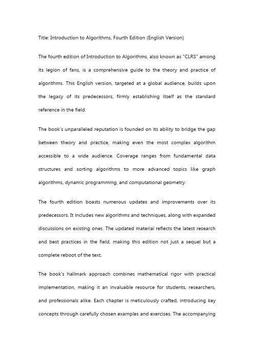
Title: Introduction to Algorithms, Fourth Edition (English Version)The fourth edition of Introduction to Algorithms, also known as "CLRS" among its legion of fans, is a comprehensive guide to the theory and practice of algorithms. This English version, targeted at a global audience, builds upon the legacy of its predecessors, firmly establishing itself as the standard reference in the field.The book's unparalleled reputation is founded on its ability to bridge the gap between theory and practice, making even the most complex algorithm accessible to a wide audience. Coverage ranges from fundamental data structures and sorting algorithms to more advanced topics like graph algorithms, dynamic programming, and computational geometry.The fourth edition boasts numerous updates and improvements over its predecessors. It includes new algorithms and techniques, along with expanded discussions on existing ones. The updated material reflects the latest research and best practices in the field, making this edition not just a sequel but a complete reboot of the text.The book's hallmark approach combines mathematical rigor with practical implementation, making it an invaluable resource for students, researchers, and professionals alike. Each chapter is meticulously crafted, introducing key concepts through carefully chosen examples and exercises. The accompanyingonline resources also provide additional challenges and solutions, further enhancing the learning experience.In conclusion, Introduction to Algorithms, Fourth Edition (English Version) is more than just a textbook; it's a roadmap to understanding the intricacies of algorithms. Its comprehensive nature and timeless quality make it a must-have for anyone serious about mastering the art and science of algorithm design.。

C4FresnelandFraunhoferdiffraction

$C4FresnelandFraunhoferdiffraction$

Kirchhoff rather than RayleighSommerfeld analysis remains valid for diffraction between two spherical caps.
Review of physical optics_5
Fraunhofer diffraction
Examples of Fraunhofer diffraction_1
Let the apertures are illuminated by a unit amplitude, normally incident plane wave, then
the light field behind the aperture U(,)= tA(,)
Review of physical optics_3
Convolution form of Fresnel diffraction
hx,
y
ejkz
jz
exp2jkz
x2 y2
Ux, yU,h,
Review of physical optics_4
FT form of Fresnel diffraction
intercept portions of a wavefield that were emitted later in time, the phasor will have advanced in the clockwise direction, and therefore the phase must become more negative
Fresnel Diffraction Between Confocal Spherical Surfaces

spatial behaviour) Data

WIRELESS GESTURE CONTROLLERS TO AFFECT INFORMATIONSONIFICATIONKirstyBeilharzKey Centre of Design Computing and Cognition,Faculty of Architecture,University of Sydney,Sydney,Australia.Kirsty@.auABSTRACTThis paper proposes a framework for gestural interaction with information sonification in order to both monitor data aurally but, in addition, to interact with it, transform and even modify the source data in a two-way communication model (Figure 1). Typical data sonification uses automatically generated computational modelling of information, represented in parameters of auditory display, to convey data in an informative representation. It is essentially a one-way data to display process and interpretation by users is usually a passive experience. In contrast, gesture controllers, spatial interaction, gesture recognition hardware and software, are used by musicians and in augmented reality systems to affect, manipulate and perform with sounds. Numerous installation and artistic works arise from motion-generated audio. The framework developed in this paper aims to conflate those technologies into a single environment in which gestural controllers allow interactive participation with the data that is generating the sonification, making use of the parallel between spatial audio and spatial (gestural) interaction. Converging representation and interaction processes bridge a significant gap in current sonification models. A bi-modal generative sonification and visualisation example from the author’s sensate laboratory illustrates mappings between socio-spatial human activity and display. The sensor cow project, using wireless gesture controllers fixed to a calf, is described to exemplify some of the real time computation and representation issues to convey spatial motion in an easily recognised sonification thatFigure 1. Knowledge flows from socio-spatial activities to sensors that capture data, through a computational process generating a visualisation/sonification in real time. This loop is completed when gestural controllers are used for spatial interaction to manipulate or investigate this data.1.INTRODUCTIONBoth information visualisation and information sonification employ a computational process for scaling data, converting it through an algorithmic process of representation, to produce an outcome that is (passively) received by the user. As the objective is to develop a greater rapport with the information, especially socio-spatial data (how people move, relations in spaces, proximity to objects, clustering, eccentric behaviour, velocity and level of traffic), gestural interaction with the information sonification enhances the ability to transform and manipulate the data by interacting with its representation.This interaction is divided into two categories:1)gestural interaction with abstract, remotely-locateddata (stocks, Internet traffic, building lifecycle data,etc.) in which gestural interaction can transform ormanipulate the data by altering the original data set;2)gestural interaction in a sensate space in which thesonification contributes to our understanding of theactivity within the space and the information iscaptured within the space. In this instance, gesturalinteraction is interactivity that becomes furtherreflected in the auditory display. There is adistinction between capture devices (sensors) takingin information and modes of interaction (gesturecontrollers) communicating back into the system.Because socio-spatial data is directly related to positional or spatial axes, 3D spatialised auditory representation has a direct relation with its source data. This utilises the potential of a 3D interface in 3D physical space. Human gestures and sound operate in three dimensional spaces. Three dimensional interaction without traditional mouse and keyboard interfaces underlie the paradigm of non-tactile, seamlessly integrated, pervasive, immersive computing in which the hardware of computing becomes invisible, developing more intuitive interaction.Gestural computing aims to move away from desk-bound, restrictive computing environments and to move towards computing that is more integral to the building structure and space itself. Our environment becomes more reactive, “smart” and the boundaries between architecture and computing or between working and mobility are blurred. The technologies configured in the sensor-cow project contribute to several technical links in this model.2.SOCIAL CONTEXTS FOR RESPONSIVEENVIRONMENTSExisting sonification often focuses on interpretation of abstract data such as meteorological, stock market trends, Internet traffic. These sonification are removed from the data source: context, place and occasionally time. In contrast, the following examples and the sensor-cow project focus on real time sonification in which the outcome and input are experienced simultaneously and co-locationally. Hence, the sonification is intended to help people understand their social and spatial activity and interaction (with other people and with space).Emergent Energy (Figure 2) is an iterative, reflexive system of interaction in which motion, speed, number of users and position in a space (triggering pressure sensitive floor mats) determine the growth of a visual design drawn with a Lindenmayer (L-system) generative algorithm. The design provides both an informative monitor of social and spatial behaviour and invokes users to interact with their space to influence their artistic surrounds. The design artefact is an embedded history of the movements, interactions and number of people who produced it (Figure 3 & Table 1).Figure 2. L-system generator patch in Max/MSP &Jitter used to create branched visualisations on screen.Different behaviours modify the algorithmic process ofdesign generation. Colour of branches indicates spatiallocation, heaviness of lines corresponds to the numberof room occupants and motion affects the rapidity ofbranching. In the corresponding sonification, the number of people relates to dynamic intensity, positionto timbre (tone colour) and speed to frequency (pitch).Figure 3.The Lindenmayer algorithm producesdifferent colours (RGB values) determined by theposition of users on pressure sensitive mats and levelsof activity affect the branching characteristics. Colourcorresponds to different timbres (tone colours) in thesonification and y-axis position determines the pitch(frequency) produced. The sensate room configuration is explained in figures 4 and 5 which show the grid of pressure sensitive mats installed underneath the carpet and connection via Making Things Teleo modules [1] to Max/MSP + Jitter [2]. The shortcoming of this arrangement is obviously its site specificity, hence subsequent experimentation using wireless (mobile) sensors (gesturecontrollers).Figure 5. The author’s Sensate Lab (2 views) showingthe “invisible” pressure sensitive floor mats embedded underneath the carpet, triggering the visual and auditory sound system and (before carpeting) the gridof pressure mats, networked to the Teleo modules. Enabling buildings with responsive, “understanding” and feedback capabilities facilitates flexibility and accessibility to assist environmental comfort, navigation for the visually impaired, building awareness, gerontechnology (technologies assisting the elderly), and automated and augmented tasks for the physically disabled. Nanotechnologies - embedding minute sensor technologies in furnishings, surfaces and pre-fabricated building materials - facilitate localised sensate regions and unobtrusive (wireless) distributed networks for data collection. Intelligence and learning capabilities also transform household and commercial products that we use within our everyday spaces (air conditioners, washing machines, coffee machines) contributing to the picture of our increasingly responsive environment.3.TOWARDS AESTHETIC AND ENGAGINGAMBIENT DISPLAYScientific sonification or visualisation of abstract data is usually designed for the purpose of illuminating or augmenting our understanding of abstract (non-visual) data. There are contexts in which sonification is more helpful than visualisation: utilising the human auditory capacity for detecting subtle changes and comprehending dense data; and to avoid overload on visual senses, e.g. during surgery, anaesthesiology, and aircraft control. These applications of visualisation and sonification contribute to our understanding of well-known issues, particularly in regard to sonification: “orthogonality [3, 4] (i.e. changes in one variable that may influence the perception of changes in another variable), reaction times inmulti-modal presentation [5], appropriate mapping betweendata and sound features [6], and average user sensibility for subtle musical changes [7].” There is also evidence to suggest that bimodal (visual and auditory) display has synergisticbenefits for information representation [8, 9].Figure 4. Configuration of sensate system indicating input from digital pressure sensor mats (and other sensor devices triggered by user interaction – button, infra-red, piezo pressure detection, temperature, light-sensitive photocells, proximity,RFID tags) that provide data for the generative information representation process.Table 1. Sonification schema of mapping correspondencesSonification Visualisation Activity / TriggerPitch (frequency) Length/scale/scope of graphic display on screen Distance between activities / motionTexture/density Density of events / number of branches or iterations of generative algorithm (embeds history by amount of activity)Volume of activity, number of users and social thresholdRhythm/tempo of events Proximity and rapidity of display (animation) Speed of actions, punctuation of triggering events, tied to velocity of eventsIntensity/dynamic loudness Heaviness and distinction of on-screen drawing Intensity/magnitude of triggering events Timbre (tone colour) Colour and distribution on visual display (screen) Region/spatialisation – topology, zoning HarmonyDesign artefactMulti-user manipulationVisualisation and sonification provide useful infotainment for monitoring and display in public spaces, designed to augment, enhance and contribute artistically (as well as informatively) to our experience of spaces, e.g. a foyer, sensate space, common room. Aesthetic representation and accessibility (comprehensibility) directly influences the perception and reception of a work. Granularity or magnification (preprocessing, scaling and density of mapping) also affects our ability to comprehend the representation [10].Stochastic, algorithmic, generative and deterministic processes applied to musical composition almost always utilise source data predominantly to create “aesthetic” works of art. Rules or grammars of interpretation for transforming algorithmic or non-visual data into auditory parameters are selected to maximise musical effect. Music composers whoemploy such systematic ways of designing include integral serialists and stochastic composers, Karlheiz Stockhausen, Iannis Xenakis and Pierre Boulez [11]. Ambient sonification concerned with raising awareness of socio-spatial trends in building spaces, in order to be sustainable and listenable over a long period of time, requires an aesthetic approach to pitch representation and other parameters.It might be argued that sound is even more integrally tied to space than light: “in a natural state, any generated sound cannot exist outside its context” [12] – space is a parameter of sound design, just as is pitch or timbre. The following examples (Table 2) illustrate the variety of data that can provide informative and engaging sonification to map abstract, non-visual data to auditory display with a range of scientific and artistic motivations.Table 2. Examples of the wide variety of information that can be sonified for variously scientific or artistic purposes.Sonification author & titleSource dataCiardi’s sMAX: A Multi-modal Toolkit for Stock Market Data Sonification sonifies data from stock market environments, in which large numbers of changing variables and temporally complex information must be monitored simultaneouslyJanata and Childs MarketBuzzsonification of real-time financial data, in which “auditory display is more effective and consistent for monitoring the movement of volatile market indices” [13]Andrea Polli’s Atmospherics/Weather Workssonified meteorological data designed for museum installation/exhibition with the additional agenda of displaying narrativeGarth Paine’s PLantAusing a weather station [14] to capture dynamic non-visual data measurements of wind velocity, direction, temperature and UV levels [15] Polyrhythm in the Human Brainderived from EEG brain data4. AMBIENT DISPLAY AND AMBIENT DEVICES Ambient visualisation and sonification in buildings merges informative information display with entertainment (infotainment or informative art) bringing a new versatility andpublic spaces. This is where the established practice of installation art works concurs with domestic infotainment.Ambient display devices include plasma, projection, touch screens and audio amplification systems. These output devices can be used for monitoring environmental characteristics – socio-spatial activities. Ambient information representation orpre-attentive display is intentionally peripheral and may doubly serve a role as décor. “Ambient displays normally communicateon the periphery of human perception, requiring minimal attention and cognitive load” [16]. As perceptual bandwidth is minimised, users get the gist of the state of the data source through a quick glance, aural refocus, or gestalt background ambience.In relation to architecture, ambient representation that responds to the building (lighting, airflow, human traffic) as well as to social elements such as human clustering (flocking) patterns, divergences and task-specific data, adds a dimensionof responsiveness to the spatial habitat.ING GESTURAL CONTROLLERS AND SPATIALINTERACTION TO ENGAGE WITH DATA Introducing gestural controllers as a mechanism for interactingwith the 3D spatial auditory and visual representation of information takes this process one step further. There is a chain from building/computer – information – visualisation/sonification – human interaction/manipulation in which tactile, gestural and haptic interfaces provide ways to access and manipulate data and displays without the encumbrance of traditional keyboard/mouse interfaces. The barrier between humans and information, between humans andthe smart building are disintegrated while computation and sensing are conflated into a single organism: the intelligent building.The science fiction film, Steven Spielberg’s Minority Report [17] forecasted a kind of interface that is already now achievable: spatial and gestural manipulation of video and computer data on a transparent screen suspended in 3D space (Figure 6). The notion behind gestural information access is an important one: dissolving the hardware and unsightliness of computer interfaces. As computing moves towards people acting in spaces, deviating from our currently sedentary desk-bound lifestyle, the importance of the spatial interaction and experience design, the way in which information is represented, becomes essential. Building architecture and information architecture become one (Figures 1, 7 & 8).Figure 6. Justin Manor’s Manipulable CinematicLandscapes [17] is a glove-controlled cinematiclandscape interface in 3D space.Figure 7. Haptic (tactile) manipulable cubes in ReedKram’s Three Dimensions to Three Dimensions (top)are creative tools for expression while sensors attachedto digits and limbs can be used as gestural controllersfor music (bottom) [12, 18, 19].Figure 8.A gestural Cyberglove controller thatproduces a high degree of accuracy transmittingspatial, position, rotational, gyroscopic, velocity andflex data. The precision facilitates interaction withinformation representation in 3D space [20].5.1.Wireless UDP gesture sensorsIn the Sensor-Cow project (Figure 9), the La Kitchen Kroonde Gamma receiver, transmitter and sensor equipment was used (Figure 10). The Kroonde is a wireless sensor interface dedicated to real time applications. Sensors are connected to the wireless transmitter box (worn by the user) which has an effective 914Mhz wireless range of between 100-300 feet, depending on nearby interference (most effective outdoors). The wireless base transmits this information through a high bandwidth Ethernet connection to the host computer with high precision. The Kroonde can also send the data via MIDI. The range of sensors available includes acceleration, gyroscope, motion, pressure, temperature and photosensitivity.Figure 9.Sensor-Cow: bi-directional (mercury) motion sensors are attached to the calf’s front legs, a gyroscopic sensor on the forehead and accelerometeron his right ear. The pouch hanging around his neckcontains the radio frequency transmitter that sends thereal time data to the (La Kitchen) Kroonde Gammawireless UDP receiver [21]. It is connected by Ethernet to the computer running the data sonification withMax/MSP object-oriented programming environment.Figure 10. Kroonde Gamma wireless receiver box,transmitter and attached sensors. The sensors, cabledto the transmitter box, are worn by the user who is thenfree to move.Figure 11 shows the acceleration sensor (at approximately life-size) used for capturing motion data and the UDP transmitter box. Figure 9 shows the way in which these sensors and transmitter are attached to the calf for capturing the datathat generates the sonification.Figure 11.Acceleration sensor and transmitter box.The highly sensitive mercury motion sensors operate between extremes of direction, registering a “bang” (signal to the sonification program) when changes in direction occur. Thus these were attached to the front legs to indicate steps as the calf walks. When calibrated, the gyroscopic and accelerator sensors produce a broad spectrum of values spanning a gamut of 1024 increments mapped to audible pitches. The acceleration sensor values were scaled to 128 distinct output values. These sensors were attached to the calf’s ear and forehead, respectively, because these regions isolate significant independent gestures. The calf naturally raises and lowers its head to eat, when flicking away flies, in response to people and other animals - it is expressive and the range of motion is diverse. While naturally following whole head movements, the ear is also flicked and rotated independently producing a recognisable gesture (or musical event).5.2.Sonification (mapping) & real-time computationA distinctive timbre (tone colour) is attributed to each sensor in order to make it possible to distinguish the sounds arising from each sensor. The rhythm, pace/acceleration and velocity of action is directly realised in real time. The correspondence between rapid gestures and rapid sonification is literal. For both the acceleration and gyroscopic sensor, extremes of motion away from the median, drives the pitch in directional extremes away from a central pitch region. The direction of pitch, ascending and descending away from the mean, corresponds to the x-axis direction of motion so that changes in direction are audible and circular motions of the ear and head produce sweeping auditory gestures that reinforce the audio-visual connection between activity and sonification. The Max/MSP (+Jitter) patch (Figure 12) shows the input reading on the sliders at the top using La Kitchen’s Kroonde Gamma patch [22] corresponding to the 4 active sensors, 8 active transmitter channels and potential 16 channel capability of the Kroonde device. The relevant channels are coloured in the diagram, the sonification effects corresponding in colour to the slider input. This Max patch receives the data via Ethernet connection at a fixed IP address. The hardware is recognised using CNMAT Berkeley’s Open Sound Control [23] object. Channels 2-4 (gyroscope and mercury motion sensors) each have an inbuilt threshold within which no sound is produced. Thus stasis produces no constant throughput on these channels. In contrast, channel 1, the acceleration sensor, sonifies a constant data stream, including when the calf is still.Figure 12.Max/MSP patch. Data is received wirelessly by the Kroonde Gamma and communicated to the computer by Ethernet. Information is received from its fixed IP address at the top left of the program. The sliders provide a visual monitor of the input signal (the first four channels are active in this project, corresponding to the four sensors) linked to its processing, correspondingly coloured. The information from the first (acceleration) sensor is scaled or calibrated from 1024 increments to 128 output values. An alternative output process for this channel is included but not linked in this example. Channels 2 (gyroscope), 3 and 4 (mercury motion sensors) share a similar sonification process in which superfluous throughput is discarded to reduce the number of pitches heard. Consecutive (repeated) pitches are eliminated and for channels 2, 3 and 4 there is threshold of inactivity that is not sonified so that only more significant gestures are heard. These limitations are imposed to simplify the sonification and facilitate auditory comprehension. Each channel has a distinctive tone colour whichcan be changed for different effect.Real-time computation presents several challenges for a modest, portable system because the constant stream of data from the sensors generates massive continuous throughput in the algorithm-to-MIDI chain. When employing a complex elaborative generative system, such as the Lindenmayer evolutionary tree growth triggered by activity on sensor mats (Figures 2 & 3), the system quickly acquires a vast amount of information, at risk of crashing and of saturating the listener. To avoid overloading the output (from a human listener’s perspective) and to avoid stifling the algorithmic generative process, the L-system model limited the periodicity of input capture and restricted the pitch continuity of auditory output.In the sensor-cow project, the computation is less complex and, in order to make the output both less consuming for the processor and less complex to audit, the broad bandwidth of pitch output was calibrated, scaled and limited to produce pitches separated by small increments rather than producing every available pitch. Gestural motion is still very evident and the result is sufficiently rich to not eliminate any vital data. The sensor-cow patch only uses Max/MSP (the sound processing objects) to produce sonification but if a bi-modal sonification and visualisation is developed using Jitter (processing video objects), a further reduced auditory output would enable faster processing within current equipment limitations.5.3.Monitoring spatial activityWhile the sensor-cow project acts as a monitor of calf motion, and it is unlikely that the calf understands the affects of its actions in contributing to the sonification, socio-spatially generated sonification has the potential in a human context to invoke interaction with the outcome. In a building, people become aware that social group behaviour and different levels of activity influence their experience of the environment. Socio-spatial monitors can tell us about the clustering behaviour of people, trends in motion - paths of flow in a building, peak times of activity, popular junctions and patterns of behaviour related to tasks.In summary, this paper outlines some ways in which sensate environments and wireless sensors can capture three dimensional spatial and social (behavioural) data to realise a representation of patterns, cliques, clusters and eccentricities inreal time responsive environments. Designing the responsive experience with increasingly accessible pre-fabricated sensors and retro-fitted sensate technologies allows building design to flow into the realm of experience and interaction design, dissolving barriers between the computation machine and the visualisation/sonification space. Gestural controllers provide a mechanism for spatial interaction with data representation that absolves the need for visible computing interfaces such as the mouse, keyboard and conventional monitors. Seamless integration of spatial experience and computational response is a direction essential to the future of designing spaces.The gestural controllers used to activate the sonification of movements in the sensor-cow project provide a working model to pilot test the fine incremental detail transmitted by wireless sensors. The pilot project trials recognisable sonification mapping to represent gestural activity and explores some practical issues associated with spatial freedom, mobility, processing and deciphering signals from a group of distinctive sensors transmitting information about a single individual’s behaviour.6.GESTURE AFFECTED COMPUTATION:COMPLETING THE INTERACTION LOOP Finally, translating gestural interaction in 3D space into affectors (software commands) that manipulate the source data demonstrates a complete cycle in which social activities and movement throughout a room produces the sonification that, in turn, can be transformed by the participant. The notion that spatial gesture can affect the source information is applicable in other situations in which the data is abstract and non-social (i.e. not reflexive, iterative) and removed from the context of data capture. Affectors, in programming terms, are gestures that trigger a change in information, e.g. motion acceleration thresholds, direction, velocity. The specific affectors are determined by the nature of data sonified and the type of sensors/controllers used. The relations between gestures and affects (transformations) are determined by the sonification designer, in the mapping process. Spatialised audio display (e.g. using IRCAM’s multi-channel SPAT) locates sound attributes in 3D space, making it easier to identify, distinguish, then manipulate specific sounds. As sound represents data through the mapping process, moving the sound or interacting with it gesturally is essentially a reverse-mapping procedure that alters the data set. Successful gestural interaction with data sonification can be demonstrated by using gesture controllers to change the data set producing the sonification experienced by the participant (Figure 13). Figure 13. Gestural interaction using gesture controller devices can be used to affect (change) the source data that produces the information sonification in real time. In the situation described in this paper, the sourceinformation derives from socio-spatial data about human behaviour in a sensate architectural space. The underlying principle of interactive informationsonification can be applied to other contexts.7.REFERENCES[1] (2003) MakingThings Teleo Modules and Sensor Devices/products/products.htm1/1/04.[2] IRCAM (2003).Max/MSP, Cycling 74: Max/MSP is agraphical environment for music, audio, and multimediaobjects-oriented control, USA./products/maxmsp.html[3] Ciardi, F.C. sMAX: A Multimodal Toolkit for Stock MarketData Sonification. in Proceedings of ICAD 04 -TenthMeeting of the International Conference on AuditoryDisplay. 2004. Sydney, Australia.[4] Neuhoff, J.G., G. Kramer, and J. Wayand. Sonification andthe Interaction of Perceptual Dimensions: Can the DataGet Lost in the Map? in International Conference onAuditory Display. 2000. Atlanta, Georgia, USA.[5] Nesbitt, K.V. and S. Barrass. Evaluation of a MultimodalSonification and Visualisation of Depth of Market StockData. in International Conference on Auditory Display(ICAD). 2002. Kyoto, Japan.[6] Walker, B.N. and G. Kramer. Mappings and Metaphors inAuditory Displays: An Experimental Assessment. inInternational Conference on Auditory Display (ICAD).1996. Palo Alto, California, USA.[7] Vickers, P. and J.L. Alty. Towards some OrganisingPrinciples for Musical Program Auralisations. inInternational Conference on Auditory Display (ICAD).1998. Glasgow, Scotland, U.K.[8] Song, H.J. and K. Beilharz. Time-based Sonification forInformation Representation. in World Multi-Conference on Systemics, Cybernetics and Informatics. 2005. Orlando,USA.[9] Song, H.J. and K. Beilharz. Some Strategies for ClearAuditory Differentiation in Information Sonification. inKCDC Working Paper. 2004. University of Sydney. [10] Beilharz, K. (Criteria & Aesthetics for) Mapping SocialBehaviour to Real Time Generative Structures for Ambient Auditory Display (Interactive Sonification). inINTERACTION - Systems, Practice and Theory: ACreativity & Cognition Symposium. 2004. The DynamicDesign Research Group, UTS, Sydney: Creativity andCognition Press.[11] Beilharz, K., Designing Sounds and Spaces:Interdisciplinary Rules & Proportions in GenerativeStochastic Music and Architecture. Journal of DesignResearch, 2004: p. in press.[12] Pottier, L. and O. Stalla. Interpretation and Space. inTrends in Gestural Control of Music. 2000. Paris: IRCAM - Centre Pompidou.[13] Janata, P. and E. Childs. Marketbuzz: Sonification of Real-Time Financial Data. in International Conference ofAuditory Display (ICAD). 2004. Sydney, Australia. [14] Paine, G. Reeds: A Responsive Sound installation. inInternational Conference of Auditory Display (ICAD).2004. Sydney, Australia.[15] Hermann, T., G. Baier, and M. Müller. Polyrhythm in theHuman Brain. in International Conference of AuditoryDisplay (ICAD). 2004. Sydney, Australia.[16] (2004) ADG Berkeley Ambient Display Group/projects/io/ambient/[17] Maeda, J., Creative Code. 2004, London: Thames andHudson. [18] Choi, I. Gestural Primitives and the Context forComputational Processing in an Interactive Performance System. in Trends in Gestural Control of Music. 2000.Paris: IRCAM - Centre Pompidou.[19] Rovan, J. and V. Hayward. Typology of Tactile Soundsand their Synthesis in Gesture-Driven Computer MusicPerformance. in Trends in Gestural Control of Music.2000. Paris: IRCAM - Centre Pompidou.[20] Bongers, B. Physical Interfaces in the Electronic Arts.Interaction Theory and Interfacing Techniques for Real-timePerformance. in Trends in Gestural Control of Music.2000. Paris: IRCAM - Centre Pompidou.[21] (2004) LaKitchen Kroonde Gamma 16-sensor WirelessUDP Interface/products/kroonde.html03/08/04.[22] Henry, C., La Kitchen Kroonde Gamma - User Manual &Max Patches. 2004, Paris: La Kitchen.[23] (2004) CNMAT Open Sound Control (OSC)/OSC/Max/#downloads。

毕设英译汉原文协作数据共享系统的可靠存储和查询

Reliable Storage and Querying for CollaborativeData Sharing SystemsNicholas E.Taylor and Zachary G.IvesComputer and Information Science Department,University of PennsylvaniaPhiladelphia,PA,U.S.A.{netaylor,zives}@Abstract—The sciences,business confederations,and medicine urgently need infrastructure for sharing data and updates among collaborators’constantly changing,heterogeneous databases.The O RCHESTRA system addresses these needs by providing data transformation and exchange capabilities across DBMSs,com-bined with archived storage of all database versions.O RCHESTRA adopts a peer-to-peer architecture in which individual collabo-rators contribute data and compute resources,but where there may be no dedicated server or compute cluster.We study how to take the combined resources of O RCHES-TRA’s autonomous nodes,as well as PCs from“cloud”services such as Amazon EC2,and provide reliable,cooperative storage and query processing capabilities.We guarantee reliability and correctness as in distributed or cloud DBMSs,while also sup-porting cross-domain deployments,replication,and transparent failover,as provided by peer-to-peer systems.Our storage and query subsystem supports dozens to hundreds of nodes across different domains,possibly including nodes on cloud services.Our contributions include(1)a modiﬁed data partitioning substrate that combines cluster and peer-to-peer techniques, (2)an efﬁcient implementation of replicated,reliable,versioned storage of relational data,(3)new query processing and indexing techniques over this storage layer,and(4)a mechanism for incre-mentally recomputing query results that ensures correct,com-plete,and duplicate-free results in the event of node failure during query execution.We experimentally validate query processing performance,failure detection methods,and the performance beneﬁts of incremental recovery in a prototype implementation.I.I NTRODUCTIONThere is a pressing need today in the sciences,medicine, and even business for tools that enable autonomous parties to collaboratively share and edit data,such as information on the genome and its functions,patient records,or component designs shared across multiple teams.Such collaborations are often characterized by diversity across groups,resulting in different data representations and even different beliefs about some data(such as competing hypotheses or diagnoses from the same observations).Data is added and annotated by dif-ferent participants,and occasionally existing items are revised or corrected;all such changes may need to be propagated to others.To maintain a record across changes,different versions of the data may need to be archived.In these collaborative settings,there is often no single authority,nor global IT group, to manage the infrastructure.Hence,it may be economically or politically infeasible to create centralized services in support of data transformation,change propagation,and archival.To address these needs,we have been developing the O RCHESTRA collaborative data sharing system(CDSS)[1].Brieﬂy,O RCHESTRA adopts a peer-to-peer architecture for data sharing,where each individual participant owns a local DBMS with its own preferred schema,makes updates over this DBMS,and periodically publishes updates to others.Then the participant translates others’published updates to its own schema via schema mappings and imports them.O RCHESTRA especially targets scientiﬁc data sharing applications such as those in the life sciences,where data sets are typically in the GB to10s of GB,and changes are published periodically and primarily consist of new data insertions.Previous work on O RCHESTRA has developed the upper layers of our system architecture:strategies and algorithms for resolving conﬂicts[2],and for generating the necessary queries to propagate data and updates across sites or peers[3]. Such work temporarily used a centralized DBMS to handle storage and query processing.In this paper,we complete the picture,with a highly scalable and reliable versioned storage and query processing system for O RCHESTRA,which does not require dedicated server machines.Rather,we employ the existing CDSS nodes,possibly in combination with machines leased as-needed from cloud services such as Amazon EC2. Our goal is to provide the beneﬁts of peer-to-peer ar-chitectures[4],[5],[6],[7],[8](such as support for au-tonomous domains with no commonﬁlesystem,transparent handling of membership changes,and plug-and-play opera-tion),hybridized with the beneﬁts commonly associated with traditional parallel DBMSs and with emerging cloud data management platforms[9],[10],[11],[12](such as efﬁcient data partitioning,automatic failover and partial recomputation, and guarantees of complete answers).We avoid what we perceive to be the negative aspects of each architecture:the lack of completeness or consistency guarantees in peer-to-peer query systems,and requirements for sharedﬁlesystems and centralized administration in the existing cloud data manage-ment services(e.g.Google’s GFS[9],Amazon’s S3[12]). To accomplish this,we exploit the fact that our system does not need all of the properties provided by existing distributed substrates.Our problem space is less prone to “churn”than a traditional peer-to-peer system like a distributed hash table:we assume that membership in a CDSS,while not completely stable,consists of perhaps dozens to hundreds of participants at academic institutions or corporations,with good bandwidth and relatively stable machines.We support archived storage of data under a batch-oriented update load:Participantwith local DB servers + storageAll participantsFig.1.Basic architectural components in the O RCHESTRA system,as a participant(peer)publishes its update logs and imports data from elsewhere. Components on the left were the focus of[2],[3],and this paper focuses on the components shown on the right.in a CDSS,usersﬁrst make updates only to their local storage, and they occasionally publish a log of these updates(which are primarily insertions of new data items)to the CDSS.Then they perform an import(transforming and importing others’newly published data to their local replica).Only in this step is information actually shared across users,and it is then that conﬂict resolution is performed.Hence,we do not need special support for global consistency,such as distributed locking or version vectors,at the distributed storage level. We address these needs through a custom data partitioning and storage layer,as well as a new distributed query processor. We develop novel techniques for ensuring versioning,con-sistency,and failure recovery in order to guarantee complete answers.Our speciﬁc contributions are as follows:•Modiﬁcations to the standard data partitioning tech-niques used in distributed hash tables[4],customizing them to a more stable environment,and providing greater transparency of operation to the layers above.•A distributed,replicated,versioned relational storage scheme that ensures that queries see a consistent,com-plete snapshot of the data.•Mechanisms for detecting node failures and either com-pletely restarting or incrementally recomputing the query, while ensuring the correct answer set is returned.•Experiments,using standard benchmarks for OLAP and schema mapping tasks,across local and cloud computing nodes,validating our methods under different network settings and in the presence of failures.We implement and evaluate our techniques within the O RCHESTRA collaborative data sharing system.However,the techniques are broadly applicable across a variety of emerging data management applications,such as distributed version control,data exchange,and data warehousing.Section II presents the O RCHESTRA architecture,and Sec-tion III details our modiﬁed data distribution substrate.Sec-tion IV describes our storage and indexing layer,upon which we build the fault-tolerant distributed query engine presented in Section V.Section VI validates our techniques through ex-perimental analysis.We describe related work in Section VII, and conclude and discuss future work in Section VIII.II.S YSTEM A RCHITECTURE AND R EQUIREMENTS Figure1shows O RCHESTRA’s architecture,and sketches the dataﬂow involved in its main operations.Each participant (illustrated on the left)operates a local DBMS with a possibly unique schema,and uses this DBMS to pose queries and make updates.O RCHESTRA is invoked when the participant has a stable data instance it wishes to“synchronize”with the world: this involves publishing updates from the local DBMS log to versioned storage,and importing updates from elsewhere. The import operation consists of update exchange[3]and reconciliation[2].Update exchangeﬁnds updates satisfying a local participant’sﬁltering criteria and,based on the schema mappings,executes SQL queries that convert data into the par-ticipant’s local schema.Reconciliationﬁnds sets of conﬂicts, among both updates and the transactions they comprise,by executing SQL queries over the versioned storage system. To this point,our work has focused on the left half of theﬁgure:the logic needed to create and use the SQL queries supporting update exchange and reconciliation,and the modules to“hook”into the DBMS to obtain update logs. In this paper,we focus on the right half of the diagram:how to implement distributed,versioned storage and distributed query execution.We are particularly concerned with performance in support of update exchange(data transformation)queries, which are more complex than the conﬂict detection queries, and by far the main bottleneck in performance[2],[3].We also develop capabilities in the query execution layer to support mapping and OLAP-style queries directly over the distributed, versioned data.Data is primarily stored and replicated among the various participants’nodes.However,as greater resources, particularly in terms of CPU,are required,participants may purchase cycles on a cloud computing service capable of running arbitrary code,such as Amazon’s EC2(considered in this paper)or Microsoft’s Azure.In the remainder of this section,we explain the unique requirements of O RCHESTRA and why they require new solutions beyond the existing state of the art.In subsequent sections,we describe our actual solutions.A.Data Storage,Partitioning,and Distributed LookupAs discussed previously,we assume that the participants number in the dozens to hundreds,are usually connected, and have enough storage capacity to maintain a log of all data versions.Our target domain differs from conventional P2P systems where connectivity is highly unstable.We only expect low“churn”(nodes joining and leaving the system) rates,perhaps as participants go down for maintenance or are replaced with new machines.We expect failures to be infrequent enough that keeping a few replicas of every data item is sufﬁcient.We avoid single points of failure,as we want the service to remain available at all times,even if some nodes go down for maintenance.In a distributed implementation of a CDSS,we need a means of(1)partitioning the stored data(such that it is distributed reasonably uniformly across the nodes),(2)ensuring efﬁcient re-partitioning when nodes join and leave,(3)supporting distributed query computation,and(4)supporting background replication.There are two main schemes for doing this in a distributed system:distributing data page-by-page in a distributedﬁlesystem,and then using a sort-or hash-basedscheme to combine and process the data;and distributing data tuple-by-tuple according to a key,and using a distributed hash scheme to route messages to nodes in a network.Google’s MapReduce and GFS,as well as Hadoop and HDFS,use the former model.Distributed hash tables(DHTs)[4],[7],[8]and directory-based schemes use the latter.Distributedﬁlesystems suffer from several drawbacks as the basis of a query engine.First,they require a single administrative domain and(at least in current implementations like HDFS)a single coordinator node(the NameNode),which introduces a single point of failure.Moreover,they actually use two different distribution models:base data is partitioned on a per-page basis,then all multi-pass query operations(joins, aggregation,nesting)must be executed through a MapReduce scheme that partitions the data on keys(via sorting or hashing). We instead adopt a tuple-by-tuple hash-based distribution scheme for routing messages:this is commonly referred to as a content addressable overlay network and is exempliﬁed by the DHT.Our goal is to provide good performance and to tolerate nodes joining or failing,but we do not require scalability to millions of nodes as with the DHT.In Section III we adapt some of the key ideas of the DHT in order to accomplish this.B.Versioned StorageEach time a participant in O RCHESTRA publishes its up-dates,we create a new version of that participant’s update log(stored as tables).This also results in a new version of the global state published to the CDSS.Now,when a participant in O RCHESTRA imports data via update exchange and reconciliation,it expects to receive a consistent,complete set of answers according to some version of that global state.We support this with a storage scheme(described in Section IV)that tracks state across versions,and manages replication and failover when node membership changes,such that queries receive a“snapshot”of the data according to a version.We optimize for the fact that most published updates will be new data rather than revisions to current data. When data is stored in a traditional content-addressable network,background replication methods ensure that all data eventually is replicated,and gets placed where it belongs when a node fails—but if the set of participants is changing then data may temporarily be missed during query processing.Fur-thermore,such systems also require the data assigned to each key to be immutable.Similarly,existing distributedﬁlesystems like GFS and HDFS assume data is within immutableﬁles, and they are additionally restricted to a single administrative domain.Hence our versioned storage scheme must provide book-keeping than a traditional distributed hash table,but offers more autonomy andﬂexibility than a distributedﬁlesystem. In Section III we describe our customized data storage,parti-tioning,and distributed lookup layer.C.Query Processing LayerAs is further discussed in Section VII,a number of exist-ing query processing systems,including PIER[5]and Sea-weed[6],have employed DHTs to perform large-scale,“best-effort”query processing of streaming data.In essence,the(a)Pastry-style rangeallocation(b)Balanced range allocationFig.2.Range allocation schemesDHT is treated like a very large parallel DBMS,where hashing is used as the basis of intra-operator parallelism.Immutable data can be stored at every peer,accessed by hashing its index key.Operations like joins can be performed by hashing both relations according to their join key,co-locating the relations to be joined at the same node.Such work has two shortcomings for our context:multiple data versions are not supported,and their“best-effort”consistency model in the presence of failures or node membership changes is insufﬁcient.Our goal is not only to support efﬁcient distributed compu-tation of query answers,but also to detect and recover from node failure.We emphasize that this is different from recovery in a transactional sense:here our goal is to compensate for missing answers in a query,ideally without redoing the entire query from scratch(whereas transactional recovery typically does involve aborting and recomputing from the beginning). Failure recovery in query answering requires us(in Section V) to develop techniques to track the processing of query state, all the way from the initial versioned index and storage layer, through the various query operators,to theﬁnal output. Furthermore,we develop techniques for incrementally re-computing only those results that a failed node was responsible for producing.Given that every operator in the query plan may be executed in parallel across all nodes,the failure of a single node affects intermediate state at all levels of the plan.Our goal is to restart the query only over the affected portions of the data,and yet to ensure that the query does not produce duplicate or incorrect answers.III.H ASHING-B ASED S UBSTRATEAny scalable substrate for data storage in a peer-to-peer setting needs to adopt techniques for(1)data partitioning, (2)data retrieval,and(3)handling node membership changes, including failures.We describe how our custom hashing-based storage layer addresses these issues,in a way that is fully decentralized and supports multiple administrative domains.A.Data PartitioningLike most content-addressable overlay networks,we adopt a hash-based system for data placement.Similar to previous well-known distributed hash tables(DHTs)such as Pastry[4], we use as our key space160-bit unsigned integers,matching the output of the SHA-1cryptographic hash function.It is convenient to visualize the key space as a ring of values, starting at0and increase clockwise until they get to(2160−1) and then overﬂow back to0.Figure2shows two examples of this ring that we will discuss in more detail.Most overlay networks assign a position in the ring to each node according to a SHA-1hash of the node’s IP address (forming a DHT ID).Values are placed at nodes according to the relationship with their hash keys.In Chord,keys are placedat the node whose hashed IP address lies ahead of them on the ring;in Pastry the keys are placed at the node with nearest hash value.The Pastry scheme is visualized in Figure2(a).Both of these approaches can determine the range a node“owns,”given its ID and the IDs of its neighbors.These schemes are optimized for settings with large numbers of nodes,and assume the nodes will be more or less uniformly distributed across the ring.Each node maintains information about the position of a limited number of its neighbors,as it has a routing table with a number of entries logarithmic in the membership of the DHT.When there are only dozens or hundreds of nodes, we often see highly nonuniform distributions of values among the peers.Indeed,in theﬁgure,nodes n3and n4are togetherresponsible for more than34of the key space,while node n2is only responsible for116of it.Our substrate adopts Pastry’s routing approach for large numbers of peers(with an expanded routing table,as discussed later in this section).However,for smaller numbers of peers, we support an alternative solution that provides more uniform data distribution(which we use for the experiments in this paper).We divide the key space into evenly sized sequential ranges,one for each node,and assign the ranges in order to the nodes,sorted by their hash ID.Such an assignment for the same network we examined for Pastry-style routing is shown in Figure2(b);it distributes the key space,and therefore the data,uniformly among the nodes.In principle, we could also use many virtual nodes at each physical node to better distribute the key space.However,it is advantageous to assign a single contiguous key range to each node;in addition to reducing the size of the routing table,this improves data retrieval performance,as discussed in Section IV.In response to node arrival or failure,we redistribute the ranges over the new node set.We consider the implications of this when we describe node arrival and departure later in this section.B.Data RetrievalAs mentioned above,a traditional DHT node maintains a routing table with only a limited number of entries(typically logarithmic in the number of nodes).This reduces the amount of state required,enabling greater scale-up,but requires mul-tiple hops to route data.Recent peer-to-peer research has shown[13]that storing a complete routing table(describing all other nodes)at each node provides superior performance for up to thousands of nodes,since it provides single-hop communication in exchange for a small amount of state;we therefore adopt this approach.Our system requires a reliable, message-based networking layer connection withﬂow control. We found experimentally that,for scaling at least to one hundred nodes,maintaining a direct TCP connection to each node was feasible.With the use of modern non-blocking I/O, a single thread easily supports hundreds or thousands of open connections.For larger networks,a UDP-based approach could be developed to avoid the overhead of maintaining TCP’s in-order delivery guarantees,as all of the techniques in this paper are independent of message ordering.C.Node Arrival and DepartureTraditional DHTs deal with node arrival and departure through background replication.Each data item is replicated at some number of nodes(known as the replication factor). In Pastry,for example,for a replication factor r,each item is replicated atr2nodes clockwise from the node that owns it, and the same number counterclockwise from it,leading to r total copies.In the ring of Figure2(a),if r=3,each data item that is owned by node n1will be replicated to n4and n2as well.When a node joins,background replication slowly brings all data items that a node owns to it,as they must be stored at one of its neighbors.If a node leaves,each of its neighbors already has a copy of the data that it owned,so they are ready to respond to queries for data stored at the departed node. This approach makes an implicit assumption that all of the state at the nodes is stored in the DHT,and therefore that any node that has a copy of a particular data item can handle requests for it.If a node joins or fails,certain requests will suddenly be re-routed to different nodes,which are assumed to provide identical behavior(and hence do not get notiﬁed of this change).This does not work in the case of a distributed query processor,where in addition to persistent stored data there may be distributed“soft state”that is local to a query and is not replicated;this includes operator state,such as the intermediate results stored in a join operator or an aggregator. If data for a particular range is suddenly rerouted from one node to another,tuples might never“meet up”with other tuples they should join with,or data for a single aggregate group may be split across multiple nodes,causing incorrect results.To solve this problem,our system works on snapshots of the routing table.When a participant initiates a distributed computation,it sends out a snapshot of its current routing table,which all nodes will use in processing this request. Therefore,if a new node joins in mid-execution,it does not participate in the current computation(otherwise it may be missing important state from messages prior to its arrival).If a node fails,the query processor can detect what data was owned by the failed node,and thus can reprocess this state (this is discussed in Section V-D).Our system must still handle replication of base data, which is done in a manner very similar to that of Pastry; each data point is replicated atr2nodes clockwise and counterclockwise from the node that owns it.This ensures that data can survive multiple node failures,and that in the event of a node failure,the nodes that take over for a failed node have copies of the base data for the sections of the ring they are newly responsible for.Unlike in Pastry,a single node arrival or departure will cause all the ranges in the range to change slightly;this causes a membership change to be more expensive,but we are assuming reasonable bandwidth and less frequent failures.With smaller numbers of fairly reliable nodes,the performance beneﬁts of uniform distribution likely outweigh the costs of extra shipping.Currently we only replicate data as it is inserted into the DHT.This has been sufﬁcient for the development and experimental analysis of our system,since we inserted databefore any node failures,and failed few enough nodes that data was never lost.For completeness we plan to implement the Bloomﬁlter-based background replication approach of the Pastry-based PAST storage system[14],which can be directly applied to our context.IV.V ERSIONED D ATA S TORAGERecall from our earlier discussion that O RCHESTRA sup-ports a batched publish/import cycle,where each participant stores its own updates in the CDSS,disjoint from all others. There is no need for traditional concurrency control mech-anisms,as conﬂicts among concurrent updates are resolved during the import stage(via reconciliation)by the participant. However,there is indeed a notion of global consistency.We assign a logical timestamp(epoch)that advances after each batch of updates is published by a peer.When a participant performs an import or poses a distributed query,it is with respect to the data available at the speciﬁc epoch in which the import starts.The participant should receive the effects of all state published up to that epoch,and no state published thereafter(until its next import).The current epoch can be determined through a simple“gossip”protocol and does not require a single point of failure.Of course,in order to support queries over versioned data, we must develop a storage and access layer capable of managing such data.There are several key challenges here:•Between database versions,we want to efﬁciently reuse storage for data values that have not changed.•We must track which tuples belong to the desired version of a database.Such metadata should be co-located with the data in a way that minimizes the need for communi-cation during query operation.•Each tuple must be uniquely identiﬁable using a tuple identiﬁer that includes its version.Yet,for efﬁciency of computation,we must partition data along a set of key attributes(as with a clustered index).It must be possible to convert from the tuple ID to the tuple key,so thata tuple can be retrieved by its ID;therefore a tuple’shash key must be derived from(possibly a subset of)the attributes in its ID.We maintain all versions of the database in a log-like structure across the participants:instead of replacing a tuple, we simply update our records to include the new version rather than the old version,which remains in storage.Disk space is rarely a constraint today,and the beneﬁts of full versioning, such as support for historical queries,typically outweigh the drawbacks.Each node,therefore,may contain many versions of each tuple.If the set of nodes is inﬂux,nodes may come and go between when a tuple is inserted or updated and when it is used in a query;therefore,a node may not have the correct version of a particular tuple.We assume that background replication is sufﬁcient to ensure that each tuple exists somewhere in the system,but that it may not exist where the standard content-addressable networking scheme canﬁnd it.The key to our approach is a hierarchical structure that maps from a point in time to the collection of tuple IDs present in a relation at thatFig.3.Storage scheme to ensure version consistency and efﬁcient retrieval. Rounded rectangles indicate the key used to contact each node(whose state is indicated with squared rectangles).time.This collection is used during processing to detect which tuples are missing or stale,and must therefore be retrieved from another node in the system.Figure3shows the main data structures used to ensure con-sistency.All data structures are replicated using the underlying network substrate,so failure of any node will cause all of its functionality to be assumed transparently by one or more neighboring nodes.We distribute all tuples are according to a hashing scheme.Relations are divided into versioned pages, each of which represents a partition over the space of possible tuple keys’hash values.Tuples assigned to the same page will be likely be co-located on a single node,or span two nodes in the worst case.As an optimization,we place the index node entry at the same node as the tuples it references, by storing the index page at the middle of the range of tuple keys it encompasses.This is why the network substrate,as discussed in Section III-A,assigns a large,contiguous region in the key space to each node;it means that the vast majority of tuple keys are never sent over the network.If each node is responsible for many smaller ranges,this is no longer the case,and performance suffers.When requesting a given relation at a given epoch,the storage system hashes these values to get the address of a relation coordinator,who has a list of the pages in the relation at that epoch.The system uses this list,which contains the hash ID associated with each page,toﬁnd the index nodes that contain these pages.From the index nodes,the system retrieves the tuple IDs belonging to the relation at the epoch, which are used to retrieve the full versions of all the tuples in the relation from the data storage node.Recall that as the pages are colocated with most of the tuples they reference, typically a single node serves as both the index node and the data storage node for an entire page,reducing network trafﬁc and improving performance.Our scheme is designed to efﬁciently support small changes to tables.Modifying a tuple in a relation requires us to look up the page holding the old version of the tuple using an inverse node,modify that page to include the ID of the new tuple,and write out that modiﬁed page as the new index page for the region of the table surrounding the updated tuple.The entire contents of the new tuple must also be written out to the network.The system then creates a new version record linking to the updated index page,and all of the unaffected pages from the previous version.We were initially inspired byﬁlesystem i-nodes,the CFS ﬁlesystem[15],and log-structuredﬁlesystems,where for ap-。

1、下载文档前请自行甄别文档内容的完整性，平台不提供额外的编辑、内容补充、找答案等附加服务。
2、"仅部分预览"的文档,不可在线预览部分如存在完整性等问题,可反馈申请退款(可完整预览的文档不适用该条件!)。
3、如文档侵犯您的权益，请联系客服反馈,我们会尽快为您处理(人工客服工作时间：9:00-18:30)。

New spatial techniques
Spatial indices, e.g. grids, hierarchical collection of rectangles Provide better computational performance
Common assumptions for SDBMS physical model
Conceptual model: high level abstract description Logical model: description of a concrete realization Physical model: implementation using basic components
Supports filter and refine processing of queries
Spatial operations
OGIS operations, e.g. topological, spatial analysis Many topological operations are approximated by ―Overlap‖ Common spatial queries - listed in next slide
Concepts in a physical data modeonceptual data model - entity, (multi-valued) attributes, relationship, … Logical model - relations, atomic attributes, primary and foreign keys Physical model - secondary storage hardware, file structures, indices, …
Why learn physical data model concepts?
To be able to choose between DBMS brand names
• Some brand names do not have spatial indices!
To be able to use DBMS facilities for performance tuning For example, If a query is running slow,
Relational DBMS has simple values like numbers Sorting, search trees are efficient for numbers These concepts are not natural for Spatial data (e.g. points in a plane)
Chapter4: Spatial Storage and Indexing
4.1 Storage:Disk and Files 4.2 Spatial Indexing 4.3 Trends 4.4 Summary
Learning Objectives
Learning Objectives (LO)
how to efficiently use storage devices how to structure data files how to use auxiliary(辅助的) data-structures about technology trends in physical data model
Physical models :
• Car: engine, transmission, master cylinder（汽缸）, break lines, brake pads, … • Bicycle: chain from pedal to wheels, gears（齿轮）, wire from handle to brake pads（垫）
Focus on concepts not procedures! Mapping Sections to learning objectives
LO2, LO3 LO4 LO5 4.1 4.2 4.3
Physical model in 3 level design?
Recall 3 levels of database design
An interesting fact about physical data model
Physical data model design is a trade-off（平衡） between
Efficiently support a small set of basic operations of a few data types Simplicity of overall system
Scope of discussion
4.1 Storage:Disk and Files 4.2 Spatial Indexing 4.3 Trends 4.4 Summary
Learn basic concepts in physical data model of SDBMS Review related concepts from physical DM of relational DBMS Reusing relational physical data model concepts
Analogy with vehicles
Conceptual model: mechanisms to move, turn, stop, ... Logical models:
• Car: accelerator pedal（踏板）, steering wheel, brake pedal, … • Bicycle: pedal forward to move, turn handle, pull brakes on handle
• one-dimensional, totally ordered
Operations:
• search on one-dimensional totally order data types • insert, delete, ...
Physical data model for SDBMS
Is relational DBMS physical data model suitable for spatial data?
• one may create an index to speed it up
For example, if loading of a large number of tuples takes for ever
• one may drop indices on the table before the inserts • and recreate index after inserts are done!
Spatial data
Dimensionality of space is low, e.g. 2 or 3 Data types: OGIS data types Approximations for extended objects (e.g. linestrings, polygons) • Minimum Orthogonal Bounding Rectangle (MOBR or MBR) • MBR(O) is the smallest axis-parallel rectangle enclosing an object O
Each DBMS physical model
Choose a few physical DM techniques Choice depends chosen sets of operations and data types
Relational DBMS physical model
Data types: numbers, strings, date, currency
What is a physical data model?
What is a physical data model of a database?
Concepts to implement logical data model Using current components, e.g. computer hardware, operating systems In an efficient and fault-tolerant(容错) manner
Common Spatial Queries and Operations
•Physical model provides simpler operations needed by spatial queries!
•Common Queries
•Point query: Find all rectangles containing a given point. •Range query（范围查询）: Find all objects within a query rectangle. •Nearest neighbor: Find the point closest to a query point. •Intersection query: Find all the rectangles intersecting a query rectangle.
LO1: Understand concept of a physical data model
• What is a physical data model? • Why learn about physical data models?
LO2: LO3: LO4: LO5:
Learn Learn Learn Learn