Multi-party finite computations
丘赛计算与应用数学考试大纲

丘赛计算与应⽤数学考试⼤纲原⽂地址:Computational MathematicsInterpolation and approximationPolynomial interpolation and least square approximation; trigonometric interpolation and approximation, fast Fourier transform; approximations by rational functions; splines.Nonlinear equation solversConvergence of iterative methods (bisection, secant method, Newton method, other iterative methods) for both scalar equations and systems; finding rootsof polynomials.Linear systems and eigenvalue problemsDirect solvers (Gauss elimination, LU decomposition, pivoting, operation count, banded matrices, round-off error accumulation); iterative solvers (Jacobi, Gauss-Seidel, successive over-relaxation, conjugate gradient method, multi-grid method, Krylov methods); numerical solutions for eigenvalues and eigenvectorsNumerical solutions of ordinary differential equationsOne step methods (Taylor series method and Runge-Kutta method); stability, accuracy and convergence; absolute stability, long time behavior; multi-stepmethodsNumerical solutions of partial differential equationsFinite difference method; stability, accuracy and convergence, Lax equivalence theorem; finite element method, boundary value problemsReferences:[1] C. de Boor and S.D. Conte, Elementary Numerical Analysis, an algorithmicapproach, McGraw-Hill, 2000.[2] G.H. Golub and C.F. van Loan, Matrix Computations, third edition, JohnsHopkins University Press, 1996.[3] E. Hairer, P. Syvert and G. Wanner, Solving Ordinary Differential Equations, Springer, 1993.[4] B. Gustafsson, H.-O. Kreiss and J. Oliger, Time Dependent Problems and Difference Methods, John Wiley Sons, 1995.[5] G. Strang and G. Fix, An Analysis of the Finite Element Method, second edition, Wellesley-Cambridge Press, 2008.Applied MathematicsODE with constant coefficients; Nonlinear ODE: critical points, phase space& stability analysis; Hamiltonian, gradient, conservative ODE's.Calculus of Variations: Euler-Lagrange Equations; Boundary Conditions, parametric formulation; optimal control and Hamiltonian, Pontryagin maximum principle.First order partial differential equations (PDE) and method of characteristics; Heat, wave, and Laplace's equation; Separation of variables and eigen-function expansions; Stationary phase method; Homogenization method for elliptic and linear hyperbolic PDEs; Homogenization and front propagation of Hamil ton-Jacobi equations; Geometric optics for dispersive wave equations. References:W.D. Boyce and R.C. DiPrima, Elementary Differential Equations, Wiley, 2009 F.Y.M. Wan, Introduction to Calculus of Variations and Its Applications, Cha pman & Hall, 1995G. Whitham, "Linear and Nonlinear Waves", John-Wiley and Sons, 1974.J. Keener, "Principles of Applied Mathematics", Addison-Wesley, 1988.A. Benssousan, P-L Lions, G. Papanicolaou, "Asymptotic Analysis for Periodic Structures", North-Holland Publishing Co, 1978.V. Jikov, S. Kozlov, O. Oleinik, "Homogenization of differential operators and integral functions", Springer, 1994.J. Xin, "An Introduction to Fronts in Random Media", Surveys and Tutorials in Applied Math Sciences, No. 5, Springer, 2009。
ON THE COMPUTATIONAL COMPLEXITY OF ALGORITHMS
ON THE COMPUTATIONALCOMPLEXITY OF ALGORITHMSBYJ. HARTMANIS AND R. E. STEARNSI. Introduction. In his celebrated paper [1], A. M. Turing investigated the computability of sequences (functions) by mechanical procedures and showed that the setofsequencescanbe partitioned into computable and noncomputable sequences. One finds, however, that some computable sequences are very easy to compute whereas other computable sequences seem to have an inherent complexity that makes them difficult to compute. In this paper, we investigate a scheme of classifying sequences according to how hard they are to compute. This scheme puts a rich structure on the computable sequences and a variety of theorems are established. Furthermore, this scheme can be generalized to classify numbers, functions, or recognition problems according to their compu-tational complexity.The computational complexity of a sequence is to be measured by how fast a multitape Turing machine can print out the terms of the sequence. This particular abstract model of a computing device is chosen because much of the work in this area is stimulated by the rapidly growing importance of computation through the use of digital computers, and all digital computers in a slightly idealized form belong to the class of multitape Turing machines. More specifically, if Tin) is a computable, monotone increasing function of positive integers into positive integers and if a is a (binary) sequence, then we say that a is in complexity class ST or that a is T-computable if and only if there is a multitape Turing machine 3~ such that 3~ computes the nth term of a. within Tin) operations. Each set ST is recursively enumerable and so no class ST contains all computable sequences. On the other hand, every computable a is contained in some com-plexity class ST. Thus a hierarchy of complexity classes is assured. Furthermore, the classes are independent of time scale or of the speed of the components from which the machines could be built, as there is a "speed-up" theorem which states that ST = SkT f or positive numbers k.As corollaries to the speed-up theorem, there are several limit conditions which establish containment between two complexity classes. This is contrasted later with the theorem which gives a limit condition for noncontainment. One form of this result states that if (with minor restrictions)Received by the editors April 2, 1963 and, in revised form, August 30, 1963.285286J. HARTMANIS AND R. E. STEARNS[May»*«, U(n)then S,; properly contains ST. The intersection of two classes is again a class. The general containment problem, however, is recursively unsolvable.One section is devoted to an investigation as to how a change in the abstract machine model might affect the complexity classes. Some of these are related by a "square law," including the one-tape-multitape relationship: that is if a is T-computable by a multitape Turing machine, then it is T2-computable by a single tape Turing machine. It is gratifying, however, that some of the more obvious variations do not change the classes.The complexity of rational, algebraic, and transcendental numbers is studied in another section. There seems to be a good agreement with our intuitive notions, but there are several questions still to be settled.There is a section in which generalizations to recognition problems and functions are discussed. This section also provides the first explicit "impossibility" proof, by describing a language whose "words" cannot be recognized in real-time [T(n) = n] .The final section is devoted to open questions and problem areas. It is our conviction that numbers and functions have an intrinsic computational nature according to which they can be classified, as shown in this paper, and that there is a good opportunity here for further research.For background information about Turing machines, computability and related topics, the reader should consult [2]. "Real-time" computations (i.e., T(n) = n) were first defined and studied in [3]. Other ways of classifying the complexity of a computation have been studied in [4] and [5], where the complexity is defined in terms of the amount of tape used.II. Time limited computations. In this section, we define our version of a multitape Turing machine, define our complexity classes with respect to this type of machine, and then work out some fundamental properties of these classes.First, we give an English description of our machine (Figure 1) since one must have a firm picture of the device in order to follow our paper. We imagine a computing device that has a finite automaton as a control unit. Attached to this control unit is a fixed number of tapes which are linear, unbounded at both ends, and ruled into an infinite sequence of squares. The control unit has one reading head assigned to each tape, and each head rests on a single square of the assigned tape. There are a finite number of distinct symbols which can appear on the tape squares. Each combination of symbols under the reading heads together with the state of the control unit determines a unique machine operation. A machine operation consists of overprinting a symbol on each tape square under the heads, shifting the tapes independently either one square left, one square1965]ON THE COMPUTATIONAL COMPLEXITY OF ALGORITHMS287ti 1111 i n cm U I I i I I I ID mm.Tn T| in i i i i i i i m-m Î2II I I I I I I I I m II I I I I I I IIP TnTAPESFINITE STATECOMPUTEROUTPUT TAPEFigure 1. An «-tape Turing machineright, or no squares, and then changing the state of the control unit. The machine is then ready to perform its next operation as determined by the tapes and control state. The machine operation is our basic unit of time. One tape is signaled out and called the output tape. The motion of this tape is restricted to one way move-ment, it moves either one or no squares right. What is printed on the output tape and moved from under the head is therefore irrevocable, and is divorced from further calculations.As Turing defined his machine, it had one tape and if someone put k successive ones on the tape and started the machine, it would print some f(k) ones on the tape and stop. Our machine is expected to print successively /(l),/(2), ••• on its output tape. Turing showed that such innovations as adding tapes or tape symbols does not increase the set of functions that can be computed by machines. Since the techniques for establishing such equivalences are common knowledge, we take it as obvious that the functions computable by Turing's model are the same as those computable by our version of a Turing machine. The reason we have chosen this particular model is that it closely resembles the operation of a present day computer; and being interested in how fast a machine can compute, the extra tapes make a difference.To clear up any misconceptions about our model, we now give a formal definition.Definition 1. An n-tape Turing machine, &~, is a set of (3n + 4)-tuples, {(q¡; Stl, Sh, — , Sin ; Sjo, Sjl, — , Sh ; m0, mx, —, m… ; qf)},where each component can take on a finite set of values, and such that for every possible combination of the first n + 1 entries, there exists a unique (3zi-t-4)-tupIe in this set. The first entry, q¡, designates the present state; the next n entries, S(l,-",S,B, designate the present symbols scanned on tapes Tx, •■•, T…,respectively; the next n + 1 symbols SJa, ••-, Sjn, designate the new symbols to be printed on288J. HARTMANIS AND R. E. STEARNS[May tapes T0, •■», T…, respectively; the next n entries describe the tape motions (left, right, no move) of the n + 1 tapes with the restriction m0 # left ; and the last entry gives the new internal state. Tape T0 is called the output tape. One tuple with S¡. = blank symbol for 1 = j = n is designated as starting symbol.Note that we are not counting the output tape when we figure n. Thus a zero-tape machine is a finite automaton whose outputs are written on a tape. We assume without loss of generality that our machine starts with blank tapes.For brevity and clarity, our proofs will usually appeal to the English description and will technically be only sketches of proofs. Indeed, we will not even give a formal definition of a machine operation. A formal definition of this concept can be found in [2].For the sake of simplicity, we shall talk about binary sequences, the general-ization being obvious. We use the notation a = axa2 ••• .Definition 2. Let Tin) be a computable function from integers into integers such that Tin) ^ Tin + 1) and, for some integer k, Tin) ^ n/ k for all n. Then we shall say that the sequence a is T-computable if and only if there exists a multitape Turing machine, 3~, which prints the first n digits of the sequence a on its output tape in no more than Tin) operations, n = 1,2, ••», allowing for the possibility of printing a bounded number of digits on one square. The class of all T-computable binary sequences shall be denoted by ST, and we shall refer to T(n) as a time-function. Sr will be called a complexity class.When several symbols are printed on one square, we regard them as components of a single symbol. Since these are bounded, we are dealing with a finite set of output symbols. As long as the output comes pouring out of the machine in a readily understood form, we do not regard it as unnatural that the output not be strictly binary. Furthermore, we shall see in Corollaries 2.5, 2.7, and 2.8 that if we insist that Tin) ^ n and that only (single) binary outputs be used, then the theory would be within an e of the theory we are adopting.The reason for the condition Tin) ^ n/fc is that we do not wish to regard the empty set as a complexity class. For if a is in ST and F is the machine which prints it, there is a bound k on the number of digits per square of output tape and T can print at most fcn0 d igits in n0 operations. By assumption, Tikn0) ^ n0 or (substituting n0 = n/ k) Tin) à n/ k . On the other hand, Tin) ^ n/ k implies that the sequence of all zeros is in ST because we can print k zeros in each operation and thus ST is not void.Next we shall derive some fundamental properties of our classes.Theorem 1. TAe set of all T-computable binary sequences, ST, is recursively enumerable.Proof. By methods similar to the enumeration of all Turing machines [2] one can first enumerate all multitape Turing machines which print binary sequences. This is just a matter of enumerating all the sets satisfying Definition 1 with the1965] ON THE COMPUTATIONAL C OMPLEXITY O F ALGORITHMS 289 added requirement that Sjo is always a finite sequence of binary digits (regarded as one symbol). Let such an enumeration be &~x, 3~2, ••• . Because T(n) is comput-able, it is possible to systematically modify each ^"¡ to a machine &"'t w ith the following properties : As long as y¡ prints its nth digit within T(n) operations (and this can be verified by first computing T(n) and then looking at the first T(n) operations of ^"¡), then the nth digit of &~'t will be the nth output of &~¡. If &~¡ s hould ever fail to print the nth digit after T(n) operations, then ^"¡'will print out a zero for each successive operation. Thus we can derive a new enumeration •^"'u &~2> "•• If' &\ operates within time T(n), then ^", and ^"¡'compute the same T-computable sequence <x¡. O therwise, &~{ c omputes an ultimately constant sequence a¡ and this can be printed, k bits at a time [where T(n) — n / fc] by a zero tape machine. In either case, a¡ is T-computable and we conclude that {«,} = ST.Corollary 1.1. There does not exist a time-function T such that ST is the set of all computable binary sequences.Proof. Since ST is recursively enumerable, we can design a machine !T which, in order to compute its ith output, computes the z'th bit of sequence a, and prints out its complement. Clearly 3~ produces a sequence a different from all <Xj in ST.Corollary 1.2. For any time-function T, there exists a time-function U such that ST is strictly contained in Sv. Therefore, there are infinitely long chainsSTl cr STl cz •••of distinct complexity classes.Proof. Let &" compute a sequence a not in ST (Corollary 1.1). Let V(n) equal the number of operations required by ^"to compute the nth digit of a. Clearly V is computable and a e Sr. Lett/(n) = max [Tin), V(n)] ,then Vin) is a time-function and clearlyOrí ^3 Oj1 *Since a in Sv and a not in ST, we haveCorollary 1.3. The set of all complexity classes is countable.Proof. The set of enumerable sets is countable.Our next theorem asserts that linear changes in a time-function do not change the complexity class. // r is a real number, we write [r] to represent the smallest integer m such that m = r.290J. HARTMANIS AND R. E. STEARNS[MayTheorem 2. If the sequence cc is T-computable and k is a computable, positive real number, then a is [kT~\-computable; that is,ST = S[kTX.Proof. We shall show that the theorem is true for k = 1/2 and it will be true for fc = 1/ 2m b y induction, and hence for all other computable k since, given k, k ^ 1 /2'" for some m. (Note that if k is computable, then \kT~\ is a computable function satisfying Definition 2.)Let ¡F be a machine which computes a in time T. If the control state, the tape symbols read, and the tape symbols adjacent to those read are all known, then the state and tape changes resulting from the next two operations of &~ are determined and can therefore be computed in a single operation. If we can devise a scheme so that this information is always available to a machine 5~', then &' can perform in one operation what ST does in two operations. We shall next show how, by combining pairs of tape symbols into single symbols and adding extra memory to the control, we can make the information available.In Figure 2(a), we show a typical tape of S" with its head on the square marked 0. In Figure 2(b), we show the two ways we store this information in &~'. Each square of the ^"'-tape contains the information in two squares of the ^-tape. Two of the ^"-tape symbols are stored internally in 3r' and 3~' must also remember which piece of information is being read by 9~. In our figures, this is indicated by an arrow pointed to the storage spot. In two operations of &~, t he heads must move to one of the five squares labeled 2, 1,0, — l,or —2. The corresponding next position of our ^"'-tape is indicated in Figures 2(c)-(g). It is easily verified that in each case, &"' can print or store the necessary changes. In the event that the present symbol read by IT is stored on the right in ¡T' as in Figure 2(f), then the analogous changes are made. Thus we know that ST' can do in one operation what 9~ does in two and the theorem is proved.Corollary 2.1. If U and T are time-functions such that«-.«> Vin)then Svçz ST.Proof. Because the limit is greater than zero, Win) ^ Tin) for some k > 0, and thus Sv = SlkVj çz sT.Corollary 2.2. If U and T are time-functions such thatTin)sup-TTT-r- < 00 ,n-»a> O(n)then SV^ST.Proof. This is the reciprocal of Corollary 2.1.1965] ON THE COMPUTATIONAL COMPLEXITY OF ALGORITHMSE37291/HO W2|3l4[5l(/ZEEI33OÏÏT2Ï31/L-2_-iJ(c]¿m W\2I3I4I5K/(b)ZBE o2|3|4l5|\r2Vi!¿En on2l3l4l5|/l-T-i](d)¿BE2 34[5|6|7ir\10 l|(f)¿m2 34|5l6l7l /L<Dj(g)Figure 2. (a) Tape of ^" with head on 0. (b) Corresponding configurations of 9"'. (c) 9~' if F moves two left, (d) 9~> i f amoves to -1. (e) 9~' if ^~ moves to 0. (f)^"' if amoves to 1.(g) 9~' if 3~ moves two rightCorollary 2.3. If U and T are time-functions such thatTin)0 < hm ) ; < oo ,H-.« Uin)then Srj = ST .Proof. This follows from Corollaries 2.1 and 2.2.Corollary 2.4. // Tin) is a time-function, then Sn^ST . Therefore, Tin) = n is the most severe time restriction.Proof. Because T is a time-function, Tin) = n/ k for some positive k by Definition 2; hence292j. hartmanis and r. e. stearns[Maymf m à 1 > O…-»o, n kand S… çz s T by Corollary 2.1.Corollary 2.5. For any time-function T, Sr=Sv where t/(n)=max \T(n),n\. Therefore, any complexity class may be defined by a function U(n) ^ n. Proof. Clearly inf (T/ Í7) > min (1,1/ k) and sup (T/ U) < 1 .Corollary 2.6. If T is a time-function satisfyingTin) > n and inf -^ > 1 ,…-co nthen for any a in ST, there is a multitape Turing machined with a binary (i.e., two symbol) output which prints the nth digit of a in Tin) or fewer operations. Proof. The inf condition implies that, for some rational e > 0, and integer N, (1 - e) Tin) > n or Tin) > eTin) + n for all n > N. By the theorem, there is a machine 9' which prints a in time \zT(ri)\. 9' can be modified to a machine 9" which behaves like 9' except that it suspends its calculation while it prints the output one digit per square. Obviously, 9" computes within time \i.T(ri)\ + n (which is less than Tin) for n > N). $~" can be modified to the desired machine9~ by adding enough memory to the control of 9~" to print out the nth digit of a on the nth operation for n ^ N.Corollary 2.7. IfT(n)^nandoieST,thenforanys >0, there exists a binary output multitape Turing machine 9 which prints out the nth digit of a in [(1 + e) T(n)J or fewer operations.Proof. Observe that. [(1 + e) T(n)]inf —--——■— — 1 + enand apply Corollary 2.6.Corollary 2.8. // T(n)^n is a time-function and oteST, then for any real numbers r and e, r > e > 0, /Aere is a binary output multitape Turing machine ¡F which, if run at one operation per r—e seconds, prints out the nth digit of a within rT(n) seconds. Ifcc$ ST, there are no such r and e. Thus, when considering time-functions greater or equal to n, the slightest increase in operation speed wipes out the distinction between binary and nonbinary output machines.Proof. This is a consequence of the theorem and Corollary 2.7.Theorem 3. // Tx and T2 are time-functions, then T(n) = min [T^n), T2(n)~] is a time-function and STí O ST2 = ST.1965] ON THE COMPUTATIONAL COMPLEXITY OF ALGORITHMS 293 Proof. T is obviously a time-function. If 9~x is a machine that computes a in time T, and 9~2 computes a in time T2, then it is an easy matter to construct a third device &~ i ncorporating both y, and 3T2 which computes a both ways simul-taneously and prints the nth digit of a as soon as it is computed by either J~x or 9~2. Clearly this machine operates inTin) = min \Txin), T2(n)] .Theorem 4. If sequences a and ß differ in at most a finite number of places, then for any time-function T, cceST if and only if ße ST.Proof. Let ,T print a in time T. Then by adding some finite memory to the control unit of 3", we can obviously build a machine 3~' which computes ß in time T.Theorem 5. Given a time-function T, there is no decision procedure to decide whether a sequence a is in ST.Proof. Let 9~ be any Turing machine in the classical sense and let 3Tx be a multitape Turing machine which prints a sequence ß not in ST. Such a 9~x exists by Theorem 1. Let 9~2 be a multitape Turing machine which prints a zero for each operation $~ makes before stopping. If $~ should stop after k operations, then 3~2 prints the /cth and all subsequent output digits of &x. Let a be the sequence printed by 9"2, Because of Theorem 4, a.eST if and only if 9~ does not stop. Therefore, a decision procedure for oceST would solve the stopping problem which is known to be unsolvable (see [2]).Corollary 5.1. There is no decision procedure to determine if SV=ST or Sv c STfor arbitrary time-functions U and T.Proof. Similar methods to those used in the previous proof link this with the stopping problem.It should be pointed out that these unsolvability aspects are not peculiar to our classification scheme but hold for any nontrivial classification satisfying Theorem 4.III. Other devices. The purpose of this section is to compare the speed of our multitape Turing machine with the speed of other variants of a Turing machine. Most important is the first result because it has an application in a later section.Theorem 6. If the sequence a is T-computable by multitape Turing machine, !T, then a is T2-computable by a one-tape Turing machine 3~x .Proof. Assume that an n-tape Turing machine, 3~, is given. We shall now describe a one-tape Turing machine Px that simulates 9~, and show that if &" is a T-computer, then S~x is at most a T2-computer.294j. hartmanis and r. e. stearns[May The S~ computation is simulated on S'y as follows : On the tape of & y will be stored in n consecutive squares the n symbols read by S on its n tapes. The symbols on the squares to the right of those symbols which are read by S~ on its n tapes are stored in the next section to the right on the S'y tape, etc., as indicated in Figure 3, where the corresponding position places are shown. The1 TAPE T|A 1 TAPE T2I?TAPE Tn(a)J-"lo(b)Figure 3. (a) The n tapes of S. (b) The tape of S~\machine Tx operates as follows: Internally is stored the behavioral description of the machine S", so that after scanning the n squares [J], [o], ■■■, [5]»-^"îdetermines to what new state S~ will go, what new symbols will be printed by it on its n tapes and in which direction each of these tapes will be shifted. First,¡Fy prints the new symbols in the corresponding entries of the 0 block. Then it shifts the tape to the right until the end of printed symbols is reached. (We can print a special symbol indicating the end of printed symbols.) Now the machine shifts the tape back, erases all those entries in each block of n squares which correspond to tapes of S~ which are shifted to the left, and prints them in the corresponding places in the next block. Thus all those entries whose corresponding S~ tapes are shifted left are moved one block to the left. At the other end of the tape, the process is reversed and returning on the tape 9y transfers all those entries whose corresponding S~ tapes are shifted to the right one block to the right on the S'y tape. When the machine S', reaches the rigAz most printed symbol on its tape, it returns to the specially marked (0) block which now contains1965] ON THE COMPUTATIONAL COMPLEXITY OF ALGORITHMS 295 the n symbols which are read by &~ o n its next operation, and #", has completed the simulation of one operation of 9~. It can be seen that the number of operations of Tx is proportional to s, the number of symbols printed on the tape of &"¡. This number increases at most by 2(n + 1) squares during each operation of &. Thus, after T(fc) operations of the machine J~, the one-tape machine S"t will perform at most7(*)T,(fc) =C0+ T Cxii = loperations, where C0 and C, are constants. But thenr,(fe) g C2 £ i^C [T(fc)]2 .¡ =iSince C is a constant, using Theorem 2, we conclude that there exists a one tape machine printing its fcth output symbol in less than T(fc)2 tape shifts as was to be shown.Corollary 6.1. The best computation time improvement that can be gained in going from n-tape machines to in + l)-tape machines is the square root of the computation time.Next we investigate what happens if we allow the possibility of having several heads on each tape with some appropriate rule to prevent two heads from occupy-ing the same square and giving conflicting instructions. We call such a device a multihead Turing machine. Our next result states that the use of such a model would not change the complexity classes.Theorem 7. Let a. be computable by a multihead Turing machine 3T which prints the nth digit in Tin) or less operations where T is a time-function; then a is in ST .Proof. We shall show it for a one-tape two-head machine, the other cases following by induction. Our object is to build a multitape machine Jr' which computes a within time 4T which will establish our result by Theorem 2. The one tape of !T will be replaced by three tapes in 9"'. Tape a contains the left-hand information from 9", tape b contains the right-hand information of 9~, and tape c keeps count, two at a time, of the number of tape squares of ST which are stored on both tapes a and b_. A check mark is always on some square of tape a to indicate the rightmost square not stored on tape b_ and tape b has a check to indicate the leftmost square not stored on tape a.When all the information between the heads is on both tapes a and b. then we have a "clean" position as shown in Figure 4(a). As &" operates, then tape296j. hartmanis and r. e. stearns [May7/Fio TTzTTR" 5 "6Ï7M I 4T5T6" 7 8TT77' ^f(a) rT-Tô:TT2l3l4l?l \J ¿Kh.1y(b) J I l?IM2!3|4 5.6T7 /I |?|4,|5|6 7 8TT7(c) f\7~ /\V\/\A7\7M J M/l/yTITTTTTTJ(a) (b)Figure 4. (a) .^"' in clean position, (b) S' in dirty positiona performs like the left head of S~, tape A behaves like the right head, and tape c reduces the count each time a check mark is moved. Head a must carry the check right whenever it moves right from a checked square, since the new symbol it prints will not be stored on tape A; and similarly head A moves its check left.After some m operations of S~' corresponding to m operations of S~, a "dirty"position such as Figure 4(b) is reached where there is no overlapping information.The information (if any) between the heads of S~ must be on only one tape of S~',say tape A as in Figure 4(b). Head A then moves to the check mark, the between head information is copied over onto tape a, and head amoves back into position.A clean position has been achieved and S~' is ready to resume imitating S~. The time lost is 3/ where I is the distance between the heads. But / ^ m since headA has moved / squares from the check mark it left. Therefore 4m is enough time to imitate m operations of S~ and restore a clean position. Thusas was to be shown.This theorem suggests that our model can tolerate some large deviations without changing the complexity classes. The same techniques can be applied to other changes in the model. For example, consider multitape Turing ma-chines which have a fixed number of special tape symbols such that each symbol can appear in at most one square at any given time and such that the reading head can be shifted in one operation to the place where the special symbol is printed, no matter how far it is on the tape. Turing machines with such "jump instructions^ are similarly shown to leave the classes unchanged.Changes in the structure of the tape tend to lead to "square laws." For example,consider the following :Definition 3. A two-dimensional tape is an unbounded plane which is sub-divided into squares by equidistant sets of vertical and horizontal lines as shown in Figure 5. The reading head of the Turing machine with this two-dimensional tape can move either one square up or down, or one square left or right on each operation. This definition extends naturally to higher-dimensional tapes.。
Simcenter 3D软件产品介绍说明书

Complex industrial problems require solutions that span a multitude of physical phenomena, which often can only be solved using simulation techniques that cross several engineering disciplines. This has significant consequences for the computer-aided engineering (CAE) engineer. In the simplest case, he or she may expect the solution to be based on a weakly-coupled scenario in which two or more solvers are chained. The first one provides results to be used as data by the next one, with some iterations to be performed manually until convergence is reached. But unfortunately, many physical problems are more complex! In that case, a complex algorithmic basis and fully integrated and coupled resolution schemes are required to achieve convergence (the moment at which all equations related to the different physics are satisfied).Simcenter™ 3D software offers products for multiphys-ics simulation and covers both weak and strong cou-pling. The capabilities concern thermal flow, thermome-chanical, fluid structure, vibro-acoustics,aero-vibro-acoustics, aero-acoustics, electromagneticSolution benefits• Enables users to take advantage of industry-standard solvers for a full range of applications • Makes multiphysics analysis safer, more effective and reliable • Enables product developers to comprehend the complicated behavior that affects their designs • Promotes efficiency and innovation in the product development process • Provides better products that fulfill functional requirements and provide customers with a safe and durable solutionSiemens Digital Industries SoftwareSimcenter 3D formultiphysics simulationLeveraging the use of industry-standard solvers for a full range of applicationsthermal and electromagnetic-vibro-acoustic. Fully coupled issues deal with thermomechanical, fluid-ther-mal and electromagnetic-thermal problems.One integrated platform for multiphysics Simcenter 3D combines all CAE solutions in one inte-grated platform and enables you to take advantage of industry-standard solvers for a full range of applica-tions. This integration enables you to implement a streamlined multi-physical development process mak-ing multiphysics analysis safer, more effective and reliable.This enables product developers to comprehend the complicated behavior that affects their designs. Understanding how a design will perform once in a tangible form, as well as knowledge of the strengths and weaknesses of different design variants, promotes innovation in the product development process. This results in better products that fulfill functional require-ments and provide target customers with a safe and durable solution.Enabling multiphysics analysisRealistic simulation must consider the real-world inter-actions between physics domains. Simcenter 3D brings together world-class solvers in one platform, making multiphysics analysis safer, more effective and reliable. Results from one analysis can be readily cascaded to the next.Various physics domains can be securely coupled with-out complex external data links. You can easily include motion-based loads in structures and conduct multi-body dynamic simulation with flexible bodies and controls, vibro-acoustic analysis, thermomechanical analysis, thermal and flow analysis and others that are strongly or weakly coupled. You can let simulation drive the design by constantly optimizing multiple performance attributes simultaneously. Quickening the pace of multiphysics analysisWith the help of Simcenter 3D Engineering Desktop, multiphysics models are developed based on common tools with full associativity between CAE and computer-aided design (CAD) data. Any existing analysis data can be easily extended to address additional physics aspects by just adapting physical properties and bound-ary conditions, but keeping full associativity and re-using a maximum of data.One-way data exchange Two-way data exchange (co-simulation)Integrated coupledSolution guide |Simcenter 3D for multiphysics simulationIndustry applicationsSimcenter 3D multiphysics solutions can help designers from many industries achieve a better understanding of the complex behavior of their products in real-life conditions, thereby enabling them to produce better designs.Aerospace and defense• Airframe-Thermal/mechanical temperature and thermalstress for skin and frame-Vibro-acoustics for cabin sound pressure stemming from turbulent boundary layer loading of thefuselage-Flow/aero-acoustics for cabin noise occurring inclimate control systems-Thermal/flow for temperature prediction inventilation-Curing simulation for composite components topredict spring-back distortion• Aero-engine-Thermal/mechanical temperature and thermalstress/distortion for compressors and turbines-Thermal/flow for temperature and flow pressuresfor engine system-Flow/aero-acoustic for propeller noise-Electromagnetic/vibro-acoustics for electric motor(EM) noise in hybrid aircraft-Electromagnetic/thermal for the electric motor • Aerospace and defense-Satellite: Thermal/mechanical orbital temperatures and thermal distortion-Satellite: Vibro-acoustic virtual testing of spacecraft integrity due to high acoustic loads during launch -Launch vehicles: Thermal/mechanical temperature and thermal stress for rocket engines Automotive – ground vehicles• Body-Vibro-acoustics for cabin noise due to engine androad/tire excitation-Flow/vibro-acoustics for cabin noise due to windloading-Thermal/flow for temperature prediction and heatloss in ventilation • Powertrain/driveline-Vibro-acoustics for radiated noise from engines,transmissions and exhaust systems-Thermal/flow for temperature prediction in cooling and exhaust systems-Electromagnetic/vibro-acoustic for EM noise-Electromagnetic/thermal for the electric motorperformance analysisMarine• Propulsion systems-Vibro-acoustics for radiated noise from engines,transmissions and transmission loss of exhaustsystems-Flow/acoustics to predict acoustic radiation due to flow induced pressure loads on the propeller blades -Thermal/flow for temperature prediction in piping systems-Hull stress from wave loads-Electromagnetic/thermal analysis for electricpropulsion systemsConsumer goods• Packaging-Thermal/flow for simulating the manufacture ofplastic components-Mold cooling analysesElectronics• Electronic boxes-Thermal/flow for component temperatureprediction and system air flow in electronicsassemblies and packages-Flow/aero-acoustics noise emitted from coolingfans due to flow-induced pressure loads on fanblades• Printed circuit boards-Thermal/mechanical for stress and distortionUsing Simcenter 3D enables you to map results from one solution to a boundary condition in a second solu-tion. Meshes can be dissimilar and the mapping opera-tion can be performed using different options.Benefits• Make multiphysics analysis more effective andreliable by using a streamlined development process within an integrated environment Key features• Create fields from simulation results and use them as a boundary conditions: a table or reference field, 3D spatial at single time step or multiple time steps, scalar (for example, temperature) and vector (for example, displacement)• Map temperature results from Simcenter 3D Thermal to Simcenter Nastran® software • Use pressure and temperature results fromSimcenter 3D Flow in Simcenter Nastran analysis • Leverage displacement results from Simcenter Nastran for acoustics finite element method (FEM) and boundary element (BEM) computations • Employ pressure and temperature results from Simcenter STAR-CCM+™ software for aero-vibro-acoustics analysis • Exploit stator forces results from electromagnetics simulation for vibro-acoustics analysis • Third-party solvers can be used for mapping: ANSYS, ABAQUS, MSC Nastran, LS-DYNASimcenter 3D Advanced Thermal leverages the multi-physics environment to solve thermomechanical prob-lems in loosely (one-way) or tightly coupled (two-way) modes.This environment delivers a consistent look and feel for performing multiphysics simulations, so the user can easily build coupled solutions on the same mesh using common element types, properties and boundary conditions, as well as solver controls and options. Coupled thermal-structural analysis enables users to leverage the Simcenter Nastran multi-step nonlinear solver and a thermal solution from the Simcenter 3D Thermal solver.Benefits• Extend mechanical and thermal solution capabilities in Simcenter 3D to simulate complex phenomena with a comprehensive set of modeling tools• Reduce costly physical prototypes and product design risk with high-fidelity thermal-mechanical simulation• Gain further insight about the physics of your products• Leverage all the capabilities of the Simcenter 3D integrated environment to make quick design changes and provide rapid feedback on thermal performanceKey features• Advanced simulation options for coupled thermomechanical analysis of turbomachinery and rotating systems• Tightly-coupled thermomechanical analysis with Simcenter Nastran for axisymmetric, 2D and 3D representations• Combines Simcenter Nastran multi-step nonlinear solution with industry-standard Simcenter Thermal solversSimcenter 3D Advanced Flow software is a powerful and comprehensive solution for computational fluid dynamics (CFD) problems. Combined with Simcenter 3D Thermal and Simcenter 3D Advanced Thermal, Simcenter 3D Advanced Flow solves a wide range of multiphysics scenarios involving strong coupling of fluid flow and heat transfer.Benefits• Gain insight through coupled thermo-fluid multiphysics analysis• Achieve faster results by using a consistent environment that allows you to quickly move from design to resultsKey features• Consider complex phenomena related to conjugate heat transfer• Speed solution time with parallel flow calculations • Couple 1D to 3D flow submodels to simulate complex systemsThe Simcenter Nastran software Advanced Acoustics module extends the capabilities of Simcenter Nastran for simulating exterior noise propagation from a vibrat-ing surface using embedded automatically matched layer (AML) technology. Simcenter Nastran is part of the Simcenter portfolio of simulation tools, and is used to solve structural, dynamics and acoustics simulation problems. The Simcenter Nastran Advanced Acoustics module enables fully coupled vibro-acoustic analysis of both interior and exterior acoustic problems.Benefits• Easily perform both weakly and fully coupled vibro-acoustic simulations • Simulate acoustic problems faster and moreefficiently with the next-generation finite element method adaptive order (FEMAO) solver Key features• Simulate acoustic performance for interior, exterior or mixed interior-exterior problems • Correctly apply anechoic (perfectly absorbing, without reflection) boundary conditions• Correctly represent loads from predecessorsimulations: mechanical multibody simulation, flow-induced pressure loads on a structure and electromagnetic forces in electric machines • Include porous (rigid and limp frames) trim materials in both acoustic and vibro-acoustic analysis • Request results of isolated grid or microphone points at any location • Define infinite planes to simulate acoustic radiation from vibrating structures close to reflecting ground and wall surfacesElectromagneticsStructural dynamicsAcousticsThis product supports creating aero-acoustic sources close to noise-emitting turbulent flows and allows you to compute their acoustic response in the environment (exterior or interior); for example, for noise from heat-ing ventilation and air conditioning (HVAC) or environ-mental control system (ECS) ducts, train boogies and pantographs, cooling fans and ship and aircraft propel-lers. The product also allows you to define wind loads acting on structural panels, leading to vibro-acoustic response; for instance, in a car or aircraft cabin.Module benefits• Derive lean, surface pressure-based aero-acoustic sources for steady or rotating surfaces• Scalable and user-friendly load preparation for aero-vibro-acoustic wind-noise simulations• Import binary files with load data directly into Simcenter Nastran for response computationsKey features• Conservative mapping of pressure results from CFD to the acoustic or structural mesh• Equivalent aero-acoustic surface dipole sources • Equivalent aero-acoustic fan source for both tonal and broadband noise• Wind loads, using either semi-empirical turbulent boundary layer (TBL) models or mapped pressure loads from CFD resultsSimcenter MAGNET™ Thermal software can be used to accurately simulate temperature distribution due to heat rise or cooling in the electromechanical device. Simcenter 3D seamlessly couples with the Simcenter MAGNET solver to provide further analysis: You can use power loss data from Simcenter MAGNET as a heat source and determine the impact of temperature changes on the overall design and performance. Each solver module is tailored to different design prob-lems and is available separately for both 2D and 3D designs.Module benefits• Achieve higher fidelity predictions by taking temperature effects into account in electromagnetic simulations• Leverage highly efficient coupling scenariosKey features• Simulates the temperature distributions caused by specified heat sources in the presence of thermally conductive materials• Couples with Simcenter MAGNET solver for heating effects due to eddy current and hysteresis losses in the magnetic systemSolution guide |Simcenter 3D for multiphysics simulationSiemens Digital Industries Software/softwareAmericas +1 314 264 8499Europe +44 (0) 1276 413200Asia-Pacific +852 2230 3333© 2019 Siemens. A list of relevant Siemens trademarks can be found here.Other trademarks belong to their respective owners.77927-C4 11/19 H。
采用平台巴西圆盘试样测试岩石抗拉强度的方法
第25卷第7期岩石力学与工程学报V ol.25 No.7 2006年7月 Chinese Journal of Rock Mechanics and Engineering July,2006采用平台巴西圆盘试样测试岩石抗拉强度的方法喻勇1,徐跃良2(1. 西南交通大学应用力学与工程系,四川成都 610031;2. 西南交通大学应用数学系,四川成都 610031)摘要:指出三维条件下影响平台巴西试样应力分布的因素有试样的高径比和泊松比。
通过80次三维有限元弹性计算,得到高径比和泊松比影响试样应力分布的规律,并发现试验中试样的起裂点不在端面中心。
将起裂点出现在端面受压直径上的破坏定义为有效破坏,发现材料的抗拉强度与抗压强度的比值与有效破坏时的最大等效应力有着密切关系,即拉压强度比越大,最大等效应力出现的位置离端面中心越远,并且最大等效应力与拉压强度比成高度的线性关系。
根据这一结果,得到基于强度理论测试平台巴西试样抗拉强度的方法和公式。
与传统测试方法不同,这种方法需要知道材料的泊松比和抗压强度,以及适合于岩石材料的强度理论。
关键词:岩石力学;平台巴西圆盘;抗拉强度;强度理论;三维有限元;泊松比;高径比中图分类号:TU 458 文献标识码:A 文章编号:1000–6915(2006)07–1457–06METHOD TO DETERMINE TENSILE STRENGTH OF ROCK USINGFLATTENED BRAZILIAN DISKYU Yong1,XU Yueliang2(1. Department of Applied Mechanics and Engineering,Southwest Jiaotong University,Chengdu,Sichuan610031,China;2. Department of Applied Mathematics,Southwest Jiaotong University,Chengdu,Sichuan610031,China)Abstract:Theoretical analysis shows that the height-to-diameter ratio and Poisson′s ratio are two factors influencing the stress distribution within the flattened Brazilian specimen for the test to determine the tensile strength of rock material. Through 80 3D finite element computations,the stress distributions within the specimen for various height-to-diameter ratios and Poisson′s ratios are obtained;and it is found that a breakage cannot initiate at the center of the ending surface during the test. Breakages initiating on the compressive diameter of the ending surface of specimen are defined as valid breakages. It is found that the ratio of tensile strength to compressive strength has notable influence on Mohr maximum equivalent stress within the specimen when the test is valid. The maximum equivalent stress based on Mohr theory occurs away from the center of the ending surface of specimen for an increasing ratio of tensile to compressive strength. And there exists a perfect linear correlation between Mohr maximum equivalent stress and the ratio of tensile to compressive strength. Based on 3D finite element computational results,a method and a formula for determining the tensile strength of the flattened Brazilian specimen are presented. In this method,Poisson′s ratio,the compressive strength and a suitable strength theory are needed to calculate the tensile strength of rock material.Key words:rock mechanics;flattened Brazilian disk;tensile strength;strength theory;3D finite element;Poisson′s ratio;height-to-diameter ratio收稿日期:2005–01–31;修回日期:2005–04–11作者简介:喻勇(1969–),男,博士,1990年毕业于西安建筑科技大学采矿工程专业,现任副教授,主要从事岩石力学方面的教学与研究工作。
有限单元法基础

性体在各节点处的位移解。
3、单元分析---三角形单元
y
3.1 单元的结点位移和结点力向量
从离散化的网格中任取一个单元。三个结点 按反时针方向的顺序编号为:i, j, m。
结点坐标: (xi,yi) , (xj,yj) , (xm,ym) 结点位移: (ui,vi) , (uj,yj) , (um,vm) 共有6个自由度
单元位移插值函数: u(x, y) a1 a2 x a3 y
(3.1)
v(x, y) a4 a5x a6 y
插值函数的系数: a1 aiui a ju j amum / 2 A, a4 aivi a jv j amvm / 2 A,
a2 biui bju j bmum / 2 A, a5 bivi bjv j bmvm / 2 A,
um a1 a2 xm a3 ym , vm a4 a5 xm a6 ym ,
求解以上方程组得到以节点位移和节点坐标表示的6个参数:
a1 aiui a ju j amum / 2 A, a4 aivi a jv j amvm / 2 A, a2 biui bju j bmum / 2 A, a5 bivi bjv j bmvm / 2 A, a3 ciui c ju j cmum / 2 A, a6 civi c jv j cmvm / 2 A,
研究方法
从数学上讲它是微分方程边值问题(椭圆型微分方程、抛物型微分方程和双曲型微 分方程)的一种的数值解法,是一种将数学物理问题化为等价的变分问题的解法,并作 为一种通用的数值解法成为应用数学的一个重要分支。从物理上讲是将连续介质物理 场进行离散化,将无限自由度问题化为有限自由度问题的一种解方法。从固体力学上 认识,是瑞利-里兹法的推广。
mlc-llm 推理优化和大语言模型搭建解析
MLC-LLM推理优化和大语言模型搭建解析一、引言随着人工智能技术的不断发展和突破,机器学习和深度学习算法在自然语言处理领域得到了广泛应用。
其中,大语言模型(Large Language Model,LLM)以其出色的文本生成和推理能力受到了广泛关注。
本文将围绕MLC-LLM推理优化和大语言模型搭建进行解析,探讨其原理、应用以及未来发展方向。
二、MLC-LLM推理优化原理1. MLC-LLM简介MLC-LLM(Multi-Level Complementary-Learning Language Model)是一种结合了多层次互补学习的大语言模型。
它通过多层次的神经网络结构,融合了不同层次的语义信息,实现了更加准确和丰富的文本生成和推理能力。
2. 推理优化原理MLC-LLM推理优化主要包括以下几个方面:a. 多模态信息融合:通过整合文本、图像、声音等多模态信息,提升语言模型的推理能力。
b. 上下文理解:利用上下文信息和语境推断,优化语言模型的推理逻辑。
c. 反向传播机制:通过反向传播算法,不断优化语言模型的参数和权重,提高推理的准确性。
三、大语言模型搭建解析1. 数据预处理在搭建大语言模型时,首先需要进行数据预处理。
这包括数据清洗、分词、标注词性等过程,以确保语言模型能够正确理解和处理输入的文本信息。
2. 神经网络结构设计大语言模型的搭建离不开合理的神经网络结构设计。
通常采用的是Transformer等深度学习模型作为基础结构,通过堆叠多个Transformer块构建深层次的语言模型。
3. 参数优化训练在搭建大语言模型的过程中,需要进行大规模的参数优化训练。
这需要大量的数据集和计算资源,以不断调整和优化语言模型的参数,提高其性能和泛化能力。
四、MLC-LLM推理优化和大语言模型搭建的应用1. 自然语言生成MLC-LLM推理优化和大语言模型搭建在自然语言生成领域有着广泛的应用。
它可以生成具有逻辑和连贯性的文章、故事、对话等文本内容,广泛应用于智能客服、文案生成等领域。
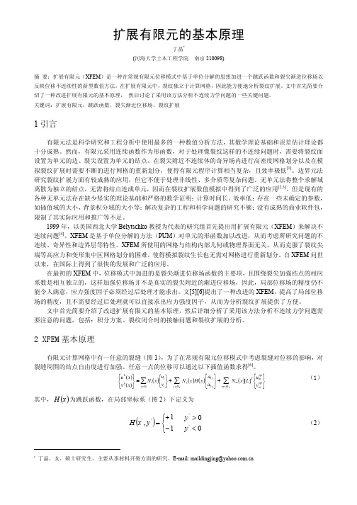
扩展有限元的基本原理
1 引言
有限元法是科学研究和工程分析中使用最多的一种数值分析方法,其数学理论基础和误差估计理论都 十分成熟。然而,有限元采用连续函数作为形函数,对于处理像裂纹这样的不连续问题时,需要将裂纹面 设置为单元的边、裂尖设置为单元的结点、在裂尖附近不连续体的奇异场内进行高密度网格划分以及在模 拟裂纹扩展时需要不断的进行网格的重新划分,使得有限元程序计算相当复杂,且效率极低[1]。边界元法 研究裂纹扩展方面有较成熟的应用,但它不便于处理非线性、多介质等复杂问题。无单元法将整个求解域 离散为独立的结点,无需将结点连成单元,因而在裂纹扩展数值模拟中得到了广泛的应用[2,3]。但是现有的 各种无单元法存在缺少坚实的理论基础和严格的数学证明; 计算时间长、 效率低; 存在一些未确定的参数, 如插值域的大小,背景积分域的大小等;解决复杂的工程和科学问题的研究不够; 没有成熟的商业软件包, 限制了其实际应用和推广等不足。 1999 年,以美国西北大学 Belytschko 教授为代表的研究组首先提出用扩展有限元(XFEM)来解决不 连续问题[4]。XFEM 是基于单位分解的方法(PUM)对单元的形函数加以改进,从而考虑所研究问题的不 连续、奇异性和边界层等特性。XFEM 所使用的网格与结构内部几何或物理界面无关,从而克服了裂纹尖 端等高应力和变形集中区网格划分的困难,使得模拟裂纹生长也无需对网格进行重新划分。自 XFEM 问世 以来,在国际上得到了很快的发展和广泛的应用。 在最初的 XFEM 中,位移模式中加进的是裂尖渐进位移场函数的主要项,且围绕裂尖加强结点的相应 系数是相互独立的,这样加强位移场并不是真实的裂尖附近的渐进位移场,因此,局部位移场的精度仍不 能令人满意,应力强度因子必须经过后处理才能求出。文[5][6]提出了一种改进的 XFEM,提高了局部位移 场的精度,且不需要经过后处理就可以直接求出应力强度因子,从而为分析裂纹扩展提供了方便。 文中首先简要介绍了改进扩展有限元的基本原理,然后详细分析了采用该方法分析不连续力学问题需 要注意的问题,包括:积分方案、裂纹闭合时的接触问题和裂纹扩展的分析。
非嵌入式多项式混沌法在爆轰产物JWL参数评估中的应用

非嵌入式多项式混沌法在爆轰产物JWL参数评估中的应用王瑞利;刘全;温万治【摘要】介绍了非嵌入多项式混沌法的数学模型,给出了非嵌入式多项式混沌法进行不确定度量化的主要步骤.采用此方法研究了平面、散心爆轰问题数值模拟中,JWL模型参数R1、R2服从均匀分布的随机变量时所引起的爆轰过程计算结果的不确度性,着重分析了爆轰传播过程中压力与密度的统计特性.研究结果表明,非嵌入式多项式混沌法可以为模型输入参数不确定性的传播对输出结果响应量的影响建立一种有效不确定度评估方法,为使用JWL模型时选取参数提供参考.【期刊名称】《爆炸与冲击》【年(卷),期】2015(035)001【总页数】7页(P9-15)【关键词】爆炸力学;JWL状态方程;参数选取;非嵌入式多项式混沌法;不确定度量化【作者】王瑞利;刘全;温万治【作者单位】北京应用物理与计算数学研究所,北京100094;北京应用物理与计算数学研究所,北京100094;北京应用物理与计算数学研究所,北京100094【正文语种】中文【中图分类】O385炸药的点火、爆轰传播研究是炸药装置设计以及安全性、可靠性研究中的重要问题。
炸药爆轰产物状态方程是描述炸药爆轰CJ状态之后的爆轰产物系统各物理量之间的关系式。
目前,已有多种爆轰产物状态方程形式,如等熵γ律状态方程、BKW及JWL状态方程[1]等。
JWL(Jones-Wilkins-Lee)状态方程的形式为:式中:P为爆轰产物的压力,v为爆轰产物的相对比容,A、B、R1、R2和w是5个待定参数。
合理确定这些参数值,才能比较精确地描述爆轰产物的膨胀驱动做功过程。
开展输入参数不确定度对输出结果不确定度传播与量化的研究是合理选取参数的重要保证。
传统用于不确定度量化的方法有蒙特卡洛法、微扰动法等[2]。
近几年,基于谱分析的多项式混沌法(polynomial chaos method, PC)[3]逐渐引起人们的注意[4-9]。
该方法根据与求解器的耦合方式,可分为嵌入式多项式混沌法(intrusive polynomial chaos, IPC)和非嵌入多项式混沌法(non-intrusive polynomial chaos, NIPC)。
基于MPI+FreeFem++的有限元并行计算

基于MPI+FreeFem++的有限元并行计算摘要:有限元方法是一种灵活而高效的数值求解偏微分方程的计算方法,是工程分析和计算中不可缺少的重要工具之一。
在计算机技术的快速发展使得并行机的价格日益下降的今天,并行有限元计算方法受到了学术界和工程界的普遍关注。
讨论了基于MPI+FreeFem++的有限元并行计算环境的构建,阐述了在该环境下有限元并行程序的编写、编译及运行等过程,并通过具体编程实例,说明了MPI+FreeFem++环境下的有限元并行编程的简单和高效。
关键词:有限元方法;并行计算;MPI;FreeFem++0 引言有限元方法是20世纪50年代伴随电子计算机的诞生,在计算数学和计算工程领域里诞生的一种高效而灵活的计算方法,它将古典变分法与分片多项式插值相结合,易于处理复杂的边值问题,具有有限差分法无可比拟的优越性,广泛应用于求解热传导、电磁场、流体力学等相关问题,已成为当今工程分析和计算中不可缺少的最重要的工具之一。
有限元方法的“化整为零、积零为整”的基本思想与并行处理技术的基本原则“分而治之”基本一致,因而具有高度的内在并行性。
在计算机技术快速发展使得并行机的价格日益下降的今天,有限元并行计算引起了学术界和工程界的普遍关注,吸引了众多科研与工程技术人员。
但要实现有限元并行编程,并不是一件容易的事,特别是对于复杂区域问题,若从网格生成、任务的划分、单元刚度矩阵的计算、总刚度矩阵的组装,到有限元方程组的求解以及后处理,都需要程序员自己编写代码的话,将是一件十分繁琐的事情。
本文探讨了构建基于MPI+FreeFem++的有限元并行计算环境,在该环境下,程序员可避免冗长代码的编写,进而轻松、快速、高效地实现复杂问题的有限元并行计算。
1 FreeFem++简介FreeFem++ 是一款免费的偏微分方程有限元计算软件,它集成网格生成器、线性方程组的求解器、后处理及计算结果可视化于一体,能快速而高效地实现复杂区域问题的有限元数值计算。
ComputationalStructuralMechanics

Argonne National Laboratory is a U.S. Department of Energy laboratory managed by UChicago Argonne, LLCComputational Structural MechanicsComputations performed on TRACC’s high-performance computers (HPCs) will greatly reduce the time for transient dynamic bridge analysis, crash analysis (auto, train,aircraft), and human injury assessment.BackgroundComputational structural mechanics is a well-established methodology for the design and analysis of many components and structures found in the transportation field. Modern computer simulation tools, such as the finite-element and meshfree methods, play a major role in these evaluations, and sophisticated commercial software codes (LS-DYNA®, LS-OPT® and Abaqus®) are available for structural analysts. These models are used to assess crashworthiness assessments of vehicles (autos, buses, trucks, trains, and aircraft) under accident conditions. Occupant models are also often included to determine occupant response and to evaluate occupant risk and the potential for developing injury reduction mechanisms.Other uses of computational structural mechanics in the transportation field include the design and analysis of important components of the highwayinfrastructure, such as bridges and roadside hardware. In these multiphysics applications, models are being developed to determine the response of bridge structures to traffic loadings; wind loadings, which may result in so-called flow-induced vibration; and hydraulic loading, which may develop during severe weather flooding of bridges. Recently, numerical studies were started to assess the structural stability of bridges with piers and abutments in scour holes. Also, attention has turned to assessing the structuralsafety of the nation’s aging steel bridges.Motor vehicle crashes are the major cause of traumatic brain injury in the United States. Numerical modeling by the NHTSA at TRACC provides valuable insight into brain response duringcrashes (image courtesy of Dr. Erik Takhounts of the NHTSA)Bridges are a critical component of the nation’s travelinfrastructure. The TFHRC is conducting simulations at TRACC to evaluate bridge safety and reliability under extreme and complex loading conditions (image courtesy of Dr. Shuang Jin of the Federal Highway Administration NDE Center).Computational Structural MechanicsAugust 2009The level of modeling detail in these applications is being increased substantially to provide greater confidence in the computed results. The use ofhigh-fidelity computational models with hundreds of thousands of elements requires the use of massively parallel computers like those at the U.S. Department of Transportation’s (USDOT’s) TransportationResearch and Analysis Computing Center (TRACC), operated by Argonne National Laboratory, and appropriate software, such as LS-DYNA, LS-OPT and Abaqus, that can take advantage of this parallel computing environment.TRACC’s SoftwareTRACC has a 280-CPU (core) license with Livermore Software and Technology Corporation for use of the LS-DYNA suite of codes and a 21-token license with Simulia for use of Abaqus. Both codes are continuously being upgraded and contain manyfeatures that can handle the complexities embedded in USDOT’s structural and media–structure interaction problems. Between the two codes the following features are available: explicit- and implicit-time integration; a robust Eigen problem solver; finite-element, extended finite-element, multi-material arbitrary Lagrangian Eulerian, and meshfreemethodologies; design optimization and probabilistic analysisFor UsersScripts for ease of use have been developed by TRACC’s expert staff and are posted on the TRACC external wiki (https:/tracc/TRACC) along with commands for checking job status. The latest information on using the code can be found on the wiki.Desktop virtualization is available to users, enabling them to interact with the cluster from a remotelocation. The NoMachine NX server is installed on the cluster and the NoMachine NX client is available at no cost to the user, providing an efficient and easy way to view finite-element models, develop and modify input files, and display computational results.TRACC’s expert staff is available for consultations on computational mechanics issues and development of collaborative projects. Staff are also available to assist with software- and HPC-related issues.Current ProjectsIn one project, the Federal Highway Administration’s Turner Fairbank Highway Research Center (TFHRC) has used TRACC’s cluster to investigate the chaotic motion of the Bill Emerson Memorial Bridge subjected to traffic loads. The finite-element model consists of more than 1 million elements. Ten days of computing time using 256 CPUs (cores) were required to simulate 100 seconds of traffic flow. In another project that is part of USDOT’s Steel Bridge TestProgram, TFHRC is assessing the structural integrity of selected steel bridges.The Human Injury Research Division of the National Highway Traffic Safety Administration (NHTSA) is working on traumatic brain injuries resulting from crashes. The TRACC cluster allows in-depth investigations that can differentiate injuries between various regions of the brain for many accident scenarios. In another project, NHTSA is usingmodeling and simulation to determine the effect of vehicle and restraint parameters on the kinematics of a crash dummy during a rollover crash simulation.The Texas Transportation Institute is analyzing and designing roadside safety features. Michigan Technological University is doing microstructure-based modeling to characterize asphalt materials and the Louisiana Transportation Research Center is simulating the performance of pavement structures for rutting performance of chemically stabilized base/subbase materials.For further information, contact TRACC Senior Computational Structural Mechanics Leader 630.578.4245*************。
图书情报全英文留学硕士研究生培养方案-武汉大学数学与统计学院

计算数学全英文留学项目博士研究生培养方案(学科代码:070102,授理学博士学位)一、培养目标本项目培养具有坚实宽广的基础知识和系统深入的专业知识的具有国际化视野的高品质、创新型计算数学领域的人才,要求具有独立从事学术研究工作的能力;并在某一方向上做深入的研究,取得创造性的成果。
二、研究方向计算数学博士项目包含偏微分方程数值解、科学与工程计算、最优控制与反问题、计算系统生物学、数据科学与大数据技术、多尺度计算6个研究方向。
1. 偏微分方程数值解主要研究偏微分方程的有限元和有限体积法以及边界积分方程的边界元法的构造、分析和实现,包括收敛性、超收敛性、后验误差控制和自适应性。
同时也对区域分解、多重网格和其它多尺度方法的分析、算法发展及应用进行研究。
2. 科学与工程计算主要研究并行算法的设计和研究,偏微分方程的并行数值方程,区域分解方法,多处理器系统中的大规模矩阵计算,并行程序环境和演示工具,高性能计算环境和PC机群,并行数值软件。
3. 最优控制与反问题主要研究偏微分方程最优控制问题的数值计算方法、随机最优控制问题的自适应方法、时间最优控制问题的理论及算法以及图像信息重构、地震构造成像和参数反演、电磁场反问题的数值求解、偏微分方程约束优化在参数估计、资料同化等方面的应用。
4. 计算系统生物学主要研究一些生物大分子(如蛋白质和DNA)静电性质以及预测某些蛋白质三维结构的数值方法的设计、分析和实现;神经信息编码和神经计算理论,神经系统的非线性动力学,神经元的数学模型,局部和大尺度神经环路的计算模拟,最优化理论和方法在基因、蛋白质序列、生物网络、生物试验设计和模型检验方面的研究和应用。
5. 数据科学与大数据技术主要研究大数据采集与挖掘、存储、处理、传输与应用等技术,及其软件与算法、数学建模与分析等。
6. 多尺度计算主要研究农业、环境和材料科学领域中多尺度问题的数学建模与理论、高效算法的设计和分析、大规模高性能并行计算技术和软件开发。
欧拉方程求解静气动弹性问题

硕士学位论文
欧拉方程求解静气动弹性问题
姓名:***
申请学位级别:硕士
专业:流体力学
指导教师:***
20050201
两北工业人学硕士学位论文第三章飞行器气动弹性问题的研究
35.Guruswamy G P ENSAERO - A Multidisciplinary Program for Fluid/Structural Interaction Studies of Aerospace Vehicles 1990(2-4)
36.Bayyuk S A.Powell K G.vail Leer B Computation of flows with moving boundaries and fluid-structure interactions.[AIAA 97- 1771] 1997
43.Davis G A.Bendiksen O O Unsteady transonic two-dimensional Euler solutions using finite elements 1993
44.Batina J T Unsteady Euler airfoil Solutions using unstructured dynamic meshes.[AIAA 89-0115] 1989
7.MacCormack R W The Effect of Viscosity on Hypervelocity Impact Cratering.[AIAA paper 69-354]
x P D.Wendroff B System of Conservation Lows
9.郑诚行.熊小依机翼跨音速非线性静气动弹性计算 1991
图灵机开发说明文档

典型图灵机的Java编程示例一图灵机概述图灵机(TM)是一种重要的计算模型,它由英国数学家A.M.Turing于1936年提出。
这个模型很好的描述了计算过程。
无数的事实表明,任何算法都可以用一个图灵机来描述,这就是著名的丘奇论题。
图灵机在可计算性理论中起着重要作用。
可以证明图灵机识别的语言就是0型语言。
图灵机的组成如下图所示:它由一个状态控制器,一个读写头和一个输入带组成。
其中输入带左右端可以无限伸长。
带上的每一格恰好有一个字符。
开始时,带上从编号为0开始的n个格存放着由有限输入字母表上的字符组成的字符串,第0格及其左边和第n+1格及其右边各格均为空白。
空白是一个特殊的带符号,它不属于输入字母表。
读写头一次可以在带上读或写一个字符,并可根据指令向左或向右移一格。
状态控制器根据当前的状态,读到输入字符并发布指令。
指令的内容包括状态转换,在带上的一格写上(更换)字符,以及读写头向左或向右移动一格等。
带子上的无穷多个小格可写、可擦;读写头可沿带子左右移动并在带上读写;每个图灵机有一个状态集Q,其中有一个开始状态和一个结束状态;还有一个符号集Σ={0,1,*};可形式化地描述为:图灵机是一个七元组M=(Q,T,Σ,δ,q0,B,H) 其中:Q ---有限的状态集合;Σ---有限的带字符集合;B ---空白符号,B∈Σ;T ---输入字符集合, T⊆Σ且B∉T;δ---下一次动作函数,是从QxΣ到QxΣx{L,R}的映射,即控制器的规则集合q0 ---初始状态,q0 ∈Q;H ---终止状态集合,H⊆Q.工作过程:首先从开始状态启动,每次动作都由控制器根据图灵机所处的当前状态和读写头所对准的符号决定下一步动作(或称操作)其中每一步包含三件事。
各符号写到读写头当前对准的那个小格内,取代原来的符号。
读写头向左或向右转动一格、或不动。
一次动作会引起:(1)控制器改变状态;(2)在当前扫描到的单元上,重写一个字符取代原来的字符;(3)读写头左移或右移一个单元;根据控制器的命令用某个状态(可以是原状态)取代当前的状态,使用图灵机进入一个新的状态。
网格计算与PC-FARM的使用

网格与中国
• 网格技术被称为网络技术发展的第三次浪潮。网络技术的前 两次浪潮(互联网和万维网),中国都没有参与世界上核心 技术的创新工作。我国的计算机产业,在总体上落后于西方 国家,一个重要原因是“文化大革命”使我们错过了参与发 明网络的前两个浪潮。
• 从1969年至今,互联网发展至今已经34年了,出现了3180个 技术标准文档(RFC)。我国科技界仅参与了一个技术标准 文档的制定。那就是1996年3月(互联网第一个标准发明27 年后,TCP/IP协议发明22年后)胡道元教授牵头制定的中文 字符编码标准(RFC 1922)。
转到作业控制窗口
每个按钮的说明(2)
每个按钮的说明(3)
2. 提交作业
脚本示例
• 运行广延大气簇射模拟程序corsika • 目录/home/wangyg/corsika • 可执行文件为qgsjet(不能直接提交) • 脚本run01.sh:
1 #!/bin/bash 2 cd ~/corsika 3 ./qgsjet<./inputs001 4
----------------------------------------------------------------------------
hgfarm4.q
BIP 1/2 0.55 glinux
74 0 run04.sh wangyg r 05/14/2003 10:45:05 MASTER
• 从1989年至今,万维网(Web)发展至今也近14年了,出现 了46个技术标准,我国科技界参与制定的技术标准一个也没 有。
• 根据Internet和Web发展的历史,网格的重要技术标准将在 2004-2005出现。这个技术将主导2004-2020年的信息技术领 域发展趋势。
meep简介
Meep(或MEEP)是一个免费的有限差分时域(FDTD)模拟软件包在麻省理工学院开发的模型电磁系统,伴随着我们MPB的本征模包。
Its features include:它的功能包括:Meep Meep发行说明Introduction简介Installation安装Tutorial教程Reference参考C++Tutorial C++教程C++Reference C++参考Acknowledgements致谢License and Copyright许可和版权•Free software under the GNU GPL.根据GNU GPL的免费软件。
•Simulation in1d,2d,3d,and cylindrical coordinates.模拟一维,二维,三维,圆柱坐标。
•Distributed memory parallelism on any system supporting the MPI standard.在任何支持的系统内存并行分布式的MPI标准。
Portable to any Unix-like system(GNU/Linux is fine).移植到任何类Unix系统(GNU/Linux的是罚款)。
•Arbitrary anisotropic electric permittivityεand magnetic permeabilityμ,along with dispersiveε(ω)andμ(ω)(including loss/gain)and nonlinear(Kerr&Pockels)dielectric and magnetic materials,and electric/magnetic conductivitiesσ.任意各向异性介电常数ε和磁导率μ,随着分散ε(ω)和μ(ω)(包括损耗/增益)和非线性(克尔电光)介电和磁材料,电/磁导率σ。
国外关于有限元方面的书籍

Ainsworth, M. and Oden, J. T., A Posterior Error Estimation in Finite Element Analysis , 2000
Backstrom, G., Fields of Physics on the PC by Finite Element Analysis, 1994
Backstrom, G., Fields of Physics by Finite Element Analysis, An Introduction, 1998
Baldwin, K., ed., Modern Methods for Automating Finite Element Mesh Generation, 1986, CP
Baran, N. M., Finite Element Analysis on Microcomputers, 1988
Argyris, J. H. and Mlejnek, H. P. Computerdynamik der Tragwerke, Band III Die Methode der Finiten Elemente, 1996
Ashwell, D. G. and Gallagher, R. H., eds. Finite Elements for Thin Shells and Curved Members, 1976
--------------------------------------------------------------------------------
biblio
Bibliography[1]FIELDVIEW Reference Manual,Software Release Version10.Intelligent Light,2004.[2]KINetics for Fluent,Version1.0.Reaction Design,Inc.,San Diego,CA,2004.[3]P.J.O’Rourke A.A.Amsden and T.D.Butler.KIVA-2:A Computer Program forChemically Reactive Flows with Sprays.Technical Report LA-11560-MS,UC-96, Los Alamos National Laboratory,Los Alamos,New Mexico,May1989.[4]A.Perera A.Antifora,M.Sala and L.Vigevano.NO x Emissions in CombustionSystems of Coal Fired Furnaces with a Reducing Environment:Predictions and Measurements.In Fourth International Conference on Technologies and Combus-tion for a Clean Environment,Lisbon,Portugal,1997.[5]T.Ahmad,S.L.Plee,and putation of Nitric Oxide and SootEmissions from Turbulent Diffusion Flames.J.of Engineering for Gas Turbines and Power,107:48–53,1985.[6]B.J.Alder and T.E.Wainright.Studies in Molecular Dynamics.II:Behaviour ofSmall Number of Spheres.J.Chem.Phys.,33:1439,1960.[7]B.J.Alder and T.E.Wainwright.Studies in Molecular Dynamics II:Behaviourof a Small Number of Elastic Spheres.J.Chem.Phys.,33:1439,1990.[8]A.A.Amsden.KIVA-3:A KIVA Program with Block-Structured Mesh for Com-plex Geometries.Technical Report LA-12503-MS,UC-361,Los Alamos National Laboratory,Los Alamos,New Mexico,March1993.[9]T.B.Anderson and R.Jackson.A Fluid Mechanical Description of Fluidized Beds.I&EC Fundam.,6:527–534,1967.[10]S.Armsfield and R.Street.The Fractional-Step Method for the Navier-StokesEquations on Staggered Grids:Accuracy of Three Variations.Journal of Compu-tational Physics,153:660–665,1999.[11]R.H.Augnier.A Fast,Accurate Real Gas Equation of State for Fluid DynamicAnalysis Applications.Journal of Fluids Engineering,117:277–281,1995.[12]F.Backmier,K.H.Eberius,and b.Sci.Tech.,7:77,1973.BIBLIOGRAPHY[13]S.Badzioch and P.G.W.Hawksley.Kinetics of Thermal Decomposition of Pulver-ized Coal Particles.Ind.Eng.Chem.Process Design and Development,9:521–530,1970.[14]R.S.Barlow,G.J.Fiechtner,C.D.Carter,and J.Y.Chen.Experiments onthe Scalar Structure of Turbulent CO/H2/N2Jet bustion and Flame,120:549–569,2000.[15]F.J.Barnes,J.H.Bromly,T.J.Edwards,and R.Madngezewsky.NO x Emissionsfrom Radiant Gas Burners.Journal of the Institute of Energy,155:184–188,1988.[16]R.Barrett,M.Berry,T.F.Chan,J.Demmel,J.Donato,J Dongarra,V.Eijkhout,R.Pozo,C.Romine,and H.Van der Vorst.Templates for the Solution of LinearSystems:Building Blocks for Iterative Methods.SIAM,Philadelphia,Pennsylvania,2nd edition edition,1994.[17]T.J.Barth and D.Jespersen.The design and application of upwind schemeson unstructured meshes.Technical Report AIAA-89-0366,AIAA27th AerospaceSciences Meeting,Reno,Nevada,1989.[18]H.Barths,C.Antoni,and N.Peters.Three-Dimensional Simulation of PollutantFormation in a DI-Diesel Engine Using Multiple Interactive Flamelets.SAE Paper,accepted for publication1998.[19]H.Barths et al.Simulation of Pollutant Formation in a Gas Turbine CombustorUsing Unsteady Flamelets.In27th Symp.(Int’l.)on Combustion.The CombustionInstitute,accepted for publication1998.[20]G.K.Batchelor.An Introduction to Fluid Dynamics.Cambridge Univ.Press,Cambridge,England,1967.[21]D.L.Baulch,D.D.Drysdall,D.G.Horne,and A.C.Lloyd.Evaluated KineticData for High Temperature Reactions,volume1,2,3.Butterworth,1973.[22]D.L.Baulch et al.Evaluated Kinetic Data for Combustion Modelling.J.Physicaland Chemical Reference Data,21(3),1992.[23]M.M.Baum and P.J.Street.Predicting the Combustion Behavior of Coal Parti-bust.Sci.Tech.,3(5):231–243,1971.[24]L.L.Baxter.Turbulent Transport of Particles.PhD thesis,Brigham Young Uni-versity,Provo,Utah,1989.[25]L.L.Baxter and P.J.Smith.Turbulent Dispersion of Particles:The STP Model.Energy&Fuels,7:852–859,1993.[26]W.Bechara,C.Bailly,fon,and S.Candel.Stochastic Approach to NoiseModeling for Free Turbulent Flows.AIAA Journal,32:3,1994.BIBLIOGRAPHY [27]M.Behnia,S.Parneix,Y.Shabany,and P.A.Durbin.Numerical Study of Tur-bulent Heat Transfer in Confined and Unconfined Impinging Jets.International Jounal of Heat and Fluid Flow,20:1–9,1999.[28]A.Bejan.Convection Heat Transfer.John Wiley and Sons,New York,1984.[29]R.W.Bilger and R.E.Beck.In15th Symp.(Int’l.)on Combustion,page541.TheCombustion Institute,1975.[30]R.W.Bilger,M.B.Esler,and S.H.Starner.On Reduced Mechanisms for Methane-Air Combustion.In Lecture Notes in Physics,volume384,page86.Springer-Verlag, 1991.[31]B.Binniger,M.Chan,G.Paczkko,and M.Herrmann.Numerical Simulation ofTurbulent Partially Premixed Hydrogen Flames with the Flamelet Model.Techni-cal report,Advanced Combustion Gmbh,Internal Report,1998.[32]J.Blauvens,B.Smets,and J.Peters.In16th Symp.(Int’l.)on Combustion.TheCombustion Institute,1977.[33]R.M.Bowen.Theory of Mixtures.In A.C.Eringen,editor,Continuum Physics,pages1–127.Academic Press,New York,1976.[34]C.T.Bowman.Chemistry of Gaseous Pollutant Formation and Destruction.InW.Bartok and A.F.Sarofim,editors,Fossil Fuel Combustion.J.Wiley and Sons, Canada,1991.[35]R.K.Boyd and J.H.Kent.Three-dimensional furnace computer modeling.In21stSymp.(Int’l.)on Combustion,pages265–274.The Combustion Institute,1986. [36]J.U.Brackbill,D.B.Kothe,and C.Zemach.A Continuum Method for ModelingSurface put.Phys.,100:335–354,1992.[37]A.Brandt.Multi-level Adaptive Computations in Fluid Dynamics.TechnicalReport AIAA-79-1455,AIAA,Williamsburg,VA,1979.[38]K.N.Bray and minar Flamelets in Turbulent Flames.In P.A.Libbyand F.A.Williams,editors,Turbulent Reacting Flows,pages63–114.Academic Press,1994.[39]K.S.Brentner and F.Farassat.An Analytical Comparison of the Acoustic Analogyand KirchhoffFormulations for Moving Surfaces.AIAA Journal,36(8),1998. [40]J.Brouwer,M.P.Heap,D.W.Pershing,and P.J.Smith.A Model for Predictionof Selective Non-Catalytic Reduction of Nitrogen Oxides by Ammonia,Urea,and Cyanuric Acid with Mixing Limitations in the Presence of CO.In26th Symposium (Int’l)on Combustion,The Combustion Institute,1996.BIBLIOGRAPHY[41]S.Brunauer.The Absorption of Gases and Vapors.Princeton University Press,Princeton,NJ,1943.[42]Trong T.Bui.A Parallel,Finite-Volume Algorithm for Large-Eddy Simulation ofTurbulent Flows.Technical Memorandum NASA/TM-1999-206570,1999.[43]M.Sommerfeld C.Mundo and C.Tropea.Droplet-Wall Collisions:ExperimentalStudies of the Deformation and Breakup Process.International Journal of Multi-phase Flow,21(2):151–173,1995.[44]R.Cao and S.B.Pope.Numerical Integration of Stochastic Differential Equations:Weak Second-Order Mid-Point Scheme for Application in the Composition PDFMethod.Journal of Computational Physics,185(1):194–212,2003.[45]N.F.Carnahan and K.E.Starling.Equations of State for Non-Attracting RigidSpheres.J.Chem.Phys.,51:635–636,1969.[46]M.G.Carvalho,T.Farias,and P.Fontes.Predicting Radiative Heat Transfer inAbsorbing,Emitting,and Scattering Media Using the Discrete Transfer Method.In W.A.Fiveland et al.,editor,Fundamentals of Radiation Heat Transfer,volume160,pages17–26.ASME HTD,1991.[47]J.R.Cash and A.H.Karp.A variable order Runge-Kutta method for initial valueproblems with rapidly varying right-hand sides.ACM Transactions on Mathemat-ical Software,16:201–222,1990.[48]T.Cebeci and P.Bradshaw.Momentum Transfer in Boundary Layers.HemispherePublishing Corporation,New York,1977.[49]S.Chapman and T.G.Cowling.The Mathematical Theory of Non-Uniform Gases.Cambridge University Press,Cambridge,England,3rd edition,1990.[50]S.Charpenay,M.A.Serio,and P.R.Solomon.In24th Symp.(Int’l.)on Combus-tion,pages1189–1197.The Combustion Institute,1992.[51]H.C.Chen and V.C.Patel.Near-Wall Turbulence Models for Complex FlowsIncluding Separation.AIAA Journal,26(6):641–648,1988.[52]P.Cheng.Two-Dimensional Radiating Gas Flow by a Moment Method.AIAAJournal,2:1662–1664,1964.[53]N.P.Cheremisinoff.Fluid Flow Pocket Handbook.Gulf Publishing Co.,Houston,TX.,1984.[54]D.Choudhury.Introduction to the Renormalization Group Method and TurbulenceModeling.Fluent Inc.Technical Memorandum TM-107,1993.BIBLIOGRAPHY [55]E.H.Chui and putation of Radiant Heat Transfer on a Non-Orthogonal Mesh Using the Finite-Volume Method.Numerical Heat Transfer,Part B,23:269–288,1993.[56]Clift,Grace,and Weber.Bubbles,Drops,and Particles.Technical report,AcademicPress,1978.[57]P.J.Coelho and M.G.Carvalho.Modelling of Soot Formation and Oxidation inTurbulent Diffusion Flames.J.of Thermophysics and Heat Transfer,9(4):644–652, 1995.[58]M.F.Cohen and D.P.Greenberg.The Hemi-Cube:A Radiosity Solution forComplex puter Graphics,19(3):31–40,1985.[59]D.Cokljat,V.A.Ivanov,F.J.Sarasola,and S.A.Vasquez.Multiphase k-epsilonModels for Unstructured Meshes.In ASME2000Fluids Engineering Division Sum-mer Meeting,Boston,USA,2000.[60]A.Coppalle and P.Vervisch.The Total Emissivities of High-Temperature Flames.Combust.Flame,49:101–108,1983.[61]S.M.Correa.A Review of NO x Formation Under Gas-Turbine Combustion Con-bustion Science and Technology,87:329–362,1992.[62]C.Crowe,M.Sommerfield,and Yutaka Tsuji.Multiphase Flows with Droplets andParticles.CRC Press,1998.[63]G.T.Csanady.Turbulent Diffusion of Heavy Particles in the Atmosphere.J.Atmos.Science,20:201–208,1963.[64]N.Curle.The Influence of Solid Boundaries upon Aerodynamic Sound.Proceedingsof the Royal Society of London.Series A,Mathematical and Physical Sciences, 231:505–514,1955.[65]E.H.Cuthill and J.McKee.Reducing Bandwidth of Sparse Symmetric Matrices.In Proc.ACM24th National Conf.,pages157–172,New York,1969.[66]M.Slack D.Cokljat and S.A.Vasquez.Reynolds-Stress Model for Eulerian Multi-phase.In Y.Nagano K.Hanjalic and M.J.Tummers,editors,Proceedings of the4th International Symposium on Turbulence Heat and Mass Transfer,pages1047–1054.Begell House,Inc.,2003.[67]J.Dacles-Mariani,G.G.Zilliac,J.S.Chow,and P.Bradshaw.Numeri-cal/Experimental Study of a Wingtip Vortex in the Near Field.AIAA Journal, 33(9):1561–1568,1995.[68]J.M.Dalla Valle.Micromeritics.Pitman,London,1948.BIBLIOGRAPHY[69]B.J.Daly and F.H.Harlow.Transport Equations in Turbulence.Phys.Fluids,13:2634–2649,1970.[70]J.F.Daunenhofer and J.R.Baron.Grid Adaption for the2D Euler Equations.Technical Report AIAA-85-0484,American Institute of Aeronautics and Astronau-tics,1985.[71]J.E.Dec.A Conceptual Model of DI Diesel Combustion Based on Laser SheetImaging.SAE Technical Paper970873,SAE,1997.[72]M.K.Denison and B.W.Webb.A Spectral Line-Based Weighted-Sum-of-Gray-Gases Model for Arbitrary RTE Solvers.J.Heat Transfer,115:1002–1012,1993.[73]J.Ding and D.Gidaspow.A Bubbling Fluidization Model Using Kinetic Theoryof Granular Flow.AIChE J.,36(4):523–538,1990.[74]G.Dixon-Lewis.Structure of Laminar Flames.In23rd Symp.(Int’l.)on Combus-tion,pages305–324.The Combustion Institute,1990.[75]N.Dombrowski and P.C.Hooper.The effect of ambient density or drop formationin sprays.Chemical Engineering Science,17:291–305,1962.[76]N.Dombrowski and W.R.Johns.The aerodynamic Instability and Disintegrationof Viscous Liquid Sheets.Chemical Engineering Science,18:203,1963.[77]C.Dopazo and E.E.O’Brien.Functional formulation of nonisothermal turbulentreactiveflows.Phys.Fluids,17:1968,1975.[78]A.M.Douaud and P.Eyzat.Four-Octane-Number Method for Predicting theAnti-Knock Behavior of Fuels in Engines.SAE Technical Paper,v87780080,SAE,1978.[79]M.C.Drake and R.J.Blint.Relative Importance of Nitrogen Oxide FormationMechanisms in Laminar Opposed-Flow Diffusion bustion and Flame,83:185–203,1991.[80]M.C.Drake,S.M.Correa,R.W.Pitz,W.Shyy,and C.P.Fenimore.Superequi-librium and Thermal Nitric Oxide Formation in Turbulent Diffusion -bustion and Flame,69:347–365,1987.[81]M.C.Drake,R.W.Pitz,pp,C.P.Fenimore,R.P.Lucht,D.W.Sweeney,and urendeau.In20th Symp.(Int’l.)on Combustion,page327.TheCombustion Institute,1984.[82]D.A.Drew and hey.In Particulate Two-Phase Flow,pages509–566.Butterworth-Heinemann,Boston,1993.BIBLIOGRAPHY [83]J.K.Dukowwicz and A.S.Dvinsky.Approximate Factorization as a High-OrderSplitting for the Implicit Incompressible Flow Equations.Journal of Computational Physics,102:336–347,1992.[84]P.A.Durbin.Separated Flow Computations with the k- -v2Model.AIAA Journal,33(4):659–664,1995.[85]V.N.Vatsa E.Turkel.Choice of variables and preconditioning for time depen-dent problems.Technical Report AIAA-2003-3692,American Institute of Aero-nautics and Astronautics,16th AIAA Computational Fluid Dynamics Conference, Orlando,Florida,June2003.[86]E.R.G.Eckert and R.M.Drake.Analysis of Heat and Mass Transfer.McGraw-HillCo.,1972.[87]D.K.Edwards and R.Matavosian.Scaling Rules for Total Absorptivity and Emis-sivity of Gases.J.Heat Transfer,106:684–689,1984.[88]J.K.Edwards,K.Jeremy,B.S.McLaury,S.Brenton,S.A.Shirazi,and A.Sia-mack.Supplementing a CFD Code with Erosion Prediction Capabilities.In Pro-ceedings of ASME FEDSM’98:ASME1998Fluids Engineering Division Summer Meeting,Washington D.C.,June1998.[89]J.K.Edwards,B.S.McLaury,and S.A.Shirazi.Evaluation of Alternative PipeBend Fittings in Erosive Service.In Proceedings of ASME FEDSM’00:ASME 2000Fluids Engineering Division Summer Meeting,Boston,June2000.[90]S.E.Elgobashi and T.W.Abou-Arab.A Two-Equation Turbulence Model forTwo-Phase Flows.Phys.Fluids,26(4):931–938,1983.[91]S.Ergun.Fluid Flow through Packed Columns.Chem.Eng.Prog.,48(2):89–94,1952.[92]G.M.Faeth.Spray Atomization and Combustion.AIAA Journal,(86-0136),1986.[93]R.F.Fedors and ndell.An Empirical Method of Estimating the VoidFraction in Mixtures of Uniform Particles of Different Size.Powder Technology, 23:225–231.[94]C.P.Fenimore.Formation of Nitric Oxide in Premixed Hydrocarbon Flames.In13th Symp.(Int’l.)on Combustion,page373.The Combustion Institute,1971. [95]C.P.Fenimore.Destruction of NO by NH3in Lean Burnt bustion andFlame,37:245,1980.[96]J.L.Ferzieger and putational Methods for Fluid Dynamics.Springer-Verlag,Heidelberg,1996.BIBLIOGRAPHY[97]J.E.Ffowcs-Williams and D.L.Hawkings.Sound Generation by Turbulence andSurfaces in Arbitrary Motion.Proc.Roy.Soc.London,A264:321–342,1969.[98]M.A.Field.Rate of Combustion Of Size-Graded Fractions of Char from a LowRank Coal between1200K–bust.Flame,13:237–252,1969.[99]I.Finnie.Erosion of Surfaces by Solid Particles.Wear,3:87–103,1960.[100]W.A.Fiveland and A.S.Jamaluddin.Three-Dimensional Spectral Radiative Heat Transfer Solutions by the Discrete Ordinates Method.HTD Vol.106,Heat TransferPhenomena in Radiation,Combustion and Fires,pp.43–48,1989.[101]T.H.Fletcher and pilation of Sandia coal devolatilization data:Milestone report.Sandia Report SAND92-8209,1992.[102]T.H.Fletcher and A.R.Kerstein.Chemical percolation model for devolatilization:3.Direct use of13C NMR data to predict effects of coal type.Energy and Fuels,6:414,1992.[103]T.H.Fletcher,A.R.Kerstein,R.J.Pugmire,and D.M.Grant.Chemical percola-tion model for devolatilization:2.Temperature and heating rate effects on productyields.Energy and Fuels,4:54,1990.[104]W.L.Flower,R.K.Hanson,and C.H.Kruger.In15th Symp.(Int’l.)on Com-bustion,page823.The Combustion Institute,1975.[105]S.Fu,under,and M.A.Leschziner.Modeling Strongly Swirling Recircu-lating Jet Flow with Reynolds-Stress Transport Closures.In Sixth Symposium onTurbulent Shear Flows,Toulouse,France,1987.[106]J.Garside and M.R.Al-Dibouni.Velocity-Voidage Relationships for Fluidization and Sedimentation.I&EC Process Des.Dev.,16:206–214,1977.[107]M.Germano,U.Piomelli,P.Moin,and W.H.Cabot.Dynamic Subgrid-Scale Eddy Viscosity Model.In Summer Workshop,Center for Turbulence Research,Stanford,CA,1996.[108]T.Gessner.Dynamic Mesh Adaption for Supersonic Combustion Waves Modeled with Detailed Reaction Mechanisms.PhD thesis,University of Freiburg,Freiburg,Germany,2001.[109]N.E.Gibbs,W.G.Poole,Jr.,and P.K.Stockmeyer.An algorithm for reducing the bandwidth and profile of a sparse matrix.SIAM J.Numer.Anal.,13:236–250,1976.[110]M.M.Gibson and under.Ground Effects on Pressure Fluctuations in the Atmospheric Boundary Layer.J.Fluid Mech.,86:491–511,1978.BIBLIOGRAPHY[111]D.Gidaspow.Multiphase Flow and Fluidization.Academic Press,Boston,1994. [112]D.Gidaspow,R.Bezburuah,and J.Ding.Hydrodynamics of Circulating Flu-idized Beds,Kinetic Theory Approach.In Fluidization VII,Proceedings of the7th Engineering Foundation Conference on Fluidization,pages75–82,1992.[113]R.G.Gilbert,K.Luther,and J.Troe.Ber.Bunsenges.Phys.Chem.,87,1983. [114]M.Giles.Non-Reflecting Boundary Conditions for the Euler Equations.Technical Report TR88-1-1988,Computational Fluid Dynamics Laboratory,Massachusetts Institute of Technology,Cambridge,MA.[115]P.Glarborg,J.E.Johnsson,and K.Dam-Johansen.Kinetics of Homogeneous Nitrous Oxide bustion and Flame,99:523–532,1994. [116]M.E.Goldstein and B.Rosenbaum.Effect of Anisotropic Turbulence on Aerody-namic Noise.Journal of the Acoustical Society of America,54:630–645,1973.[117]J.Gottgens,F.Mauss,and N.Peters.Analytic Approximations of Burning Ve-locities and Flame Thicknesses of Lean Hydrogen,Methane,Ethylene,Ethane, Acetylene and Propane Flames.In Twenty-Fourth Symposium(Int.)on Combus-tion,pages129–135,Pittsburgh,1992.[118]I.R.Gran and B.F.Magnussen.A numerical study of a bluff-body stabilized diffusionflame.part2.influence of combustion modeling andfinite-rate chemistry.Combustion Science and Technology,119:191,1996.[119]D.M.Grant,R.J.Pugmire,T.H.Fletcher,and A.R.Kerstein.Chemical per-colation model of coal devolatilization using percolation lattice statistics.Energy and Fuels,3:175,1989.[120]P.M.Gresho,R.L.Lee,and R.L.Sani.On the Time-Dependent Solution of the Incompressible Navier-Stokes Equations in Two and Three Dimensions.In Recent Advances in Numerical Methods in Fluids.Pineridge Press,Swansea,U.K.,1980. [121]D.J.Gunn.Transfer of Heat or Mass to Particles in Fixed and Fluidized Beds.Int.J.Heat Mass Transfer,21:467–476,1978.[122]W.W.Hagerty and J.F.Shea.A Study of the Stability of Plane Fluid Sheets.Journal of Applied Mechanics,22:509,1955.[123]A.Haider and O.Levenspiel.Drag Coefficient and Terminal Velocity of Spherical and Nonspherical Particles.Powder Technology,58:63–70,1989.[124]Z.Han,S.Perrish,P.V.Farrell,and R.D.Reitz.Modeling Atomization Processes of Pressure-Swirl Hollow-Cone Fuel Sprays.Atomization and Sprays,7(6):663–684, Nov.-Dec.1997.BIBLIOGRAPHY[125]G.Hand,M.Missaghi,M.Pourkashanian,and A.Williams.Experimental Studies and Computer Modelling of Nitrogen Oxides in a Cylindrical Furnace.In Pro-ceedings of the Ninth Members Conference,volume2.IFRF Doc No K21/g/30,1989.[126]R.K.Hanson and S.Salimian.Survey of Rate Constants in H/N/O Systems.In W.C.Gardiner,editor,Combustion Chemistry,page361,1984.[127]H.O.Hardenburg and F.W.Hase.An Empirical Formula for Computing the Pressure Rise Delay of a Fuel from its Cetane Number and from the RelevantParameters of Direct Injection Diesel Engines.SAE Technical Paper790493,SAE,1979.[128]R.A.W.M.Henkes and C.J.Hoogendoorn.Scaling of the Turbulent Natural Convection Flow in a Heated Square Cavity.Trans.of the ASME,116:400–408,May1994.[129]R.A.W.M.Henkes,F.F.van der Flugt,and C.J.Hoogendoorn.Natural Convec-tion Flow in a Square Cavity Calculated with Low-Reynolds-Number TurbulenceModels.Int.J.Heat Mass Transfer,34:1543–1557,1991.[130]J.B.Heywood.Internal Combustion Engine Fundamentals.McGraw-Hill,New York,rev.edition,1988.[131]J.O.Hinze.Turbulence.McGraw-Hill Publishing Co.,New York,1975.[132]C.Hirsch.Numerical Computation of Internal and External Flows:Computational Methods for Inviscid and Viscous Flows,volume2.John Wiley&Sons,New York,1984.[133]J.O.Hirschfelder,C.F.Curtiss,and R.B.Bird.Molecular Theory of Gases and Liquids.John Wiley&Sons,New York,1954.[134]C.W.Hirt and B.D.Nichols.Volume of Fluid(VOF)Method for the Dynamics of Free put.Phys.,39:201–225,1981.[135]D.G.Holmes and S.D.Connell.Solution of the2D Navier-Stokes Equations on Unstructured Adaptive Grids.Presented at the AIAA9th Computational FluidDynamics Conference,June,1989.[136]T.J.Houser,M.Hull,R.Alway,and T.Biftu.Int.Journal of Chem.Kinet., 12:579,1980.[137]P.Huang,P.Bradshaw,and T.Coakley.Skin Friction and Velocity Profile Family for Compressible Turbulent Boundary Layers.AIAA Journal,31(9):1600–1604,September1993.[138]B.R.Hutchinson and G.D.Raithby.A Multigrid Method Based on the Additive Correction Strategy.Numerical Heat Transfer,9:511–537,1986.[139]Hadjira Ibdir and Hamid Arastoopour.Modeling of multi-type particleflow using kinetic approach.AICHE Journal,May2005.[140]R.I.Issa.Solution of Implicitly Discretized Fluid Flow Equations by Operator put.Phys.,62:40–65,1986.[141]R.I.Issa.Solution of the Implicitly Discretized Fluid Flow Equations by Operator-Splitting.Journal of Computational Physics,62:40–65,1985.[142]G.W.Jackson and D.F.James.The Permeability of Fibrous Porous Media.Canadian Journal of Chem.Eng.,64(3):364–374,June1986.[143]S.Jain.Three-Dimensional Simulation of Turbulent Particle Dispersion.PhD thesis,University of Utah,Utah,1995.[144]A.Jameson.Solution of the Euler Equations for Two Dimensional Transonic Flow by a Multigrid Method.MAE Report1613,Princeton University,June1983.[145]A.Jameson,W.Schmidt,and E.Turkel.Numerical Solution of the Euler Equations by Finite Volume Methods Using Runge-Kutta Time-Stepping Schemes.Technical Report AIAA-81-1259,AIAA14th Fluid and Plasma Dynamics Conference,Palo Alto,California,June1981.[146]J Janicka,W.Kolbe,and W.Kollmann.Closure of the transport equation for the pdf of turbulent scalarfields.Journal Non-Equilibrium Thermodynamics,4:47, 1978.[147]J.Janicka and W.Kollmann.A Two-Variable Formulation for the Treatment of Chemical Reactions in Turbulent H2-Air Diffusion Flames.In17th Symp.(Int’l.) on Combustion.The Combustion Institute,1978.[148]J.Janicka and W.Kollmann.A Numerical Study of Oscillating Flow Around a Circular bustion and Flame,44:319–336,1982.[149]C.Jayatilleke.The Influence of Prandtl Number and Surface Roughness on the Resistance of the Laminar Sublayer to Momentum and Heat Transfer.Prog.Heat Mass Transfer,1:193–321,1969.[150]H.M.Glaz J.B.Bell,P.Colella.Second-Order Projection Method for the Incom-pressible Navier-Stokes Equations.Journal of Computational Physics,85:257,1989. [151]H.M.Glaz J.B.Bell,P.Colella.An Analysis of the Fractional-Step Method.Journal of Computational Physics,108:51–58,1993.[152]P.C.Johnson and R.Jackson.Frictional-Collisional Constitutive Relations for Granular Materials,with Application to Plane Shearing.J.Fluid Mech.,176:67–93,1987.[153]W.P.Jones and J.H.Whitelaw.Calculation Methods for Reacting Turbulent Flows:A bust.Flame,48:1–26,1982.[154]T.Jongen.Simulation and Modeling of Turbulent Incompressible Flows.PhD thesis,EPF Lausanne,Lausanne,Switzerland,1992.[155]T.Just and S.Kelm.Die Industry,38:76,1986.[156]A.Ronald K.Haugen,O.Kvernvold and R.Sandberg.Sand Erosion of Wear-resistant Materials:Erosion in Choke Valves.Wear,186-187:179–188,1995.[157]H.Daiguji K.Ishazaki,T.Ikohagi.A High-Resolution Numerical Method for Tran-sonic Non-equilibrium Condensation Flows Through a Steam Turbine Cascade.In Proceedings of the6th International Symposium on Computational Fluid Dynamics, volume1,pages479–484,1995.[158]B.Kader.Temperature and Concentration Profiles in Fully Turbulent Boundary Layers.Int.J.Heat Mass Transfer,24(9):1541–1544,1981.[159]N.Kandamby,zopoulos,F.C.Lockwood,A.Perera,and L.Vigevano.Math-ematical Modeling of NO x Emission Reduction by the Use of Reburn Technology in Utility Boilers.In ASME Int.Joint Power Generation Conference and Exhibition, Houston,Texas,1996.[160]K.C.Karki and S.V.Patankar.Pressure-Based Calculation Procedure for Viscous Flows at All Speeds in Arbitrary Configurations.AIAA Journal,27:1167–1174, 1989.[161]G.Karypis and V.Kumar.METIS-A Software Package for Partitioning Un-structured Graphs,Partitioning Meshes,and Computing Fill-Reducing Orderings of Sparse Matrices,Version3.0.Manual,University of Minnesota and Army HPC Research Center,1997.[162]W.M.Kays.Loss coefficients for abrupt changes inflow cross section with low reynolds numberflow in single and multiple tube systems.Transactions of the ASME,72:1067–1074,January1950.[163]W.M.Kays.Turbulent Prandtl Number-Where Are We?J.Heat Transfer, 116:284–295,1994.[164]W.M.Kays and pact Heat Exchangers.McGraw-Hill,New York,1964.[165]R.J.Kee,F.M.Rupley,ler,M.E.Coltrin,J.F.Grcar,E.Meeks,H.K.Moffat,A.E.Lutz,G.Dixon-Lewis,M.D.Smooke,J.Warnatz,G.H.Evans, rson,R.E.Mitchell,L.R.Petzold,W.C.Reynolds,M.Caracotsios, W.E.Stewart,P.Glarborg,C.Wang,O.Adigun,W.G.Houf,C.P.Chou,S.F.Miller,P.Ho,and D.J.Young.CHEMKIN v.4.0.Technical Report San Diego, CA,Reaction Design,Inc.,2004.[166]R.J.Kee,F.M.Rupley,and ler.SURFACE CHEMKIN:A Software Pack-age for the Analysis of Heterogeneous Chemical Kinetics at a Solid-Surface-Gas-Phase Interface.Technical Report SAND96-8217,Sandia National Labs,2000.[167]I.M.Khan and G.Greeves.A Method for Calculating the Formation and Com-bustion of Soot in Diesel Engines.In N.H.Afgan and J.M.Beer,editors,Heat Transfer in Flames,chapter25.Scripta,Washington DC,1974.[168]J.S.Kim and F.A.Williams.Extinction of Diffusion Flames with Non-Unity Lewis Number.Eng.Math,31:101–118,1997.[169]rge eddy simulation using unstructured meshes and dynamic subgrid-scale turbulence models.Technical Report AIAA-2004-2548,American Institute of Aeronautics and Astronautics,34th Fluid Dynamics Conference and Exhibit,June 2004.[170]S.-E.Kim and D.Choudhury.A Near-Wall Treatment Using Wall Functions Sensi-tized to Pressure Gradient.In ASME FED Vol.217,Separated and Complex Flows.ASME,1995.[171]S.-E.Kim,D.Choudhury,and putations of Complex Turbulent Flows Using the Commercial Code FLUENT.In Proceedings of the ICASE/LaRC/AFOSR Symposium on Modeling Complex Turbulent Flows,Hampton,Virginia,1997. [172]W.-W.Kim and S.Menon.Application of the localized dynamic subgrid-scale model to turbulent wall-boundedflows.Technical Report AIAA-97-0210,American Institute of Aeronautics and Astronautics,35th Aerospace Sciences Meeting,Reno, NV,January1997.[173]H.Kobayashi,J.B.Howard,and A.F.Sarofim.Coal Devolatilization at High Temperatures.In16th Symp.(Int’l.)on Combustion.The Combustion Institute, 1976.[174]R.Kraichnan.Diffusion by a Random Velocity Field.Physics of Fluids,11:21–31, 1970.[175]K.K.Y.Kuo.Principles of Combustion.John Wiley and Sons,New York,1986.[176]V.R.Kuznetsov and V.A.Sabelnikov.Turbulence and Combustion,1990.[177]mb.Hydrodynamics,Sixth Edition.Dover Publications,New York,1945.[178]rsen and J.R.Howell.Least Squares Smoothing of Direct Exchange Areas in Zonal Analysis.J.Heat Transfer,108:239–242,1986.[179]under.Second-Moment Closure and Its Use in Modeling Turbulent In-dustrial Flows.International Journal for Numerical Methods in Fluids,9:963–985, 1989.[180]under.Second-Moment Closure:Present...and Future?Inter.J.Heat Fluid Flow,10(4):282–300,1989.[181]under,G.J.Reece,and W.Rodi.Progress in the Development of a Reynolds-Stress Turbulence Closure.J.Fluid Mech.,68(3):537–566,April1975.[182]under and N.Shima.Second-Moment Closure for the Near-Wall Sublayer: Development and Application.AIAA Journal,27(10):1319–1325,1989.[183]under and D.B.Spalding.Lectures in Mathematical Models of Turbulence.Academic Press,London,England,1972.[184]under and D.B.Spalding.The Numerical Computation of Turbulent Flows.Computer Methods in Applied Mechanics and Engineering,3:269–289,1974.[185]urendeau.Heterogeneous Kinetics of Coal Char Gasification and Com-bustion.Prog.Energy Comb.Sci.,4:221–270,1978.[186]J.L.Lebowitz.Exact Solution of Generalized Percus-Yevick Equation for a Mixture of Hard Spheres.The Phy.Rev.,133(4A):A895–A899,1964.[187]A.H.Lefebvre.Atomization and Sprays.Hemisphere Publishing Corporation, 1989.[188]B.P.Leonard and S.Mokhtari.ULTRA-SHARP Nonoscillatory Convection Schemes for High-Speed Steady Multidimensional Flow.NASA TM1-2568 (ICOMP-90-12),NASA Lewis Research Center,1990.[189]B.P.Leonard.The ULTIMATE conservative difference scheme applied to unsteady one-dimensional p.Methods Appl.Mech.Eng.,88:17–74,1991. [190]K.M.Leung and R.P.Lindsted.Detailed Kinetic Modeling of C1-C3Alkane Diffusion bustion and Flame,102:129–160,1995.[191]J.M.Levy,L.K.Chen,A.F.Sarofim,and J.M.Beer.NO/Char Reactions at Pulverized Coal Flame Conditions.In18th Symp.(Int’l.)on Combustion.The Combustion Institute,1981.[192]A.Li and G.Ahmadi.Dispersion and Deposition of Spherical Particles from Point Sources in a Turbulent Channel Flow.Aerosol Science and Technology,16:209–226, 1992.。
目标函数误差估算及网格自适应处理
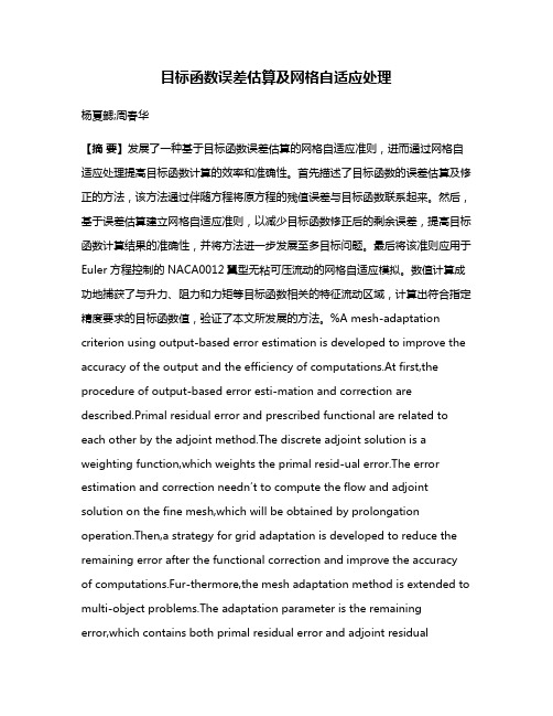
目标函数误差估算及网格自适应处理杨夏勰;周春华【摘要】发展了一种基于目标函数误差估算的网格自适应准则,进而通过网格自适应处理提高目标函数计算的效率和准确性。
首先描述了目标函数的误差估算及修正的方法,该方法通过伴随方程将原方程的残值误差与目标函数联系起来。
然后,基于误差估算建立网格自适应准则,以减少目标函数修正后的剩余误差,提高目标函数计算结果的准确性,并将方法进一步发展至多目标问题。
最后将该准则应用于Euler 方程控制的 NACA0012翼型无粘可压流动的网格自适应模拟。
数值计算成功地捕获了与升力、阻力和力矩等目标函数相关的特征流动区域,计算出符合指定精度要求的目标函数值,验证了本文所发展的方法。
%A mesh-adaptation criterion using output-based error estimation is developed to improve the accuracy of the output and the efficiency of computations.At first,the procedure of output-based error esti-mation and correction are described.Primal residual error and prescribed functional are related to each other by the adjoint method.The discrete adjoint solution is a weighting function,which weights the primal resid-ual error.The error estimation and correction needn′t to compute the flow and adjoint solution on the fine mesh,which will be obtained by prolongation operation.Then,a strategy for grid adaptation is developed to reduce the remaining error after the functional correction and improve the accuracy of computations.Fur-thermore,the mesh adaptation method is extended to multi-object problems.The adaptation parameter is the remaining error,which contains both primal residual error and adjoint residualerror.The governing e-quations are two-dimensional Euler equations.They are solved by using finite volume approximation and five-step Rungge-Kutta temporal discretization.The adjoint is a discrete equation and its solution procedure is similar to that of governing equations.Finally,the strategy is applied to the simulation of inviscid com-pressible flows around the NACA0012 airfoil.Numerical experiments have successfully captured the features which are associated with the prescribed functional,produced integral outputs with desired accuracy,and fi-nally validated the method developed in this article.【期刊名称】《空气动力学学报》【年(卷),期】2014(000)005【总页数】6页(P688-693)【关键词】误差估算;目标函数修正;伴随方程;网格自适应处理【作者】杨夏勰;周春华【作者单位】南京航空航天大学空气动力学系,江苏南京 210016; 上海飞机设计研究院飞控部,上海 201210;南京航空航天大学空气动力学系,江苏南京210016【正文语种】中文【中图分类】O335;V211.3网格自适应处理是提高流动数值模拟效率和准确性的有效手段之一。
安全多方计算发展历程

安全多方计算发展历程安全多方计算(Secure Multi-Party Computation,SMPC)是一种重要的密码学协议,旨在保护参与方的隐私。
它允许多个参与方在不泄露私密数据的情况下进行计算,是一种难以逆袭的技术发展。
SMPC的发展历程可以追溯到20世纪80年代,当时,密钥同态密码系统的概念首次被提出。
密钥同态密码系统是一种协议,可以允许两个参与方执行某些计算,并且只有他们可以获得计算结果。
然而,这种系统的实现方式是基于特定的密码学算法,且只适用于特定的计算任务。
随着计算机技术的迅速发展和互联网的普及,人们对隐私和数据安全的关注度日益增加。
因此,研究人员开始探索如何在多方参与的计算中保护数据隐私,于是SMPC的概念逐渐成型。
1998年,美国密歇根大学的盖尔·埃文斯和美国加州大学伯克利分校的宾利·博纳尔德提出了一个重要的隐私保护模型,称为Diffie-Hellman-based secure function evaluation (DH-SFE)。
这个模型使用了Diffie-Hellman密钥交换算法,可以实现在多方计算中保护隐私数据。
2004年,伊利诺伊大学厄巴纳-香槟分校的奥德利·戴维和以色列理工学院的约维特·尼萨尔提出了一个重要的SMPC算法,称为Yao协议。
这个算法使用了加密技术和随机掩码技术,可以实现在多方计算中保护数据隐私。
从此以后,随着各种密码学技术的不断发展,SMPC的研究也取得了突破性进展。
研究人员提出了许多新的SMPC协议和算法,如Garbled Circuits、Secure Multiparty Linear Regression 等。
这些新的技术不仅可以提供更高的安全性,还可以在更广泛的应用场景中使用。
如今,SMPC已经得到了广泛的应用,包括金融、医疗、社交网络等领域。
在金融领域,SMPC可以用于多方信用评级、资产组合优化等任务。
科学计算结果的可视化Tecplot

基本流程
矢量数据的预处理 矢量数据的映射 矢量数据的绘制和显示
天津大学机械工程学院力学系
应用
天津大学机械工程学院力学系
应用
流动的涡旋结构
高分子材料 的微观结构
天津大学机械工程学院力学系
应用
天津大学机械工程学院力学系
科学计算可视化在力学中的应用 1、流体力学--方柱绕流
天津大学机械工程学院力学系
天津大学机械工程学院力学系
Zone段(ZoneType)
ZONETYPE=[Ordered, FElineseg,FEtriangle, FEquadrilateral, FEtetrahedron,FEbrick]
四面体 六面体
结构化数据 ,可省略
有限元数据, 不可省略
天津大学机械工程学院力学系
Tools
天津大学机械工程学院力学系
去掉Border
或双击Border区域
天津大学机械工程学院力学系
图形输出或拷贝至剪切板
天津大学机械工程学院力学系
TECPLOT所需的数据结构
天津大学机械工程学院力学系
Frame1
Frame2
天津大学机械工程学院力学系
每个Zone的数据结构
结构化的(ORDERED DATA):一组结点上 的数据按照逻辑关系组织起来的数组。
天津大学机械工程学院力学系
添加数据之前的界面
Border
菜单
文字和几何图形
Frame名
时间
Zone名
Paper
背景(Background
Grid点
工具
标尺
天津大学机械工程学院力学系
读取数据文件
1
2
- 1、下载文档前请自行甄别文档内容的完整性,平台不提供额外的编辑、内容补充、找答案等附加服务。
- 2、"仅部分预览"的文档,不可在线预览部分如存在完整性等问题,可反馈申请退款(可完整预览的文档不适用该条件!)。
- 3、如文档侵犯您的权益,请联系客服反馈,我们会尽快为您处理(人工客服工作时间:9:00-18:30)。
Multi-party Finite ComputationsTomasz Jurdzi´n ski*,Mirosław Kutyłowski*†,and Krzysztof Lory´s*∗Institute of Computer Science,Wrocław University†Department of Mathematics and Computer Science,Pozna´n UniversityAbstract.We consider systems consisting of afinite number offinite automatawhich communicate by sending messages.We consider number of messages nec-essary to recognize a language as a complexity measure of the language.Wefeel that these considerations give a new insight into computational complexityof problems computed by read-only devices in multiprocessor systems.Our con-siderations are related to multi-party communication complexity,but we make arealistic assumption that each party has a limited memory.We show a number of hierarchy results for this complexity measure:for eachconstant k there is a language,which may be recognized with k+1messagesand cannot be recognized with k−1messages.We give an example of a lan-guage that requiresΘ(log log n)messages and claim thatΩ(log log(n))messagesare necessary,if a language requires more than a constant number of messages.Wepresent a language that requiresΘ(n)messages.For a large family of functions f,f(n)=ω(log log n),f(n)=o(n),we prove that there is a language which requiresΘ(f(n))messages.Finally,we present functions that requireω(n)messages.1IntroductionToday,communication capacity is one of the most important bottlenecks of computer systems.For this reason,there is a growing interest in communication complexity of problems.From a practical point of view,corresponding complexity measures are often more important than traditional measures such as time and space complexities.Communication complexity has been introduced as two-party communication com-plexity.For this measure,an input is divided between two processing units that compute together the output[8].Communication complexity is defined as the number of message bits exchanged between the processing units.Despite many efforts,the number of results obtained for this measure is relatively low,proving that thefield belongs to difficult parts of theoretical computer science.The results that have been obtained so far are often very involved(see for instance[8]).Development of distributed computing systems increased interest in multi-party com-munication complexity.Also,it became clear that interprocessor communication is a crucial limitation for parallel systems and that good parallel algorithms must be commu-nication efficient.Two-party communication complexity has been generalized to some extent to multi-party communication complexity.However,these results often assume specific architecture(see for instance[4]).The approach discussed above is based on the assumption that during a two-party computation communication is the most crucial resource and the size limitation of theinternal memory can be neglected in order to keep the picture clear.However,often this is not a good description of a real situation.For instance,on a multiprocessor system, computational capacity of each processing unit might be severely limited.In this paper we consider a situation when each processing unit has afinite memory, that is,it is afinite automaton.(Our results can be easily extended to the situation,when each of the processing units has some small internal memory.)The input is not divided between the processing units.It is stored in a read-only memory and is available for each processing unit.We consider the processing units to be automata with read heads, but their sequential access to input data has no direct influence on the amount of com-munication between the processing units.Thus,our considerations are relevant for large problems with input data stored in a read-only shared memory,computed by systems of many processing units of limited internal memory communicating by messages.Research on coordination means of systems offinite automata have been initiated in [3,6].Somewhat related are also the papers on the trade-off between computation time and space of multihead automata[5,7].However,these results are based on the fact that in order to examine distant parts of the input the heads must spend quite a long time to get there.So they are not relevant for the size of communication between automata.A significant step in understanding communication complexity was to apply ideas of Borodin,Cook[2]and Yesha[11]to two-party computation.A trade-off for communi-cation time and space has been shown for problems such as matrix multiplication[1,9]. Here,communication time relates to the number of bits exchanged and space denotes logarithm of the number of internal states.In the strongest version,the computing model assumed is very general(i.e.branching programs).The results mentioned have some im-pact on what we can say about systems offinite automata,since their computations may be simulated by two“agents”communicating through messages.Model We consider systems consisting of afinite number offinite automata working independently,except that they may communicate by broadcasting messages.(Since we consider systems offinitely many automata,this is the same,up to a constant factor,as messages delivered in a point-to-point fashion.)Since each automaton has onlyfinitely many internal states,the number of different messages isfinite,as well.Transition func-tion of a single automaton depends on its internal state,an input symbol seen and all messages received from the other automata at this moment.The messages are delivered instantly.The automata work synchronously.More formally,we define such systems as follows:Definition1.M=(A1,A2,...,A l)is an l-automata system,if the following conditions hold.There is afinite set Q such that every internal state of any A i is in Q.Each automa-ton has a single read-only head.Let automaton A i be in state q and let a be the input symbol seen by A i.Then the next step is executed by A i as follows:(1)A i broadcasts a message m=µi(q,a)to other automata.Ifµi(q,a)=nil,then no message is sent by A i.(2)A i changes its internal state to q and moves its read head r positions to the right (r∈{0,1,−1}),where q and r are given by transition functionδi:(q ,r)=δi(q,a,m1,...,m i−1,m i+1,...,m l)where m j denotes the message sent by automaton A j during thefirst phase of the step(if no message is sent by A j,then m j=nil).2We say that an l-automata system accepts a language L,when a fixed automaton (for instance the first one)enters an accepting state on input x if and only if x ∈plexity classes We define MESSAGE l (f (n ))as the class of all languages that may be recognized by an l -automata system where at most f (n )messages are sent for every input word of length n .By MESSAGE (f (n ))we denote l ∈N MESSAGE l (f (n )).Note that even MESSAGE 2(1)contains non-regular languages.Indeed,{a m b m |m ∈N }∈MESSAGE 2(1).Similarly,{a m b m c m |m ∈N }∈MESSAGE 3(1)but is not context-free.New results We prove a number of hierarchy results for MESSAGE complexity mea-sure.The first one is the hierarchy result for a constant number of messages:Theorem 1.MESSAGE l (k −1) MESSAGE l (k +1),for all k ≥1and l >1.We present an example of a language that requires a double-logarithmic number of mes-sages:Theorem 2.For a ,b ∈N ,letL a ,b ={1f 1#1f 2#...#1f k :f 1=a ,f 2=b ,(f i −1·f i −2)|(f i −1),f i >1for i =3,...,k }.If a ,b >1are prime,then L a ,b ∈MESSAGE 2(O (loglog n ))and L a ,b ∈MESSAGE l (f (n ))for any f (n )=o (loglog n )and l ∈N .The following example shows that there are languages requiring Ω(n )messages:Theorem 3.Let L xx ={x #x :x ∈{0,1}∗}.Then L xx ∈MESSAGE l ((f (n ))),for any l ∈N and f (n )=o (n ).(While L xx ∈MESSAGE 2(n ).)We already know that there are languages requiring Θ(loglog (n ))and Θ(n )messages,respectively.It is interesting to see that there is a dense hierarchy between these bounds.Theorem 4.There exists a constant c >0such that for any Turing machine time-constructible function f (m ),f (m )=o (22cm ),there exists a language L which can be recognized by a 2-automata system M which uses O (f 2(loglog n ))messages and can-not be recognized by a multi-automata system (with an arbitrary number of automata)which uses o (f 2(loglog n ))messages.In particular,for simple functions f such as n c for c <1,and log c n for c ∈N we may obtain a hierarchy result.Finally,we give examples when a superlinear number of messages is necessary:Theorem puting product over F 2of square matrices with n elements (giving the output through a one-way output tape)requires Ω(n 3/2/β(n ))messages,for any num-ber of automata in the system and every β(n )=ω(log 2(n )).(By a standard algorithm O (n 3/2)messages are sufficient.)3Theorem5can be derived from the results on two-party communication complexity [1]through simulating a system offinite automata in a two-party communication model (see the forthcoming full version of the paper).Here we give a relatively simple and direct proof based on Kolmogorov complexity.Also,we may derive some hierarchy re-sults for superlinear number of messages using results known for the class LOGSPACE. However,the last technique does not provide a tight hierarchy.A variant of Theorem5 gives explicit examples of functions for bounds between n and n3/2.We assume that the reader is familiar with Kolmogorov complexity concept([10]), which is the most important tool in crucial moments of our proofs.Organization of the paper In this extended abstract we present sketches of the proofs of Theorems1(Section2),2and4(Section3),and5(Section4).The details and the omitted proofs will be included in the full version of the paper.2Hierarchy for a constant number of messagesWe prove Theorem1by showing that the following languages separate the classes MESSAGE l(k−1)and MESSAGE l(k+1):L l k={x#y1#y2#...#y k|∀i D(x,y i)}where D(x,y i)holds if the characters at positions|x|,2|x|,...,(l−1)|x|in y i are ones.First let us see that an l-automata system may recognize L l k using k+1messages. First,all automata work in a cycle of length l.During this cycle automaton A i makes exactly i moves to the right.This is continued until A1reaches the endmarker terminating x.Till this moment,A i has moved(i−1)·|x|positions in y1.Then the automata check if there are ones on positions|x|,2|x|,...,(l−1)|x|in y1.In order to check the form of y2all automata move their heads at the same speed to the right,and A1sends a message once it reaches the symbol#marking the beginning of y2.The computation continues this way until all y i are checked.Finally,A2,...,A l send messages saying if all tests were positive.This is organized so that only one message is sent:at step i of thefinal phase, automaton A i+1sends its message if anything was wrong and the whole system halts in a rejecting state.If the characters seen by A i+1witness that the input is in L l k,then A i+1 sends no message.We argue that L l k∈MESSAGE l(k−1).Intuitively any two-way deterministicfinite automaton cannot“remember”the symbol of y i on position|x|at configuration in which the position of the automaton on y i is far from position|x|.Moreover,we show that for appropriate inputs the messages are sent only in configurations in which one of the automata is“near”symbol#or an endmarker.It follows that using l automata and send-ing k−1messages we can check only(k−1)(l−1)positions.But there are k(l−1) positions to be checked.Below we sketch a proof based on this intuition.Lemma1.Let A be a2-wayfinite automaton and let q be the number of states of A. Then there is a word b=b L b R of length at most2q2such that:–if the head of A enters b from the left,then it either•leaves b on the left side without reaching b R,or•loops inside b L,or4•leaves b on the right side and for no x∈{0,1}∗,the head of A ever leaves b to the left side while working inside bx.–if the head enters b from the right,then analogous properties hold. Proof.A simple induction.We commence by considering the state q1∈Q.If there is any word v that causes A to loop inside v while entered v from the left side in state q1, then we put b(1)=v.Otherwise,if there is any word w that causes A to leave w to the left,when entered w from the left in state q1,then we put b(1)=w for some such a word w.Otherwise b(1)is an empty word.Then we consider q2∈Q.If there is a word v such that A loops inside b(0)v if entered it from the left in state q2,then we put b(2)=b(1)v . Otherwise,if there is w such that A leaves b(1)w to the left,after some computation within b(1)w started in state q2at the left side,then we put b(2)=b(1)w .Otherwise b(2)=b(1).We proceed this way until we consider all states of A.We put b L=b(q) (where q=|Q|).By reversing directions we construct b R.If the number of bits moved left to obtain Z i from z is smaller than n/4,then the middle bit in Z i is some bit from thefirst half of z.Note that this situation occurs for Ω(n)cases of i.The lemma holds if one of those bits is a zero.Otherwise,z contains ones on positions n/2−i|f|for i=1,2,...,s,where s=Ω(n).This means,however, that we could compress z byΩ(n)bits,a contradiction.The proof easily generalizes to clock characterizations containing more,say r,ele-ments.It suffices to consider sequences of r-tuples of states.At this point we are ready to prove Theorem1.Assume that M is an l-automata system that recognizes L l k with at most k−1messages.Now we consider an inputx#y1#...#y k defined as follows.For each i,word y i has the form b zi ,where b is given byBorder Lemma,x=(1b)n,for large enough n,|y i|>l·|x|,and K(z i)≥|z i|−c·log|z i|, for i≤k.Let the symbols on positions|x|,2|x|,...,(l−1)|x|in y1,y2,...,y k be called im-portant symbols.We assume that all important symbols are ones.Let y i,j be the subword of y i consisting of symbols on positions j·|x|− √n .6Without loss of generality we assume that M accepts at the moment when all headsstand at thefirst symbol of the input.By Border Lemma,if a message is sent,at leastone head is at distance O(|b|)from an#or an endmarker.So at most l−1automata have their heads near the important symbols.Hence there are i,j such that no messageis sent if a head is inside y i,j.By Confusion Lemma,the substring y i,j may be replacedby a string y i,j having the same clock characterization,but a zero in the middle.Since no message is sent when a head is inside y i,j(y i,j respectively),the same clock charac-terizations guarantee the same result at the end of the computation(note that the headsare outside y i,j(y i,j)at this moment).A contradiction,since the modified word is not inL l k.block i of1’s is entered for the k th time on side s f in state q f and is left on side s t in state q t.Observe that k≤|Q S|,so the number of possible traces is bounded by some function of|Q S|.But|Q S|is a constant,so we may take a number a bigger than the number of possible traces.Then there are two blocks of1’s in w ,say the i th and the j th,with the same traces.Let us look closer at computation of automata of S on the i th and the j th blocks in w .Each automaton entering such a block either leaves it on the same side,or goes to the opposite end.In thefirst case,the automaton cannot reach more than|Q S|symbols inside the block,since otherwise it would loop and go to the opposite end.In the second case,after at most|Q S|steps the automaton enters a loop.The number of symbols read during the loop,say r,is at most|Q S|.Observe that we may extend the block of ones by a multiple of r and the automaton reaches the opposite end in the same state.We may also shorten it by a multiple of r provided that we leave place for initial steps before going into the loop.In our construction we shorten or extend the blocks of ones by|Q S|! ones.The trick is that this number is a multiple of any r considered above.The second point is that the blocks have length at least2|Q S|!,so we leave place for automata to get into the loop or return to the side of arrival within the remaining part of the block.In order to fool S,we replace1d i by1d i+|Q S|!and1d j by1d j−|Q S|!.As already noticed, this leaves the traces unchanged.It follows that blocks i and j are traversed in the same way and the same number of times as before.The only difference is that the runs through block i are longer than before,and the runs through block j are shorter than before. However,the additional time lost on block i is equal to the time saved on block j.This follows from the fact that each automaton goes through the same loops on both blocks and that we have extended and shortened them by the same number of ones.Since each automaton spends the same time on w as before,S cannot detect any change.However, the changed word does not satisfy the conditions from the definition of Lα,f.Θ(f2(loglog n))messages.L M consists of words of the form z k=b k&c k&h k&l k e k , where subwords b k,c k,h k are responsible for“computing”f(k),and l k,e k guarantee that f2(k)messages are necessary.Let b k be the word in L2,3consisting of k blocks of ones and c k=1k.In this way wefix the input1k for M.(Word b k guarantees that the input length is double-exponential in the length of c k on which we simulate machine M.)Then h k=k1#k2#...#k f(k),where k i is the contents of the tapes of M(in consecu-tive configurations)with head positions marked with symbols denoting the state of M. Finally,l k=(1f(k)−1#)f(k)and e k=(1f2(k)#)f2(k).It is easy to check that if|z k|=n,then k=Ω(loglog n).The boundΩ(f2(loglog n)) on the number of messages necessary to recognize L M follows from Lemma4,since we have to check that f2(k)blocks of ones in e k have the same length.It is tedious but relatively easy to show that O(f2(k))messages suffice to check the whole structure of z k.length2N2−b+O(l·log n).The next claim shows that we may uniquely describe B by a relatively short string,given the output of M during phase E.Claim B.There are at most2b−s(N)vectors u of length b such that replacing the contents of B by u inside input x#y does not change the output bits c p,j,c p+1,j,...,c p+s(N)−1,j. Let Z be the submatrix,consisting of those elements of rows w p,...,w p+s−1of X,which are multiplied by elements of B while determining the output of phase E by the stan-dard algorithm.Clearly,Z is an s(N)×b matrix.We claim that the rows of Z are lin-early independent.Otherwise,we could represent a row of Z as a linear combination of its remaining rows,say Z k=∑i=k v i·Z i.Then we could encode Z by the vectors Z1,...,Z k−1,Z k+1,...,Z s(n),number k and the coefficients v1,...,v s(n).Such a represen-tation would consist of|Z|−b+s(N)+O(log N)bits.This would lead to compression of the input x#y into2N2−b+s(N)+O(log N)bits,so below2N2−c log2N2.Let e denote the output bits of phase E.Observe that given e,the rows w p,...,w p+s−1, and the contents of y j except B,the product Z·B is uniquely determined.The number of solutions of equation Z·B=d is2b−s(N),since Z contains s(N)linearly independent rows and the number of(unknown)bits in B equals b.Claim A Letβ(n)=ω(log2n),γ(n)=β(n)/log2(n).We take s(N)=γ1/3(n)log n and k(N)= N/(γ2/3(n)log N).These functions satisfy conditions of Claim A,so we get that N3/β(n) messages are necessary.This concludes the proof of Theorem5.References1.P.Beame,M.Tompa,P.Yan,Communication-Space Tradeoffs for Unrestricted Protocols,SICOMP23(1994),652–661.2. A.Borodin,S.Cook,A Time-Space Tradeoff for Sorting on a General Sequential Model ofComputation,SICOMP11(1982),287–297.3. A.O.Buda,Multiprocessor Automata,IPL25(1987),157–161.4.M.Dietzfelbinger,The Linear-Array Problem in Communication Complexity Resolved,inProc.STOC’97,373–382.5.P.Duriˇs,Z.Galil,A Time-Space Tradeoff for Language Recognition,MST17(1984),3–12.6.P.Duriˇs,T.Jurdzi´n ski,M.Kutyłowski,K.Lory´s,Power of Cooperation and Multihead FiniteSystems,in Proc.ICALP’98,896–907.7.M.Karchmer,Two Time-Space Tradeoffs for Element Distinctness,TCS47(1986),237–246.8. E.Kushilevitz,N.Nisan,Communication Complexity,Cambridge University Press,1997.m,P.Tiwari,M.Tompa,Trade-offs between Communication and Space,JCSS45(1992),296–315.10.M.Li,P.Vitanyi,An Introduction to Kolmogorov Complexity and its Applications,Springer-Verlag,1993.11.Y.Yesha,Time-Space Tradeoffs for Matrix Multiplication and the Discrete Fourier Transformof Any General Sequential Random-Access Computer,JCSS29(1984)183–197.10。