ops matris
OSG学习过程中的笔记

一旋转其中trans->setMatrix(osg::Matrix::translate(0,0,20));就是用来平移物体,这个表示象Z轴正方向平移也就是屏幕正上方。
o sg::Matrix::scale(0.5,0.5,0.5)表示缩放的比例,也就是原来物体的一般大小osg::Matrix::rotate(osg::DegreesToRadians(90.0),0,1,0)该方法参数分别表示角度,x,y,z当xyz其中有值是那么物体会绕着物体旋转。
当角度为正值的时候,物体绕着x,y,z箭头指向向右旋转,否则物体绕着x,y,z箭头指向向左旋转osg笔记(一)2011-07-05 19:37:29| 分类:OSG | 标签:|字号大中小订阅场景图形采用一种自顶向下的,分层的树状数据结构来组织空间数据集,以提高渲染的效率场景图形树结构的顶部是一个根节点,从根节点向下延伸,各个组节点中均包含了几何信息和用于控制其外观的渲染状态信息。
根节点和各个组节点都可以有零个(实际上是没有执行任何操作)或多个子成员。
在场景图形的最底部,各个叶节点包含了构成场景中物体的实际几何信息。
Osg程序使用组节点来组织和排列场景中的几何体。
场景图形通常包含了多种类型的节点以执行各种各样的用户功能,例如开关节点可以设置其子节点可用或不可用,细节层次节点(LOD)可以根据观察者的距离调用不同的子节点,变换节点可以改变子节点几何体的坐标变换状态。
场景图形特征:1. 提供底层渲染API中具备的几何信息和状态管理功能之外,还兼备以下的附加特征和功能:2. 空间结构:3. 场景拣选,投影面剔除和隐藏面剔除。
4. 细节层次:5. 透明6. 状态改动最少化7. 文件I/O8. 更多高性能函数:全特征文字支持,渲染特效的支持,渲染优化,3d模型文件读写支持,跨平台输入渲染及显示设备的访问.场景图形渲染方式:三种遍历操作1. 更新2. 拣选3. 绘制Osg设计所采用的设计理念和工具:Ansi标准C++C++标准模板库设计模式Osg命名习惯:命名空间:小写字母开头,然后大写字母避免混淆。
gdi+ matrix 原理

文章标题:深度解析GDI+ Matrix原理在计算机图形学中,GDI+(Graphics Device Interface Plus)是一个由微软开发的图形API(应用程序接口),提供了丰富的绘图功能和图形操作能力。
其中,Matrix是GDI+中的一个重要概念,它用来描述二维图形的变换和操作。
本文将深入解析GDI+ Matrix的原理,帮助你全面理解这一概念。
1. 什么是GDI+ MatrixGDI+中的Matrix是一个用于描述二维图形变换的类,它包括平移、旋转、缩放和剪切等基本变换操作。
Matrix对象可以作用于Graphics 对象上,从而实现对图形的变换和操作。
通过Matrix,我们可以实现图像的移动、旋转、缩放等操作,从而实现丰富多彩的图形效果。
2. Matrix的原理和实现方式Matrix的原理主要是通过矩阵运算来实现对图形的变换操作。
在二维图形中,我们可以用一个2x3的矩阵来描述平移、旋转和缩放等操作。
具体来说,矩阵的六个元素分别对应了图形的水平平移、垂直平移、水平缩放、垂直缩放、水平旋转和垂直旋转。
通过矩阵乘法,我们可以将这些变换操作合并起来,从而实现复杂的图形变换。
3. Matrix的应用场景Matrix广泛应用于图形处理和计算机图形学中。
在图形处理中,我们可以利用Matrix实现图像的变换、合成和渲染等操作。
在计算机图形学中,Matrix作为基本的数学工具,被应用于三维图形的投影、旋转和变换等计算中。
通过Matrix,我们可以实现对图形的精确控制和高效操作。
4. 个人观点和总结对于Matrix,我个人认为它是计算机图形学中的重要基础概念,有着广泛的应用前景。
通过深入理解Matrix的原理和实现方式,我们可以更好地掌握图形变换的要领,从而实现更加精美和生动的图形效果。
在实际应用中,我们可以结合Matrix和其他图形技术,实现更加复杂和多样化的图形处理和效果展示。
总结而言,Matrix是GDI+中的一个核心概念,它为我们提供了丰富的图形变换和操作能力。
8通道触摸感应按钮芯片规格书-LH828A
8键触摸检测IC(8 KEYS TOUCH PAD DETECTOR IC)1.0概述LH828A是一款电容感应8触摸键检测(touch pad detector)IC。
触摸检测IC 将取代传统的机械开关和按钮键。
人机界面控制面板通过非导电介质材料,能够稳定检测人体的感应。
同时具有低功耗和宽工作电压范围。
2.0特点◆工作电压 2.0V~5.5V◆工作电流在VDD=3V时典型值80uA, 最大值160uA◆输出刷新率在VDD=3V时约55Hz◆64级可选灵敏度 (SLSE0~5管脚选项)另外提供2种基阶(base-step) (OPST管脚选项)◆稳定的人体接触检测,以取代传统直接切换的键(direct switch key)◆提供直接(direct)模式、矩阵(matrix)模式和串行(serial)模式,由pad选项选择◆直接模式下最多8个输入pad和8个输出;串行接口模式下最多8个输入pad;固定的2*4和3*3矩阵类型提供最多8个输入pads◆输出可由pad选项选择为高电平有效或低电平有效◆在上电之后有3.5~4秒的稳定时间,在此期间不要触摸键区(key-pad),且功能无效3.0 应用◆广泛的消费性产品◆防水电器◆取代按钮键4.0 封装结构5.0 接口形式5.1直接(DIRECT)模式框图:5.2串行接口(SERIAL INTERFACE)模式框图:5.3键矩阵(KEY-MATRIX)模式框图:6.0 管脚描述管脚号 管脚名称共用管脚I/O类型管脚描述1 OSC2 I/O 传感器振荡器2 TOPAD I 此为输入口内部公共点(common point )3 I7 I 输入口4 I6 I 输入口5 NC6 NC7 NC8 I5 I 输入口9 I4 I 输入口10 I3 I 输入口11 I2 I 输入口12 I1 I 输入口13 I0 I 输入口14 OPW0 I-PH OPW0~1 均为选择键检测windows 的选项管脚15 OPW1 I-PH OPW0~1 均为选择键检测windows 的选项管脚16 OPT0 I-PH OPT0~1 均为选择键接通时间的选项管脚17 NC18 OPT1 I-PH OPT0~1 均为选择键接通时间的选项管脚19 NC20 NC21 OSC1 I/O 系统振荡器管脚22 VSS P 负电源电压,接地23 VDD P 正电源电压24 OPS1 I-PH 输出类型选项管脚25 OPS0 I-PH 输出类型选项管脚26 AHL I-PH 选择输出为高电平有效或低电平有效27 TEST I-PH 仅用于测试,实际应用时必需连接到VSS.28 Q0 (DO/SCN0) I/O Q0 为直接模式下的输出管脚DO 为串行模式下的移位数据输出SCN0 为矩阵模式下的第一个扫描(scanning)管脚29 Q1 (SCN1) I/O Q1 为直接模式下的输出管脚SCN1 为矩阵模式下的第二个扫描(scanning)管脚30 NC31 OPST I-PH 选择灵敏度的基阶(base step)32 NC33 Q2 (SCN2) I/O Q2 为直接模式下的输出管脚SCN2 为矩阵模式下的第三个扫描(scanning)管脚34 Q3 (SCN3) I/O Q3 为直接模式下的输出管脚SCN3 为矩阵模式下的第四个扫描(scanning)管脚35 Q4 (SCN4) I/O Q4 为直接模式下的输出管脚SCN4 为矩阵模式下的第五个扫描(scanning)管脚36 Q5 (SCN5) I/O Q5 为直接模式下的输出管脚SCN5 为矩阵模式下的第六个扫描(scanning)管脚37 Q6 (RST) I/O Q6 为直接模式下的输出管脚RST 为串行模式下的复位输入管脚38 Q7 (CK) I/O Q7 为直接模式下的输出管脚CK 为串行模式下的时钟输入管脚39 DV O (表示)数据有效的输出信号40 VSS P 负电源电压,接地41 SLSE0 I-PH SLSE0~5 均为选择灵敏度的选项管脚42 NC43 SLSE1 I-PH SLSE0~5 均为选择灵敏度的选项管脚44 NC45 SLSE2 I-PH SLSE0~5 均为选择灵敏度的选项管脚46 SLSE3 I-PH SLSE0~5 均为选择灵敏度的选项管脚47 SLSE4 I-PH SLSE0~5 均为选择灵敏度的选项管脚48 SLSE5 I-PH SLSE0~5 均为选择灵敏度的选项管脚说明: CK 和RST 输入带保护电阻,为避免输出冲突。
osg两个向量之间的变换矩阵

一、概述OSG(OpenSceneGraph)是一个开源的三维场景图形引擎,用于创建和渲染三维图形场景。
在使用OSG进行图形绘制时,经常需要涉及到向量之间的变换。
本文将介绍如何使用变换矩阵对OSG中的两个向量进行变换。
二、向量与变换矩阵在三维图形学中,向量通常用于表示点、方向等信息,而变换矩阵则用于描述对向量的旋转、平移、缩放等变换操作。
当我们需要对一个向量进行变换时,可以通过变换矩阵来实现。
三、变换矩阵的表示在OSG中,变换矩阵通常使用osg::Matrix类来表示。
一个osg::Matrix对象包含了一个3x3的旋转矩阵和一个3维的平移向量,可以通过这两部分来描述对向量的变换。
四、向量的表示在OSG中,向量通常使用osg::Vec3类来表示。
一个osg::Vec3对象包含了三个分量x、y、z,分别表示向量在x、y、z方向上的分量。
五、变换矩阵的构造我们可以使用osg::Matrix类的各种成员函数来构造不同类型的变换矩阵,例如旋转矩阵、平移矩阵、缩放矩阵等。
六、向量的变换一旦有了变换矩阵和向量,我们就可以使用变换矩阵对向量进行变换。
具体而言,我们可以通过变换矩阵的乘法操作来实现向量的变换。
七、示例代码下面是一个简单的示例代码,演示了如何使用变换矩阵对一个向量进行平移和旋转操作。
```cpposg::Vec3 vec(1.0f, 2.0f, 3.0f);osg::Matrix matrix;matrix.makeTranslate(1.0f, 1.0f, 1.0f);matrix.makeRotate(osg::PI_2, osg::Vec3(0.0f, 1.0f, 0.0f));osg::Vec3 transformedVec = vec * matrix;```在这个示例中,我们首先创建了一个向量vec,并创建了一个单位矩阵matrix。
我们通过makeTranslate和makeRotate函数分别对矩阵进行平移和旋转操作。
python中matrix用法

python中matrix用法在Python中,我们可以使用多种库来处理矩阵,包括NumPy、SciPy和SymPy等。
其中,NumPy是最常用的库之一,它提供了丰富的矩阵操作函数和方法。
首先,我们需要安装NumPy库,可以使用以下命令来安装:python.pip install numpy.接下来,我们可以使用NumPy来创建矩阵,进行矩阵运算和其他操作。
下面是一些常见的矩阵操作用法:1. 创建矩阵。
python.import numpy as np.# 创建一个2x3的矩阵。
matrix = np.array([[1, 2, 3], [4, 5, 6]])。
print(matrix)。
2. 矩阵运算。
python.# 矩阵加法。
matrix1 = np.array([[1, 2], [3, 4]])。
matrix2 = np.array([[5, 6], [7, 8]])。
result = matrix1 + matrix2。
print(result)。
# 矩阵乘法。
result = np.dot(matrix1, matrix2)。
print(result)。
3. 矩阵转置。
python.# 矩阵转置。
matrix = np.array([[1, 2], [3, 4]])。
result = matrix.T.print(result)。
4. 矩阵求逆。
python.# 矩阵求逆。
matrix = np.array([[1, 2], [3, 4]])。
result = np.linalg.inv(matrix)。
print(result)。
除了上述操作外,NumPy还提供了很多其他矩阵操作的函数和方法,如求特征值、特征向量、行列式等。
通过使用NumPy库,我们可以方便地进行矩阵运算和操作,为数据分析和科学计算提供了很大的便利。
总之,Python中的NumPy库为我们提供了丰富的矩阵操作功能,使得我们可以方便地进行矩阵的创建、运算和其他操作,为数据分析和科学计算提供了很大的便利。
matrix类的作用

matrix类的作用Matrix类的作用Matrix类是一种在编程中常见的数据结构,它可以表示一个二维矩阵。
矩阵是由行和列组成的矩形数组,每个元素可以是任何数据类型,如数字、字符或对象。
Matrix类的作用是提供了一种方便的方式来处理和操作矩阵数据。
它可以用于各种应用领域,包括数学、计算机图形学、人工智能等。
在数学领域,Matrix类可以用于矩阵运算,如矩阵乘法、矩阵加法、矩阵转置等。
这些运算在线性代数、统计学和机器学习等领域中都有广泛的应用。
例如,在机器学习中,矩阵可以表示数据集,而矩阵运算可以帮助我们进行数据分析和模式识别。
在计算机图形学中,Matrix类可以用于图像处理和变换。
例如,我们可以使用矩阵来表示图像的像素值,然后通过矩阵运算来实现图像的旋转、缩放、平移等操作。
这些操作在计算机游戏、虚拟现实和计算机动画等领域中都有重要的应用。
在人工智能领域,Matrix类可以用于神经网络和深度学习。
神经网络是一种模拟人脑结构和功能的计算模型,它由多个神经元组成,每个神经元都有一个权重和一个激活函数。
矩阵可以用来表示神经网络的权重和输入数据,然后通过矩阵运算和激活函数来实现神经网络的前向传播和反向传播。
除了上述应用领域,Matrix类还可以用于其他一些常见的编程任务。
例如,我们可以使用矩阵来表示迷宫地图,然后通过矩阵运算来实现路径规划。
我们还可以使用矩阵来表示关系数据,然后通过矩阵运算来实现关系数据库的查询和操作。
Matrix类是一种非常有用的数据结构,它可以在各种应用领域中发挥重要作用。
它提供了一种方便的方式来处理和操作矩阵数据,包括矩阵运算、图像处理、神经网络等。
通过使用Matrix类,我们可以更加高效地处理和分析数据,从而更好地实现我们的编程目标。
Matrix包用户指南说明书

2nd Introduction to the Matrix packageMartin Maechler and Douglas BatesR Core Development Team******************.ethz.ch,*******************September2006(typeset on November29,2023)AbstractLinear algebra is at the core of many areas of statistical computing and from its inception the S lan-guage has supported numerical linear algebra via a matrix data type and several functions and operators,such as%*%,qr,chol,and solve.However,these data types and functions do not provide direct accessto all of the facilities for efficient manipulation of dense matrices,as provided by the Lapack subroutines,and they do not provide for manipulation of sparse matrices.The Matrix package provides a set of S4classes for dense and sparse matrices that extend the basic matrix data type.Methods for a wide variety of functions and operators applied to objects from theseclasses provide efficient access to BLAS(Basic Linear Algebra Subroutines),Lapack(dense matrix),CHOLMOD including AMD and COLAMD and Csparse(sparse matrix)routines.One notable char-acteristic of the package is that whenever a matrix is factored,the factorization is stored as part of theoriginal matrix so that further operations on the matrix can reuse this factorization.1IntroductionThe most automatic way to use the Matrix package is via the Matrix()function which is very similar to the standard R function matrix(),>library(Matrix)>M<-Matrix(10+1:28,4,7)>M4x7Matrix of class"dgeMatrix"[,1][,2][,3][,4][,5][,6][,7][1,]11151923273135[2,]12162024283236[3,]13172125293337[4,]14182226303438>tM<-t(M)Such a matrix can be appended to(using cbind()or rbind())or indexed,>(M2<-cbind(-1,M))4x8Matrix of class"dgeMatrix"[,1][,2][,3][,4][,5][,6][,7][,8][1,]-111151923273135[2,]-112162024283236[3,]-113172125293337[4,]-1141822263034381>M[2,1][1]12>M[4,][1]14182226303438where the last two statements show customary matrix indexing,returning a simple numeric vector each1. We assign0to some columns and rows to“sparsify”it,and some NA s(typically“missing values”in data analysis)in order to demonstrate how they are dealt with;note how we can“subassign”as usual,for classical R matrices(i.e.,single entries or whole slices at once),>M2[,c(2,4:6)]<-0>M2[2,]<-0>M2<-rbind(0,M2,0)>M2[1:2,2]<-M2[3,4:5]<-NAand then coerce it to a sparse matrix,>sM<-as(M2,"sparseMatrix")>10*sM6x8sparse Matrix of class"dgCMatrix"[1,].NA......[2,]-10NA150 (310350)[3,]...NA NA...[4,]-10.170 (330370)[5,]-10.180 (340380)[6,]........>identical(sM*2,sM+sM)[1]TRUE>is(sM/10+M2%/%2,"sparseMatrix")[1]TRUEwhere the last three calls show that multiplication by a scalar keeps sparcity,as does other arithmetic, but addition to a“dense”object does not,as you might have expected after some thought about“sensible”behavior:>sM+106x8Matrix of class"dgeMatrix"[,1][,2][,3][,4][,5][,6][,7][,8][1,]10NA101010101010[2,]9NA251010104145[3,]101010NA NA101010[4,]910271010104347[5,]910281010104448[6,]10101010101010101because there’s an additional default argument to indexing,drop=TRUE.If you add“,drop=FALSE”you will get submatrices instead of simple vectors.2Operations on our classed matrices include(componentwise)arithmetic(+,−,∗,/,etc)as partly seen above,comparison(>,≤,etc),e.g.,>Mg2<-(sM>2)>Mg26x8sparse Matrix of class"lgCMatrix"[1,].N......[2,]:N|...||[3,]...N N...[4,]:.|...||[5,]:.|...||[6,]........returning a logical sparse matrix.When interested in the internal str ucture,str()comes handy,and we have been using it ourselves more regulary than print()ing(or show()ing as it happens)our matrices; alternatively,summary()gives output similar to Matlab’s printing of sparse matrices.>str(Mg2)Formal class'lgCMatrix'[package"Matrix"]with6slots..@i:int[1:16]1340113422.....@p:int[1:9]0358910101316..@Dim:int[1:2]68..@Dimnames:List of2....$:NULL....$:NULL..@x:logi[1:16]FALSE FALSE FALSE NA NA TRUE.....@factors:list()>summary(Mg2)6x8sparse Matrix of class"lgCMatrix",with16entriesi j x121FALSE241FALSE351FALSE412NA522NA623TRUE743TRUE853TRUE934NA1035NA1127TRUE1247TRUE1357TRUE1428TRUE1548TRUE1658TRUEAs you see from both of these,Mg2contains“extra zero”(here FALSE)entries;such sparse matrices may be created for different reasons,and you can use drop0()to remove(“drop”)these extra zeros.This should never matter for functionality,and does not even show differently for logical sparse matrices,but the internal structure is more compact:3>Mg2<-drop0(Mg2)>str(Mg2@x)#length 13,was 16logi [1:13]NA NA TRUE TRUE TRUE NA ...For large sparse matrices,visualization (of the sparsity pattern)is important,and we provide image()methods for that,e.g.,>data(CAex,package ="Matrix")>print(image(CAex,main ="image(CAex)"))#print(.)needed for Sweaveimage(CAex)Dimensions: 72 x 72Column R o w204060204060−0.4−0.20.00.20.40.60.81.0Further,i.e.,in addition to the above implicitly mentioned "Ops"operators (+,*,...,<=,>,...,&which all work with our matrices,notably in conjunction with scalars and traditional matrices),the "Math"-operations (such as exp(),sin()or gamma())and "Math2"(round()etc)and the "Summary"group of functions,min(),range(),sum(),all work on our matrices as they should.Note that all these are implemented via so called group methods ,see e.g.,?Arith in R .The intention is that sparse matrices remain sparse whenever sensible,given the matrix classes and operators involved,but not content specifically. E.g.,<sparse>+<dense>gives <dense>even for the rare cases where it would be advantageous to get a <sparse>result.These classed matrices can be “indexed”(more technically “subset”)as traditional S language (and hence R )matrices,as partly seen above.This also includes the idiom M [M ⟨op ⟩⟨num ⟩]which returns simple vectors,>sM[sM >2][1]NA NA 151718NA NA 313334353738>sml <-sM[sM <=2]>sml [1]0-10-1-10NA NA 000000000NA[24]NA 0000000and “subassign”ment similarly works in the same generality as for traditional S language matrices.41.1Matrix package for numerical linear algebraLinear algebra is at the core of many statistical computing techniques and,from its inception,the S language has supported numerical linear algebra via a matrix data type and several functions and operators,such as %*%,qr,chol,and solve.Initially the numerical linear algebra functions in R called underlying Fortran routines from the Linpack(Dongarra et al.,1979)and Eispack(Smith et al.,1976)libraries but over the years most of these functions have been switched to use routines from the Lapack(Anderson et al.,1999) library which is the state-of-the-art implementation of numerical dense linear algebra.Furthermore,R can be configured to use accelerated BLAS(Basic Linear Algebra Subroutines),such as those from the Atlas(Whaley et al.,2001)project or other ones,see the R manual“Installation and Administration”.Lapack provides routines for operating on several special forms of matrices,such as triangular matrices and symmetric matrices.Furthermore,matrix decompositions like the QR decompositions produce multiple output components that should be regarded as parts of a single object.There is some support in R for operations on special forms of matrices(e.g.the backsolve,forwardsolve and chol2inv functions)and for special structures(e.g.a QR structure is implicitly defined as a list by the qr,qr.qy,qr.qty,and related functions)but it is not as fully developed as it could be.Also there is no direct support for sparse matrices in R although Koenker and Ng(2003)have developed the SparseM package for sparse matrices based on SparseKit.The Matrix package provides S4classes and methods for dense and sparse matrices.The methods for dense matrices use Lapack and BLAS.The sparse matrix methods use CHOLMOD(Davis,2005a), CSparse(Davis,2005b)and other parts(AMD,COLAMD)of Tim Davis’“SuiteSparse”collection of sparse matrix libraries,many of which also use BLAS.Todo:triu(),tril(),diag(),...and as(.,.),but of course only when they’ve seen a few different ones.Todo:matrix operators include%*%,crossprod(),tcrossprod(),solve()Todo:expm()is the matrix exponential......Todo:symmpart()and skewpart()compute the symmetric part,(x+t(x))/2and the skew-symmetric part,(x-t(x))/2of a matrix x.Todo:factorizations include Cholesky()(or chol()),lu(),qr()(not yet for dense)Todo:Although generally the result of an operation on dense matrices is a dgeMatrix,certain operations return matrices of special types.Todo: E.g.show the distinction between t(mm)%*%mm and crossprod(mm).2Matrix ClassesThe Matrix package provides classes for real(stored as double precision),logical and so-called“pattern”(binary)dense and sparse matrices.There are provisions to also provide integer and complex(stored as double precision complex)matrices.Note that in R,logical means entries TRUE,FALSE,or NA.To store just the non-zero pattern for typical sparse matrix algorithms,the pattern matrices are binary,i.e.,conceptually just TRUE or FALSE.In Matrix, the pattern matrices all have class names starting with"n"(patter n).2.1Classes for dense matricesFor the sake of brevity,we restrict ourselves to the real(d ouble)classes,but they are paralleled by l ogical and patter n matrices for all but the positive definite ones.dgeMatrix Real matrices in general storage modedsyMatrix Symmetric real matrices in non-packed storagedspMatrix Symmetric real matrices in packed storage(one triangle only)5dtrMatrix Triangular real matrices in non-packed storagedtpMatrix Triangular real matrices in packed storage(triangle only)dpoMatrix Positive semi-definite symmetric real matrices in non-packed storagedppMatrix ditto in packed storageMethods for these classes include coercion between these classes,when appropriate,and coercion to the matrix class;methods for matrix multiplication(%*%);cross products(crossprod),matrix norm(norm); reciprocal condition number(rcond);LU factorization(lu)or,for the poMatrix class,the Cholesky decom-position(chol);and solutions of linear systems of equations(solve).Whenever a factorization or a decomposition is calculated it is preserved as a(list)element in the factors slot of the original object.In this way a sequence of operations,such as determining the condition number of a matrix then solving a linear system based on the matrix,do not require multiple factorizations of the same matrix nor do they require the user to store the intermediate results.2.2Classes for sparse matricesUsed for large matrices in which most of the elements are known to be zero(or FALSE for logical and binary (“pattern”)matrices).Sparse matrices are automatically built from Matrix()whenever the majority of entries is zero(or FALSE respectively).Alternatively,sparseMatrix()builds sparse matrices from their non-zero entries and is typically recommended to construct large sparse matrices,rather than direct calls of new().Todo: E.g.model matrices created from factors with a large number of levelsTodo:or from spline basis functions(e.g.COBS,package cobs),etc.Todo:Other uses include representations of graphs.indeed;good you mentioned it!particularly since we still have the interface to the graph package.I think I’d like to draw one graph in that article—maybe the undirected graph corresponding to a crossprod()result of dimension ca.502Todo:Specialized algorithms can give substantial savings in amount of storage used and execution time of operations.Todo:Our implementation is based on the CHOLMOD and CSparse libraries by Tim Davis.2.3Representations of sparse matrices2.3.1Triplet representation(TsparseMatrix)Conceptually,the simplest representation of a sparse matrix is as a triplet of an integer vector i giving the row numbers,an integer vector j giving the column numbers,and a numeric vector x giving the non-zero values in the matrix.2In Matrix,the TsparseMatrix class is the virtual class of all sparse matrices in triplet representation.Its main use is for easy input or transfer to other classes.As for the dense matrices,the class of the x slot may vary,and the subclasses may be triangular, symmetric or unspecified(“general”),such that the TsparseMatrix class has several3‘actual”subclasses,the most typical(numeric,general)is dgTMatrix:>getClass("TsparseMatrix")#(i,j,Dim,Dimnames)slots are common to allVirtual Class"TsparseMatrix"[package"Matrix"]Slots:2For efficiency reasons,we use“zero-based”indexing in the Matrix package,i.e.,the row indices i are in0:(nrow(.)-1)and the column indices j accordingly.3the3×3actual subclasses of TsparseMatrix are the three structural kinds,namely t riangular,s ymmetric and g eneral, times three entry classes,d ouble,l ogical,and patter n.6Name:ijDim Dimnames Class:integer integer integer listExtends:Class "sparseMatrix",directlyClass "Matrix",by class "sparseMatrix",distance 2Class "replValueSp",by class "Matrix",distance 3Known Subclasses:"ngTMatrix","ntTMatrix","nsTMatrix","lgTMatrix","ltTMatrix","lsTMatrix","dgTMatrix","dtTMatrix","dsTMatrix">getClass("dgTMatrix")Class "dgTMatrix"[package "Matrix"]Slots:Name:ijDim Dimnames xfactorsClass:integerintegerinteger listnumericlistExtends:Class "TsparseMatrix",directly Class "dsparseMatrix",directly Class "generalMatrix",directlyClass "dMatrix",by class "dsparseMatrix",distance 2Class "sparseMatrix",by class "dsparseMatrix",distance 2Class "compMatrix",by class "generalMatrix",distance 2Class "Matrix",by class "TsparseMatrix",distance 3Class "replValueSp",by class "Matrix",distance 4Note that the order of the entries in the (i,j,x)vectors does not matter;consequently,such matrices are not unique in their representation.42.3.2Compressed representations:CsparseMatrix and RsparseMatrixFor most sparse operations we use the compressed column-oriented representation (virtual class CsparseMatrix )(also known as “csc”,“compressed sparse column”).Here,instead of storing all column indices j ,only the start index of every column is stored.Analogously,there is also a compressed sparse row (csr)representation,which e.g.is used in in the SparseM package,and we provide the RsparseMatrix for compatibility and completeness purposes,in ad-dition to basic coercion ((as(.,<cl>)between the classes.These compressed representations remove the redundant row (column)indices and provide faster access to a given location in the matrix because you only need to check one row (column).There are certain advantages 5to csc in systems like R ,Octave and Matlab where dense matrices are stored in column-major order,therefore it is used in sparse matrix libraries such as CHOLMOD or CSparse of which we make use.For this reason,the CsparseMatrix class and subclasses are the principal classes for sparse matrices in the Matrix package.The Matrix package provides the following classes for sparse matrices ...FIXMEmany more —maybe ex plain namingscheme?...4Furthermore,there can be repeated (i,j)entries with the customary convention that the corresponding x entries are addedto form the matrix element m ij .5routines can make use of high-level (“level-3”)BLAS in certain sparse matrix computations 7dgTMatrix general,numeric,sparse matrices in(a possibly redundant)triplet form.This can be a conve-nient form in which to construct sparse matrices.dgCMatrix general,numeric,sparse matrices in the(sorted)compressed sparse column format.dsCMatrix symmetric,real,sparse matrices in the(sorted)compressed sparse column format.Only the upper or the lower triangle is stored.Although there is provision for both forms,the lower triangle form works best with TAUCS.dtCMatrix triangular,real,sparse matrices in the(sorted)compressed sparse column format.Todo:Can also read and write the Matrix Market and read the Harwell-Boeing representations.Todo:Can convert from a dense matrix to a sparse matrix(or use the Matrix function)but going through an intermediate dense matrix may cause problems with the amount of memory required.Todo:similar range of operations as for the dense matrix classes.3More detailed examples of“Matrix”operationsHave seen drop0()above,showe a nice double example(where you see“.”and“0”).Show the use of dim<-for resizing a(sparse)matrix.Maybe mention nearPD().Todo:Solve a sparse least squares problem and demonstrate memory/speed gainTodo:mention lme4and lmer(),maybe use one example to show the matrix sizes.4Notes about S4classes and methods implementationMaybe we could give some glimpses of implementations at least on the R level ones?Todo:The class hierarchy:a non-trivial tree where only the leaves are“actual”classes.Todo:The main advantage of the multi-level hierarchy is that methods can often be defined on a higher (virtual class)level which ensures consistency[and saves from“cut&paste”and forgetting things]Todo:Using Group Methods5Session Info>toLatex(sessionInfo())•R version4.3.2Patched(2023-11-24r85645),x86_64-pc-linux-gnu•Locale:LC_CTYPE=de_CH.UTF-8,LC_NUMERIC=C,LC_TIME=en_US.UTF-8,LC_COLLATE=C,LC_MONETARY=en_US.UTF-8,LC_MESSAGES=de_CH.UTF-8,LC_PAPER=de_CH.UTF-8,LC_NAME=C,LC_ADDRESS=C,LC_TELEPHONE=C,LC_MEASUREMENT=de_CH.UTF-8,LC_IDENTIFICATION=C•Time zone:Europe/Zurich•TZcode source:system(glibc)•Running under:Fedora Linux38(Thirty Eight)•Matrix products:default•BLAS:/u/maechler/R/D/r-patched/F38-64-inst/lib/libRblas.so•LAPACK:/usr/lib64/liblapack.so.3.11.08•Base packages:base,datasets,grDevices,graphics,methods,stats,utils•Other packages:Matrix1.6-4•Loaded via a namespace(and not attached):compiler4.3.2,grid4.3.2,lattice0.22-5,tools4.3.2 ReferencesE.Anderson,Z.Bai,C.Bischof,S.Blackford,J.Demmel,J.Dongarra,J.Du Croz,A.Greenbaum,S.Ham-marling,A.McKenney,and PACK Users’Guide.SIAM,Philadelphia,PA,3rd edition, 1999.Tim Davis.CHOLMOD:sparse supernodal Cholesky factorization and update/downdate. http://www.cise.ufl.edu/research/sparse/cholmod,2005a.Tim Davis.CSparse:a concise sparse matrix package.http://www.cise.ufl.edu/research/sparse/CSparse, 2005b.Jack Dongarra,Cleve Moler,Bunch,and G.W.Stewart.Linpack Users’Guide.SIAM,1979.Roger Koenker and Pin Ng.SparseM:A sparse matrix package for R.J.of Statistical Software,8(6),2003.B.T.Smith,J.M.Boyle,J.J.Dongarra,B.S.Garbow,Y.Ikebe,V.C.Klema,and C.B.Moler.Matrix Eigensystem Routines.EISPACK Guide,volume6of Lecture Notes in Computer Science.Springer-Verlag, New York,1976.R.Clint Whaley,Antoine Petitet,and Jack J.Dongarra.Automated empirical optimization of software and the ATLAS project.Parallel Computing,27(1–2):3–35,2001.Also available as University of Tennessee LAPACK Working Note#147,UT-CS-00-448,2000(/lapack/lawns/lawn147.ps).9。
FastGP 1.2 用户手册说明书
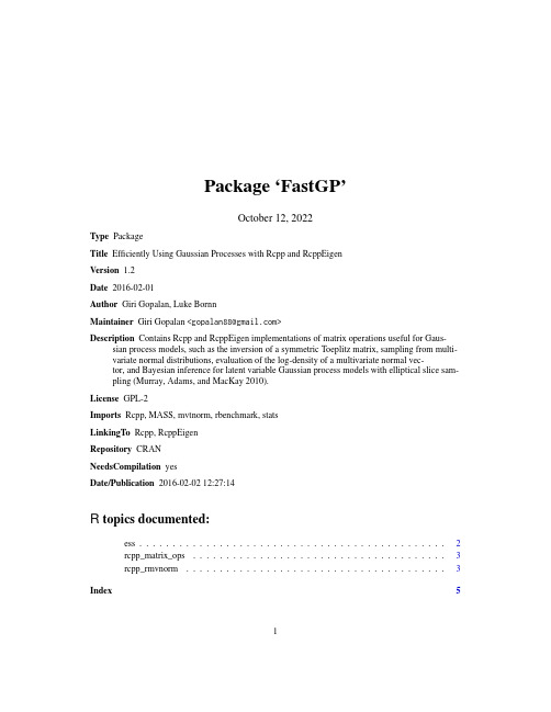
Package‘FastGP’October12,2022Type PackageTitle Efficiently Using Gaussian Processes with Rcpp and RcppEigenVersion1.2Date2016-02-01Author Giri Gopalan,Luke BornnMaintainer Giri Gopalan<*******************>Description Contains Rcpp and RcppEigen implementations of matrix operations useful for Gaus-sian process models,such as the inversion of a symmetric Toeplitz matrix,sampling from multi-variate normal distributions,evaluation of the log-density of a multivariate normal vec-tor,and Bayesian inference for latent variable Gaussian process models with elliptical slice sam-pling(Murray,Adams,and MacKay2010).License GPL-2Imports Rcpp,MASS,mvtnorm,rbenchmark,statsLinkingTo Rcpp,RcppEigenRepository CRANNeedsCompilation yesDate/Publication2016-02-0212:27:14R topics documented:ess (2)rcpp_matrix_ops (3)rcpp_rmvnorm (3)Index512ess ess Sampling from a Bayesian model with a multivariate normal prior dis-tributionDescriptionThis function uses elliptical slice sampling to sample from a Bayesian model in which the prior is multivariate normal(JMLR Murray,Adams,and MacKay2010)Usageess(log.lik,Y,Sig,N_mcmc,burn_in,N,flag)Argumentslog.lik Log-lik function in model which is assumed to take two arguments:thefirst contains the parameters/latent variables and the second the observed data Y Y Observed data.Sig Covariance matrix associated with the prior distribution on the parameters/latent variable vector.N_mcmc Number of desired mcmc samples.burn_in Number of burn-in iterations.N Dimensionality of parameter/latent variable vector.flag Set to TRUE for MASS implementation of mvrnorm(which may be more stable but slow),FALSE for FastGP implementation of rcpp_rmvnorm(which is fasterbut less stable)Author(s)Giri Gopalan*******************Examples#See demo/FastGPdemo.r.rcpp_matrix_ops3 rcpp_matrix_ops Matrix Operations Using Rcpp and RcppEigenDescriptionPerforms useful matrix operations using Rcpp and RcppEigen.Usagercppeigen_invert_matrix(A)rcppeigen_get_det(A)rcppeigen_get_chol(A)rcppeigen_get_chol_stable(A)rcppeigen_get_chol_diag(A)tinv(A)ArgumentsA Matrix to perform operation on.DetailsFunctions with"rcppeigen"directly call RcppEigen implementations of the associated functions;rcppeigen_get_chol_stable retrieves L and rcppeigen_get_chol_diag(A)retrieves D in A=LDL^T form,whereas rcppeigen_get_chol(A)retrieves L in A=LL^T form.Thanks to Jared Knowles who pointed out that the former variant is more stable(with a potential speed trade-off)and has found it useful for his package merTools.tinv inverts a symmetric Toeplitz matrix using methods from Trench and Durbin from"Matrix Computations"by Golub and Van Loan using Rcpp.Author(s)*******************Examples#See demo/FastGPdemo.Rrcpp_rmvnorm Multivariate Normal Sampling and Log-Density EvaluationDescriptionThese functions allow for the sampling of and evaluation of the log-density of a multivariate normal vector.4rcpp_rmvnormUsagercpp_log_dmvnorm(S,mu,x,istoep)rcpp_rmvnorm(n,S,mu)rcpp_rmvnorm_stable(n,S,mu)ArgumentsS Covariance matrix of associated multivariate normal.n Number of(independent)samples to generate.mu Mean vector.x Vector of observations to evaluate the log-density of.istoep set this to TRUE if S is Toeplitz.Author(s)Giri Gopalan*******************Examples#See demo/FastGPdemo.RIndexdurbin(rcpp_matrix_ops),3ess,2rcpp_distance(rcpp_matrix_ops),3rcpp_log_dmvnorm(rcpp_rmvnorm),3rcpp_matrix_ops,3rcpp_rmvnorm,3rcpp_rmvnorm_stable(rcpp_rmvnorm),3 rcppeigen_get_chol(rcpp_matrix_ops),3 rcppeigen_get_chol_diag(rcpp_matrix_ops),3rcppeigen_get_chol_stable(rcpp_matrix_ops),3rcppeigen_get_det(rcpp_matrix_ops),3 rcppeigen_get_diag(rcpp_matrix_ops),3 rcppeigen_invert_matrix(rcpp_matrix_ops),3tinv(rcpp_matrix_ops),3trench(rcpp_matrix_ops),35。
OPS原理及其实现方式
• 实验结果:无显著差别(Bland-Altman analysis)
• OPS 验证: 动物实验
• 实验模型:老鼠皮瓣和提睾肌;仓鼠背侧皮肤褶: • 实验内容: OPS vs. IVM 毛细血管密度(FCD);毛细血管直径 • 实验结果:良好一致性 • 实验模型:仓鼠背侧皮肤褶: • 实验内容: OPS vs. IVM 血液稀释条件下毛细血管密度(FCD);毛细血管直径 • 实验结果:良好一致性
• Gold standard :活体显微镜被公认为微循环参 数的金标准。(动物实验) • 图像清晰度高 •荧光染料对人体有毒性,无法做人体实验 •体积庞大,不适合作为临床使用 • 目前人体微循环在显微尺度下的唯一方法 • 局限于体表(皮肤甲襞、眼球结膜) • 对温度和血管收缩剂敏感 • 对发热病人的观测不准确:critically ill patients • 图像清晰度不好 • 临床使用: • 严重脓毒症患者皮肤和肌肉的微循环监测 • 在败血症/手术病人使用肾上腺素治疗时胃 和空肠黏膜血流量监测 • 测量区域平均值,无法体现毛细血管间的异性 (实验研究的主要特征之一)
可对人体微循环 在显微尺度下观察
可测量血流速度
临床应用
disadvantage
注射荧光染料, 局限于皮肤甲襞、 无法对人体使用 眼球结膜对温度和血 管收缩剂敏感 测量区域平均值 体积过大,不 对发热病人的观 适合临床应用 测不准确
• 微循环监测方式现状: Critical role vs. Limited approach
• OPS 验证: 动物实验
这些验证试验都是基于IVM和OPS的对比。一般认为 IVM是微循环参数的金标准( 目前对微循环的认识主要来 自动物的活体显微镜实验。 )。
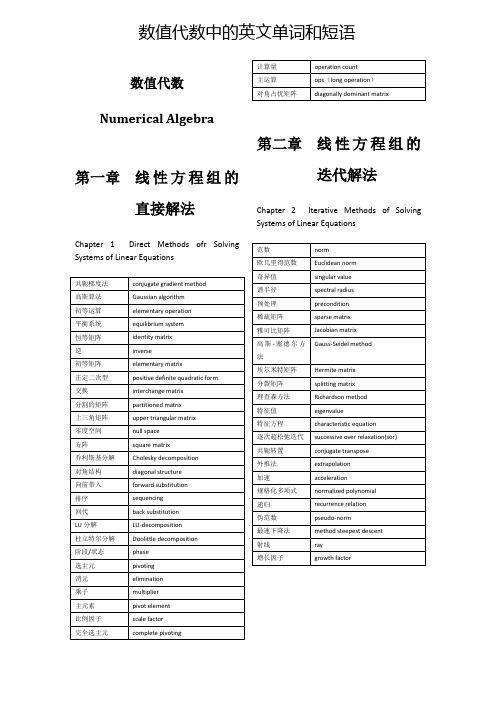
数值代数中的英文单词和短语
acceleration
规格化多项式
normalized polynomial
递归
recurrence relation
伪范数
pseudo-norm
最速下降法
method steepest descent
射线
ray
增长因子
growth factor
第三章
Chapter 3Solutions of Nonlinear Equation(s)
特征向量
eigenvector
幂法
power method
反幂法
inverse power method
埃特金加速
Aitken acceleration
差分
difference
酉相似
unitary similarity
降阶
reduction of order
谱
spectrum
最小二乘
lest-square
成分/分量
component
毕达哥拉斯法则 equation
格拉姆-施密特过程
Gram –Schmitt process
豪斯霍尔德变换
Householder transformation
奇异值分解
singular value decomposition
splitting matrix
理查森方法
Richardson method
特征值
eigenvalue
特征方程
characteristic equation
逐次超松弛迭代
successive over relaxation(sor)
共轭转置
conjugate transpose
触摸IC TTP226

DO
去除抖动的 I0 去除抖动的 I1 去除抖动的 I2 去除抖动的 I3 去除抖动的 I4 去除抖动的 I5 去除抖动的 I6 去除抖动的 I7 去除抖动的 I0 去除抖动的 I1
09’/08/31
Page 7 of 15
Ver :2.2
Preliminary
串行模式 RST、CK 和 DO 的时序 (图中为最小值)
AHL
25
OPS0
09’/08/31
Page 1 of 15
Ver :2.2
Preliminary
直接(DIRECT)模式框图:
OSC2 TOPAD I0 I1 I2 I3 I4 I5 I6 I7 OSC1 TEST
SLSE0 SLSE1 SLSE2 SLSE3 SLSE4 SLSE5
输入 扫描& 转换
17us
DV RST CK DO
62us
62us
62us
D0
D1
D2
D3
D4
D5
TTP226 TonTouchTM
D6
D7
D0
D1
5. 有效KEY触发,输出持续时间.
OPT1 1 1 0 0
OPT0 1 0 1 0
输出持续时间 无穷大 (关闭输出定时)
10 秒后复位系统 30 秒后复位系统 60 秒后复位系统
SCN0 为矩阵模式下的第一个扫描(scanning)管脚
29
Q1
(SCN1)
I/O Q1 为直接模式下的输出管脚
SCN1 为矩阵模式下的第二个扫描(scanning)管脚
30
NC
31
OPST
I-PH 选择灵敏度的基阶(base step)
python confusion matrix 结果解读
python confusion matrix 结果解读全文共四篇示例,供读者参考第一篇示例:混淆矩阵是机器学习中常用的评估模型性能的工具之一,特别是对于分类问题而言。
在Python中,我们可以使用各种库和工具来创建和解释混淆矩阵,比如scikit-learn库等。
混淆矩阵是一个二维矩阵,它展示了模型在测试数据集上的预测结果与真实标签之间的关系。
在混淆矩阵中,行代表真实标签,列代表预测标签,每个元素表示对应标签的样本数。
在混淆矩阵中,我们通常可以看到四个重要的指标,它们是真正例(True Positive,TP)、假正例(False Positive,FP)、真负例(True Negative,TN)和假负例(False Negative,FN)。
TP表示模型正确预测为正例的样本数,FP代表模型错误预测为正例的样本数,TN表示模型正确预测为负例的样本数,FN代表模型错误预测为负例的样本数。
通过这些指标,我们可以计算出模型的准确率、召回率、精确率和F1分数等评估指标。
准确率表示模型正确预测样本的比例,召回率表示模型正确预测正例的比例,精确率表示模型预测为正例的样本中真正为正例的比例,F1分数是综合考虑了召回率和精确率的一个评价指标。
在解读混淆矩阵的结果时,我们可以根据需要选择不同的指标来评估模型的性能。
如果我们更关注模型的准确率,那么我们可以查看混淆矩阵中的对角线元素的比例;如果我们更关注模型的召回率,那么我们可以查看TP/(TP+FN);如果我们更关注模型的精确率,那么我们可以查看TP/(TP+FP)。
通过对混淆矩阵进行可视化,我们还可以更直观地了解模型的性能。
比如我们可以使用热力图来展示混淆矩阵,不同颜色的方块代表不同数量的样本数量,从而更清晰地看到模型的预测结果。
混淆矩阵是一个非常有用的工具,可以帮助我们评估机器学习模型的性能。
通过对混淆矩阵的解读,我们可以更全面地了解模型在不同指标下的表现,从而更好地优化和改进模型。
rust矩阵运算 -回复
rust矩阵运算-回复Rust矩阵运算: 优化性能与简化代码的完美结合引言:矩阵运算在科学计算和数据处理领域中起着重要的作用。
无论是进行向量或矩阵相乘、转置、求逆矩阵,还是求解线性方程组,矩阵运算是不可或缺的工具。
Rust作为一种高性能、系统级别的编程语言,提供了丰富的特性和工具,使得进行矩阵运算变得更加高效和易于实现。
本文将重点介绍Rust中矩阵运算的相关库和技术。
我们将一步步讨论如何从零开始构建一个简单的矩阵库,并通过不断优化性能和简化代码,实现一个高效、易用的矩阵运算库。
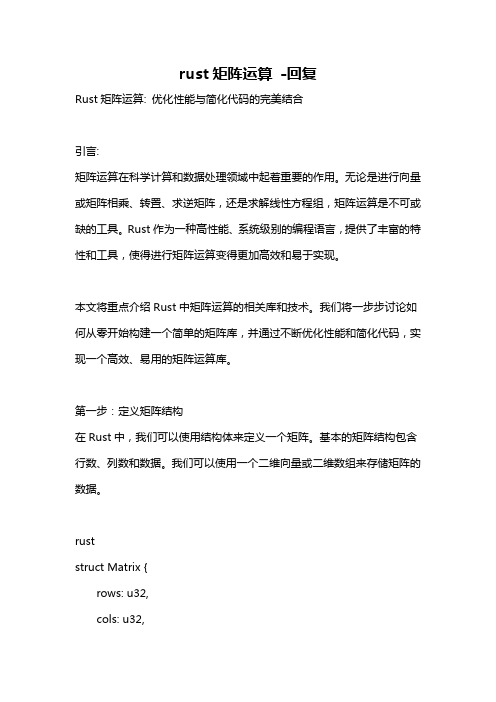
第一步:定义矩阵结构在Rust中,我们可以使用结构体来定义一个矩阵。
基本的矩阵结构包含行数、列数和数据。
我们可以使用一个二维向量或二维数组来存储矩阵的数据。
ruststruct Matrix {rows: u32,cols: u32,data: Vec<Vec<f64>>,}第二步:实现基本的矩阵运算现在,我们可以着手实现一些基本的矩阵运算,比如相加和相乘。
通过实现运算符重载,我们可以使用简洁的代码来执行这些运算。
rustuse std::ops::{Add, Mul};impl Add for Matrix {type Output = Matrix;fn add(self, other: Matrix) -> Matrix {检查矩阵尺寸是否兼容assert_eq!(self.rows, other.rows);assert_eq!(self.cols, other.cols);创建一个新的矩阵let mut result = Matrix::new(self.rows, self.cols);执行加法运算for i in 0..self.rows {for j in 0..self.cols {result.data[i][j] = self.data[i][j] + other.data[i][j];}}result}}impl Mul for Matrix {type Output = Matrix;fn mul(self, other: Matrix) -> Matrix {检查矩阵尺寸是否兼容assert_eq!(self.cols, other.rows);创建一个新的矩阵let mut result = Matrix::new(self.rows, other.cols);执行乘法运算for i in 0..self.rows {for j in 0..other.cols {for k in 0..self.cols {result.data[i][j] += self.data[i][k] *other.data[k][j];}}}result}}通过添加其他运算符的实现,比如减法和除法,我们可以完成更多的矩阵运算。
rust矩阵运算 -回复
rust矩阵运算-回复Rust矩阵运算: 从基础到高级在计算机科学和数学领域,矩阵是一种非常重要的数据结构。
它们能够用于表示和处理线性关系,并在各种应用中发挥关键作用,包括图形处理、机器学习、金融建模等。
Rust是一种强大的系统编程语言,具有内存安全和高性能的特点。
本文将介绍如何使用Rust进行矩阵运算,从基础到高级,逐步引导您完成。
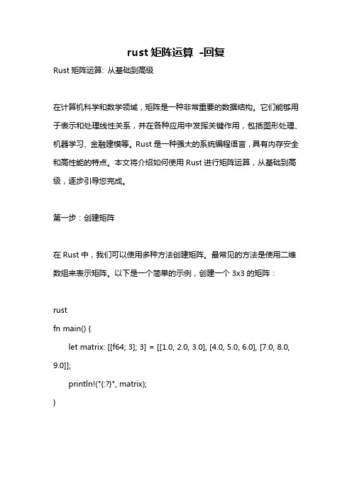
第一步:创建矩阵在Rust中,我们可以使用多种方法创建矩阵。
最常见的方法是使用二维数组来表示矩阵。
以下是一个简单的示例,创建一个3x3的矩阵:rustfn main() {let matrix: [[f64; 3]; 3] = [[1.0, 2.0, 3.0], [4.0, 5.0, 6.0], [7.0, 8.0, 9.0]];println!("{:?}", matrix);}在上述示例中,我们定义了一个名为`matrix`的常量,它是一个3x3的矩阵,每个元素都是`f64`类型(64位浮点数)。
我们使用嵌套的数组语法来表示矩阵的行和列。
第二步:访问矩阵元素要访问矩阵中的特定元素,我们可以使用索引操作符`[行][列]`。
以下是一个示例:rustfn main() {let matrix: [[f64; 3]; 3] = [[1.0, 2.0, 3.0], [4.0, 5.0, 6.0], [7.0, 8.0, 9.0]];println!("matrix[0][0]: {}", matrix[0][0]); 输出矩阵第一行第一列的元素println!("matrix[1][2]: {}", matrix[1][2]); 输出矩阵第二行第三列的元素}在上述示例中,我们使用索引操作符`[行][列]`访问矩阵中的元素。
注意索引从0开始。
第三步:矩阵相加在Rust中,要计算两个矩阵的和,我们需要定义一个`Matrix`结构体,并实现`Add` trait。
keras ops函数

keras ops函数
Keras是一个开源的深度学习框架,它提供了一系列的操作函
数(ops functions)来构建神经网络模型。
这些操作函数包括了各
种神经网络层、激活函数、优化器等,下面我将从不同角度来介绍
一些常用的Keras操作函数。
首先,Keras提供了丰富的神经网络层,如Dense(全连接层)、Conv2D(二维卷积层)、LSTM(长短期记忆网络)等。
这些层可以
通过简单的方式来构建深度神经网络模型,使得模型的构建变得非
常方便。
其次,Keras还提供了多种激活函数,如ReLU(线性整流函数)、Sigmoid(S形函数)、tanh(双曲正切函数)等。
这些激活
函数可以帮助神经网络引入非线性,从而提升模型的表达能力。
此外,Keras还包含了各种优化器,如SGD(随机梯度下降)、Adam(自适应矩估计优化算法)、RMSprop(均方根传播)等。
这些
优化器可以帮助神经网络更快地收敛,提高训练效率。
除了以上提到的内容,Keras还提供了一些辅助函数,如
Dropout(随机失活)、BatchNormalization(批标准化)等,这些函数可以帮助提升模型的泛化能力和训练稳定性。
总的来说,Keras的操作函数涵盖了神经网络模型构建的方方面面,使得用户能够更加便捷地构建、训练和部署深度学习模型。
希望这些信息能够帮助你更好地理解Keras的操作函数。
python 仿射变换矩阵与点云框matrix矩阵格式计算

python 仿射变换矩阵与点云框matrix矩阵格式计算摘要:1.仿射变换简介2.仿射变换矩阵及其计算方法3.点云框matrix矩阵格式计算4.Python实现仿射变换5.应用实例:图像处理和三维重建正文:一、仿射变换简介仿射变换是一种线性变换,它包括平移、缩放、旋转等基本变换。
在二维空间中,仿射变换可以描述为:Affine transformation: (x", y") = (Ax + b, By + c)其中,(x", y")表示目标图像中的坐标,(x, y)表示原图像中的坐标,A、B、a、b、c为变换参数。
二、仿射变换矩阵及其计算方法仿射变换矩阵包含6个未知数,需要至少6个方程才能解出所有的未知数。
一般情况下,我们可以通过已知的3对坐标(至少6个点)来计算仿射矩阵。
计算方法如下:1.选取3对坐标(至少6个点)作为已知条件。
2.列出方程组,求解变换矩阵。
三、点云框matrix矩阵格式计算点云框matrix矩阵格式计算是将点云数据转换为特定格式的过程。
在Python中,我们可以使用OpenCV库来实现这一功能。
四、Python实现仿射变换1.安装OpenCV库:在使用OpenCV之前,需要先安装Python的OpenCV库。
可以使用以下命令进行安装:```pip install opencv-python```2.使用OpenCV实现仿射变换:```pythonimport cv2# 读取图像img = cv2.imread("input.jpg")# 获取图像的宽度和高度h, w = img.shape[:2]# 选取3对坐标(至少6个点)src_pts = np.float32([[50,50], [200,50], [50,200]])dst_pts = np.float32([[10,100], [200,50], [100,250]])# 计算仿射矩阵M = cv2.getAffineTransform(src_pts, dst_pts)# 进行仿射变换dst = cv2.warpAffine(img, M, (w, h))# 显示结果cv2.imshow("Result", dst)cv2.waitKey(0)cv2.destroyAllWindows()```五、应用实例:图像处理和三维重建1.图像处理:在图像处理领域,仿射变换常用于图像拼接、图像校正、图像识别等任务。
confusion_matrix参数说明
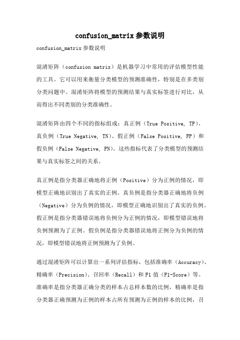
confusion_matrix参数说明confusion_matrix参数说明混淆矩阵(confusion matrix)是机器学习中常用的评估模型性能的工具。
它可以用来衡量分类模型的预测准确性,特别是在多类别分类问题中。
混淆矩阵将模型的预测结果与真实标签进行对比,从而得出不同类别的分类准确性。
混淆矩阵由四个不同的指标组成:真正例(True Positive, TP)、真负例(True Negative, TN)、假正例(False Positive, FP)和假负例(False Negative, FN)。
这些指标代表了分类模型的预测结果与真实标签之间的关系。
真正例是指分类器正确地将正例(Positive)分为正例的情况,即模型正确地识别出了真实的正例。
真负例是指分类器正确地将负例(Negative)分为负例的情况,即模型正确地识别出了真实的负例。
假正例是指分类器错误地将负例分为正例的情况,即模型错误地将负例预测为了正例。
假负例是指分类器错误地将正例分为负例的情况,即模型错误地将正例预测为了负例。
通过混淆矩阵可以计算出一系列评估指标,包括准确率(Accuracy)、精确率(Precision)、召回率(Recall)和F1值(F1-Score)等。
准确率是指分类器正确分类的样本占总样本数的比例,精确率是指分类器正确预测为正例的样本占所有预测为正例的样本的比例,召回率是指分类器正确预测为正例的样本占所有真实正例的样本的比例,F1值综合了精确率和召回率,是一个综合评价指标。
混淆矩阵的使用有助于了解分类模型在不同类别上的分类效果。
通过观察混淆矩阵的各个指标,可以判断模型在不同类别上的表现情况,进而对模型进行调整和改进。
例如,如果模型在某个类别上的召回率较低,可以通过调整模型的参数或增加该类别的训练样本来提升模型在该类别上的分类性能。
在实际应用中,混淆矩阵经常与其他评估指标一起使用。
例如,通过对不同类别的混淆矩阵进行加权平均,可以得到一个更全面的评估指标,如平均准确率(Average Accuracy)或平均F1值(Average F1-Score)。
稀疏矩阵(sparsematrix)

在数值分析中,稀疏矩阵(Sparse matrix),是其元素大部分为零的矩阵。反之,如果大部分元素都非零,则这个矩阵是稠密的。在科学与 工程领域中求解线性模型时经常出现大型的稀疏矩阵。 在使用计算机存储和操作稀疏矩阵时,经常需要修改标准算法以利用矩阵的稀疏结构。由于其自身的稀疏特性,通过压缩可以大大节省稀疏 矩阵的内存代价。更为重要的是,由于过大的尺寸,标准的算法经常无法操作这些稀疏矩阵。
版权声明:本文为博主原创文章,未经博主允许不得转载。