S. Kernel Basis Pursuit
压缩感知去噪代码
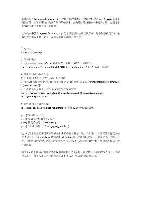
压缩感知(Compressed Sensing)是一种信号处理技术,它允许我们以远低于Nyquist采样率测量信号,从而显著减少数据存储和传输需求。
去噪是信号处理的一个重要步骤,它通过消除或减少噪声来提高信号的质量。
以下是一个使用Python和NumPy库的简单压缩感知去噪代码示例。
这个例子使用了L1最小化方法进行去噪,它是一种常见的压缩感知去噪方法。
```pythonimport numpy as np# 信号和噪声x = np.random.randn(100) # 随机生成一个包含100个元素的信号s = np.dot(np.random.randn(90), x[90:100]) + np.random.randn(10) # 添加一些噪声# 使用压缩感知恢复信号# 这里我们使用L1最小化方法进行去噪# 注意:在实际应用中,你可能需要使用更复杂的算法,如OMP(Orthogonal Matching Pursuit)或Basis Pursuit等# 下面仅是为了说明,并不是压缩感知的精确实现Rx = np.dot(np.linalg.inv(np.linalg.svd(np.random.randn(5))), np.random.randn(5))rec_signal = np.dot(Rx, s)# 对恢复的信号进行去噪rec_signal_denoised = np.abs(rec_signal) # 使用L1最小化方法去噪print("原始信号:", x)print("添加噪声后的信号:", s)print("恢复的信号:", rec_signal)print("去噪后的信号:", rec_signal_denoised)```这个代码示例仅用于说明压缩感知和去噪的基本概念。
在实际应用中,你需要使用更复杂的算法和工具,如scikit-learn库中的L1Minimizer类,或者使用深度学习的方法进行去噪。
匹配追踪算法和基追踪

匹配追踪算法和基追踪英文回答:Matching Pursuit (MP) Algorithm and Basis Pursuit (BP)。
Matching pursuit (MP) and basis pursuit (BP) are two closely related algorithms used for signal reconstruction and decomposition. They are iterative greedy algorithmsthat aim to find the best representation of a signal as a linear combination of basis elements or atoms.Matching Pursuit Algorithm.MP is an iterative algorithm that starts with aninitial guess of the signal representation and then iteratively adds basis elements to the representation until a stopping criterion is met. At each iteration, MP selects the basis element that best matches the residual of the signal (the difference between the current representation and the original signal). The selected basis element isthen added to the representation, and the residual is updated.Basis Pursuit Algorithm.BP is a variation of MP that uses a regularization term to penalize the size of the representation. This regularization term helps to prevent overfitting and produces a more stable representation of the signal. BP solves a constrained optimization problem to find the representation that minimizes the sum of the squared error between the representation and the original signal and the regularization term.Applications.MP and BP are widely used in signal processing and machine learning applications, including:Signal denoising.Image compression.Feature extraction.Anomaly detection.Speech recognition.Advantages and Disadvantages.Advantages:Simple and computationally efficient.Can produce sparse representations.Can be used with a variety of basis sets.Disadvantages:Can be sensitive to noise.Does not always converge to the optimal solution.Can be slow for large signals.中文回答:匹配追踪算法和基追踪算法。
基于SBL算法的大间隔非等间距阵DOA估计技术
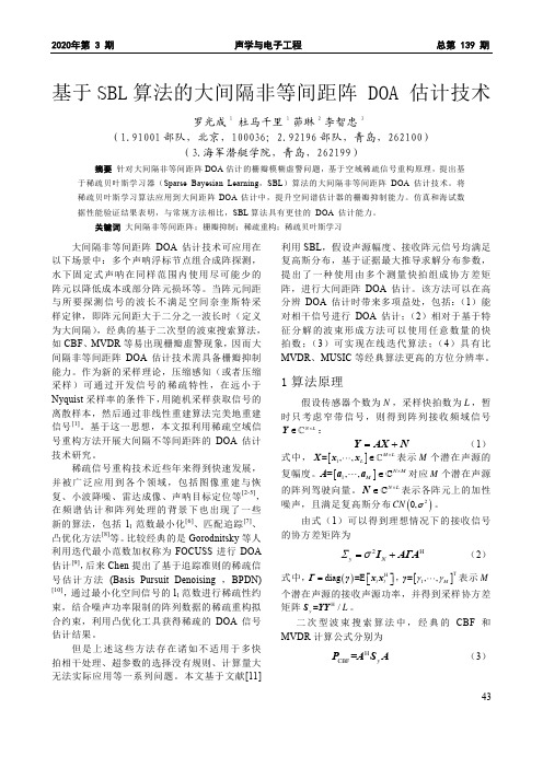
2020年第 3 期 声学与电子工程 总第 139 期基于SBL算法的大间隔非等间距阵 DOA 估计技术罗光成1 杜马千里 1 茆琳 2 李智忠3(1.91001部队,北京,100036;2.92196部队,青岛,262100)(3.海军潜艇学院,青岛,262199)摘要 针对大间隔非等间距阵DOA估计的栅瓣模糊虚警问题,基于空域稀疏信号重构原理,提出基于稀疏贝叶斯学习器(Sparse Bayesian Learning,SBL)算法的大间隔非等间距阵 DOA 估计技术。
将稀疏贝叶斯学习算法应用到大间距阵DOA估计中,提升空间谱估计器的栅瓣抑制能力。
仿真和海试数据性能验证结果表明,与常规方法相比,SBL算法具有更佳的 DOA 估计能力。
关键词大间隔非等间距阵;栅瓣抑制;稀疏重构;稀疏贝叶斯学习大间隔非等间距阵DOA估计技术可应用在以下场景中:多个声呐浮标节点组合成阵探测,水下固定式声呐在同样范围内使用尽可能少的阵元以降低成本或部分阵元损坏等。
当阵元间距与所要探测信号的波长不满足空间奈奎斯特采样定律,即阵元间距大于二分之一波长时(定义为大间隔),经典的基于二次型的波束搜索算法,如CBF、MVDR等易出现栅瓣虚警现象,因而大间隔非等间距阵DOA估计技术需具备栅瓣抑制能力。
作为新的采样理论,压缩感知(或者压缩采样)可通过开发信号的稀疏特性,在远小于Nyquist采样率的条件下,用随机采样获取信号的离散样本,然后通过非线性重建算法完美地重建信号[1]。
基于这一思想,本文拟利用稀疏空域信号重构方法开展大间隔不等间距阵的DOA估计技术研究。
稀疏信号重构技术近些年来得到快速发展,并被广泛应用到各个领域,包括图像重建与恢复、小波降噪、雷达成像、声呐目标定位等[2-5],在频谱估计和阵列处理的背景下也出现了一些新的算法,包括l1范数最小化[6]、匹配追踪[7]、凸优化方法[8]等。
比较经典的是Gorodnitsky等人利用迭代最小范数加权称为FOCUSS进行DOA 估计[9],后来Chen提出了基于追踪准则的稀疏信号估计方法 (Basis Pursuit Denoising ,BPDN) [10],通过最小化空间信号的l1范数进行稀疏性约束,结合噪声功率限制的阵列数据的稀疏重构拟合约束,利用凸优化工具获得稀疏的DOA信号估计结果。
压缩感知的重构算法
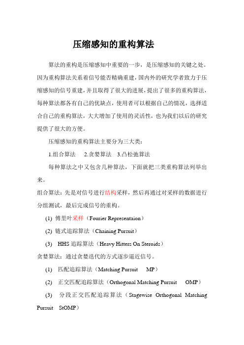
压缩感知的重构算法算法的重构是压缩感知中重要的一步,是压缩感知的关键之处。
因为重构算法关系着信号能否精确重建,国内外的研究学者致力于压缩感知的信号重建,并且取得了很大的进展,提出了很多的重构算法,每种算法都各有自己的优缺点,使用者可以根据自己的情况,选择适合自己的重构算法,大大增加了使用的灵活性,也为我们以后的研究提供了很大的方便。
压缩感知的重构算法主要分为三大类:1.组合算法2.贪婪算法3.凸松弛算法每种算法之中又包含几种算法,下面就把三类重构算法列举出来。
组合算法:先是对信号进行结构采样,然后再通过对采样的数据进行分组测试,最后完成信号的重构。
(1) 傅里叶采样(Fourier Representaion)(2) 链式追踪算法(Chaining Pursuit)(3) HHS追踪算法(Heavy Hitters On Steroids)贪婪算法:通过贪婪迭代的方式逐步逼近信号。
(1) 匹配追踪算法(Matching Pursuit MP)(2) 正交匹配追踪算法(Orthogonal Matching Pursuit OMP)(3) 分段正交匹配追踪算法(Stagewise Orthogonal Matching Pursuit StOMP)(4) 正则化正交匹配追踪算法(Regularized Orthogonal Matching Pursuit ROMP)(5) 稀疏自适应匹配追踪算法(Sparisty Adaptive Matching Pursuit SAMP)凸松弛算法:(1) 基追踪算法(Basis Pursuit BP)(2) 最小全变差算法(Total Variation TV)(3) 内点法(Interior-point Method)(4) 梯度投影算法(Gradient Projection)(5) 凸集交替投影算法(Projections Onto Convex Sets POCS)算法较多,但是并不是每一种算法都能够得到很好的应用,三类算法各有优缺点,组合算法需要观测的样本数目比较多但运算的效率最高,凸松弛算法计算量大但是需要观测的数量少重构的时候精度高,贪婪迭代算法对计算量和精度的要求居中,也是三种重构算法中应用最大的一种。
强化学习的马尔可夫决策过程与值函数

强化学习的马尔可夫决策过程与值函数强化学习是一种机器学习领域中的方法,旨在使机器能够通过与环境互动来学习最佳行动策略。
马尔可夫决策过程(MDP)和值函数是强化学习中的两个核心概念。
在本文中,我们将详细介绍马尔可夫决策过程和值函数,并讨论它们在强化学习中的作用。
一、马尔可夫决策过程(MDP)马尔可夫决策过程是强化学习中用于建模决策问题的数学框架。
它是一种序列决策问题,其中智能体根据环境的状态进行决策,并接收激励信号来调整自己的行为。
MDP主要由以下几个要素组成:1. 状态空间(State Space):状态空间是指环境可能处于的所有状态的集合。
每个状态都代表了环境的一个特定配置。
在MDP中,状态可以是离散的(如棋盘上的位置)或连续的(如机器人的位置和速度)。
2. 动作空间(Action Space):动作空间是指智能体可以选择的所有可能动作的集合。
每个动作都会导致环境从一个状态转移到另一个状态。
3. 转移概率(Transition Probability):转移概率定义了在给定当前状态和动作的情况下,环境转移到下一个状态的概率。
这可以用一个转移函数来表示,即P(s'|s, a),其中s'代表下一个状态,s代表当前状态,a代表当前动作。
4. 奖励函数(Reward Function):奖励函数定义了智能体在不同状态和采取不同动作时获得的即时奖励。
奖励可以是正值、负值或零,用来评估智能体的行为。
5. 折扣因子(Discount Factor):折扣因子(通常用γ表示)被引入到MDP中,用于表示未来奖励的重要性相对于即时奖励的衰减程度。
如果折扣因子接近于0,智能体将更关注即时奖励;如果折扣因子接近于1,智能体将更关注未来的奖励。
基于上述要素,马尔可夫决策过程可以通过一个状态-动作-奖励的序列表示,即{<s_0, a_0, r_0>, <s_1, a_1, r_1>, <s_2, a_2,r_2>, ...}。
《Kernel Sparse Representation》中文翻译
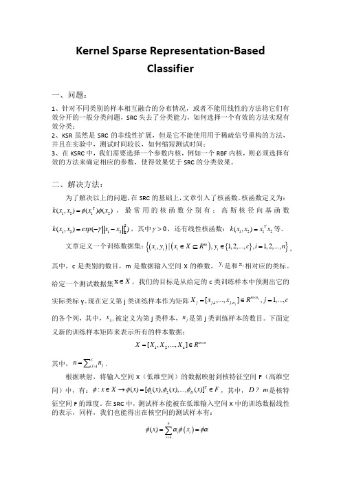
Kernel Sparse Representation-BasedClassifier一、问题:1、针对不同类别的样本相互融合的分布情况,或者不能用线性的方法将它们有效分开的一般分类问题,SRC 失去了分类能力,如何选择一个有效的方法实现有效分类;2、KSR 虽然是SRC 的非线性扩展,但是它不能使用用于稀疏信号重构的方法,并且在实验中,测试时间较长,如何缩短测试时间;3、在KSRC 中,我们需要选择一个参数内核,例如一个RBF 内核,则必须选择有效的方法来确定相应的参数,使得效果优于SRC 的分类效果。
二、解决方法:为了解决以上的问题,在SRC 的基础上,文章引入了核函数。
核函数定义为: 1212(,)()()T k x x x x φφ=。
最常用的核函数分别有:高斯核径向基函数212122(,)()k x x exp x x γ=--,其中0γ>,还有线性核函数:1212(,)T k x x x x =等。
文章定义一个训练数据集:()(){}{},|,1,2,...,,1,2,...,m i i i i x y x X R y c i n ∈⊆∈=,其中,c 是类别的数目,m 是数据输入空间X 的维数,i y 是和i x 相对应的类标。
给定一个测试数据集x X ∈,我们的目标是从给定的c 类训练样本中预测出它的实际类标y 。
现在定义第j 类训练样本作为矩阵,1,[,...,],1,...,j j m n j j j n X x x R j c ⨯=∈=的各个列,其中,,j i x 被定义为第j 类样本,j n 是第j 类训练样本的数目。
下面定义新的训练样本矩阵来表示所有的样本数据:12c [,,...,]m n X X X X R ⨯=∈其中,1c j j n n ==∑.根据映射,将输入空间X (低维空间)的数据映射到核特征空间F (高维空间)中,有:12:()[(),(),...,()]T D x X x x x x F φφφφφ∈→=∈,其中,D m 是核特征空间F 的维度。
基于稀疏重建的信号DOA估计
基于稀疏重建的信号DOA估计任肖丽;王骥;万群【摘要】从稀疏信号重建角度提出了一种改进的波达方向(DOA)估计方法。
由于最小冗余线阵(MRLA)能以较少的阵元数获得较大的阵列孔径,将MRLA与ℓ1-SVD方法相结合估计信号的DOA。
仿真结果表明,经多次实验验证,所提方法是有效的,相比ℓ1-SVD方法可以估计出更多信源的DOA,并且可以用较少的阵元数估计更多的信源DOA,具有信源过载能力。
%This paper proposes a modified Direction of Arrival(DOA)estimation method based on Minimum Redundancy Linear Array(MRLA)from the sparse signal reconstruction perspective. According to the structure feature of MRLA that obtaining larger antenna aperture through a smaller number of array sensors, MRLA is combined with ℓ1-SVD method to estimate signal DOAs. Simulations demonstrate that the proposed method is effective, and compared with ℓ1-SVD meth-od it can estimate more DOAs of signal source, and it is capable of estimating more DOAs with fewer antenna elements.【期刊名称】《计算机工程与应用》【年(卷),期】2015(000)001【总页数】6页(P195-199,217)【关键词】波达方向(DOA);稀疏信号重建;最小冗余线阵(MRLA);ℓ1-SVD【作者】任肖丽;王骥;万群【作者单位】广东海洋大学信息学院,广东湛江 524088;广东海洋大学信息学院,广东湛江 524088;电子科技大学电子工程学院,成都 611731【正文语种】中文【中图分类】TN911.71 引言源定位是信号处理领域的主要目的之一,利用传感器阵列可以将其转换成DOA估计。
高斯朴素贝叶斯训练集精确度的英语
高斯朴素贝叶斯训练集精确度的英语Gaussian Naive Bayes (GNB) is a popular machine learning algorithm used for classification tasks. It is particularly well-suited for text classification, spam filtering, and recommendation systems. However, like any other machine learning algorithm, GNB's performance heavily relies on the quality of the training data. In this essay, we will delve into the factors that affect the training set accuracy of Gaussian Naive Bayes and explore potential solutions to improve its performance.One of the key factors that influence the training set accuracy of GNB is the quality and quantity of the training data. In order for the algorithm to make accurate predictions, it needs to be trained on a diverse and representative dataset. If the training set is too small or biased, the model may not generalize well to new, unseen data. This can result in low training set accuracy and poor performance in real-world applications. Therefore, it is crucial to ensure that the training data is comprehensive and well-balanced across different classes.Another factor that can impact the training set accuracy of GNB is the presence of irrelevant or noisy features in the dataset. When the input features contain irrelevant information or noise, it can hinder the algorithm's ability to identify meaningful patterns and make accurate predictions. To address this issue, feature selection and feature engineering techniques can be employed to filter out irrelevant features and enhance the discriminative power of the model. Byselecting the most informative features and transforming them appropriately, we can improve the training set accuracy of GNB.Furthermore, the assumption of feature independence in Gaussian Naive Bayes can also affect its training set accuracy. Although the 'naive' assumption of feature independence simplifies the model and makes it computationally efficient, it may not hold true in real-world datasets where features are often correlated. When features are not independent, it can lead to biased probability estimates and suboptimal performance. To mitigate this issue, techniques such as feature extraction and dimensionality reduction can be employed to decorrelate the input features and improve the training set accuracy of GNB.In addition to the aforementioned factors, the choice of hyperparameters and model tuning can also impact the training set accuracy of GNB. Hyperparameters such as the smoothing parameter (alpha) and the covariance type in the Gaussian distribution can significantly influence the model's performance. Therefore, it is important to carefully tune these hyperparameters through cross-validation andgrid search to optimize the training set accuracy of GNB. By selecting the appropriate hyperparameters, we can ensure that the model is well-calibrated and achieves high accuracy on the training set.Despite the challenges and limitations associated with GNB, there are several strategies that can be employed to improve its training set accuracy. By curating a high-quality training dataset, performing feature selection and engineering, addressing feature independence assumptions, and tuning model hyperparameters, we can enhance the performance of GNB and achieve higher training set accuracy. Furthermore, it is important to continuously evaluate and validate the model on unseen data to ensure that it generalizes well and performs robustly in real-world scenarios. By addressing these factors and adopting best practices in model training and evaluation, we can maximize the training set accuracy of Gaussian Naive Bayes and unleash its full potential in various applications.。
Atomic Decomposition by Basis pursuit
SIAM R EVIEWc2001Society for Industrial and Applied Mathematics Vol.43,No.1,pp.129–159Atomic Decomposition by BasisPursuit ∗Scott Shaobing Chen †David L.Donoho ‡Michael A.Saunders §Abstract.The time-frequency and time-scale communities have recently developed a large number ofovercomplete waveform dictionaries—stationary wavelets,wavelet packets,cosine packets,chirplets,and warplets,to name a few.Decomposition into overcomplete systems is not unique,and several methods for decomposition have been proposed,including the method of frames (MOF),matching pursuit (MP),and,for special dictionaries,the best orthogonal basis (BOB).Basis pursuit (BP)is a principle for decomposing a signal into an “optimal”superpo-sition of dictionary elements,where optimal means having the smallest l 1norm of coef-ficients among all such decompositions.We give examples exhibiting several advantages over MOF,MP,and BOB,including better sparsity and superresolution.BP has interest-ing relations to ideas in areas as diverse as ill-posed problems,abstract harmonic analysis,total variation denoising,and multiscale edge denoising.BP in highly overcomplete dictionaries leads to large-scale optimization problems.With signals of length 8192and a wavelet packet dictionary,one gets an equivalent linear program of size 8192by 212,992.Such problems can be attacked successfully only because of recent advances in linear and quadratic programming by interior-point methods.We obtain reasonable success with a primal-dual logarithmic barrier method and conjugate-gradient solver.Key words.overcomplete signal representation,denoising,time-frequency analysis,time-scale anal-ysis, 1norm optimization,matching pursuit,wavelets,wavelet packets,cosine pack-ets,interior-point methods for linear programming,total variation denoising,multiscale edges,MATLAB code AMS subject classifications.94A12,65K05,65D15,41A45PII.S003614450037906X1.Introduction.Over the last several years,there has been an explosion of in-terest in alternatives to traditional signal representations.Instead of just represent-ing signals as superpositions of sinusoids (the traditional Fourier representation)we now have available alternate dictionaries—collections of parameterized waveforms—of which the wavelets dictionary is only the best known.Wavelets,steerable wavelets,segmented wavelets,Gabor dictionaries,multiscale Gabor dictionaries,wavelet pack-∗Publishedelectronically February 2,2001.This paper originally appeared in SIAM Journal onScientific Computing ,Volume 20,Number 1,1998,pages 33–61.This research was partially sup-ported by NSF grants DMS-92-09130,DMI-92-04208,and ECS-9707111,by the NASA Astrophysical Data Program,by ONR grant N00014-90-J1242,and by other sponsors./journals/sirev/43-1/37906.html†Renaissance Technologies,600Route 25A,East Setauket,NY 11733(schen@).‡Department of Statistics,Stanford University,Stanford,CA 94305(donoho@).§Department of Management Science and Engineering,Stanford University,Stanford,CA 94305(saunders@).129D o w n l o a d e d 08/09/14 t o 58.19.126.38. R e d i s t r i b u t i o n s u b j e c t t o S I A M l i c e n s e o r c o p y r i g h t ; s e e h t t p ://w w w .s i a m .o r g /j o u r n a l s /o j s a .p h p130S.S.CHEN,D.L.DONOHO,AND M.A.SAUNDERSets,cosine packets,chirplets,warplets,and a wide range of other dictionaries are now available.Each such dictionary D is a collection of waveforms (φγ)γ∈Γ,with γa parameter,and we envision a decomposition of a signal s ass =γ∈Γαγφγ,(1.1)or an approximate decomposition s =m i =1αγi φγi +R (m ),(1.2)where R (m )is a residual.Depending on the dictionary,such a representation de-composes the signal into pure tones (Fourier dictionary),bumps (wavelet dictionary),chirps (chirplet dictionary),etc.Most of the new dictionaries are overcomplete ,either because they start out that way or because we merge complete dictionaries,obtaining a new megadictionary con-sisting of several types of waveforms (e.g.,Fourier and wavelets dictionaries).The decomposition (1.1)is then nonunique,because some elements in the dictionary have representations in terms of other elements.1.1.Goals of Adaptive Representation.Nonuniqueness gives us the possibility of adaptation,i.e.,of choosing from among many representations one that is most suited to our purposes.We are motivated by the aim of achieving simultaneously the following goals .•Sparsity.We should obtain the sparsest possible representation of the object—the one with the fewest significant coefficients.•Superresolution.We should obtain a resolution of sparse objects that is much higher resolution than that possible with traditional nonadaptive approaches.An important constraint ,which is perhaps in conflict with both the goals,follows.•Speed.It should be possible to obtain a representation in order O (n )or O (n log(n ))time.1.2.Finding a Representation.Several methods have been proposed for obtain-ing signal representations in overcomplete dictionaries.These range from general approaches,like the method of frames (MOF)[9]and the method of matching pursuit (MP)[29],to clever schemes derived for specialized dictionaries,like the method of best orthogonal basis (BOB)[7].These methods are described briefly in section 2.3.In our view,these methods have both advantages and shortcomings.The principal emphasis of the proposers of these methods is on achieving sufficient computational speed.While the resulting methods are practical to apply to real data,we show below by computational examples that the methods,either quite generally or in important special cases,lack qualities of sparsity preservation and of stable superresolution.1.3.Basis Pursuit.Basis pursuit (BP)finds signal representations in overcom-plete dictionaries by convex optimization:it obtains the decomposition that minimizes the 1normof the coefficients occurring in the representation.Because of the nondif-ferentiability of the 1norm,this optimization principle leads to decompositions that can have very different properties fromthe MOF—in particular,they can be m uch sparser.Because it is based on global optimization,it can stably superresolve in ways that MP cannot.D o w n l o a d e d 08/09/14 t o 58.19.126.38. R e d i s t r i b u t i o n s u b j e c t t o S I A M l i c e n s e o r c o p y r i g h t ; s e e h t t p ://w w w .s i a m .o r g /j o u r n a l s /o j s a .p h pATOMIC DECOMPOSITION BY BASIS PURSUIT131BP can be used with noisy data by solving an optimization problem trading offa quadratic misfit measure with an 1normof coefficients.Examples show that it can stably suppress noise while preserving structure that is well expressed in the dictionary under consideration.BP is closely connected with linear programming.Recent advances in large-scale linear programming—associated with interior-point methods—can be applied to BP and can make it possible,with certain dictionaries,to nearly solve the BP optimization problem in nearly linear time.We have implemented primal-dual log barrier interior-point methods as part of a MATLAB [31]computing environment called Atomizer,which accepts a wide range of dictionaries.Instructions for Internet access to Atomizer are given in section 7.3.Experiments with standard time-frequency dictionaries indicate some of the potential benefits of BP.Experiments with some nonstandard dictionaries,like the stationary wavelet dictionary and the heaviside dictionary,indicate important connections between BP and methods like Mallat and Zhong’s [29]multiscale edge representation and Rudin,Osher,and Fatemi’s [35]total variation-based denoising methods.1.4.Contents.In section 2we establish vocabulary and notation for the rest of the article,describing a number of dictionaries and existing methods for overcomplete representation.In section 3we discuss the principle of BP and its relations to existing methods and to ideas in other fields.In section 4we discuss methodological issues associated with BP,in particular some of the interesting nonstandard ways it can be deployed.In section 5we describe BP denoising,a method for dealing with problem (1.2).In section 6we discuss recent advances in large-scale linear programming (LP)and resulting algorithms for BP.For reasons of space we refer the reader to [4]for a discussion of related work in statistics and analysis.2.Overcomplete Representations.Let s =(s t :0≤t <n )be a discrete-time signal of length n ;this may also be viewed as a vector in R n .We are interested in the reconstruction of this signal using superpositions of elementary waveforms.Traditional methods of analysis and reconstruction involve the use of orthogonal bases,such as the Fourier basis,various discrete cosine transformbases,and orthogonal wavelet bases.Such situations can be viewed as follows:given a list of n waveforms,one wishes to represent s as a linear combination of these waveforms.The waveforms in the list,viewed as vectors in R n ,are linearly independent,and so the representation is unique.2.1.Dictionaries and Atoms.A considerable focus of activity in the recent sig-nal processing literature has been the development of signal representations outside the basis setting.We use terminology introduced by Mallat and Zhang [29].A dic-tionary is a collection of parameterized waveforms D =(φγ:γ∈Γ).The waveforms φγare discrete-time signals of length n called atoms .Depending on the dictionary,the parameter γcan have the interpretation of indexing frequency,in which case the dictionary is a frequency or Fourier dictionary,of indexing time-scale jointly,in which case the dictionary is a time-scale dictionary,or of indexing time-frequency jointly,in which case the dictionary is a time-frequency ually dictionaries are complete or overcomplete,in which case they contain exactly n atoms or more than n atoms,but one could also have continuum dictionaries containing an infinity of atoms and undercomplete dictionaries for special purposes,containing fewer than n atoms.Dozens of interesting dictionaries have been proposed over the last few years;we focusD o w n l o a d e d 08/09/14 t o 58.19.126.38. R e d i s t r i b u t i o n s u b j e c t t o S I A M l i c e n s e o r c o p y r i g h t ; s e e h t t p ://w w w .s i a m .o r g /j o u r n a l s /o j s a .p h p132S.S.CHEN,D.L.DONOHO,AND M.A.SAUNDERSin this paper on a half dozen or so;much of what we do applies in other cases as well.2.1.1.T rivial Dictionaries.We begin with some overly simple examples.The Dirac dictionary is simply the collection of waveforms that are zero except in one point:γ∈{0,1,...,n −1}and φγ(t )=1{t =γ}.This is of course also an orthogonal basis of R n —the standard basis.The heaviside dictionary is the collection of waveforms that jump at one particular point:γ∈{0,1,...,n −1};φγ(t )=1{t ≥γ}.Atoms in this dictionary are not orthogonal,but every signal has a representation s =s 0φ0+n −1 γ=1(s γ−s γ−1)φγ.(2.1)2.1.2.Frequency Dictionaries.A Fourier dictionary is a collection of sinusoidalwaveforms φγindexed by γ=(ω,ν),where ω∈[0,2π)is an angular frequency variable and ν∈{0,1}indicates phase type:sine or cosine.In detail,φ(ω,0)=cos(ωt ),φ(ω,1)=sin(ωt ).For the standard Fourier dictionary,we let γrun through the set of all cosines with Fourier frequencies ωk =2πk/n ,k =0,...,n/2,and all sines with Fourier frequencies ωk ,k =1,...,n/2−1.This dictionary consists of n waveforms;it is in fact a basis,and a very simple one:the atoms are all mutually orthogonal.An overcomplete Fourier dictionary is obtained by sampling the frequencies more finely.Let be a whole number >1and let Γ be the collection of all cosines with ωk =2πk/( n ),k =0,..., n/2,and all sines with frequencies ωk ,k =1,..., n/2−1.This is an -fold overcomplete system.We also use complete and overcomplete dictionaries based on discrete cosine transforms and sine transforms.2.1.3.Time-Scale Dictionaries.There are several types of wavelet dictionaries;to fix ideas,we consider the Haar dictionary with “father wavelet”ϕ=1[0,1]and “mother wavelet”ψ=1(1/2,1]−1[0,1/2].The dictionary is a collection of transla-tions and dilations of the basic mother wavelet,together with translations of a father wavelet.It is indexed by γ=(a,b,ν),where a ∈(0,∞)is a scale variable,b ∈[0,n ]indicates location,and ν∈{0,1}indicates gender.In detail,φ(a,b,1)=ψ(a (t −b ))·√a,φ(a,b,0)=ϕ(a (t −b ))·√a.For the standard Haar dictionary,we let γrun through the discrete collection ofmother wavelets with dyadic scales a j =2j /n ,j =j 0,...,log 2(n )−1,and locations that are integer multiples of the scale b j,k =k ·a j ,k =0,...,2j −1,and the collection of father wavelets at the coarse scale j 0.This dictionary consists of n waveforms;it is an orthonormal basis.An overcomplete wavelet dictionary is obtained by sampling the locations more finely:one location per sample point.This gives the so-called sta-tionary Haar dictionary,consisting of O (n log 2(n ))waveforms.It is called stationary since the whole dictionary is invariant under circulant shift.A variety of other wavelet bases are possible.The most important variations are smooth wavelet bases,using splines or using wavelets defined recursively fromtwo-scale filtering relations [10].Although the rules of construction are more complicated (boundary conditions [33],orthogonality versus biorthogonality [10],etc.),these have the same indexing structure as the standard Haar dictionary.In this paper,we use symmlet -8smooth wavelets,i.e.,Daubechies nearly symmetric wavelets with eight vanishing moments;see [10]for examples.D o w n l o a d e d 08/09/14 t o 58.19.126.38. R e d i s t r i b u t i o n s u b j e c t t o S I A M l i c e n s e o r c o p y r i g h t ; s e e h t t p ://w w w .s i a m .o r g /j o u r n a l s /o j s a .p h pATOMIC DECOMPOSITION BY BASIS PURSUIT133Time 00.5100.20.40.60.81(c) Time DomainFig.2.1Time-frequency phase plot of a wavelet packet atom.2.1.4.Time-Frequency Dictionaries.Much recent activity in the wavelet com-munities has focused on the study of time-frequency phenomena.The standard ex-ample,the Gabor dictionary,is due to Gabor [19];in our notation,we take γ=(ω,τ,θ,δt ),where ω∈[0,π)is a frequency,τis a location,θis a phase,and δt is the duration,and we consider atoms φγ(t )=exp {−(t −τ)2/(δt )2}·cos(ω(t −τ)+θ).Such atoms indeed consist of frequencies near ωand essentially vanish far away from τ.For fixed δt ,discrete dictionaries can be built fromtim e-frequency lattices,ωk =k ∆ωand τ = ∆τ,and θ∈{0,π/2};with ∆τand ∆ωchosen sufficiently fine these are complete.For further discussions see,e.g.,[9].Recently,Coifman and Meyer [6]developed the wavelet packet and cosine packet dictionaries especially to meet the computational demands of discrete-time signal pro-cessing.For one-dimensional discrete-time signals of length n ,these dictionaries each contain about n log 2(n )waveforms.A wavelet packet dictionary includes,as special cases,a standard orthogonal wavelets dictionary,the Dirac dictionary,and a collec-tion of oscillating waveforms spanning a range of frequencies and durations.A cosine packet dictionary contains,as special cases,the standard orthogonal Fourier dictio-nary and a variety of Gabor-like elements:sinusoids of various frequencies weighted by windows of various widths and locations.In this paper,we often use wavelet packet and cosine packet dictionaries as exam-ples of overcomplete systems,and we give a number of examples decomposing signals into these time-frequency dictionaries.A simple block diagram helps us visualize the atoms appearing in the decomposition.This diagram,adapted from Coifman and Wickerhauser [7],associates with each cosine packet or wavelet packet a rectangle in the time-frequency phase plane.The association is illustrated in Figure 2.1for a cer-tain wavelet packet.When a signal is a superposition of several such waveforms,we indicate which waveforms appear in the superposition by shading the corresponding rectangles in the time-frequency plane.D o w n l o a d e d 08/09/14 t o 58.19.126.38. R e d i s t r i b u t i o n s u b j e c t t o S I A M l i c e n s e o r c o p y r i g h t ; s e e h t t p ://w w w .s i a m .o r g /j o u r n a l s /o j s a .p h p134S.S.CHEN,D.L.DONOHO,AND M.A.SAUNDERS2.1.5.Further Dictionaries.We can always merge dictionaries to create mega-dictionaries;examples used below include mergers of wavelets with heavisides.2.2.Linear Algebra.Suppose we have a discrete dictionary of p waveforms and we collect all these waveforms as columns of an n -by-p matrix Φ,say.The decompo-sition problem(1.1)can be written Φα=s ,(2.2)where α=(αγ)is the vector of coefficients in (1.1).When the dictionary furnishes a basis,then Φis an n -by-n nonsingular matrix and we have the unique representation α=Φ−1s .When the atoms are,in addition,mutually orthonormal,then Φ−1=ΦT and the decomposition formula is very simple.2.2.1.Analysis versus Synthesis.Given a dictionary of waveforms,one can dis-tinguish analysis from synthesis .Synthesis is the operation of building up a signal by superposing atoms;it involves a matrix that is n -by-p :s =Φα.Analysis involves the operation of associating with each signal a vector of coefficients attached to atoms;it involves a matrix that is p -by-n :˜α=ΦT s .Synthesis and analysis are very differ-ent linear operations,and we must take care to distinguish them.One should avoid assuming that the analysis operator ˜α=ΦT s gives us coefficients that can be used as is to synthesize s .In the overcomplete case we are interested in,p n and Φis not invertible.There are then many solutions to (2.2),and a given approach selects a particular solution.One does not uniquely and automatically solve the synthesis problemby applying a sim ple,linear analysis operator.We now illustrate the difference between synthesis (s =Φα)and analysis (˜α=ΦTs ).Figure 2.2a shows the signal Carbon .Figure 2.2b shows the time-frequency structure of a sparse synthesis of Carbon ,a vector αyielding s =Φα,using a wavelet packet dictionary.To visualize the decomposition,we present a phase-plane display with shaded rectangles,as described above.Figure 2.2c gives an analysis of Carbon ,with the coefficients ˜α=ΦT s ,again displayed in a phase plane.Once again,between analysis and synthesis there is a large difference in sparsity.In Figure 2.2d we compare the sorted coefficients of the overcomplete representation (synthesis)with the analysis coefficients.putational Complexity of Φand ΦT .Different dictionaries can im-pose drastically different computational burdens.In this paper we report compu-tational experiments on a variety of signals and dictionaries.We study primarily one-dimensional signals of length n ,where n is several thousand.Signals of this length occur naturally in the study of short segments of speech (a quarter-second to a half-second)and in the output of various scientific instruments (e.g.,FT-NMR spec-trometers).In our experiments,we study dictionaries overcomplete by substantial factors,say,10.Hence the typical matrix Φwe are interested in is of size “thousands”by “tens-of-thousands.”The nominal cost of storing and applying an arbitrary n -by-p matrix to a p -vector is a constant times np .Hence with an arbitrary dictionary of the sizes we are interested in,simply to verify whether (1.1)holds for given vectors αand s would require tens of millions of multiplications and tens of millions of words of memory.In contrast,most signal processing algorithms for signals of length 1000require only thousands of memory words and a few thousand multiplications.Fortunately,certain dictionaries have fast implicit algorithms .By this we mean that Φαand ΦT s can be computed,for arbitrary vectors αand s ,(a)without everD o w n l o a d e d 08/09/14 t o 58.19.126.38. R e d i s t r i b u t i o n s u b j e c t t o S I A M l i c e n s e o r c o p y r i g h t ; s e e h t t p ://w w w .s i a m .o r g /j o u r n a l s /o j s a .p h pATOMIC DECOMPOSITION BY BASIS PURSUIT135Time0.5100.20.40.60.81Time0.5100.20.40.60.81(d) Sorted CoefficientsSynthesis: SolidAnalysis: Dashed Fig.2.2Analysis versus synthesis of the signal Carbon .storing the matrices Φand ΦT ,and (b)using special properties of the matrices to accelerate computations.The most well-known example is the standard Fourier dictionary for which we have the fast Fourier transform algorithm.A typical implementation requires 2·n storage locations and 4·n ·J multiplications if n is dyadic:n =2J .Hence for very long signals we can apply Φand ΦT with much less storage and time than the matrices would nominally require.Simple adaptation of this idea leads to an algorithm for overcomplete Fourier dictionaries.Wavelets give a more recent example of a dictionary with a fast implicit algorithm;if the Haar or S8-symmlet is used,both Φand ΦT may be applied in O (n )time.For the stationary wavelet dictionary,O (n log(n ))time is required.Cosine packets and wavelet packets also have fast implicit algorithms.Here both Φand ΦT can be applied in order O (n log(n ))time and order O (n log(n ))space—much better than the nominal np =n 2log 2(n )one would expect fromnaive use of the m atrix definition.For the viewpoint of this paper,it only makes sense to consider dictionaries with fast implicit algorithms.Among dictionaries we have not discussed,such algorithms may or may not exist.2.3.Existing Decomposition Methods.There are several currently popular ap-proaches to obtaining solutions to (2.2).2.3.1.Frames.The MOF [9]picks out,among all solutions of (2.2),one whose coefficients have minimum l 2norm:min α 2subject toΦα=s .(2.3)The solution of this problemis unique;label it α†.Geometrically,the collection of all solutions to (2.2)is an affine subspace in R p ;MOF selects the element of this subspace closest to the origin.It is sometimes called a minimum-length solution.There is aD o w n l o a d e d 08/09/14 t o 58.19.126.38. R e d i s t r i b u t i o n s u b j e c t t o S I A M l i c e n s e o r c o p y r i g h t ; s e e h t t p ://w w w .s i a m .o r g /j o u r n a l s /o j s a .p h p136S.S.CHEN,D.L.DONOHO,AND M.A.SAUNDERSTime0.5100.20.40.60.81Time0.5100.20.40.60.81Fig.2.3MOF representation is not sparse.matrix Φ†,the generalized inverse of Φ,that calculates the minimum-length solution to a systemof linear equations:α†=Φ†s =ΦT (ΦΦT )−1s .(2.4)For so-called tight frame dictionaries MOF is available in closed form.A nice example is the standard wavelet packet dictionary.One can compute that for all vectors v ,ΦT v 2=L n · v 2,L n =log 2(n ).In short Φ†=L −1n ΦT .Notice that ΦTis simply the analysis operator.There are two key problems with the MOF.First,MOF is not sparsity preserving .If the underlying object has a very sparse representation in terms of the dictionary,then the coefficients found by MOF are likely to be very much less sparse.Each atom in the dictionary that has nonzero inner product with the signal is,at least potentially and also usually,a member of the solution.Figure 2.3a shows the signal Hydrogen made of a single atom in a wavelet packet dictionary.The result of a frame decomposition in that dictionary is depicted in a phase-plane portrait;see Figure 2.3c.While the underlying signal can be synthesized from a single atom,the frame decomposition involves many atoms,and the phase-plane portrait exaggerates greatly the intrinsic complexity of the object.Second,MOF is intrinsically resolution limited .No object can be reconstructed with features sharper than those allowed by the underlying operator Φ†Φ.Suppose the underlying object is sharply localized:α=1{γ=γ0}.The reconstruction will not be α,but instead Φ†Φα,which,in the overcomplete case,will be spatially spread out.Figure 2.4presents a signal TwinSine consisting of the superposition of two sinusoids that are separated by less than the so-called Rayleigh distance 2π/n .We analyze these in a fourfold overcomplete discrete cosine dictionary.In this case,reconstruction by MOF (Figure 2.4b)is simply convolution with the Dirichlet kernel.The result is the synthesis fromcoefficients with a broad oscillatory appearance,consisting not of twoD o w n l o a d e d 08/09/14 t o 58.19.126.38. R e d i s t r i b u t i o n s u b j e c t t o S I A M l i c e n s e o r c o p y r i g h t ; s e e h t t p ://w w w .s i a m .o r g /j o u r n a l s /o j s a .p h pATOMIC DECOMPOSITION BY BASIS PURSUIT137Fig.2.4Analyzing TwinSine with a fourfold overcomplete discrete cosine dictionary.but of many frequencies and giving no visual clue that the object may be synthesized fromtwo frequencies alone.2.3.2.Matching Pursuit.Mallat and Zhang [29]discussed a general method for approximate decomposition (1.2)that addresses the sparsity issue directly.Starting froman initial approxim ation s (0)=0and residual R (0)=s ,it builds up a sequence of sparse approximations stepwise.At stage k ,it identifies the dictionary atomthat best correlates with the residual and then adds to the current approximation a scalar multiple of that atom,so that s (k )=s (k −1)+αk φγk ,where αk = R (k −1),φγk and R (k )=s −s (k ).After m steps,one has a representation of the form(1.2),with residual R =R (m ).Similar algorithms were proposed by Qian and Chen [39]for Gabor dictionaries and by Villemoes [48]for Walsh dictionaries.A similar algorithm was proposed for Gabor dictionaries by Qian and Chen [39].For an earlier instance of a related algorithm,see [5].An intrinsic feature of the algorithmis that when stopped after a few steps,it yields an approximation using only a few atoms.When the dictionary is orthogonal,the method works perfectly.If the object is made up of only m n atoms and the algorithmis run for m steps,it recovers the underlying sparse structure exactly.When the dictionary is not orthogonal,the situation is less clear.Because the algorithmis m yopic,one expects that,in certain cases,it m ight choose wrongly in the first few iterations and end up spending most of its time correcting for any mistakes made in the first few terms.In fact this does seem to happen.To see this,we consider an attempt at superresolution.Figure 2.4a portrays again the signal TwinSine consisting of sinusoids at two closely spaced frequencies.When MP is applied in this case (Figure 2.4c),using the fourfold overcomplete discrete cosine dictionary,the initial frequency selected is in between the two frequencies making up the signal.Because of this mistake,MP is forced to make a series of alternating corrections that suggest a highly complex and organized structure.MPD o w n l o a d e d 08/09/14 t o 58.19.126.38. R e d i s t r i b u t i o n s u b j e c t t o S I A M l i c e n s e o r c o p y r i g h t ; s e e h t t p ://w w w .s i a m .o r g /j o u r n a l s /o j s a .p h p138S.S.CHEN,D.L.DONOHO,AND M.A.SAUNDERSFig.2.5Counterexamples for MP.misses entirely the doublet structure.One can certainly say in this case that MP has failed to superresolve.Second,one can give examples of dictionaries and signals where MP is arbitrarily suboptimal in terms of sparsity.While these are somewhat artificial,they have a character not so different fromthe superresolution exam ple.DeVore and Temlyakov’s Example.Vladimir Temlyakov,in a talk at the IEEE Confer-ence on Information Theory and Statistics in October 1994,described an example in which the straightforward greedy algorithmis not sparsity preserving.In our adapta-tion of this example,based on Temlyakov’s joint work with DeVore [12],one constructs a dictionary having n +1atoms.The first n are the Dirac basis;the final atomin-volves a linear combination of the first n with decaying weights.The signal s has an exact decomposition in terms of A atoms,but the greedy algorithm goes on forever,with an error of size O (1/√m )after m steps.We illustrate this decay in Figure 2.5a.For this example we set A =10and choose the signal s t =10−1/2·1{1≤t ≤10}.The dictionary consists of Dirac elements φγ=δγfor 1≤γ≤n andφn +1(t )=c,1≤t ≤10,c/(t −10),10<t ≤n,with c chosen to normalize φn +1to unit norm.Shaobing Chen’s Example.The DeVore–Temlyakov example applies to the original MP algorithmas announced by Mallat and Zhang in 1992.A later refinem ent of the algorithm(see Pati,Rezaiifar,and Krishnaprasad [38]and Davis,Mallat,and Zhang [11])involves an extra step of orthogonalization.One takes all m terms that have entered at stage m and solves the least-squares problemmin (αi )s −m i =1αi φγi2D o w n l o a d e d 08/09/14 t o 58.19.126.38. R e d i s t r i b u t i o n s u b j e c t t o S I A M l i c e n s e o r c o p y r i g h t ; s e e h t t p ://w w w .s i a m .o r g /j o u r n a l s /o j s a .p h p。
集成梯度特征归属方法-概述说明以及解释
集成梯度特征归属方法-概述说明以及解释1.引言1.1 概述在概述部分,你可以从以下角度来描述集成梯度特征归属方法的背景和重要性:集成梯度特征归属方法是一种用于分析和解释机器学习模型预测结果的技术。
随着机器学习的快速发展和广泛应用,对于模型的解释性需求也越来越高。
传统的机器学习模型通常被认为是“黑盒子”,即无法解释模型做出预测的原因。
这限制了模型在一些关键应用领域的应用,如金融风险评估、医疗诊断和自动驾驶等。
为了解决这个问题,研究人员提出了各种机器学习模型的解释方法,其中集成梯度特征归属方法是一种非常受关注和有效的技术。
集成梯度特征归属方法能够为机器学习模型的预测结果提供可解释的解释,从而揭示模型对于不同特征的关注程度和影响力。
通过分析模型中每个特征的梯度值,可以确定该特征在预测中扮演的角色和贡献度,从而帮助用户理解模型的决策过程。
这对于模型的评估、优化和改进具有重要意义。
集成梯度特征归属方法的应用广泛,不仅适用于传统的机器学习模型,如决策树、支持向量机和逻辑回归等,也可以应用于深度学习模型,如神经网络和卷积神经网络等。
它能够为各种类型的特征,包括数值型特征和类别型特征,提供有益的信息和解释。
本文将对集成梯度特征归属方法的原理、应用优势和未来发展进行详细阐述,旨在为读者提供全面的了解和使用指南。
在接下来的章节中,我们将首先介绍集成梯度特征归属方法的基本原理和算法,然后探讨应用该方法的优势和实际应用场景。
最后,我们将总结该方法的重要性,并展望未来该方法的发展前景。
1.2文章结构文章结构内容应包括以下内容:文章的结构部分主要是对整篇文章的框架进行概述,指导读者在阅读过程中能够清晰地了解文章的组织结构和内容安排。
第一部分是引言,介绍了整篇文章的背景和意义。
其中,1.1小节概述文章所要讨论的主题,简要介绍了集成梯度特征归属方法的基本概念和应用领域。
1.2小节重点在于介绍文章的结构,将列出本文各个部分的标题和内容概要,方便读者快速了解文章的大致内容。
非参数估计方法

非参数估计方法张煜东;颜俊;王水花;吴乐南【摘要】为了解决函数估计问题,首先讨论了传统的参数回归方法.由于传统方法需要先验知识来决定参数模型,因此不稳健,且对模型敏感.因此,引入了基于数据驱动的非参数方法,无需任何先验知识即可对未知函数进行估计.本文主要介绍最新的8种非参数回归方法:核方法、局部多项式回归、正则化方法、正态均值模型、小波方法、超完备字典、前向神经网络、径向基函数网络.比较了不同的算法,给出算法之间的相关性与继承性.最后,将算法推广到高维情况,指出面临计算的维数诅咒与样本的维数诅咒两个问题.通过研究指出前者可以通过智能优化算法求解,而后者是问题固有的.【期刊名称】《武汉工程大学学报》【年(卷),期】2010(032)007【总页数】8页(P99-106)【关键词】参数统计;非参数统计;核方法;局部多项式回归;正则化方法;正态均值模型;小波;超完备字典;前向神经网络;径向基函数网络【作者】张煜东;颜俊;王水花;吴乐南【作者单位】东南大学信息科学与工程学院,江苏,南京,210096;哥仑比亚大学精神病学系脑成像实验室,纽约州,纽约,10032;东南大学信息科学与工程学院,江苏,南京,210096;东南大学信息科学与工程学院,江苏,南京,210096;东南大学信息科学与工程学院,江苏,南京,210096【正文语种】中文【中图分类】O212.70 引言函数估计[1]是一个经典反问题,一般定义为给定输入输出样本对,求未知的系统函数[2].传统的方法为参数方法,即构建一个参数模型,再定义某个误差项,通过最小化误差项来求解模型的参数[3].参数方法尽管较为简单,但不够灵活.例如参数模型假设有误,则会导致整个求解流程失败[4].因此学者们发展出不少新技术,非参数估计就是其中一项较好的方法.该方法无需提前假设参数模型的形式,而是基于数据结构推测回归曲面[5].本文首先研究了经典的2种参数回归方法:最小二乘法与内插函数法,分析了它们的不足,然后主要讨论8种非参数回归方法:核方法、局部多项式回归、正则化方法(样条估计)、正态均值模型、小波方法、过完全字典、前向神经网络、径向基函数网络,尤其详细介绍了其间的相关性与继承性.最后,研究了高维情况下面临的计算维数诅咒与样本维数诅咒.1 回归模型考虑模型yi=r(xi)+εi(1)式(1)中(xi,yi)为观测样本,假定误差ε具有方差齐性,则r=E(y|x)称为y对x的回归函数,简称回归.一般地,可以假设x取值在[0,1]区间内.定义“规则设计”为xi=i/n(i=1,2,…, n).并定义风险函数为(2)式(2)中为系统函数r的估计.回归一词源于高尔顿(Galton),他和学生皮尔逊(Pearson)在研究父母身高和子女身高的关系时,以每对夫妇的平均身高为x,取其一个成年儿子的身高为y,并用直线y=33.73+0.512x来描述y与x的关系.研究发现:如果双亲属于高个,则子女比他们还高的概率较小;反之,若双亲较矮,则子女以较大概率比双亲高.所以,个子偏高或偏矮的夫妇,其子女的身高有“向中心回归”的现象,因此高尔顿称描述子女与双亲身高关系的直线为“回归直线”[6].然而,并非所有的x-y函数均有回归性,但历史沿用了这个术语.更为精确的表达是“函数估计”.2 传统方法理论上描述一个函数需要无穷维数据,因此函数估计本身也可称为“无穷维估计”[7].传统的估计方法有下列两种极端情形.2.1 最小二乘法此时假设采用最小二乘法计算权值β=(β0,β1),得到的解为最小二乘估计[8],(3)则对给定样本点的估计可写为(4)这里Y=(y1,y2,…,yn)T.L=X(XTX)-1XT称为帽子矩阵[9].以5个样本点的一维规则设计矩阵为例,此时(5)L满足L=LT,L2=L.另外,L的迹等于输入数据的维数p,即trace(L)=p.这里输入数据是一维的,所以trace(L)=1.2.2 内插函数法此时对不加任何限制,得到的是该数据的一个内插函数[10].同样以5个样本点的一维规则设计矩阵为例,由于样本点的估计完全等于(y1,y2,…,yn)T,所以帽子矩阵为(6)2.3 两种方法的缺陷图1给出了这两种极端拟合的示意图,数据是被高斯噪声干扰的正弦函数,采用上述两种方法拟合,结果表明:最小二乘法过光滑,未展现数据内部的关系;而内插函数法忽略了噪声影响,显得欠光滑.从帽子矩阵也可看出,式(5)表明最小二乘法对每个数据的估计都利用了所有样本,这显然导致过光滑,且x值越大的数据权重越大,这明显与经验不符;反之,式(6)表明内插函数法仅仅利用了最邻近的样本数据,这显然导致欠光滑.图1 两种极端拟合Fig.1 Two extreme fitting2.4 非参数回归的优势非参数回归(non-parametric regression)作为最近兴起的一种函数估计方法,是一种分布无关(distribution free)的方法,即不依赖于数据的任何先验假设.与此对应的是参数回归(parametric regression),通常需要预先设置一个模型,然后求取该模型的参数.非参方法的本质在于:模型不是通过先验知识而是通过数据决定.需要注意的是,“非参数”并不表示没有参数,只是表示参数的数目、特征是可变的(flexible).由于非参方法无需数据先验知识,其应用范围较参数方法更广,且性能更稳健.其另一个优点是使用过程较参数方法更为简单.然而,它也存在缺点,一般结构更复杂,需要更多的运算时间.2.5 线性光滑器需要说明的是,最小二乘法、内插函数法、核方法、正则化方法、正态均值模型均是线性光滑器.定义为:若对每个x,存在向量l(x)=[l1(x),…,ln(x)]T,使得r(x)的估计可写为(7)则估计为一个线性光滑器[11].显然权重li(x)随着x而变化,这与信号处理中的“自适应滤波器”非常相似.3 核回归核方法[12]定义为(8)权重li由式(9)给出(9)这里h是带宽,K是一个核,满足K(x)≥0,以及(10)常用的核函数见表1.表1 常用的核公式Table 1 Frequently-used kernel formula核公式boxcarK(x)=0.5∗I(x)GaussianK(x)=12πexp-x22()EpanechnikovK(x)=34(1-x2)I(x)TricubeK(x)=7081(1-|x|3)3I(x)以boxcar核为例,帽子矩阵为(11)显然,这可视作最小二乘法与内插函数法的折中.为了估计带宽h,首先必须估计风险函数,一般可采用缺一交叉验证得分(12)这里为未用第i个数据所得到的估计,使CV最小的h,即为最佳带宽.为了加速运算,可将式(12)重新写为(13)这里Lii是光滑矩阵L的第i个对角线元素.另一种方法是采用广义交叉验证法,规定(14)这里v=tr(L).4 局部多项式回归采用核回归常会碰到下列2个问题[13]:1)若x不是规则设计的,则风险会增大,称为设计偏倚(design bias);2)核估计在接近边界处会出现较大偏差,称为边界偏倚(boundary bias).为了解决这2个问题,可采用局部多项式回归.局部多项式回归[14]可视作核估计的一个推广,首先定义权函数ωi(x)=K[(xi-x)/h],选择来使得下面的加权平方和最小(15)利用高等数学知识,可以看出解为(16)可见式(16)正好是核回归估计.这表明核估计是由局部加权最小二乘得到的局部常数估计.因此,若利用一个p阶的局部多项式而不是一个局部常数,就可能改进估计,使曲线更光滑.定义多项式(17)则局部多项式的思想是:选择使下列局部加权平方和(18)最小的a,估计依赖于目标值x,最终有(19)当p等于0时,等于核估计;当p=1时,称为局部线性回归(local linear regression)估计[15],由于其算法简单且性能优越,较为常用.5 基于正则化的回归为了描述方便,这里假设数据点为[(x0,y0),(x1,y1),…(xn-1,yn-1)].在风险函数(2)后增加一项惩罚项,一般设为r(x)的二阶导数(20)λ控制了解的光滑程度:当λ=0时,解为内插函数;当λ→∞时,解为最小二乘直线;当0<λ<∞时,是一个自然三次样条.需要注意下列事项:首先三次样条表示曲线在结点(knot)之间是三次多项式,且在结点处有连续的一阶和二阶导数;其次一个m阶样条为一个逐段m-1阶多项式,所以三次样条是4阶的(m=4);第三,自然样条表示在边界点处二阶导数为0,即在边界点外是线性的;第四,样条的结点等于数据点.为了加速计算,将数据点重新排序,假设a,b为样本点x的上下界,令a=t1≤t2≤…≤tn-1=b,这里t是x重新排序后的点,称为结点.可用B样条基(B-spline basis)[16]作为该三次样条的基,即(21)Pi称为控制点,共n-m个,形成一个凸壳.n-m个B样条基可通过如下计算,首先初始化:(22)然后对i=1,逐步+1,直到i=m-1,重复迭代下式:(23)若结点等距,则称B样条是均匀的(uniform),否则称为不均匀.如果两个结点相等,计算过程会出现0/0情况,此时默认结果为0.令矩阵B的第(i, j)元素bij=bj(xi),矩阵Ω的第(i, j)元素则控制点可由式(24)求得P=(BTB+λΩ)-1BTY(24)可见,样条也是一个线性光滑器.表面上看,基于核的估计与基于正则化的估计原理与模型均不一致,但是Silverman证明了如下定理,样条估计可视作如下所示的一种渐近的核估计(25)式中,f(x)是x的密度函数.(26)(27)显然,若样本x是规则设计,则f(x)=1, h(x)=(λ/n)1/4=h,li(x)∝K[(xi-x)/h],即此时样条估计可视作形如式(27)的渐近核估计.6 正态均值模型令φ1,φ2,…为一个标准正交基,则显然r(x)可以展开为定义(28)则随机变量Zj是正态分布,且均值与方差满足:E(Zj)=θj V(Zj)=σ2/n(29)可见,若估计出θ,则可近似求得因此正态均值模型将n个样本的函数估计问题转换为估计n个正态随机变量Zj的均值θ的问题[17].若直接令则显然得到一个很差的估计,下面给出风险更小的估计.首先,必须做出一个关于的风险估计,Stein给出下列定理:令为θ的一个估计,并令则的风险的一个无偏估计为(30)式中且D的第(i, j)个元素为g(z1,…,zn)的第i个元素关于zj的偏导数[18].假设式中b称为调节器,根据b的设置,存在下列3种情况:①b=(b,b,…,b),称为常数调节器(constant modulator),此时令式(30)最小的称为James-Stein估计;②b=(1,…,1,0,…,0),称为嵌套子集选择调节器(nested subset selection modulator),此时令式(30)最小的称为REACT方法.需要注意的是,若基选择傅立叶基,则该方法类似于频域低通滤波器方法.③b=(b1,b2,…,bn)满足1≥b1≥b2≥…≥bn≥0,称为单调调节器(monotone modulator),该方法理论最优,但是需要的运算量太大,几乎不实用.7 小波方法小波方法[19]适用于空间非齐次(spatially inhomogeneous)函数,即函数的光滑程度随着x会有本质性的变化.它可视作正态均值模型的推广,但存在两点区别:一是采用小波基代替传统的正交基,因为小波基较一般的正交基具有局部化的优点,能实现多分辨率分析;另一点是采用了一种称为“阈”的收缩方式.不妨假定父小波为φ,母小波为ψ,同时规定下标(j, k)的意义如下:fj,k(x)=2j/2f(2jx-k)(31)为了估计函数r,用n=2J项展开来近似r,(32)这里J0是任取常数,满足0≤J0≤J.α称为刻度系数,β称为细节系数.那么如何估计这些系数?首先计算(33)(34)Sk、Djk分别称为经验刻度系数与经验细节系数,可知Sk≈N(αj0,k,σ2/n),Djk≈N(βj,k,σ2/n),可估计方差为|∶k=0,…,2J-1-1)/0.6745(35)然后根据可得α与β的估计如下:(36)β的估计形式稍许复杂,采用硬阈与软阈的方式分别为(37)(38)之所以采用阈的形式,是因为稀疏性(sparse)的思想[20]:对某些复杂函数,在小波基上展开时系数也是稀疏的.因此,需要采用一种方式来捕获稀疏性.然而,传统的L2范数不能捕捉稀疏性,相反,L1范数与非零基数能够较好地捕捉稀疏性.例如,考虑n维向量a=(1,0,…,0)与b=(1/n1/2,…,1/n1/2),有‖a‖2=‖b‖2=1,可见,L2范数无法区分稀疏性.反之,‖a‖1=1,‖b‖1= n1/2,因此,L1范数能提取稀疏性;另外,若令非零基数为J(θ)={#(θi≠0)},则J(a)=1,J(b)=n,因此,非零基数也能提取稀疏性.最后,在正则化估计中若惩罚项分别为L1范数或非零基数,则最优估计恰好对应着软阈估计与硬阈估计.最后,需要解决阈估计中λ的计算问题,这里介绍两种最简单的方式:一是通用阈值(universal threshold),即对所有水平的分辨率阈值均一致,(39)另一种是分层阈值(level-by-level threshold),即对不同分辨率采用不同阈值,一般是通过最小化下式求得(40)式中nj=2j-1为在水平j的参数个数.8 超完备字典小波基较标准正交基的改进在于更加局部化,因此能实现对跳跃的捕捉.然而,虽然小波基非常复杂,但面对各种复杂的函数还是不够灵活.这种缺陷的根源在于:小波基是标准正交基,任意两个基函数之间正交,这保证了基函数简单完整的同时,也丧失了灵活性.基追踪(basis pursuit)方法[21]的思想是采用一种超完备(overcomplete)的基,例如对“光滑加跳跃”的函数,传统的傅立叶基能够捕捉光滑部分,但是难以捕捉跳跃部分;采用小波基能轻易捕捉跳跃部分,但是描述光滑部分较为困难.此时若将“傅立叶基”与“小波基”合并成一个新的基,则显然这种基能够轻松地估计“光滑加跳跃”函数.但是,这种新的基不再正交,它以牺牲正交性来获得更好的灵活性[22],故此时用“字典”来描述更精确,而本文为了简便统一仍采用“基”表述.9 前向神经网络以一个双层神经网络为例,记网络的输入神经元个数为m, 隐层神经元个数为n,输出层神经元个数为q,则网络结构如图2所示.图2 前向神经网络Fig.2 Forward neural network与上面几节线性方法不同的是,神经网络属于非线性统计数据建模(nonlinear statistical data modeling),其隐层暗含了“特征提取”的思想,且可视作输入数据在一种“自适应的非线性非正交的基”上的映射.同样地,此时基牺牲了正交性、线性、不变性,增加了计算负担,但换来了更加强大的灵活性[23].简而言之,前向神经网络采用了类似基追踪的方法[24],但基是自适应变化的、非线性的,因此更加灵活.前向神经网络与基追踪相似之处在于,两者的基都不是正交的,都是根据给定数据而自适应选取的最佳基.前向神经网络的优势在于无不需预选字典,字典在算法中自动生成,并可作为特征选择的一种方法.10 径向基函数网络首先观察径向基函数(RBF)神经元如图3所示.图3 RBF神经元图Fig.3 Neuron of RBF图中输入向量p的维数为R,首先p与输入层权值矩阵IW相减,然后求距离函数dist,再与偏置b1相乘,最后求径向基函数radbas(n)=exp(-n2),得到神经元的输出为a=radbas(‖IW-p‖b1)(41)整个RBF网络由两层神经元组成,第1层为S1个如图3所示的RBF神经元,第2层为S2个线性神经元,如图4所示.在第2层开始时,第1层的输出a首先经过线性层权值矩阵LW后与偏置b2相加,再通过一个纯线性(purelin)函数purelin(n)=n,得到网络输出y为y=purelin(LW×a+b2)(42)图4 RBF神经网络结构图Fig.4 Structure of RNN比较式(41)与式(9)可见,RBF网络与核方法非常类似,不同之处在于RBF网络的LW需要通过求解一个方程组,而核方法的权重是直接通过归一化计算求得,因此RBF网络预测结果更为逼近完全内插函数估计(注意不是未知函数r),而核方法计算更为简便[25].11 维数灾难将函数估计推广到高维,则会碰到维数诅咒(curse of dimensionality)[26](图5),它意味着当观测值的维数增加时,估计难度会迅速增大.维数诅咒有两层含义:一是计算的维数诅咒,指的是某些算法的计算量随着维数的增长而成指数增加.解决方法通常采用优化算法,例如遗传算法、粒子群算法、蚁群算法等[27].二是样本的维数诅咒,指的是数据维数为d时,样本量需要随着d指数增长.在函数估计中,第二层含义更为重要,这里给予详细解释.图5 样本的维数诅咒示意图Fig.5 Dimensionality curse of samples假设一个半径r维数为d的超球,被一个边长为2r维数为d的超立方体所包围,假设超立方体内存在一个均匀分布的点,则由于超球的体积为2rdπd/2/[dΓ(d/2)],超立方体的体积为(2r)d,因此该点同时也落在超球内的概率P为(43)令维数d由2逐步增长到20,则对应的概率P如图6所示.显然,当d=20时,P 仅为2.46×10⁻⁸.因此,若在2维空间中1个样本在半径r的意义下能逼近一个正方形,则在20维空间内,则需要1/2.46×10-8=4.06×107个样本才能在半径r的意义下逼近超立方体.图6 概率P与维数d的关系Fig.6 The curve of probability P against dimensionality d因此,在高维问题中,由于数据非常稀少,导致局部邻域中包含极少的数据点[28],因此估计变得异常困难.目前还没有较好的办法解决.12 结语将文中阐述的方法归结并示于图7.图7 非参数回归方法Fig.7 Survey of non-parametric regression methods不同类型方法的特点总结如下:a. 核方法、正则化方法、正态均值模型可以视作最基本最原始的方式.另外,正则化方法与正态均值模型可视作一类特殊的核方法.b. 核方法、局部多项式方法、正则化方法、正态均值模型、小波等方法在大多数情况下均非常类似.这些方法都包含了一个偏倚-方差平衡,所以都需要选择一个光滑参数.由于这些方法均是线性光滑器,所以均可以采用第4节中基于CV、GCV的方法.c. 小波方法一般面向空间非齐次函数.如果需要一个精确的函数估计,而且噪声水平较低,则小波方法非常有效.但若面对一个标准的非参数回归问题,而且感兴趣于置信集,则小波方法并不比其它方法明显更好.d. 超完备字典缺陷是丧失了基的正交性,因此估计系数变得复杂;优点是更为灵活,能够采用稀疏的系数描述复杂函数.e. 前向神经网络与RBF神经网络是基于不同的模型独立推导出来的,二者不可混淆.另外,神经网络方法的缺点是一般不考虑置信带,并常用训练误差代替风险函数,容易过拟合;优点是面向应用、思想简单且设计灵活.f. 理论上,这些方法没有大的差别,特别在用置信带的宽度来评价时.每种方法都有其拥护者与批评者,没有哪一种方法目前获得应用上的优势.一种解决方案是对每个问题都利用所有可行的方法,如果结果一致,则选择简单者;如果结果不一致,则必须探讨内在的原因.g. 所讨论的方法能够用于高维问题,然而,即使通过智能优化算法解决了计算的维数诅咒,仍然面对样本的维数诅咒.计算一个高维估计相对容易,然而该估计将不如一维情况下那么精确,其置信区间会非常大.但这并不表示方法失效,而是表示问题的固有困难.参考文献:[1]Neumeyer N.A note on uniform consistency of monotone function estimators [J]. Statistics & Probability Letters,2007,77(7):693-703[2]Sheena Y,Gupta A K.New estimator for functions of the canonical correlation coefficients [J]. Journal of Statistical Planning and Inference,2005,131(1):41-61.[3]张煜东,吴乐南,李铜川,等.基于PCNN的彩色图像直方图均衡化增强[J].东南大学学报,2010,40(1):64-68.[4]詹锦华.基于优化灰色模型的农村居民消费结构预测[J].武汉工程大学学报,2009,31(9):89-91.[5]Wasserman L. All of Nonparametric Statistics [M].New York:Springer-Verlag, Inc.[6]张煜东, 吴乐南, 吴含前.工程优化问题中神经网络与进化算法的比较[J].计算机工程与应用,2009,45(3):1-6.[7]Hansen C B.Asymptotic properties of a robust variance matrix estimator for panel data when T is large [J].Journal of Econometrics,2007,141(2):597-620.[8]Pokharel P P, Liu W F, Principe J C.Kernel least mean square algorithm with constrained growth [J].Signal Processing,2009,89(3):257-265.[9]Kalivas J H.Cyclic subspace regression with analysis of the hat matrix [J].Chemometrics and Intelligent Laboratory Systems,1999,45(1):215-224.[10]张煜东,吴乐南.基于二维Tsallis熵的改进PCNN图像分割[J].东南大学学报:自然科学版,2008,38(4):579-584[11]Geçkinli N C, Yavuz D.A set of optimal discrete linearsmoothers[J].Signal Processing,2001,3(1):49-62.[12]Antoniotti M,Carreras M,Farinaccio A,et al.An application of kernel methods to gene cluster temporal meta-analysis [J].Computers & Operations Research,2010,37(8):1361-1368.[13]Hsieh P F,Chou P W,Chuang H Y.An MRF-based kernel method for nonlinear feature extraction [J].Image and VisionComputing,2010,28(3):502-517.[14]Katkovnik V.Multiresolution local polynomial regression:A new approach to pointwise spatial adaptation [J].Digital Signal Processing,2005,15(1):73-116.[15]Baíllo A,Grané A.Local linear regression for functional predictor and scalar response [J].Journal of Multivariate Analysis,2009,100(1):102-111.[16]Zhang J W,Krause F L.Extending cubic uniform B-splines by unified trigonometric and hyperbolic basis [J].Graphical Models,2005,67(2):100-119.[17]张煜东,吴乐南,韦耿,等.用于多指数拟合的一种混沌免疫粒子群优化[J].东南大学学报,2009,39(4):678-683.[18]Chaudhuri S,Perlman M D.Consistent estimation of the minimum normal mean under the tree-order restriction [J].Journal of Statistical Planning and Inference,2007,137(11):3317-3335.[19]Labat D.Recent advances in wavelet analyses:Part 1.A review of concepts[J].Journal of Hydrology,2005,314(1):275-288.[20]Kunoth A.Adaptive Wavelets for Sparse Representations of Scattered Data[J].Studies in Computational Mathematics,2006,12:85-108.[21]Donoho D L, Elad M.On the stability of the basis pursuit in the presence of noise[J].Signal Processing,2006,86(3):511-532.[22]Malgouyres F.Rank related properties for Basis Pursuit and total variation regularization [J].Signal Processing,2007,87(11):2695-2707. [23]张煜东,吴乐南,韦耿.神经网络泛化增强技术研究[J].科学技术与工程,2009,9(17):4997-5002.[24]屠艳平,管昌生,谭浩.基于BP网络的钢筋混凝土结构时变可靠度[J].武汉工程大学学报,2008,30(3):36-39.[25]Zhang Y D,Wu L N,Neggaz N, et al.Remote-sensing Image Classification Based on an Improved Probabilistic NeuralNetwork[J].Sensors,2009,9:7516-7539.[26]Aleksandrowicz G,Barequet G.Counting polycubes without the dimensionality curse [J].Discrete Mathematics,2009,309(13):4576-4583. [27]张煜东,吴乐南,奚吉,等.进化计算研究现状(上)[J].电脑开发与应用,2009,22(12):1-5.[28]王忠,叶雄飞.遗传算法在数字水印技术中的应用[J].武汉工程大学学报,2008,30(1):95-97.。
basis-pursuit算法

basis-pursuit算法摘要:一、引言1.算法背景2.应用场景3.解决问题二、basis-pursuit 算法原理1.定义与解释2.优化目标3.算法流程a.初始化b.迭代更新c.停止条件三、basis-pursuit 算法的优缺点1.优点a.计算效率高b.易于实现c.适用于大规模数据集2.缺点a.可能会产生稀疏解b.依赖于基函数的选择四、basis-pursuit 算法与其他算法的比较1.与Lasso 算法的比较2.与Dictionary Learning 算法的比较五、basis-pursuit 算法在实际应用中的案例1.图像处理2.语音识别3.生物信息学六、总结1.算法贡献2.未来研究方向正文:一、引言在当今大数据时代,数据量呈现出爆炸式增长,如何从海量数据中提取有价值的信息成为了研究的热点。
basis-pursuit 算法作为一种有效的数据降维和特征选择方法,广泛应用于图像处理、语音识别、生物信息学等领域。
本文将对basis-pursuit 算法进行详细介绍,并探讨其在实际应用中的案例。
二、basis-pursuit 算法原理basis-pursuit 算法是一种解决优化问题的方法,它的核心思想是在满足数据约束条件下,寻找一组最优的基函数表示。
具体来说,basis-pursuit 算法是在最小化目标函数(数据重建误差)的同时,满足一组线性约束条件(数据观测值)。
三、basis-pursuit 算法的优缺点basis-pursuit 算法具有计算效率高、易于实现和适用于大规模数据集等优点。
然而,它也存在一定的局限性,例如可能会产生稀疏解,以及依赖于基函数的选择。
四、basis-pursuit 算法与其他算法的比较basis-pursuit 算法与Lasso 算法相比,具有更强的稀疏性,能够更好地实现特征选择。
而与Dictionary Learning 算法相比,basis-pursuit 算法更注重于解决优化问题,而Dictionary Learning 算法更注重于学习字典。
coreset subsampling 原理解释

coreset subsampling 原理解释
Coreset subsampling 是一种数据降维的算法,它的原理是通过从原始数据集中选择一小部分的样本,来代表整个数据集的特征。
这些选择的样本被称为“coreset”。
Coreset subsampling 的目标是找到一组样本,它们可以尽可能准确地表示原始数据集的特性。
为了达到这个目标,该算法使用一些启发式方法来选择核心样本。
这些启发式方法可能基于不同的统计度量或者优化目标。
具体而言,coreset subsampling 可以分为以下几个步骤:
1. 初始化:从原始数据集中随机选择一些样本作为初始的核心样本集合。
2. 计算权重:为每个样本计算一个权重,该权重表示该样本对于代表数据集的重要性。
这些权重可以根据样本与数据集的相似性、数据集的分布特性等进行计算。
3. 样本选择:根据权重来选择新的样本,这些样本应该能够更好地代表原始数据集的特性。
常用的选择方法包括贪心策略、最大化散度等。
4. 更新权重:根据新选择的样本更新权重,使得已选样本的权重更加准确地反映其重要性。
5. 重复选择过程:重复执行步骤3和步骤4,直到满足停止准则,比如达到预定的样本数量或者满足一定的样本稳定性要求。
6. 输出:输出最终的核心样本集合作为数据集的代表。
通过coreset subsampling,我们可以用较小的样本集合来代替原始数据集,从而在不显著降低数据集质量的情况下减少计算量。
尤其在大规模数据集上,coreset subsampling可以大大提高算法的效率和可扩展性。
增强学习的基本原理(四)

增强学习是一种通过试错和反馈来改善决策和行为的机器学习方法。
在增强学习中,智能系统通过与环境的交互,不断调整自己的行为,以达到最大化预设的奖励或目标。
增强学习的基本原理是建立在马尔可夫决策过程(MDP)和奖励函数的基础上的。
在本文中,将从MDP、奖励函数和价值函数三个方面来探讨增强学习的基本原理。
首先,马尔可夫决策过程是增强学习的核心概念之一。
MDP是一种数学框架,描述了一个智能系统与环境之间的交互。
在MDP中,智能系统根据当前的状态和可选择的动作来决定下一步的行为。
状态转移概率函数描述了在给定状态下,采取某个动作后转移到下一状态的概率。
而奖励函数则用来评价智能系统在特定状态下采取某个动作的好坏。
基于MDP,智能系统可以通过不断试错和学习,逐步调整自己的行为策略,从而最大化长期累积的奖励。
其次,奖励函数在增强学习中扮演着至关重要的角色。
奖励函数定义了智能系统在每个状态下采取每个动作后所获得的即时奖励。
这些即时奖励反映了智能系统的行为对环境的影响,是智能系统学习和改进的关键驱动力。
在增强学习中,奖励函数可以是稀疏的,也可以是稠密的。
稀疏奖励意味着智能系统只在完成特定任务或达到特定目标时才收到奖励,而稠密奖励则意味着智能系统在每一步行为中都能获得奖励。
合理设计奖励函数是增强学习中面临的一个重要挑战,因为它直接影响到智能系统最终学习到的行为策略。
最后,价值函数是增强学习中用来评估状态或状态-动作对的好坏的一个重要概念。
价值函数可以分为状态值函数和动作值函数。
状态值函数评估在当前状态下,智能系统可以获得的累积奖励的期望值;而动作值函数评估在当前状态下,采取某个动作后可以获得的累积奖励的期望值。
通过价值函数,智能系统可以选择在当前状态下采取哪个动作,以最大化长期累积的奖励。
在增强学习中,通常采用值函数的迭代方法来逐步逼近最优值函数,从而得到最优的行为策略。
综上所述,增强学习的基本原理建立在马尔可夫决策过程、奖励函数和价值函数的基础上。
马尔可夫决策过程与强化学习的关系(四)

马尔可夫决策过程与强化学习的关系马尔可夫决策过程(Markov decision process, MDP)是一个重要的数学框架,用于描述具有随机性和不确定性的决策问题。
它是强化学习的基础,强化学习是一种机器学习方法,通过不断的试错和学习来提高决策的效果。
本文将讨论马尔可夫决策过程与强化学习之间的关系,以及它们在现实生活中的应用。
马尔可夫决策过程是一个四元组(S, A, P, R)的数学模型,其中S是状态空间,A是动作空间,P是状态转移概率,R是即时奖励函数。
在一个马尔可夫决策过程中,智能体在状态空间S中进行决策,选择动作空间A中的动作,通过状态转移概率P转移到下一个状态,并获得即时奖励R。
这个过程将在未来产生长期奖励的决策问题,强化学习正是用来解决这类问题的。
强化学习是一种无监督学习方法,通过与环境的交互来学习最优的决策策略。
在强化学习中,智能体根据当前状态选择动作,并根据环境的反馈不断地调整决策策略。
这种学习方式与马尔可夫决策过程非常相似,因为在MDP中,智能体也是根据当前状态选择动作,并根据环境的反馈进行调整。
马尔可夫决策过程与强化学习的关系在于,强化学习可以被视为是在马尔可夫决策过程中求解最优策略的过程。
在马尔可夫决策过程中,我们可以使用值函数或者策略函数来表示一个状态下的最优决策,而强化学习正是在不断地更新值函数或者策略函数,以求得最优的决策策略。
在实际应用中,马尔可夫决策过程和强化学习被广泛应用于各种领域。
例如,在机器人导航领域,我们可以使用强化学习算法来训练机器人在复杂环境中进行导航,这就涉及到了马尔可夫决策过程中的状态空间和动作空间。
另外,在金融领域,强化学习可以被用来制定最优的投资决策策略,这也可以看作是在马尔可夫决策过程中求解最优策略的问题。
总之,马尔可夫决策过程与强化学习有着密切的关系,它们之间相互补充,在求解具有随机性和不确定性的决策问题时起着重要的作用。
通过不断地试错和学习,强化学习可以帮助我们找到最优的决策策略,这正是马尔可夫决策过程所描述的问题所需要的。
基追踪算法二次准则

基追踪算法二次准则基追踪(basispursuit)算法是一种用来求解未知参量L1范数最小化的等式约束问题的算法。
基追踪是通常在信号处理中使用的一种对已知系数稀疏化的手段。
将优化问题中的L0范数转化为L1范数的求解就是基追踪的基本思想。
比如我原先有一个优化问题:min||x||_0(就是L0范数的最小值)subjecttoy=Ax。
这个||x||_0,就是表示x中有多少个非零元素;那么我们要求min||x||_0,就是想知道含有最多0元素的那个解x是什么。
但是呢,L0范数有非凸性,不怎么好求解,这时我们就转而求解L1范数的优化问题。
那么,基追踪算法就是转而求解min||x||_1(就是L1范数的最小值)subjectto||y—Ax||_2=0(2范数)这个||x||_1,就是x的绝对值;那么我们要求min||x||_1,就是求绝对值最小的那个解x是什么。
更通俗一点来讲,比如我要求一个线性方程组Ax=bx就是我们要求的未知量。
这个A矩阵不是个方阵,是个欠定矩阵,那么就导致这个线性方程组会有若干组解。
那么我们到底要哪组解好呢?如果在一般情况下,可以直接用最小二乘法来获得一组最小二乘解,就是x=(A’A)^(—1)A’b。
但是我们现在利用基追踪,就是想要来获得一组含0元素最多的解。
那么我们为什么希望我们获得的解里面0元素越多越好呢?这就要谈到“稀疏化”了。
所谓稀疏化,就是希望我获得的这个解放眼望去全是0,非0元素稀稀疏疏的。
这样在大样本或者高维数的情况下,计算速度不会太慢,也不会太占计算机的内存。
当然,所谓稀疏解是有一定精度误差的,想要提高计算速度,必然会损失一点精度,这是不可避免的。
代价敏感学习
代价敏感学习代价敏感学习是指为不同类别的样本提供不同的权重,从⽽让机器学习模型进⾏学习的⼀种⽅法。
在通常的学习任务中,所有样本的权重⼀般都是相等的,但是在某些特定的任务中也可以为样本设置不同的权重。
⽐如风控或者⼊侵检测,这两类任务都具有严重的数据不平衡问题,例如风控模型,将⼀个坏⽤户分类为好⽤户所造成的损失远远⼤于将⼀个好⽤户分类来坏⽤户的损失,因此在这种情况下要尽量避免将坏⽤户分类为好⽤户,可以在算法学习的时候,为坏⽤户样本设置更⾼的学习权重,从⽽让算法更加专注于坏⽤户的分类情况,提⾼对坏⽤户样本分类的查全率,但是也会将很多好⽤户分类为坏⽤户,降低坏⽤户分类的查准率。
1. 什么是代价敏感学习:代价敏感学习是在原始标准代价损失函数的基础上,增加了⼀些约束和权重条件,使得最终代价的数值计算朝向⼀个特定的⽅向偏置(bias),⽽这个偏置就是具体业务场景更关注的部分。
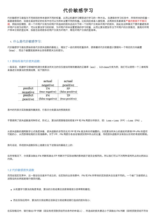
1.1 原始标准代价损失函数:⼀般来说,机器学习领域的检测分类算法所关注的仅仅是如何得到最⾼的正确率(acc),以2-class分类为例,我们可以使⽤⼀个⼆维矩阵来描述分类算法的预测结果,如下图所⽰:表中的列表⽰实际数据所属类别,⾏表⽰分类算法的预测类别不管使⽤了损失函数是何种形式,形式上,算法的预测错误的即是 FP 和 FN 两部分所表⽰,即:Loss = Loss(FP)+ Loss(FN)。
从损失函数的通⽤数学公式⾓度来看,损失函数的求导优化对 FP 和 FN 是没有任何偏置的。
分类算法所关⼼的是如何使得 FP+FN 的值尽可能的⼩,从⽽获得较⾼的分类准确率。
对于 FP、FN 两部分各⾃在错误实例中所占的⽐重,传统损失函数并没有加以任何的考虑和限制。
换句话说,传统损失函数实际上是建⽴在下述假设的基础之上的:在所有情况下,分类算法做出 FN 判断和做出 FP 判断对于实际结果的影响因⼦是完全相同的。
所以我们可以不对两种误判所占的⽐例加以约束。
esscher鞅测度 -回复
esscher鞅测度-回复关于esscher鞅测度的介绍和应用。
鞅理论是概率论和随机过程领域中的一个重要分支,在金融衍生品定价和风险管理等领域有广泛应用。
而esscher鞅测度是鞅理论中的一个特殊类型,本文将从介绍鞅的基本概念开始,逐步讲解esscher鞅测度的定义和性质,并探讨其在金融领域中的应用。
鞅(martingale)是概率论中一组随机变量的序列,满足一个重要的条件——在给定过去的信息下,未来的预期值等于当前值。
鞅的概念首先由法国数学家保罗·莱维(Paul Lévy)在20世纪初提出,并在之后由一系列数学家进一步发展完善。
为了更好地理解鞅的定义和性质,我们以一个股票价格模型为例。
假设现在有一只股票价格为S_t,在t时刻进行观察,我们希望根据已有的信息预测其在未来时刻的价格。
如果该股票价格满足鞅的条件,即E[S_{t+1} S_0,S_1,...,S_t]=S_t,则我们可以说该价格是一个鞅。
这个条件实际上是指在给定过去的所有价格信息后,未来价格的预期值等于当前价格。
在金融领域中,我们经常考虑随机过程的贴现因子。
贴现因子是用于将未来的现金流折算到当前时刻的一个经济量。
常见的贴现因子有风险中性测度,它是在这个测度下股票价格是鞅。
不过,在实际应用中,风险中性测度往往难以计算或者不一定存在,这时esscher鞅测度就成为一个很有用的工具。
esscher鞅测度是一种基于鞅的概率测度,其定义是对鞅的原始测度进行调整,使得股票价格在新测度下依然成为鞅。
具体来说,对于每个时刻t,esscher鞅测度的调整是通过乘以一个补偿项来实现的。
这个补偿项通常取为贴现因子的一个函数,其形式为exp(-λS_t),其中λ是一个正的调整参数。
通过这样的调整,我们在新的测度下得到的股票价格序列依然满足鞅的条件。
esscher鞅测度的应用主要在金融衍生品定价和风险管理中。
在金融衍生品定价中,我们经常需要对未来现金流进行折现,而esscher鞅测度提供了一种对未来现金流进行折现的方法,从而可以确定一个较为合理的价格范围。
自动归因算法

自动归因算法
自动归因算法是一种基于梯度的归因算法,该算法普遍认为神经网络的输出对每个输入单元的梯度可以反映输入单元的重要性。
以下是该算法的一种解释:
自动归因算法会将输入单元的重要性建模为梯度与输入单元值的逐元素乘积。
梯度仅能反映输入单元的局部重要性,而平滑梯度和集成梯度算法将重要性建模为平均梯度与输入单元值的逐元素乘积,其中这两种方法中的平均梯度分别指输入样本邻域内梯度的平均值或输入样本到基准点间线性插值点的梯度平均值。
类似地,Grad-CAM算法采用网络输出对每个channel中所有特征梯度的平均值,来计算重要性分数。
进一步,Expected Gradients算法认为,选择单个基准点往往会导致有偏的归因结果,从而提出将重要性建模为不同基准点下的集成梯度。
以上内容仅供参考,建议查阅关于自动归因算法的资料获取更全面的信息。
- 1、下载文档前请自行甄别文档内容的完整性,平台不提供额外的编辑、内容补充、找答案等附加服务。
- 2、"仅部分预览"的文档,不可在线预览部分如存在完整性等问题,可反馈申请退款(可完整预览的文档不适用该条件!)。
- 3、如文档侵犯您的权益,请联系客服反馈,我们会尽快为您处理(人工客服工作时间:9:00-18:30)。
Kernel Basis PursuitVincent Guigue,Alain Rakotomamonjy,St´e phane Canu1 Lab.Perception,Syst`e mes,Information-CNRS-FRE2645 Avenue de l’Universit´e,76801St´Etienne du Rouvray{Vincent.Guigue,Alain.Rakoto,Stephane.Canu}@insa-rouen.frR´e sum´e:Les m´e thodes`a noyaux sont largement utilis´e es dans le domaine de la r´e gression.Cependant,ce type de probl`e me aboutit`a deux questions r´e currentes: comment optimiser le noyau et comment r´e gler le compromis biais-variance? L’utilisation de noyaux multiples et le calcul du chemin complet de r´e gularisation permettent de faire face simplement et efficacement`a ces deux tˆa ches.L’intro-duction de noyaux multiples est´e galement un moyen de fusionner des sources d’information h´e t´e rog`e nes.Notre approche est inspir´e e de l’algorithme Basis Pursuit(Chen et al.,1998). Nous avons suivi la m´e thode de Vincent et Bengio pour la non-lin´e arisation du Basis Pursuit(Vincent&Bengio,2002).Cet article pr´e sente une solution simple et parcimonieuse pour le probl`e me de r´e gression par m´e thode`a noyaux multiples.Nous avons utilis´e la formulation du LASSO(Least Absolute Shrinkage and Selection Operator)(Tibshirani,1996), bas´e e sur une r´e gularisation L1,et l’algorithme du LARS(Stepwise Least Angle Regression)(Efron et al.,2004)pour la r´e r´e gularisation L1est un gage de parcimonie tandis que le calcul du chemin complet de r´e gularisation, via le LARS,permet de d´efinir de nouveaux crit`e res pour trouver le compro-mis biais-variance optimal.Nous pr´e senterons´e galement une heuristique pour le r´e glage des param`e tres du noyau,afin de rendre la m´e thode compl`e tement non param´e trique.Mots-cl´e s:R´e gression,Noyaux Multiples,LASSO,M´e thode Non-Param´e triqueAbstract:Kernel methods have been widely used in the context of regression. But every problem leads to two major tasks:optimizing the kernel and setting the fitness-regularization ing multiple kernels and Basis Pursuit is a way to face easily and efficiently these two tasks.On top of that,it enables us to deal with multiple and heterogeneous sources of information.Our approach is inspired by the Basis Pursuit algorithm(Chen et al.,1998).We use Vincent and Bengio’s method(Vincent&Bengio,2002)to kernelize the Basis Pursuit and introduce the ability of mixing heterogeneous sources of information.CAp2005This article aims at presenting an easy,efficient and sparse solution to the multipleKernel Basis Pursuit problem.We will use the Least Absolute Shrinkage andSelection Operator(LASSO)formulation(Tibshirani,1996)(L1regularization),and the Stepwise Least Angle Regression(LARS)algorithm(Efron et al.,2004)as solver.The LARS provides a fast and sparse solution to the LASSO.The factthat it computes the optimal regularization path enables us to propose new auto-adaptive hyper-parameters for thefitness-regularization compromise.We willalso propose some heuristics to choose the kernel parameters.Finally,we aim atproposing a parameter free,sparse and fast regression method.Key words:Regression,Multiple Kernels,LASSO,Parameter Free.1IntroductionThe context of our work is the following:we wish to estimate the functional dependency between an input x and an output y of a system given a set of examples{(x i,y i),x i∈X,y i∈Y,i=1...n}which have been drawn i.i.d from an unknown probability law P(X,Y).Thus,our aim is to recover the function f which minimizes the following riskR[f]=E{(f(X)−Y)2}(1) but as P(X,Y)is unknown,we have to look for the function f which minimizes theempirical risk:R emp[f]=ni=1(f(x i)−y i)2(2)This problem is ill-posed and a classical way to turn it into a well-posed one is to use regularization theory(Tikhonov&Ars´e nin,1977;Girosi et al.,1995).In this con-text,the solution of the problem is the function f∈H that minimizes the regularized empirical risk:R reg[f]=1Kernel Basis Pursuit method consisting in adding functions from a dictionary.The bias-variance problem involves several parameters,especially the kernel parameters and the hyper-parameter trading between goodness-of-fit and regularization.Our solution is based onℓ1regularization,we useΩ= β ℓ1in equation3.This for-mulation is called the Least Absolute Shrinkage and Selection Operator(LASSO)(Tib-shirani,1996),it will enable us to improve sparsity.Our solver relies on the Stepwise Least Angle Regression(LARS)algorithm(Efron et al.,2004),which is an iterative forward algorithm.Thus,the sparsity of the solution is closely linked to the efficiency of the method.We use Vincent and Bengio’s strategy(Vincent&Bengio,2002)to kernelize the resulting method.Finally,we end at the Kernel Basis Pursuit algorithm. Associated with this learning problem,there are two major tasks to build a good re-gression function with kernel:optimizing the kernel and choosing a good compromise betweenfitness and regularization.The use of multiple kernels is a way to make the first task easier.We will use the optimal path regularization properties of the LARS to propose new heuristics,in order to set dynamically thefitness-regularization compro-mise.In section2,we will compare two approaches to the question of sparsity:the Match-ing Pursuit and the Basis Pursuit.We will explain the building and the use of the multiple kernels,combined with the LARS in section3.Our results on synthetic and real data are presented in section4.Section5gives our conclusions and perspectives on this work.2Basis vs Matching PursuitTwo common strategies are available to face the problem of building a sparse regres-sion function f.Thefirst one relies on an iterative building of f.At each step k,the comparison between the target y and the function f k leads to add a new source of infor-mation to build f k+1.This approach is fast but it is greedy and thus sub-optimal.The second solution consists in solving a learning problem,by minimizing the regularized empirical risk of equation3.Mallat and Zhang introduced the Matching Pursuit algorithm(Mallat&Zhang,1993): they proposed to construct a regression function f as a linear combination of elemen-tary functions g picked from afinite redundant dictionary D.This algorithm is iterative and one new function g is introduced at each step,associated with a weightβ.At step k,we get the following approximation of f:f k=ki=1βi g i(5)Given R k,the residue generated by f k,the function g k+1and its associated weight βk+1are selected according to:(g k+1,αk+1)=argmin g∈D,β∈R R k−βg 2(6) The improvements described by Pati et al.(Orthogonal Matching Pursuit algorithm) (Pati et al.,1993)keep the same framework,but optimize all the weightsβi at eachCAp2005step.A third algorithm called pre-fitting(Vincent&Bengio,2002)enables us to choose (g k+1,βk+1)according to R k+1.All those methods are iterative and greedy.The different variations improve the weights or the choice of the function g but the main characteristic remains unchanged. Matchin Pursuit does not allow to get rid of a previous source of information,which means that its solution is sub-optimal.The approach of Chen et al.(Chen et al.,1998) is really different:they consider the whole dictionary of functions and look for the best linear solution(equation5)to estimate y,namely,the solution which minimizes theregularized empirical ingΩ= β ℓ1leads to the LASSO formulation.Such aformulation requires costly and complex linear programming(Chen,1995)or modified EM implementation(Grandvalet,1998)to be solved.Finally it enables them tofind an exact solution to the regularized learning problem.The Stepwise Least Angle Regression(LARS)(Efron et al.,2004)offers new oppor-tunities,by combining an iterative and efficient approach with the exact solution of the LASSO.The fact that the LARS begins with an empty set of variables,combined with the sparsity of the solution explains the efficiency of the method.The ability of deleting dynamically useless variables enables the method to converge to the exact solution of the LASSO problem.3Learning with multiple kernels3.1Building a multiple kernel regression functionVincent and Bengio(Vincent&Bengio,2002)propose to treat the kernel K exactly in the same way as the matrix X.Each column of K is then a source of information that can be added to the linear regression model f.Given an input vector x and a parametric mapping functionΦθdefined byΦθ:R d Fx→Φθ(x)=Kθ(x,·)(7)where F is the spanned feature space,we consider Kθ(x,.)as a source of information. It becomes easy to deal with multiple mapping functionsΦi.The multiple resulting kernels K i are placed side by side in a big matrix K:K= K1...K i...K N (8) N is the number of kernels.In this situation,each source of information K i(x j,·)is characterized by a point x j of the learning set and a kernel parameter i.The number of information sources is then s=nN and K∈R n×s.The learning problem becomes a variable selection problem where theβi coefficients can be seen as the weights of the sources of information.We simplify the notations:f=Ni=1n j=1βij K i(x j,·)=s i=1βi K(i,·)=Kβ(9)Kernel Basis PursuitIt is important to note that no assumption is made on the kernel K θwhich can be non-positive.K can associate kernels of the same type (e.g.Gaussian)with different parameter values as well as different types of kernels (e.g.Gaussian and polynomial).The resulting matrix K is neither positive definite or square.3.2LARSThe LARS (Efron et al.,2004)is a stepwise iterative algorithm which provides an exact to minimization of the regularized empirical risk (equation 3)with Ω= β ℓ1.We use the following formulation,which is equivalent to the LASSO:min β y −Kβ 2With respect to: β ℓ1≤t (10)We denote by βi the regression coefficient associated to the i th source of information and by ˆy (j )=Kβ(j )the regression function at step j .More generally,we will use exponent to characterize the RS is made of the following main steps:1.Initialization:the active set of information source A is empty,all βcoefficients are set to zero.putation of the correlation between the sources of information and the residue.The residue R is defined by R =y −ˆy .3.The most correlated source is added to the active set.A ={A arg max i,θ(|K T θ(x i ,·)R |)}(11)4.Definition of the best direction in the active set:−→u A This is the most expensivepart of the algorithm in time computation since it requires the inversion of thematrix K T A K A .5.The original part of the algorithm resides in the computation of the step γ.The idea is to compute γsuch as two functions are equi-correlated with the residue (cf Fig.1)whereas Ordinary Least Square (OLS)algorithm defines γsuch as −→u A and −−−−−→ˆy (j +1),y become orthogonal.6.The regression function is updated:ˆy (j +1)=ˆy (j )+γ−→u A (12)It is necessary to introduce the ability of suppressing a function from the active set to fit the LASSO solution,namely to turn the forward algorithm into a stepwise method.When the sign of a βi changes during the update (equation (12),the step γis reduced so that this βi becomes zero.Then,the corresponding source is removed from the active set and an optimization is performed over the new active set.Solving the LASSO is really fast with this method,due to the fact that it is both forward and sparse.The first steps are not expensive,because of the small size of theCAp2005active set,then it becomes more and more time consuming with iterations.But the sparsity ofℓ1regularization limits the number of required RS begins with an empty active set whereas linear programming and other backward methods begin with all functions and require to solve high dimensional linear system to put irrelevant coefficients to zero.Given the fact that only one point is added(or removed)during an iteration,it is possible to update the inverted matrix of step four instead of fully computing it.This leads to a simple-LARS algorithm,similarly to the simple-SVM formulation(Loosli et al.,2004),which also increases the speed of the method.3.3Optimization of regularization parameterOne of the most interesting property of the LARS is the fact that it computes the whole regularization path.The regularization parameterλof equation3is equivalent to the bound t of equation10.At each step,the introduction of a new source of information leads to an optimal solution,corresponding to a given value of t.In the other classical algorithms,λis set a priori and optimized by cross-validation.The LARS enables us to compute a set of optimal solutions corresponding to different values of t,with only one learning stage.It also enables us to optimize the value of t dynamically,during the learning stage.Finding a good setting for t is very important:when t becomes too large,the re-sulting regression function is the same as the Ordinary Least Square(OLS)regression function.Hence,it requires the resolution of linear system of size s×s.Early stopping should enable us to decrease the time computation(which is linked to the sparsity of the solution)as well as to improve the generalization of the learning(by regularizing).3.3.1Different compromise parametersThe computation of the complete regularization path offers the opportunity to set the compromise parameter dynamically(Bach et al.,2004).Thefirst step is to look for different expressions of the regularization parameter t of equation(10).The aim is to find the most meaningful one,namely the easiest way to set this parameter.Kernel Basis Pursuit -The original formulation of the LARS relies on the compromise parameter t which is a bound on the sum of the absolute values of theβcoefficients.t is difficult to set because it is somewhat meaningless.-It is possible to apply Ljung criterion(Ljung,1987)on the autocorrelation of the residue.The parameter is then a threshold which decides when the residue can be considered as white noise.-Another solution consists in the study of the evolution of loss functionℓ(y i,f jθ(x i))with regards to the step j.The criterion is a bound on the variation of this cost.-ν-LARS.It is possible to define a criterion on the number of support vectors or on the rate of support vectors among the learning set.It is important to note that theνthreshold is then a hard threshold,whereas in theν-SVM method whereνcan be seen as an upper bound on the rate of support vectors(Sch¨o lkopf&Smola, 2002).However,all these methods require the setting of a parameter a priori.The value of this parameter is estimated by cross-validation.3.3.2Trap sourceWe propose another method based on a trap parameter.The idea is to introduce one or many sources of information that we do not want to use.When the most correlated source with the residue belongs to the trap set,the learning procedure is stopped.The trap sources of information can be built on different heuristics:-according to the original signal noise when there exists prior knowledge on the data,-with regards to the distribution of the learning points,to prevent overfitting(cfFig.2),in this case,a Gaussian kernel K=Kσof is added to the informationsources,withσof very small,-by adding random variables among the sources of information(with Gaussian or uniform distribution).This kind of heuristic has already been used in variable selection(Bi et al.,2003).The use of a trap scale is closely linked to the way that LARS selects the sources of information.As seen in section3.2,the selected source of information at a given iteration is the most correlated with the residue.Those heuristics are based on the meaning of the trap scale:the learning stage should be stopped when the residue is most correlated respectively with the noise,with only one source of information or with an independent random variable generated according to the uniform distribution. This means that no more relevant information is present in the sources that are not in the active set.CAp2005Figure2:Illustration of a trap scale based on overfitting heuristic(Gaussian kernel).When Kσ2(x,·)is the most correlated source of information with the residue,it meansthat the error is caused by only one point,it is a way to detect the beginning of overfit-ting.3.4Optimizing kernel parametersInstead of searching an optimal parameter(or parameter vector)for the problem,we propose tofind a key scale tofit the regions where there are the highest point density in the input space.We aim atfinding a reference Gaussian parameter so that the two near-est points in the input space have few influence on each other.This reference parameter represents the smallest bandwidth which can be interesting for a given problem.Then, we propose to build a series of bigger Gaussian parameters from this scale tofit the different densities of points that can append in the whole input space.A one nearest neighbors is performed on the training data.To describe high density regions,we focus on the shortest distances between neighbors.The key distance D k is defined as the distance between x i and x j,the two nearest points in the input space.The corresponding key Gaussian parameterσk is defined so that:K(x i,x j)=12πσk exp −D2kKernel Basis Pursuit4ExperimentsWe illustrate the efficiency of the methodology on synthetic and real data.Tables1and 2present the results with two different algorithms:the SVM and the LARS.We use four strategies to stop the learning stage of the LARS.-LARS- i|βi|is the classical method where a bound is defined on the sum of the regression coefficient.This bound is estimated by cross validation.-ν-LARS is based on the fraction of support vectors.νis also estimated by cross validation.-LARS-RV relies on the introduction of random variables as sources of informa-tion.The learning stage is stopped when one of these sources is picked up as most correlated with the residue.-LARS-σs relies also on a trap scale,but this scale is built according to the dis-tribution the learning set.Selecting a source in this trap scale can be seen as overfitting.We useσs=σk of equation(13).To validate this approach,we compare the results with classical Gaussianǫ-SVM re-gression,Parametersǫ,C andσare optimized by cross validation.In order to distin-guish the benefit of the LARS from the benefits of the multiple kernel learning,we also give the results of LARS algorithm combined with single kernel.4.1Synthetic dataThe learning of cos(exp(ωt))regression function,with random sampling show the mul-tiple kernel interest.We try to identify:f(t)=cos(exp(ωt))+b(t)(15) where b(t)is a Gaussian white noise of varianceσ2b=0.4.t∈[0,2]is drawn ac-cording to a uniform distribution,ω=2.4.We also tested the method over classical synthetic data described by Donoho and Johnstone(Donoho&Johnstone,1994).For those signals,we took t∈[0,1],drawn according to a uniform distribution.We use200points for the learning set and1000points for the testing set.The noise is added only on the learning set.Parameters(ν, i|βi|...)are computed by cross validation on the learning set.Table1presents the results over30runs for each data base.These results point out the sparsity and the efficiency of LARS solutions.Figure3 illustrates how multiple kernel learning enables the regression function tofit the local frequency of the model.It also shows that selected points belong higher and higher scales with iterations.Indeed,the correlation with the residue can be seen as an ener-getic criterion:when the amplitude of the signal remain constant,there is more energy in the low frequency part of the signal.That is why thefirst selected sources of infor-mation describe those parts of the signal.The results with different Donoho’s synthetic signals enable us to distinguish the benefits of the LARS method from the benefits ofCAp 2005Algorithmǫ-SVM ν-LARS cos(exp(t ))0.16±0.016155.40.17±0.01512000.041±0.006837.1000.039±0.005932.800Blocks 1.18±0.2045.3001.19±0.17210.028±0.007025.6340.028±0.006533.933HeaviSine 0.48±0.1251.43110.49±0.12404Algorithm LARS-P i |βi |LARS-RV cos(exp(t ))0.13±0.014122.4170.13±0.016121.470.035±0.00624600.035±0.007549.800Blocks 0.95±0.3434.02130.96±0.2542.3560.032±0.00502700.033±0.005927.330HeaviSine 0.50±0.1451.3000.49±0.1548.224Table 1:Results of SVM and LARS for the cos(exp(t ))and Donoho’s classical func-tions estimation.Mean and standard deviation of MSE on the test set (30runs),number of support vectors used for each solution,number of best performances.Kernel Basis PursuitFigure3:These illustratingfigures explain the learning of the cos(exp(ωt))function with low noise level.Selected learning points belong to different scales,depending on the local frequency of the function to learn.Rightfigure shows that selected points belong higher and higher scales with iterations,namely,the sources of information correlated with the residue are more and more local with iterations.the multiple kernels.The LARS improves the sparsity of the solution,whereas the multiple kernels improve the results on signals that require a multiple scale approach.ǫ-SVM achieves the best results for Ramp and HeaviSine signals.This can be ex-plained by the fact that the Ramp and HeaviSine signals are almost uniform in term of frequency.Theǫtube algorithm of the SVM regression is especially efficient on this kind of problem.It is important to note that LARS-RV and LARS-σs are parameter free methods when combined with the heuristic described in section3.4.Best results are achieved with LARS- i|βi|,however,LARS-RV results are almost equivalent without any parame-ters.4.2Real dataExperiments are carried out over regression data bases pyrim and triazines available in the UCI repository(Blake&Merz,1998).We compare our results with(Chang&Lin, 2005).The experimental procedure for real data is the following one:Thirty training/testing set are produced randomly,table2presents mean and standard deviation of MSE(mean square error)on the test set.80%of the points are used for training and the remaining paramters(ν, i|βi|...)are computed by cross validation on the learning set.The results obtained with LARS algorithm are either equivalent to Chang and Lin’s ones or better.ǫ-SVM solution is not really competitive but it gives an interesting information on the number of support vectors required for each RS-RV and LARS-σs results are very interesting:they are parameter free using the heuristic describe in section3.4,moreover the LARS-RV achieves the best results for pyrim.CAp2005Algo SVMǫ-SVM RV0.009±0.01637.1100.011±0.00931.20triazines0.021±0.005−−0.022±0.00637.00Algo LARSPi|βi|σs0.007±0.00638.08170.020±0.00552.038Table2:Results of SVM and LARS for the different regression database.Mean and standard deviation of MSE on the test set(30runs),number of support vectors used for each solution,number of best performances.5ConclusionThis paper enables us to meet two objectives:proposing a sparse kernel-based solution for the regression problem and introducing new solutions for the bias-variance compro-mise problem.The LARS offers opportunities for both problems.It gives an exact solution to the LASSO problem,which is sparse due toℓ1regularization.The ability of dealing with multiple kernels allows rough setting for the kernel parameters.Then,LARS algo-rithm optimizes the parameters at each iteration,selecting a new point in the optimal scale.The fact that the LARS computes the regularization path offers efficient and non parametric settings for the compromise parameter.This methodology gives good results on synthetic and real data.In the meantime,the required time computation is reduced compared with SVM,due to the sparsity of the obtained solutions.The perspectives of this work are threefold.We have to test LARS-methods on more databases to evaluate all properties.We also want to improve the multiple kernel build-ing.Indeed,the use of the currentσk often leads to a slight overfitting and to less sparse solutions.Finally,we will analyze the LARS-RV results deeper,to explain the good results and possibly improve them.ReferencesB ACH F.,T HIBAUX R.&J ORDAN M.(2004).Computing regularization paths for learningKernel Basis Pursuitmultiple kernels.In Advances in Neural Information Processing Systems,volume17.B I J.,B ENNETT K.,E MBRECHTS M.,B RENEMAN C.&S ONG M.(2003).Dimensionality reduction via sparse support vector machines.Journal of Machine Learning Research,3,1229–1243.B LAKE C.&M ERZ C.(1998).UCI rep.of machine learning databases.C HANG M.&L IN C.(2005).Leave-one-out bounds for support vector regression model se-lection.Neural Computation.C HEN S.(1995).Basis Pursuit.PhD thesis,Department of Statistics,Stanford University.C HEN S.,D ONOHO D.&S AUNDERS M.(1998).Atomic decomposition by basis pursuit. SIAM Journal on Scientific Computing,20(1),33–61.D ONOHO D.&J OHNSTONE I.(1994).Ideal spatial adaptation by wavelet shrinkage. Biometrika,81,425–455.E FRON B.,H ASTIE T.,J OHNSTONE I.&T IBSHIRANI R.(2004).Least angle regression. Annals of statistics,32(2),407–499.G IROSI F.,J ONES M.&P OGGIO T.(1995).Regularization theory and neural networks archi-tectures.Neural Computation,7(2),219–269.G RANDVALET Y.(1998).Least absolute shrinkage is equivalent to quadratic penalization.In ICANN,p.201–206.K IMELDORF G.&W AHBA G.(1971).Some results on Tchebycheffian spline functions.J. Math.Anal.Applic.,33,82–95.L JUNG L.(1987).System Identification-Theory for the User.L OOSLI G.,C ANU S.,V ISHWANATHAN S.,S MOLA A.J.&C HATTOPADHYAY M.(2004). Une boˆıte`a outils rapide et simple pour les svm.In CAp.M ALLAT S.&Z HANG Z.(1993).Matching pursuits with time-frequency dictionaries.IEEE Transactions on Signal Processing,41(12),3397–3415.P ATI Y.C.,R EZAIIFAR R.&K RISHNAPRASAD P.S.(1993).Orthogonal matching pursuits: recursive function approximation with applications to wavelet decomposition.In Proceedings of the27th Asilomar Conference in Signals,Systems,and Computers.S CH¨OLKOPF B.&S MOLA A.(2002).Learning with kernels.T IBSHIRANI R.(1996).Regression shrinkage and selection via the lasso.J.Royal.Statist., 58(1),267–288.T IKHONOV A.&A RS´E NIN V.(1977).Solutions of ill-posed problems.W.H.Winston.V INCENT P.&B ENGIO Y.(2002).Kernel matching pursuit.Machine Learning Journal,48(1), 165–187.W AHBA G.(1990).Spline Models for Observational Data.Series in Applied Mathematics, V ol.59,SIAM.。
