Monte Carlo simulation of nonlinear Couette flow in a dilute gas
Monte Carlo数值模拟法
Monte Carlo 数值模拟法
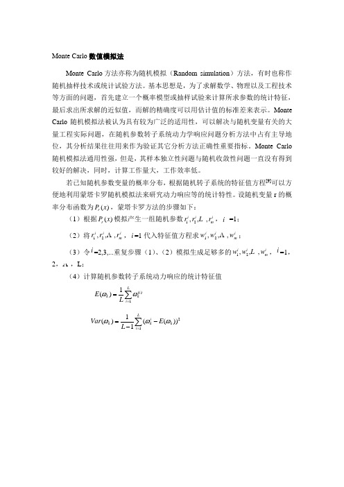
Monte Carlo 方法亦称为随机模拟(Random simulation )方法,有时也称作随机抽样技术或统计试验方法。
基本思想是,为了求解数学、物理以及工程技术等方面的问题,首先建立一个概率模型或抽样试验来计算所求参数的统计特征,最后求出所求解的近似值,而解的精确度可以用估计值的标准差来表示。
Monte Carlo 随机模拟法被认为具有较为广泛的适用性,可以解决与随机变量有关的大量工程实际问题,在随机参数转子系统动力学响应问题分析方法中占有主导地位,其分析结果往往用来作为验证其它分析方法正确性重要指标。
Monte Carlo 随机模拟法通用性强,但是,其样本独立性问题与随机收敛性问题一直没有得到较好的解决,同时,计算工作量大,工作效率低。
若已知随机参数变量的概率分布,根据随机转子系统的特征值方程[9]可以方便地利用蒙塔卡罗随机模拟法来研究动力响应等的统计特性。
设随机变量r 的概率分布函数为()r P x ,蒙塔卡罗方法的步骤如下:
(1)根据()r P x 模拟产生一组随机参数12,,,i i i m r r r ,i =1;
(2)将i m i i r r r ,,,21 ,i =1代入特征值方程求i
m i i w w w ,,,21 ;
(3)令i =2,3,...重复步骤(1)、(2)模拟生成足够多的12,,,i i i m w w w ,i =1,2, ,L ;
(4)计算随机参数转子系统动力响应的统计特征值
()11()L i k k i E L ωω==∑
211()(())1L i k k k i Var E L ωωω==--∑。
衍生品定价的方法

衍生品定价的方法衍生品定价是金融市场中一项重要的活动,通过对金融衍生品进行定价,金融机构可以在市场上买卖这些衍生品来进行风险管理和投资交易。
衍生品定价方法的选择取决于衍生品类型及其特征,下面将介绍一些常见的衍生品定价方法。
1. 基于风险中性定价模型(Risk-neutral Pricing Model)风险中性定价模型是衍生品定价中最常用的方法之一。
该模型的基本思想是假设市场处于风险中性状态,即投资者对风险是中立的。
根据这一假设,可以通过构建动态投资组合,在风险中性世界中对衍生品进行定价。
此方法常用于期权定价,如布莱克-斯科尔斯期权定价模型就是基于风险中性定价原理。
2. 基于随机模型(Stochastic Models)随机模型是另一种常用的衍生品定价方法,该方法将金融市场的价格变动建模为一个随机过程。
常见的随机模型包括布朗运动模型、几何布朗运动模型等。
通过使用随机模型,可以模拟金融资产的价格变动,并根据模型的参数进行衍生品的定价。
3. 基于蒙特卡洛模拟(Monte Carlo Simulation)蒙特卡洛模拟是一种基于随机抽样的方法,通过生成大量的随机路径,来估计衍生品的价值。
该方法适用于复杂的衍生品,因为它可以模拟各种市场条件和价格变动的情况。
蒙特卡洛模拟可以为衍生品的定价提供更准确的估计,但同时需要大量的计算资源和时间。
4. 基于树模型(Tree Models)树模型是一种常用的离散化模型,将时间和价格通过建立树状结构进行离散化。
在树模型中,每个节点表示时间和价格的特定组合。
可以通过构建树模型,从当前价格开始,逐步推导出衍生品的价值。
常见的树模型包括二叉树模型和多项式树模型。
以上介绍的方法只是衍生品定价中的一部分,实际上,衍生品定价方法的选择还取决于市场的特点、金融机构的需求以及投资者的偏好。
因此,在实际应用中,常常需要进行方法的选择和参数的估计等工作,以确保定价结果的准确性和可靠性。
衍生品定价是金融市场中极为重要的一个环节,对于金融机构和投资者来说,了解和掌握衍生品的定价方法是进行投资决策和风险管理的基础。
蒙特卡罗方法 (Monte Carlo simulation)
[0, )
• The random vector is uniformly distributed on the region [0,d)×[0,). Accordingly, it has probability density function 1/d. • The probability that the needle will cross one of the lines is given by the integral
2014-8-27
Monte Carlo模拟
18
4.Monte Carlo算法的主要组成部分
Monte Carlo算法的主要组成部分 概率密度函数(pdf) 必须给出描述一个物理系统的一组概率密度函数;
随机数产生器 能够产生在区间[0,1]上均匀分布的随机数 抽样规则 如何从在区间[0,1]上均匀分布的随机数出发,随机抽 取服从给定的pdf的随机变量;
p
2014-8-27
0
l sin
0
1 d
2l dAd d
Monte Carlo模拟 8
2.Monte Carlo方法简史 Enrico Fermi
• 1930年,利用Monte Carlo方法研究中子的扩散 • 并设计了一个Monte Carlo机械装置,Fermiac,用于计算核 反应堆的临界状态
2014-8-27
Monte Carlo模拟
12
Monte Carlo模拟
第一章 引言 (Introduction)
1. 2. 3. 4. Monte Monte Monte Monte Carlo方法 Carlo方法简史 Carlo模拟的应用 Carlo算法的主要组成部分
蒙特卡洛模拟法

蒙特卡洛模拟法
蒙特卡洛模拟法(Monte Carlo Simulation)是一种概率模型,用于模拟复杂的系统。
它是通过大量随机数据的模拟,来获得对真实情况的大致模拟,从而获得解决复杂问题的决策性结果。
蒙特卡洛模拟法在投资、金融风险分析和管理、保险理论研究、原油价格预测、医学研究、生物化学等领域有着广泛的应用。
它可以用来研究战略游戏、疾病传播模型、统计检验、社会网络分析、概率计算等。
蒙特卡洛模拟的基本思想是:在模型中模拟某种随机事件,通过模拟结果,来推断出最佳解决方案。
蒙特卡洛模拟
蒙特卡洛模拟风险分析是我们制定的每个决策的一部分。
我们一直面对着不确定,不明确和变异。
甚至我们无法获得信息,我们不能准确的预测未来。
蒙特卡洛模拟( Monte Carlo simulation)让您看到了您决策的所有可能的输出,并评估风险,允许在不确定的情况下制定更好的决策。
什么是蒙特卡洛模拟( Monte Carlo simulation)蒙特卡洛模拟( Monte Carlo simulation)是一种计算机数学技术,允许人们在定量分析和决策制定过程中量化风险。
这项技术被专家们用于各种不同的领域,比如财经,项目管理,能源,生产,工程,研究和开发,保险,石油&天然气,物流和环境。
蒙特卡洛模拟( Monte Carlo simulation)提供给了决策制定者大范围的可能输出和任意行动选择将会发生的概率。
它显示了极端的可能性-最的输出,最保守的输出-以及对于中间路线决策的最可能的结果。
这项技术首先被从事原子弹工作的科学家使用;它被命名为蒙特卡洛,摩纳哥有名的娱乐旅游胜地。
它是在二战的时候被传入的,蒙特卡洛模拟( Monte Carlo simulation)现在已经被用于建模各种物理和概念系统。
蒙特卡洛模拟( Monte Carlo simulation)是如何工作的蒙特卡洛模拟( Monte Carlo simulation)通过构建可能结果的模型-通过替换任意存在固有不确定性的因子的一定范围的值(概率分布)-来执行风险分析。
它一次又一次的计算结果,每次使用一个从概率分布获得的不同随机数集。
根据不确定数和为他们制定的范围,蒙特卡洛模拟( Monte Carlo simulation)能够在它完成计算前调用成千上万次的重复计算。
蒙特卡洛模拟( Monte Carlo simulation)产生可能结果输出值的分布。
通过使用概率分布,变量能够拥有不同结果发生的不同概率。
概率分布是一种用来描述风险分析的变量中的不确定性的更加可行的方法。
蒙特卡罗(Monte Carlo)方法简介

蒙特卡罗(Monte Carlo)方法简介蒙特卡罗(Monte Carlo)方法简介蒙特卡罗(Monte Carlo)方法,也称为计算机随机模拟方法,是一种基于"随机数"的计算方法。
一起源这一方法源于美国在第二次世界大战进研制原子弹的"曼哈顿计划"。
Monte Carlo方法创始人主要是这四位:Stanislaw Marcin Ulam, Enrico Fermi, John von Neumann(学计算机的肯定都认识这个牛人吧)和Nicholas Metropolis。
Stanislaw Marcin Ulam是波兰裔美籍数学家,早年是研究拓扑的,后因参与曼哈顿工程,兴趣遂转向应用数学,他首先提出用Monte Carlo方法解决计算数学中的一些问题,然后又将其应用到解决链式反应的理论中去,可以说是MC方法的奠基人;Enrico Fermi是个物理大牛,理论和实验同时都是大牛,这在物理界很少见,在“物理大牛的八卦”那篇文章里提到这个人很多次,对于这么牛的人只能是英年早逝了(别说我嘴损啊,上帝都嫉妒!);John von Neumann可以说是计算机界的牛顿吧,太牛了,结果和Fermi一样,被上帝嫉妒了;Nicholas Metropolis,希腊裔美籍数学家,物理学家,计算机科学家,这个人对Monte Carlo方法做的贡献相当大,正式由于他提出的一种什么算法(名字忘了),才使得Monte Carlo方法能够得到如此广泛的应用,这人现在还活着,与前几位牛人不同,Metropolis很专一,他一生主要的贡献就是Monte Carlo方法。
蒙特卡罗方法的名字来源于摩纳哥的一个城市蒙地卡罗,该城市以赌博业闻名,而蒙特•罗方法正是以概率为基础的方法。
与它对应的是确定性算法。
二解决问题的基本思路Monte Carlo方法的基本思想很早以前就被人们所发现和利用。
早在17世纪,人们就知道用事件发生的"频率"来决定事件的"概率"。
数学建模十大经典算法
数学建模十大经典算法数学建模是将现实问题转化为数学模型,并利用数学方法进行求解的过程。
下面是数学建模中常用的十大经典算法:1.线性规划(Linear Programming):通过确定一组线性约束条件,求解线性目标函数的最优解。
2.整数规划(Integer Programming):在线性规划的基础上,要求变量取整数值,求解整数目标函数的最优解。
3.非线性规划(Nonlinear Programming):目标函数或约束条件存在非线性关系,通过迭代方法求解最优解。
4.动态规划(Dynamic Programming):通过分阶段决策,将复杂问题分解为多个阶段,并存储中间结果,以求解最优解。
5.蒙特卡洛模拟(Monte Carlo Simulation):通过随机抽样和统计分析的方法,模拟系统的行为,得出概率分布或数值近似解。
6.遗传算法(Genetic Algorithm):模拟生物进化过程,通过选择、交叉和变异等操作,寻找最优解。
7.粒子群算法(Particle Swarm Optimization):模拟鸟群或鱼群的行为,通过个体间的信息交流和集体协作,寻找最优解。
8.模拟退火算法(Simulated Annealing):模拟金属退火的过程,通过控制温度和能量变化,寻找最优解。
9.人工神经网络(Artificial Neural Network):模拟生物神经网络的结构和功能,通过训练网络参数,实现问题的分类和预测。
10.遗传规划(Genetic Programming):通过定义适应性函数和基因编码,通过进化算子进行选择、交叉和变异等操作,求解最优模型或算法。
这些算法在不同的数学建模问题中具有广泛的应用,能够帮助解决复杂的实际问题。
什麼是蒙地卡罗方法
什麼是「蒙地卡羅方法」?它是一種數值方法,利用亂數取樣(random sampling) 模擬來解決數學問題。
一般公認蒙地卡羅方法一詞為著名數學家John von Neumann 等人於1949年一篇名為「The Monte Carlo method」所提出。
其實,此方法的理論基礎於更早時候已為人所知,只不過用手動產生亂數來解決問題,是一件費時又費力的繁瑣工作,必須等到電腦時代,使此繁複計算工作才變得實際可執行為什麼取名「蒙地卡羅方法」?在數學上,所謂產生亂數,就是從一給定的數集合中選出的數,若從集合中不按順序隨機選取其中數字,這就叫是亂數,若是被選到的機率相同,這就叫是一均勻亂數。
例如擲骰子,1點至6點骰子出現機率均等。
雖然,現在科學研究中經常是利用電腦產生均勻分佈於[0, 1] 之間的數,但早期最簡單方式是由賭場輪盤以機械方式產生亂數。
這也是為何以摩洛歌首都--蒙地卡羅(賭城)為名的緣故[例題:求圓周率π ]利用電腦產生均勻分佈於[0, 1] 之間的數為點X、Y座標位置,由於點座標均勻分佈在0 ~ 1之間,所以落在某區域之點數目與其面積成正比,只要將落在圓內點數目除以點模擬總數目,即可得圓周率π之數值。
[蒙地卡羅方法基本原理]蒙地卡羅方法到底適合解決哪些問題?舉凡所有具有隨機效應的過程,均可能以蒙地卡羅方法大量模擬單一事件,藉統計上平均值獲得某設定條件下實際最可能測量值。
現今此方法已被應用在許多領域中。
蒙地卡羅方法的基本原理是將所有可能結果發生的機率,定義出一機率密度函數。
將此機率密度函數累加成累積機率函數,調整其值最大值為1,此稱為歸一化(Normalization)。
這也將正確反應出所有事件出現的總機率為1的機率特性,這也為亂數取樣與實際問題模擬建立起連結。
也就是說我們將電腦所產生均勻分佈於[0, 1] 之間的亂數,透過所欲模擬的過程所具有機率分佈函數,模擬出實際問題最可能結果。
Monte Carlo Simulation BasicsA Monte Carlo method is a technique that involves using random numbers and probability to solve problems. The term was coined by S. Ulam and Nicholas Metropolis in reference to games of chance, a popular attraction in Monte Carlo, Monaco (Hoffman, 1998; Metropolis and Ulam, 1949).Computer simulation has to do with using computer models to imitate real life or make predictions. When you create a model, you have a certain number of input parameters and a few equations that use those inputs to give you a set of outputs (or response variables). This type of model is usually deterministic, meaning that you get the same results no matter how many times you re-calculate.Figure 1: A parametric deterministic model maps a set of input variables to a set of output variables.Monte Carlo simulation is a method for iteratively evaluating a deterministic model using sets of random numbers as inputs. This method is often used when the model is complex, nonlinear, or involves more than just a couple uncertain parameters. A simulation can typically involve over 10,000 evaluations of the model, a task which in the past was only practical using super computers.[ ]Deterministic Model ExampleAn example of a deterministic model is a calculation to determine the return on a 5-year investment with an annual interest rate of 7%, compounded monthly. The model is just the equation below:The inputs are the initial investment (P = $1000), annual interest rate (r = 7% = , the compounding period (m = 12 months), and the number of years (Y = 5).Compound Interest ModelPresent value, P1000.00Annual rate, r0.07Periods/Year, m12Years, Y5Future value, F$ 1417.63One of the purposes of a model such as this is to make predictions and try "What If?" scenarios. You can change the inputs and recalculate the model and you'll get a new answer. You might even want to plot a graph of the future value (F) vs. years (Y). In some cases, you may have a fixed interest rate, but what do you do if the interest rate is allowed to change? For this simple equation, you might only care to know a worst/best case scenario, where you calculate the future value based upon the lowest and highest interest rates that you might expect.By using random inputs, you are essentially turning the deterministic model into a stochastic model. Example below demonstrates this concept with a very simple problem.Stochastic Model ExampleA stochastic model is one that involves probability or randomness. In this example, we have an assembly of 4 parts that make up a hinge, with a pin or bolt through the centers of the parts. Looking at the figure below, if A +B +C is greater than D, we're going to have a hard time putting this thing together.Figure : A hinge.Let's say we have a million of each of the different parts, and we randomly select the parts we need in order to assemble the hinge. No two parts are going to be exactly the same size! But, if we have an idea of the range of sizes for each part, then we can simulate the selection and assembly of the parts mathematically.The table below demonstrates this. Each time you press "Calculate", you are simulating the creation of an assembly from a random set of parts. If you ever get a negative clearance, then that means the combination of the parts you have selected will be too large to fit within dimension D. Do you ever get a negativeclearance?This example demonstrates almost all of the steps in a Monte Carlo simulation. The deterministic model is simply D-(A+B+C). We are using uniform distributions to generate the values for each input. All we need to do now is press the "calculate" button a few thousand times, record all the results, create a histogram to visualize the data, and calculate the probability that the parts cannot be assembled.Of course, you don't want to do this manually. That is why there is so much software for automating Monte Carlo simulation.In Example above, we used simple uniform random numbers as the inputs to the model. However, a uniform distribution is not the only way to represent uncertainty. Before describing the steps of the general MC simulation in detail, a little word about uncertainty propagation:The Monte Carlo method is just one of many methods for analyzing uncertainty propagation, where the goal is to determine how random variation, lack of knowledge, or error affects the sensitivity, performance, or reliability of the system that is being modeled. Monte Carlo simulation is categorized as a sampling method because the inputs are randomly generated from probability distributions to simulate the process of sampling from an actual population. So, we try to choose a distribution for the inputs that most closely matches data we already have, or best represents our current state of knowledge. The data generated from the simulation can be represented as probability distributions (or histograms) or converted to error bars, reliability predictions, tolerance zones, and confidence intervals. (See Figure below).Uncertainty PropagationFigure : Schematic showing the principal of stochastic uncertainty propagation. (The basic principle behindMonte Carlo simulation.)If you have made it this far, congratulations! Now for the fun part! The steps in Monte Carlo simulation corresponding to the uncertainty propagation shown in Figure above are fairly simple, and can be easily implemented in software for simple models. All we need to do is follow the five simple steps listed below:Step 1:Create a parametric model, y = f(x1, x2, ..., x q).Step 2:Generate a set of random inputs, x i1, x i2, ..., x iq.Step 3:Evaluate the model and store the results as y i.Step 4:Repeat steps 2 and 3 for i = 1 to n.Step 5:Analyze the results using histograms, summary statistics, confidence intervals, etc.On to an example problemSales Forecasting ExampleOur example of Monte Carlo simulation will be a simplified sales forecast model. Each step of the analysis will be described in detail.The Scenario: Company XYZ wants to know how profitable it will be to market their new gadget, realizing there are many uncertainties associated with market size, expenses, and revenue.The Method: Use a Monte Carlo Simulation to estimate profit and evaluate risk. Step 1: Creating the ModelWe are going to use a top-down approach to create the sales forecast model, starting with:Profit = Income - ExpensesBoth income and expenses are uncertain parameters, but we aren't going to stop here, because one of the purposes of developing a model is to try to break the problem down into more fundamental quantities. Ideally, we want all the inputs to be independent. Does income depend on expenses? If so, our model needs to take this into account somehow.We'll say that Income comes solely from the number of sales (S) multiplied by the profit per sale (P) resulting from an individual purchase of a gadget, so Income = S*P. The profit per sale takes into account the sale price, the initial cost tomanufacturer or purchase the product wholesale, and other transaction fees (credit cards, shipping, etc.). For our purposes, we'll say the P may fluctuate between $47 and $53.We could just leave the number of sales as one of the primary variables, but for this example, Company XYZ generates sales through purchasing leads. The number of sales per month is the number of leads per month (L) multiplied by the conversion rate (R) (the percentage of leads that result in sales). So our final equation for Income is:Income = L*R*PWe'll consider the Expenses to be a combination of fixed overhead (H) plus the total cost of the leads. For this model, the cost of a single lead (C) varies between $ and $. Based upon some market research, Company XYZ expects the number of leads per month (L) to vary between 1200 and 1800. Our final model for Company XYZ's sales forecast is:Profit = L*R*P - (H + L*C)Y = ProfitsX1 = LX2 = CX3 = RX4 = PNotice that H is also part of the equation, but we are going to treat it as a constant in this example. The inputs to the Monte Carlo simulation are just the uncertain parameters (X i).This is not a comprehensive treatment of modeling methods, but I used this example to demonstrate an important concept in uncertainty propagation, namely correlation. After breaking Income and Expenses down into more fundamental and measurable quantities, we found that the number of leads (L) affected both income and expenses. Therefore, income and expenses are not independent. We could probably break the problem down even further, but we won't in this example. We'll assume that L, R, P, H, and C are all independent.Note: In my opinion, it is easier to decompose a model into independent variables (when possible) than to try to mess with correlation between random inputs.Generating Random Numbers using softwareSales Forecast Example - Part IIStep 2: Generating Random InputsThe key to Monte Carlo simulation is generating the set of random inputs. As with any modeling and prediction method, the "garbage in equals garbage out" principle applys. For now, I am going to avoid the questions "How do I know what distribution to use for my inputs?" and "How do I make sure I am using a good random number generator?" and get right to the details of how to implement the method in software.For this example, we're going to use a Uniform Distribution to represent the four uncertain parameters. The inputs are summarized in the table shown below.The table above uses "Min" and "Max" to indicate the uncertainty in L, C, R, and P. To generate a random number between "Min" and "Max", we use the following formula in software(Replacing "min" and "max" with cell references):= min + RAND()*(max-min)You can also use the Random Number Generation tool to kick out a bunch of static random numbers for a few distributions. However, in this example we aregoing to make use of RAND() formula so that every time the worksheet recalculates, a new random number is generated.Let's say we want to run n=5000 evaluations of our model. This is a fairly low number when it comes to Monte Carlo simulation, and you will see why once we begin to analyze the results.Figure :the example sales forecast spreadsheet.To generate 5000 random numbers for L, you simply copy the formula down 5000 rows. You repeat the process for the other variables (except for H, which is constant).Step 3: Evaluating the ModelSince our model is very simple, all we need to do to evaluate the model for each run of the simulation is put the equation in another column next to the inputs, as shown in Figure (the Profit column).Step 4: Run the SimulationWe don't need to write a fancy macro for this example in order to iteratively evaluate our model. We simply copy the formula for profit down 5000 rows, making sure that we use relative references in the formulaRerun the Simulation:Although we still need to analyze the data, we have essentially completed a Monte Carlo simulation. Because we have used the volatile RAND() formula, to re-run the simulation all we have to do is recalculate the worksheet.This may seem like a strange way to implement Monte Carlo simulation, but think about what is going on behind the scenes every time the Worksheet recalculates: (1) 5000 sets of random inputs are generated (2) The model is evaluated for all 5000 sets. Software is handling all of the iteration.A Few Other DistributionsTo generate a random number from a Normal (Gaussian) distribution=NORMINV(rand(),mean,standard_dev)To generate a random number from a Lognormal distribution with median = exp(meanlog), and shape = sdlog, you would use the following formula=LOGINV(RAND(),meanlog,sdlog)To generate a random number from a (2-parameter) Weibull distribution with scale = c, and shape = m, you would use the following formula in Excel:=c*(-LN(1-RAND()))^(1/m)MORE Distribution Functions: checkCreating a HistogramSales Forecast Example - Part IIIIn of this Monte Carlo Simulation example, we completed the actual simulation. We ended up with a column of 5000 possible values (observations) for our single response variable, profit. The last step is to analyze the results. We will start off by creating a histogram, a graphical method for visualizing the results.Figure 1: A Histogram created using a Bar Chart.(From a Monte Carlo simulation using n = 5000 points and 40 bins).We can glean a lot of information from this histogram:•It looks like profit will be positive, most of the time.•The uncertainty is quite large, varying between -1000 to 3400.•The distribution does not look like a perfect Normal distribution.•There doesn't appear to be outliers, truncation, multiple modes, etc.The histogram tells a good story, but in many cases, we want to estimate the probability of being below or above some value, or between a set of specification limits.Figure 4: Example Histogram Created Using a Scatter Plot and Error Bars.Summary StatisticsSales Forecast Example - Part IV of VIn of this Monte Carlo Simulation example, we plotted the results as a in order to visualize the uncertainty in profit. In order to provide a concise summary of the results, it is customary to report the mean, median, standard deviation, standard error, and a few other summary statistics to describe the resulting distribution.Statistics FormulasSample Size (n):::( )Maximum:Mininum:Sample Size (n)The sample size, n, is the number of observations or data points from a single MC simulation. For this example, we obtained n = 5000 simulated observations. Because the Monte Carlo method is stochastic, if we repeat the simulation, we will end up calculating a different set of summary statistics. The larger the sample size, the smaller the difference will be between the repeated simulations.Central Tendancy: Mean and MedianThe sample mean and median statistics describe the central tendancy or "location" of the distribution. The arithmetic mean is simply the average value of the observations.If you sort the results from lowest to highest, the median is the "middle" value or the 50th Percentile, meaning that 50% of the results from the simulation are less than the median. If there is an even number of data points, then the median is the average of the middle two points.Extreme values can have a large impact on the mean, but the median only depends upon the middle point(s). This property makes the median useful for describing the center of skewed distributions such as the Lognormal distribution. If the distribution is symmetric (like the Normal distribution), then the mean and median will be identical.Confidence Intervals for the True PopulationMeanThe sample mean is just an estimate of the true population mean. How accurate is the estimate? You can see by repeating the simulation that the mean is not the same for each simulation.Standard ErrorIf you repeated the Monte Carlo simulation and recorded the sample mean each time, the distribution of the sample mean would end up following a Normal distribution (based upon the Central Limit Theorem). The standard error is a good estimate of the standard deviation of this distribution, assuming that the sample is sufficiently large (n >= 30).The standard error is calculated using the following formula:95% Confidence IntervalThe standard error can be used to calculate confidence intervals for the true population mean. For a 95% 2-sided confidence interval, the Upper Confidence Limit (UCL) and Lower Confidence Limit (LCL) are calculated as:To get a 90% or 99% confidence interval, you would change the value to or , respectively. The value represents the percentile of the standard normal distribution. (You may often see this number rounded to 2).Percentiles and Cumulative ProbabilitiesSales Forecast Example - Part V of VAs a final step in the sales forecast example, we are going to look at how to use the percentile function and percent rank function to estimate important summary statistics from our Monte Carlo simulation results. But first, it will be helpful to talk a bit about the cumulative probability distribution.Creating a Cumulative DistributionIn of this Monte Carlo Simulation example, we plotted the results as a in order to visualize the uncertainty in profit. We are going to augment the histogram by including a graph of the estimated cumulative distribution function (CDF) as shown below.Figure 1: Graph of the estimated cumulative distribution.The reason for showing the CDF along with the histogram is to demonstrate that an estimate of the cumulative probability is simply the percentage of the data points to the left of the point of interest.For example, we might want to know what percentage of the results was less than -$ (the vertical red line on the left). From the graph, the corresponding cumulative probability is about or 5%. Similarly, we can draw a line at $2300 and find that about 95% of the results are less than $2300.It is fairly simple to create the cumulative distribution. Figure 2 shows how you can estimate the CDF by calculating the probabilities using a cumulative sum of the count from the frequency function. You simply divide the cumulative sum by the total number of points.。
用水晶球软件模拟蒙特卡罗

Introduction
Welcome to Crystal Ball 2000, Professional Edition. Crystal Ball 2000, Professional Edition is a sophisticated suite of forecasting, risk analysis, and optimization tools for spreadsheet users. With this suite of tools, you'll be able to answer important decision-making questions such as "What are the risks of this project?" or, "How do we increase profitability?" You'll no longer have to make decisions like these in the dark.
better communication of risk
To run a simulation using Crystal Ball :
1. Setup Spreadsheet :Build a spreadsheet that will calculate the performance measure (e.g., profit) in terms of the inputs (random or not). For random inputs, just enter any number.
风险评估技术-蒙特卡罗模拟分析(Monte Carlo simulation)

蒙特卡罗模拟分析(Monte Carlo simulation)1 概述很多系统过于复杂,无法运用分析技术对不确定性因素的影响进行模拟,但可以通过考虑投入随机变量和运行N次计算(即所谓模拟)的样本,以便获得希望结果的N个可能成果。
描述输入数据的不确定性并开展多项模拟(其中,对输入数据进行抽样以代表可能出现的结果)加以评估。
这种方法可以解决那些借助于分析方法很难理解和解决的复杂状况。
可以使用电子表格和其他常规工具进行系统开发,也可以使用更复杂的工具来满足一些更复杂的要求,很多要求所需的投资较少。
当该技术首次开发时,蒙特卡罗模拟所需的迭代过程缓慢,耗费时间。
但是,随着计算机技术的进步和理论的发展,例如latin-hypercube抽样法使很多应用程序的处理时间几乎变得微不足道。
2 用途蒙特卡罗模拟是评估不确定性因素在各种情况下对系统产生影响的方法。
这种方法通常用来评估各种可能结果的分布及值的频率,例如成本、周期、吞吐量、需求及类似的定量指标。
蒙特卡罗模拟法可以用于两种不同用途:●传统解析模型的不确定性的分布;●解析技术不能解决问题时进行概率计算。
3 输入输入到蒙特卡罗模拟法的是一个系统模型和关于输入类型的信息、不确定性源和期望的输出。
具有不确定性的输入数据被表示为具有一定分布的随机变量,根据不确定性的水平其分布具有或多或少的离散性。
为此,均匀分布、三角分布、正态分布和对数正态分布经常被使用。
4 过程过程如下:●确定尽可能准确代表所研究系统特性的模型或算法;●用随机数将模型运行多次,产生模型(系统模拟)输出。
在模拟不确定性效应的应用场合,模型以方程式的形式提供输入参数与输出之间的关系。
所选择的输入值取自这些参数中代表不确定性特点的适当的概率分布。
●在每一种情况下,计算机以不同的输入运行模型多次(经常到一万次)并产生多种输出。
这些输出可以用传统的统计方法进行处理,以提供均值、方差和置信区间等信息。
下面给出一个模拟例子。
蒙特卡罗仿真方法

主讲人:华北电力大学电子系 张京席
蒙特卡洛(Monte Carlo)简介
蒙特卡洛是摩纳哥公国的一个城镇,拥有 世界闻名的大赌场。
摩纳哥,位于欧洲西南部,地中海边峭壁 上的公国,它建在阿尔卑斯山山脉突出地 中海的悬崖之上,北、东、西三面都与法 国接壤。它的面积只有1.95平方公里,是 世界上海岸线最短的国家,堪称世界“袖 珍国”。摩纳哥依山傍海,景色宜人,犹 如一个五彩缤纷的海滨公园。摩纳哥也因 蒙特卡洛而得名赌博之国。
⎤ ⎥⎦
=
E
⎡ ⎢⎣
1 N2
N n=1
N m=1
X
n
X
m
⎤ ⎥⎦
=
1 N2
NN
E
n=1 m=1
XnXm
∑ ∑ [ ] [ ] ∑ = 1
N
N
E
N2 n=1 m≠n
Xn
E
Xm
+
1 N2
N
E ⎡⎣ X n2 ⎤⎦
n=1
m=1
=
1 N2
⎡⎣(N 2
−
N )Pe2
+
NPe ⎤⎦
方差为:
( ) D ⎡⎣Pˆe(N )⎤⎦ = σ 2
⎫⎪ ⎬ ⎪⎭
=1−
⎛ 2Q ⎜⎜⎝
( ) = 1− 2Q β NPe
β Pe
Pe / N
⎞ ⎟⎟⎠
其中, ∫ Q(x) =
1
∞ −t2
e 2 dt
2π x
1-α是置信水平,若令 { } Pr Pe(1− β ) < Pˆe(N ) < Pe(1+ β ) = 1− α
美赛b题常用模型及算法

美赛b题常用模型及算法美赛(美国大学生数学建模竞赛)B题通常涉及的模型和算法包括但不限于以下几种:1. 线性规划(Linear Programming, LP),在美赛B题中,线性规划经常被用于优化问题的建模和求解。
通过构建线性目标函数和线性约束条件,可以对资源分配、生产计划等问题进行优化。
2. 整数规划(Integer Programming, IP),整数规划是线性规划的扩展,它要求决策变量取整数值。
在美赛B题中,很多实际问题需要考虑决策变量的离散性,因此整数规划经常被用于解决这类问题。
3. 非线性规划(Nonlinear Programming, NLP),有些问题涉及到非线性目标函数或者约束条件,这时候就需要使用非线性规划方法进行建模和求解。
4. 图论算法,美赛B题中经常涉及到网络、路径规划等问题,因此图论算法如最短路径算法(Dijkstra算法、Floyd-Warshall算法)、最小生成树算法(Prim算法、Kruskal算法)等在解决这类问题时非常常用。
5. 动态规划(Dynamic Programming),对于一些具有重叠子问题和最优子结构特点的问题,动态规划是一种非常有效的建模和求解方法。
在美赛B题中,动态规划常常用于求解最优决策序列、资源分配等问题。
6. 蒙特卡洛模拟(Monte Carlo Simulation),对于涉及概率、风险等随机因素的问题,蒙特卡洛模拟可以用来进行概率分布的模拟和随机事件的仿真,是一种常见的建模方法。
7. 数学建模工具的应用,美赛B题中也会涉及到一些特定的数学建模工具,比如微分方程、积分方程、离散事件模拟等,针对具体问题会有相应的数学建模工具被应用。
以上列举的模型和算法只是美赛B题常用的一部分,实际上,根据具体的问题情况,还会涉及到更多不同的数学建模方法和算法。
在解决美赛B题时,需要根据具体问题的特点和要求,选择合适的模型和算法进行建模和求解。
非线性混合效应模型的蒙特卡洛模拟步骤

构建非线性混合模型后,需要采用合适的参数估计方法进行估计。传统的参数估计方法包括极大似然估计法、贝叶斯估计 法等,它们常常基于假设检验噪声分布等前提,在一定条件下可以实现较为准确的估计。而随着技术的发展,深度学习等机器 学习方法也逐渐被应用到非线性混合模型中。与传统参数估计方法相比,深度学习方法对于数据的自适应表征具有更高的鲁棒 性,同时不需要对先验信息进行约束。但其需要较大规模的数据集,并且对参数初始化等因素较为敏感。因此,需要根据实际 情况来选择合适的参数估计方法。
设计模拟数据
进行蒙特卡洛模拟
Perform Monte Carlo simulation.
1. 设定模拟参数:模拟参数包括模型的参数值、观测数据的数量和模拟次 数等因素。在设定参数时应该考虑到实际情况,尽可能逼近真实数据。例如 ,模型的参数值可以通过现有数据的估计值来确定,观测数据的数量应符合 实验要求,而模拟次数应该足够多才能保证结果的可靠性。 2. 进行模拟分析:在设置好参数后,可以使用蒙特卡洛方法对非线性混合 效应模型进行模拟分析。此时需要编写相应的程序,计算观测数据的估计值 和方差,并对结果进行分析和评估。在分析过程中,需要注意结果的稳定性 和可靠性,尤其是在数据量和模拟次数比较小的情况下。同时,还需要对结 果进行可视化处理,以便更好地了解和解释结果。
3. 模型的应用领域和局限性:非线性混合效应模型广泛应用于医学、社会经济、环境科学等领域中。例如,在药物疗效评价中,可以 利用非线性混合效应模型来建立药效-时间关系模型,以更准确地预测药物的治疗效果。然而,非线性混合效应模型也存在一定的局 限性,例如模型参数的解释性不强、模型拟合过程中存在过拟合问题等。对于这些问题,需要对模型假设和数据分析方法进行更深入 的探讨和改进,以提高模型的精度和推广性。
蒙特卡罗方法 (Monte Carlo simulation)
例:a=5,c=1,m=16,I0=1 Î周期=m=16 1,6,15,12,13,2,11,8,9,14,7,4,5,10,3,0,1,6,15, 12,13,2,..
蒙特卡罗方法 (Monte Carlo simulation)
RANDU随机数产生器:
1961年由IBM提出 I n +1 = (65539 × I n ) mod 2 存在严重的问题:Marsaglia效用,存在于所有乘同余方法的产生器
蒙特卡罗方法 (Monte Carlo simulation)
==〉伪随机数(Pseudo-Random Number) Î优点: – – – 占用计算机的内存少; 产生速度快; 可以重复前次的模拟结果,便于程序的找错;
蒙特卡罗方法 (Monte Carlo simulation)
2.3 线性乘同余方法(Linear Congruential Method)
蒙特卡罗方法 (Monte Carlo simulation)
– 所模拟的物理过程要求随机数应具有下列特性:
• 随机数序列应是独立的、互不相关的(uncorrelated):即序列中的任一 子序列应与其它的子序列无关; • 长的周期(long period):实际应用中,随机数都是用数学方法计算出来 的,这些算法具有周期性,即当序列达到一定长度后会重复; • 均匀分布的随机数应满足均匀性(Uniformity):随机数序列应是均匀的、 无偏的,即:如果两个子区间的“面积”相等,则落于这两个子区间内 的随机数的个数影相等。
蒙特卡罗方法 (Monte Carlo simulation)
2.2 随机数的产生 • [0,1]区间上均匀分布的随机数是Monte Carlo模拟的基础,服从 任意分布的随机数序列可以用[0,1]区间均匀分布的随机数序列 作适当的变换火舍选后求得; • [0,1]均匀分布的随机数的产生方法:
运用蒙特卡罗模拟进行风险分析

运用蒙特卡罗模拟进行风险分析蒙特卡罗模拟由著名的摩纳哥赌城而得名,他是一种非常强有力的方法学。
对专业人员来说,这种模拟为方便的解决困难而复杂的实际问题开启了一扇大门。
估计蒙特卡罗模拟最著名的早期使用是诺贝尔奖物理学家Enrico Fermi(有时也说是原子弹之父)在1930年的应用,那时他用一种随机方法来计算刚发现的中子的性质。
蒙特卡罗模拟是曼哈顿计划所用到的模拟的核心部分,在20世纪50年代蒙特卡罗模拟就用在Los Alamos国家实验室发展氢弹的早期工作中,并流行于物理学和运筹学研究领域。
兰德公司和美国空军是这个时期主要的两个负责资助和传播蒙特卡罗方法的组织,今天蒙特卡罗模拟也被广泛应用于不同的领域,包括工程,物理学,研发,商业和金融。
简而言之,蒙特卡罗模拟创造了一种假设的未来,它是通过产生数以千计甚至成千上万的样本结果并分析他们的共性实现的。
在实践中,蒙特卡罗模拟法用于风险分析,风险鉴定,敏感度分析和预测。
模拟的一个替代方法是极其复杂的随机闭合数学模型。
对一个公司的分析,使用研究生层次的高等数学和统计学显然不合逻辑和实际。
一个出色的分析家会使用所有他或她可得的工具以最简单和最实际的方式去得到相同的结果。
任何情况下,建模正确时,蒙特卡罗模拟可以提供与更完美的数学方法相似的答案。
此外,有许多实际生活应用中不存在闭合模型并且唯一的途径就是应用模拟法。
那么,到底什么是蒙特卡罗模拟以及它是怎么工作的?什么是蒙特卡罗模拟?今天,高速计算机使许多过去看来棘手的复杂计算成为可能。
对科学家,工程师,统计学家,管理者,商业分析家和其他人来说,计算机使创建一个模拟现实的模型成为可能,这有助于做出预测,其中一种方法应用于模拟真实系统,它通过调查数以百计甚至数以千计的可能情况来解释随机性和未来不确定性。
结果通过编译后用于决策。
这就是蒙特卡罗模拟的全部内容。
形式最简单的蒙特卡罗模拟是一个随机数字生成器,它对预测,估计和风险分析都很有用。
汽车制造蒙特卡洛模拟及其在公差设计中的应用

成环数 n 不能太大,一般应小于 10 的场合.蒙特卡 洛模拟法可以进行各种随机变量(包括线性、非线性 尺 寸 链 ) 的 模 拟 计 算 ,是 一 种 通 用 的 公 差 分 析 技 术.由于它的计算精度与样本量的平方根成正比,故 需要的样本量很大,模拟次数一般在数万次到几十万 次才能保证计算精度.过去认为蒙特卡洛模拟法计 算时间长,限制了它的使用.随着计算机技术的发 展,计算时间已经不是制约的因素.
公差分析的方法有极值法和统计公差方法两 类.极值法是建立在零件 100%互换的基础上,是一种 最简单的方法,但按极值法计算的公差过于保守,对 加工精度要求提高,增加制造成本.根据概率论与数 理统计理论进行公差分析的方法称为统计公差方法, 统计公差的方法有概率法、修正的概率法、卷积法、 Taguchi 实验法和蒙特卡洛(Monte Carlo)模拟法 等[1,2].概率法是建立在假定封闭环为正态分布、置信 水平为 P=99.73%基础上的;如果改变置信水平,则难 以 进 行 计 算 ,这 与 生 产 的 实 际 要 求 有 时 是 不 相 符 的.卷积法主要应用于线形尺寸链的求解,对非线性 尺寸链要进行线形化处理,会产生舍入误差,影响计 算精度.Taguchi 实验法虽然比较简单,但它要求组
多的 y 值后,再求出 y 的各阶中心矩.最后,根据封
闭环尺寸的分布就可以求解相应的公差.
基于蒙特卡洛模拟的公差分析流程如图 3 所
示.用蒙特卡洛模拟进行公差分析包括以下内容:
(1)概率密度函数.公差设计函数的性质与尺
寸链各组成环尺寸的概率密度函数有关.设 n 为设
计变量的个数,x1, x2 , , xn 是相互独立的尺寸设计变 量(组成环尺寸),则公差设计函数为
(College of Mechanical Engineering,Tianjin University of Science & Technology,Tianjin 300222,China)
- 1、下载文档前请自行甄别文档内容的完整性,平台不提供额外的编辑、内容补充、找答案等附加服务。
- 2、"仅部分预览"的文档,不可在线预览部分如存在完整性等问题,可反馈申请退款(可完整预览的文档不适用该条件!)。
- 3、如文档侵犯您的权益,请联系客服反馈,我们会尽快为您处理(人工客服工作时间:9:00-18:30)。
a r X i v :c o n d -m a t /0003364v 3 [c o n d -m a t .s t a t -m e c h ] 18 A u g 2000Monte Carlo simulation of nonlinear Couette flow in a dilute gasJos´e Mar´ıa Montanero a )Departamento de Electr´o nica e Ingenier´ıa Electromec´a nica,Universidad de Extremadura,E-06071Badajoz,SpainAndr´e s Santos b )and Vicente Garz´o c )Departamento de F´ısica,Universidad de Extremadura,E-06071Badajoz,Spain (February 1,2008)The Direct Simulation Monte Carlo method is applied to solve the Boltzmann equation in the steady planar Couette flow for Maxwell molecules and hard spheres.Nonequilibrium boundary con-ditions based on the solution of the Bhatnagar-Gross-Krook (BGK)model for the Couette flow are employed to diminish the influence of finite-size effects.Non-Newtonian properties are characterized by five independent generalized transport coefficients:a viscosity function,a thermal conductivity function,two viscometric functions,and a cross coefficient measuring the heat flux orthogonal to the thermal gradient.These coefficients depend nonlinearly on the shear rate.The simulation results are compared with theoretical predictions given by the Grad method and the BGK and the ellip-soidal statistical (ES)models.It is found that the kinetic models present a good agreement with the simulation,especially in the case of the ES model,while the Grad method is only qualitatively reliable for the momentum transport.In addition,the velocity distribution function is also measured and compared with the BGK and ES distributions.PACS numbers:47.50.+d,51.10.+y,05.20.Dd,05.60.-k I.INTRODUCTION One of the most interesting states for analyzing transport processes far from equilibrium is the steady planar Couette flow.The physical situation corresponds to a system enclosed between two infinite,parallel plates in relative motion and,in general,kept at different temperatures.These boundary conditions lead to combined heat and momentum transport.If x and y denote the coordinates parallel to the flow and orthogonal to the plates,respectively,then the corresponding steady hydrodynamic balance equations are ∂P xy ∂y =0,(1)P xy ∂u x ∂y =0,(2)where u =u x x is the flow velocity,P is the pressure tensor,and q =q x x +q y y is the heat flux.The presence of q y in Eq.(2)indicates that a thermal gradient ∂T/∂y is induced by the velocity gradient,even if both plates are kept at the same temperature.The balance equations (1)and (2)do not constitute a closed set unless the dependence of the pressure tensor and the heat flux on the hydrodynamic fields is known.If the gradients are small,the fluxes P and q are described by the Navier-Stokes (NS)constitutive relations,which in this problem yield P xx =P yy =P zz ,P xy =−η0∂u x∂y ,(4)where η0and κ0are the NS shear viscosity and thermal conductivity coefficients,respectively.As a consequence of the absence of normal stress differences in the NS description,the hydrostatic pressure p =(P xx +P yy +P zz )/3is a constant,on account of the balance equation (1).Even in the linear regime described by the NS equations,one still needs to know the spatial dependence of the transport coefficients to obtain the exact solution of the hydrodynamic equations.The problem becomes tractablein the case of a low density gas,where the state of the system is completely specified by the velocity distribution function f(r,v;t),which obeys the Boltzmann equation.1A relevant dimensionless quantity in a dilute gas is the Knudsen number Kn=λ/ℓh,defined as the ratio of the mean free pathλto the scale length of the hydrodynamic gradientsℓh.In many laboratory conditions,Kn≪1and so the Boltzmann equation can be solved by means of the Chapman-Enskog method as an expansion of the distribution function in powers of the Knudsen number.2The zeroth order approximation leads to the Euler hydrodynamic equations,while thefirst order approximation yields the NS equations with explicit expressions for the transport coefficientsη0andκ0.The results show that the ratioη0/κ0is a constant.Consequently,it then follows from the NS hydrodynamic equations(1)–(4)that theflow velocity profile is quasi-linear,η0∂u x∂y 2T=−κ0∂y 2=const.(6)Note that the profile of u x is not strictly linear,due to the space dependence ofη0through the temperature.Anal-ogously,the temperature profile is not strictly quadratic.In fact,the specific form of both profiles depends on the interaction potential under consideration.On the other hand,from Eqs.(5)and(6)it is easy to derive a nice result, namely that if the temperature T is seen as a function of u x rather than as a function of the coordinate space y,then one has∂2Tκ0.(7)This is a sort of nonequilibrium“equation of state,”according to which the temperature is a quadratic function of theflow velocity.Moreover,the“curvature”of the profile is practically universal,given the weak influence of the interaction potential on the Prandtl number Pr=5k Bη0/2mκ0≃2k B T/m(∂u x/∂y)−1,while the mean free path isλ∼of a,one may use the so-called Direct Simulation Monte Carlo(DSMC)method,11which is known to qualify as an efficient and accurate method to numerically solve the Boltzmann equation.The aim of this paper is to solve the Boltzmann equation by means of the DSMC method for a gas subjected to the planar Couetteflow.The motivation of this work is twofold.On the one hand,we want to test the reliability of the far from equilibrium results obtained from kinetic models and the Grad method by making a comparison with the Boltzmann solution in the case of Maxwell molecules,for which the form of the hydrodynamic profiles in the bulk region(far from the boundaries)is known.We will determine not only the hydrodynamic profiles but also the nonlinear transport coefficients and the velocity distribution function.On the other hand,we want to investigate whether the above results for a system of Maxwell molecules extend to other interaction potentials.This extension holds when the Boltzmann equation is replaced by kinetic models where,in terms of a conveniently scaled space variable,all the results are independent of the interaction law.Thus,we will also solve numerically the Boltzmann equation by the DSMC method for a hard-sphere gas.Since we are interested in describing transport properties in the bulk region,i.e.,free fromfinite-size effects,we need to use appropriate boundary conditions in the simulations.In the conventional boundary conditions,10,12the gas is assumed to be enclosed between two baths at equilibrium in relative motion and,in general,at different temperatures. Under these conditions,a particle leaving the system is formally replaced by a particle coming from the bath,so the incoming velocity is sampled from a local equilibrium distribution.As a consequence,there exists a mismatch between the velocity distribution function of the reemitted particles and that of those particles of the gas located near the wall and moving along the same direction.In this case,in order to inhibit the influence of boundary effects one needs to take very large systems(normal distance between the plates much larger than the mean free path),what is not practical from a computational point of view.To overcome this difficulty,a possibility is to assume that both baths are out of equilibrium in a state close to that of the actual gas.Since such a state is not known“a priori”, in this paper we assume that the state of the baths is described by the BGK solution of the planar Couetteflow.6 Although the boundary effects are still unavoidable,we expect that the above mismatch between reemitted and gas particles will be much smaller.As a matter of fact,the use of these conditions has been shown to be appropriate to analyze bulk transport properties in the special case of planar Fourierflow(both walls at rest).13The plan of the paper is as follows.In Sec.II we give a brief description of the planar Couetteflow and a summary of the main results obtained from the Boltzmann equation and kinetic models.The boundary conditions used in the simulations and the DSMC method are described in Sec.III.Section IV presents the main results of the paper,where special attention is paid to the nonlinear transport coefficients.A comparison with the analytical results derived from the BGK and the ellipsoidal statistical(ES)models and from the Grad method is also carried out.The comparison shows in general a good agreement of the kinetic models with computer simulations,even for large shear rates.In addition,the velocity distribution function obtained from the simulation in the bulk domain is compared with the ones given by the kinetic models.It is shown again that the agreement is qualitatively good.We close the paper in Sec.V with some concluding remarks.II.DESCRIPTION OF THE PROBLEM AND SUMMARY OF THEORETICAL RESULTSLet us consider a dilute gas.In this case,a kinetic description is sufficient to characterize the state of the system by means of the velocity distribution function f(r,v;t).This distribution function obeys the nonlinear Boltzmann equation,which in the absence of external forces is given by1∂fn d v v f,(11)32d v V 2f,(12)and the momentum and heat fluxesP =md v VV f,(13)q =m ν,κ0=15m η0,(15)where ν=θn ,θbeing an eigenvalue of the linearized Boltzmann collisionoperator.15Inthispaperwe are interested in studying the planar Couette flow for a dilute gas.We consider a gas enclosed between two parallel plates in relative motion and maintained at different temperatures.Under these conditions,the system is driven out of equilibrium by the combined action of the velocity and thermal gradients along the direction normal to the plates.After a transient period,the gas is expected to reach a steady state and the corresponding Boltzmann equation readsv y ∂ν(y )∂u xν(y )∂k B γ(a ).(19)The dimensionless parameter γ(a )is a nonlinear function of the reduced shear rate a that,by construction,behaves as γ≈a 2/5in the limit a →0.Again,the temperature can be seen as a quadratic function of the flow velocity,but now the coefficient η0/κ0appearing in Eq.(7)is replaced by a shear-rate dependent coefficient (η0/κ0)5γ(a )/a 2.Furthermore,in this solution the pressure tensor is independent of the thermal gradient and the heat flux vector is linear in the thermal gradient,but all these fluxes are nonlinear functions of the shear rate.This nonlinear dependencecan be characterized throughfive generalized transport coefficients.First,the shear stress P xy defines a generalized shear viscosityη(a)asP xy=−η(a)∂u x∂y.(20)Analogously,the component of the heatflux parallel to the thermal gradient defines a generalized thermal conductivity coefficientκyy(a):q y=−κyy(a)∂T∂y.(21)The dimensionless functions Fη(a)and Fκ(a)are the most relevant quantities of the problem.They are related to the functionγ(a)byγ(a)=a2Fη(a)/5Fκ(a).Normal stress differences are different from zero and are measured by two viscometric functionsΨ1,2(a)defined byP yy−P xxp=Ψ2(a)a2.(23)Another interesting quantity related to the pressure tensor is the friction coefficientµ(a)=−P xy/P yy.To NS order, we simply haveµ(a)=a.In the non-Newtonian regime,we generalize this coefficient asµ(a)=aFµ(a),where the friction function Fµ(a)isFµ(a)=Fη(a)∂y T≡−κ0Φ(a)a∂f →f L 1+m5k B T −1 V ·q +12πk B T 3/2exp −mV 22πk B T 3/22α(1+α)3/21+α1−t 2t −(1−α)t 2 ξx +2aαǫ 2+ξ2y +ξ2z .(33)Here,(t 0,t 1)=(0,1)if ξy >0and (t 0,t 1)=[1,2/(1−α)]if ξy <0.Besides,ξ≡(m/2k B T )1/2V ,α=ǫm 1/21∂y ln T (35)is a (local)reduced thermal gradient.Equation(33)shows that the distribution function is a highly nonlinear function of the reduced gradients a and ǫ.In Ref.9a comparison between the analytical results obtained from the Grad method and the BGK and ES models with those obtained from molecular dynamics simulations10for hard disks was carried out.It was found that thethree theories reproduced quite well the simulation data for Fη,but the Grad method failed for FκandΦ.The latter quantity was reproduced better by the ES model than by the BGK model.Notwithstanding this,more definiteconclusions could not be reached because the simulation data were restricted to rather small shear rates,namely a<∼0.2.In this range of shear rates,non-Newtonian effects are not especially significant.In addition,although the molecular dynamics simulations correspond to a very dilute gas(area fractionφ≈1%),the collisional contributions to the transport coefficients(absent in a Boltzmann description)are not strictly zero.Finally,as a minor point,conclusions drawn in the context of two-dimensional systems should not be extrapolated without caution to the more realistic case of three dimensions.As said in the Introduction,the aim of this paper is to solve numerically the Boltzmann equation by means of the DSMC method for the planar Couetteflow and compare the results with the theoretical predictions.We will consider three-dimensional systems of Maxwell molecules and hard spheres subjected to shear rates as large as a≃1.2.In addition to the nonlinear transport coefficients,the comparison will be extended to the level of the velocity distribution function itself.III.BOUNDARY CONDITIONS AND MONTE CARLO SIMULATIONA.Boundary conditionsThe goal now is to solve numerically the Boltzmann equation corresponding to the planar Couetteflow by using the successful DSMC method.11The gas is enclosed between two parallel plates located at y=0and y=L,which are moving along the x-direction with velocities U0=U0 x and U L=U L x,respectively.In addition,they are kept at temperatures T0and T L,respectively.In order to solve Eq.(16),we need to impose the corresponding boundary conditions.They can be expressed in terms of the kernels K0,L(v,v′)defined as follows.When a particle with velocity v′hits the wall at y=L,the probability of being reemitted with a velocity v within the range d v is K L(v,v′)d v; the kernel K0(v,v′)represents the same but at y=0.The boundary conditions are then17Θ(±v y)|v y|f(y={0,L},v)=Θ(±v y) d v′|v′y|K0,L(v,v′)×Θ(∓v′y)f(y={0,L},v′,t).(36) In this paper we consider boundary conditions of complete accommodation with the walls,so that K0,L(v,v′)= K0,L(v)does not depend on the incoming velocity v′and can be written asΘ(±v y)|v y|φ0,L(v),A0,L= d vΘ(±v y)|v y|φ0,L(v),(37) K0,L(v)=A−10,Lwhereφ0,L(v)represents the probability distribution of afictitious gas in contact with the system at y={0,L}. Equation(37)can then be interpreted as meaning that when a particle hits a wall,it is absorbed and then replaced by a particle leaving thefictitious bath.Of course,any choice ofφ0,L(v)must be consistent with the imposed wall velocities and temperatures,i.e.,U0,L= d v v xφ0,L(v),(38)1k B T0,L=−m(v−U0,L)22πk B T0,L 3/2expgas near the walls.More specifically,we can assume that thefictitious gases are described by the BGK equation, whose exact solution for the steady planar Couetteflow is given by Eq.(33).In this case,the probability distributions φ0,L(v)areφBGK 0,L (v)=π−3/2mǫ0,L|v y|t1t0dt 2t−(1−α0,L)t2 −5/2×exp − 2k B T0,L1+α0,L1−t2k B T0,L1+α0,L1+α0,L1−tL,(42)ǫ0,L=1m 1/2T L−T0k B T0,L L2 .(43)In these equations,L is related to the actual separation L between the plates through the nonlinear equationL= L0ds2PrγBGK(a′) 1/2,(45)ǫL=−2∆2.Finally,the actual distance L is given byEq.(44).However,from the simulation point of view,it is more useful to express L in terms of the collision frequencyn.In other words,instead of Eq.(44)we useL L0dy n(y)=1ν(s)(47) to determine L.For the sake of concreteness,let us consider repulsive potentials,for whichν=n)(T/T L)ω, whereωranges from0(Maxwell molecules)to1ν,while for hard spheres one has L=(L/∆)/√B.The DSMC methodNow,we briefly describe the numerical algorithm we have employed to solve the Boltzmann equation by means of the so-called Direct Simulation Monte Carlo(DSMC)method.11In this method,the velocity distribution function isrepresented by the velocities{v i}and positions{y i}of a sufficiently large number of particles N.Given the geometry of the problem,the physical system is split into layers of widthδy,sufficiently smaller than the mean free path.Thevelocities and coordinates are updated from time t to time t+δt,where the time stepδt is much smaller than the mean free time,by applying a streaming step followed by a collision step.In the streaming step,the particles are moved ballistically,y i→y i+v iyδt.In addition,those particles crossing the boundaries are reentered with velocities sampled from the corresponding probability distribution K0,L(v).Suppose that a particle i crosses the lower plate between times t and t+δt,i.e.,y i+v iyδt<0.Then,regardless of the incoming velocity v i,a new velocity v i is assigned according to the following rules.First,a velocity v i(with v iy>0)is sampled with a probability proportional to |v y|φMB0(v).If one is considering the MB boundary conditions,this velocity is accepted directly.Otherwise,the above acts as a“filter”to optimize the acceptance-rejection procedure and the velocity v i is accepted with a probabilityproportional to the ratioφBGK0(v)/φMB(v).If the velocity is rejected,a new velocity v i is sampled and the processis repeated until acceptance.The new position is assigned as v iy(δt+y i/v iy).The process is analogous in the case ofthe upper plate.The collision step proceeds as follows For each layerα,a pair of potential collision partners i and j are chosenat random with equiprobability.The collision between those particles is then accepted with a probability equal to the corresponding collision rate timesδt.For hard spheres,the collision rate is proportional to the relative velocity|v i−v j|,while it is independent of the relative velocity for Maxwell molecules(an angle cut-offis needed in the latter case).If the collision is accepted,the scattering direction is randomly chosen according to the interaction lawand post-collisional velocities are assigned to both particles,according to the conservation of momentum and energy. After the collision is processed or if the pair is rejected,the routine moves again to the choice of a new pair until the required number of candidate pairs has been taken.In the course of the simulations,the following“coarse-grained”local quantities are computed.The number densityin layerαisnα=(N/L)δy =NδyNi=1Θα(y i),(49)whereΘα(y)is the characteristic function of layerα,i.e.,Θα(y)=1if y belongs to layerαand is zero otherwise. Similarly,theflow velocity,the temperature,the pressure tensor,and the heatflux of layerαareuα=1nα=mNδy mNi=1Θα(y i)(v i−uα)(v i−uα),(52)qα=L2Ni=1Θα(y i)(v i−uα)2(v i−uα).(53)From these quantities one can get local values of the gradients and of the transport coefficients.For instance,the reduced shear rate isaα=Tα ωuα+1,x−uα,xF η,α=−P α,xy2.It remains to fix the time unit or,equivalently,the length unit.Thestandard definition of mean free path in the case of hard spheres is 2λ=12nπσ2,(56)where σis the diameter of the spheres.The Navier-Stokes shear viscosity is (in the first Sonine approximation)η0=5(mk B T/π)1/2/16σ2.Consequently,the effective collision frequency ν=p/η0and the mean free path λare related as ν=(8/5√n as the length unit.This in turn implies that π≃0.903.For convenience,we take the latter value for Maxwell molecules as well.The typical values of the simulation parameters are N =2×10⁵particles,a layer width δy =0.02,and a time step δt =0.003.The procedure to measure the relevant quantities of the problem is as follows.First the values of the imposed shear rate a ′and the temperature difference ∆are chosen.This choice fixes the system size L ,as well as the upper velocity U L and the upper thermal gradient ǫL ,according to Eqs.(45),(46),and (48).Starting from an equilibrium initial state with T =T 0,the system evolves driven by the boundary conditions described before.After a transient period (typically up to t =25),the system reaches a steady state in which the quantities fluctuate around constant values.In this state,the balance equations predict that the quantities u y ,P xy ,P yy ,and u x P xy +q y are spatially uniform and this is used in the simulations as a test to make sure that the steady state has been achieved.Once the steady state is reached,the local quantities (49)–(55)are averaged over typically 100snapshots equally spaced between t =25and t =55,which corresponds to about 60collisions per particle in the case of hard spheres.C.Test of the numerical algorithmBefore closing this Section,it is worthwhile carrying out a test of the reliability of the numerical method.To that end,we have simulated the BGK equation by a DSMC-like method similar to the one described in Ref.19.If the boundary conditions are implemented correctly and the simulation parameters are well chosen,then the simulation results should agree with the theoretical BGK predictions.We have checked that this indeed the case.As an example,consider the hard-sphere situation with a ′=1and ∆=5.This corresponds to γBGK =0.248,L =1.81,U L =3.17,and ǫL =−3.15,where in this case Pr =1.Figure 1shows the marginal velocity distributions of particles reemitted by the walls,K 0,L (ξy )=2k B T 0,L n2k B T 2k B T 1/2v y (58)is plotted at the point y/L =0.5,which corresponds to a local thermal gradient ǫ=−0.60.It is apparent again that an excellent agreement exists between simulation and theory.IV.RESULTS This Section is devoted to a comparison between the simulation results for the Boltzmann equation obtained by the simulation method described in the previous Section and the theoretical predictions provided by the Grad method and the BGK and ES kinetic models.The comparison will be carried out at the levels of the transport coefficients and the velocity distribution,both for Maxwell molecules and hard spheres.Before that,the hydrodynamic profiles obtained from the simulations by using the two types of boundary conditions considered in Sec.III are presented.A.Hydrodynamic profilesAs said in Secs.I and II,the Boltzmann equation for Maxwell molecules admits an exact solution characterized by Eqs.(17)–(19).This solution applies to the bulk region,i.e.,the region where boundary effects are negligible. Obviously,in a simulation with afinite size of the system,it is not possible to avoid boundary effects completely. On the other hand,one can expect that the“nonequilibrium”boundary conditions based on the BGK distribution, Eq.(41),inhibit the boundary effects,as compared with the conventional“equilibrium”boundary conditions(40). We have confirmed that this is indeed the case.As an illustrative example,let us consider∆=5and a′=0.92for Maxwell molecules.This corresponds toγBGK=0.21,L=4.68,U L=3.90,andǫL=−2.37.Figure4shows the temperature and velocity profiles as obtained by using the MB and BGK boundary conditions.It is apparent that the velocity slips and the temperature jumps at the walls are much larger in the former case than in the latter.Note that the maximum temperature is not exactly located in the layer adjacent to the lower plate but it is slightly shifted.It is interesting to remark that when plotting the temperature T as a function of theflow velocity u x,a parabolic curve is observed with both boundary conditions,as expected from Eqs.(18)and(19).A more evident proof of the advantage of the BGK conditions is shown in Fig.5.Since the pressure is a constant in the exact solution valid in the bulk, any deviation from p=const can be attributed to boundary effects.The pressure obtained with the BGK boundary conditions is practically constant,except near the upper plate,while the one obtained with the MB conditions is only nearly constant in a small region around y/L≃0.75.Finally,Fig.6shows the ratio a/a′between the actual(local) shear rate a measured in the simulations,cf.Eq.(54),and the imposed shear rate a′.The ratio is closer to1in the case of the BGK boundary conditions than in that of the MB conditions.In addition,in the former case the region where a is practically constant extends to layers closer to the lower plate.In summary,the above example illustrates that the BGK boundary conditions are much more efficient than the MB ones to measure transport properties in the bulk.Therefore,in what follows we will only consider the BGK conditions.In each case,we identify a bulk domain comprised between the layers y=y0and y=y1where a≃const, p≃const,andγ≃const,and take averages of a,Fη,Fκ,Ψ1,2,andΦover those layers.Typical values are y0/L≃0.2 and y1/L≃0.8.B.Nonlinear transport coefficientsIn this subsection we compare the simulation results for Maxwell molecules and hard spheres obtained from the Monte Carlo simulations with the(universal)predictions of the Grad method and the BGK and ES kinetic models. As said in the Introduction,we are interested in situations where the Knudsen number is not small,so that nonlinear effects are important.20An interesting quantity in the nonlinear Couetteflow is the parameterγ,which is related to the curvature of the temperature profile.Its shear-rate dependence is shown in Fig.7.A remarkable feature is that the simulation data for both interactions seem to lie on a common curve.This indicates that,as predicted by the models,the transport properties are hardly sensitive to the interaction potential,provided that the quantities are conveniently scaled.While the kinetic models exhibit a good quantitative(in the case of the ES model)or qualitative (BGK model)agreement,the Grad method fails,except for small shear rates.Sinceγ(a)=a2Fη(a)/5Fκ(a),one can interpret5γ(a)/a2as an effective,shear-rate dependent Prandtl number(relative to the usual Pr).This quantity is bounded between1for small shear rates and5/3(in the BGK model)or5/2(in the ES model)in the limit of large shear rates.This is consistent with the fact that the BGK model underestimates the value ofγ.The most important transport coefficient is the nonlinear viscosity represented by the function Fη(a).According to Fig.8,the three theories retain the qualitative trends of the simulation data,namely the decrease of Fηwith increasing a(shear thinning effect).In general,however,the kinetic models(especially the BGK model)have a better agreement than the Grad method.It is also interesting to remark that a slight influence of the interaction potential seems to exist,the shear thinning effect being a little bit more significant for hard spheres than for Maxwell molecules.The nonlinear thermal conductivity Fκ(a)is plotted in Fig.9.It is quite apparent that Grad’s solution does not capture even the qualitative shape of Fκ,as was already noted in the case of hard disks.9Again,the kinetic models present a good agreement,especially in the case of the ES model.Normal stress differences are characterized by the viscometric functionsΨ1,2(a).These quantities are well described by the kinetic models,as shown in Figs.10and11.At a quantitative level,the agreement is better in the case of Maxwell molecules.In fact,the viscometric functions,especially the second one,exhibit a certain influence of the potential.Although the functionsΨ1,2(a)were not evaluated from the Grad method in Refs.10and16,the friction function Fµ(a)was calculated.This quantity is plotted in Fig.12,showing an agreement between the theories and the simulation data similar to the one found in Fig.8for the viscosity function.The last transport coefficient is the cross-coefficientΦdefined by Eq.(25).The comparison with simulation results for this quantity is a stringent。
