CS 385 Fall 2006Chapter 8

合集下载

3B S CIENTIFIC 高频超声波转换器 40 kHz 产品说明书

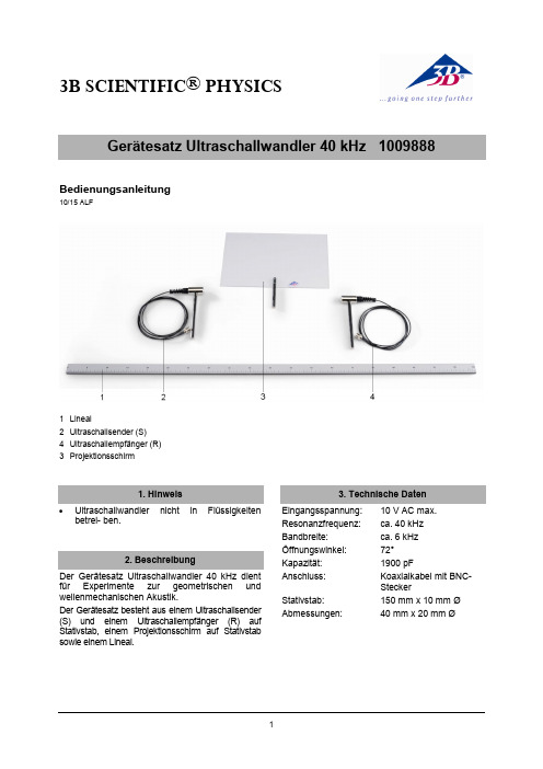
3B SCIENTIFIC ® PHYSICS1Bedienungsanleitung10/15 ALF1 Lineal2 Ultraschallsender (S) 4 Ultraschallempfänger (R)3ProjektionsschirmUltraschallwandler nicht in Flüssigkeitenbetrei- ben.Der Gerätesatz Ultraschallwandler 40 kHz dient für Experimente zur geometrischen und wellenmechanischen Akustik.Der Gerätesatz besteht aus einem Ultraschallsender (S) und einem Ultraschallempfänger (R) auf Stativstab, einem Projektionsschirm auf Stativstabsowie einem Lineal.Eingangsspannung: 10 V AC max. Resonanzfrequenz: ca. 40 kHz Bandbreite:ca. 6 kHz Öffnungswinkel: 72°Kapazität: 1900 pFAnschluss: Koaxialkabel mit BNC-SteckerStativstab:150 mm x 10 mm Ø Abmessungen: 40 mm x 20 mm Ø3B Scientific GmbH ▪ Rudorffweg 8 ▪ 21031 Hamburg ▪ Deutschland ▪ Technische Änderungen vorbehalten © Copyright 2015 3B Scientific GmbH1 Funktionsgenerator FG 100 @230 V 1009957 oder1 Funktionsgenerator FG 100 @115 V 1009956 1 Analog-Oszilloskop 2x30 MHz 1002727 3 Tonnenfuß, 0,5 kg 1001046 1 HF-Kabel 1002746 1 T-Stück, BNC1002752 1 Adapter BNC-Buchse/4-mm-Stecker 10027515.1 Einstellen der Resonanzfrequenz∙ Ultraschallsender und Ultraschallempfängerin kurzem Abstand gegenüber stellen.∙Den Sender an den Ausgang des Funktionsgenerators anschließen und eine Frequenz von 40 kHz einstellen.∙ Den Empfänger an das Oszilloskop anschließen.∙Empfängersignal beobachten und durch Feineinstellung der Frequenz die Signal- amplitude maximieren.5.2 Experimentierbeispiel∙ Ultraschallsender und Ultraschallempfängernebeneinander vor den Projektionsschirm aufstellen.∙ Den Sender an den Ausgang desFunktionsgenerators anschließen und die Resonanzfrequenz einstellen (siehe 5.1).∙ Den Empfänger mit dem Oszilloskop ver-binden.∙ Projektionsschirm verschieben und Phasen-differenz der Signale beobachten.Fig. 1 Experimenteller Aufbau zum Einstellen der ResonanzfrequenzFig. 2 Experimenteller Aufbau zur Reflektion der Ultraschallwellen am Projektionsschirm。

frag跟踪原文英文版

Robust Fragments-based Tracking using the Integral HistogramAmit Adam and Ehud RivlinDept.of Computer Science Technion-Israel Institute of TechnologyHaifa32000,Israel{amita,ehudr}@cs.technion.ac.ilIlan ShimshoniDept.of Management Information SystemsHaifa UniversityHaifa31905,Israel{ishimshoni}@mis.haifa.ac.ilAbstractWe present a novel algorithm(which we call“Frag-Track”)for tracking an object in a video sequence.The template object is represented by multiple image fragments or patches.The patches are arbitrary and are not based on an object model(in contrast with traditional use of model-based parts e.g.limbs and torso in human tracking).Every patch votes on the possible positions and scales of the ob-ject in the current frame,by comparing its histogram with the corresponding image patch histogram.We then mini-mize a robust statistic in order to combine the vote maps of the multiple patches.A key tool enabling the application of our algorithm to tracking is the integral histogram data structure[18].Its use allows to extract histograms of multiple rectangular re-gions in the image in a very efﬁcient manner.Our algorithm overcomes several difﬁculties which can-not be handled by traditional histogram-based algorithms [8,6].First,by robustly combining multiple patch votes,we are able to handle partial occlusions or pose change.Sec-ond,the geometric relations between the template patches allow us to take into account the spatial distribution of the pixel intensities-information which is lost in traditional histogram-based algorithms.Third,as noted by[18],track-ing large targets has the same computational cost as track-ing small targets.We present extensive experimental results on challenging sequences,which demonstrate the robust tracking achieved by our algorithm(even with the use of only gray-scale(non-color)information).1.IntroductionTracking is an important subject in computer vision with a wide range of applications-some of which are surveil-lance,activity analysis,classiﬁcation and recognition from motion and human-computer interfaces.The three main categories into which most algorithms fall are feature-based tracking(e.g.[3]),contour-based tracking(e.g.[15])and region-based tracking(e.g[13]).In the region-based cate-gory,modeling of the region’s content by a histogram or by other non-parametric descriptions(e.g.kernel-density esti-mate)have become very popular in recent years.In particu-lar,one of the most inﬂuential approaches is the mean-shift approach[8,6].With the experience gained by using histograms and the mean shift approach,some difﬁculties have been studied in recent years.One issue is the local basin of convergence that the mean shift algorithm has.Recently in[22]the au-thors describe a method for converging to the optimum from far-away starting points.A second issue,inherent in the use of histograms,is the loss of spatial information.This issue has been addressed by several works.In[26]the authors introduce a new sim-ilarity measure between the template and image regions, which replaces the original Bhattacharyya metric.This measure takes into account both the intensities and their position in the window.The measure is further computed efﬁciently by using the Fast Gauss Transform.In[12],the spatial information is taken into account by using“oriented kernels”-this approach is additionally shown to be useful for wide baseline matching.Recently,[4]has addressed this issue by adding the spatial mean and covariance of the pixel positions who contribute to a given bin in the histogram-naming this approach as“spatiograms”.A third issue which is not speciﬁcally addressed by these previous approaches is occlusions.The template model is global in nature and hence cannot handle well partial occlu-sions.In this work we address the latter two issues(spatial in-formation and occlusion)by using parts or fragments to rep-resent the template.Theﬁrst issue is addressed by efﬁcient exhaustive search which will be discussed later on.Given a template to be tracked,we represent it by multiple his-tograms of multiple rectangular sub regions(patches)of the template.By measuring histogram similarity with patchesof the target frame,we obtain a vote-map describing the possible positions of each patch in the target frame.We then combine the vote-maps in a robust manner.Spatial in-formation is not lost due to the use of spatial relationships between patches.Occlusions result in some of the patches contributing outlier vote-maps.Due to our robust method for combining the vote maps,the combined estimate of the target’s position is still accurate.The use of parts or components is a well known tech-nique in the object recognition literature(see chapter23in [11]).Examples of works which use the spatial relation-ships between detections of object parts are[21,17,16,2]. In[24]the issue of choosing informative parts which con-tain the most information concerning the presence of an ob-ject class is discussed.A novel application of detecting un-usual events and salient features based on video and image patches has recently been described in[5].In tracking,the use of parts has usually been in the con-text of human body tracking where the parts are based on a model of the human body-see[23]for example.Re-cently,Hager,Dewan and Stewart[14](followed by Fan et al.[10])analyzed the use of multiple kernels for tracking. In these works the connection between the intensity struc-ture of the target,the possible transformations it can expe-rience between consecutive frames,and the kernel structure used for kernel tracking was analyzed.This analysis gives insight on the limitations of single-kernel tracking,and on the advantages of multiple-kernel tracking.The parts-based tracking algorithm described in this work differs from these and other previous works in a number of important issues:•Our algorithm is robust to partial occlusions-the works in[14,10]cannot handle occlusions due to the non-robust nature of the objective function.•Our algorithm allows the use of any metric for com-paring two histograms,and not just analytically-tractable ones such as the Bhattacharyya or the equiv-alent Matusita metrics.Speciﬁcally,by using non-componentwise metrics the effects of bin-quantization are reduced(see section2.1and Fig.3).•The spatial constraints are handled automatically in our algorithm by the voting mechanism.In contrast, in[10]these constraints have to be coded in(e.g.the ﬁxed length constraint).•The robust nature of our algorithm and the efﬁcient use of the integral histogram allows one to use the algo-rithm without giving too much thought on the choice of multiple patches/kernels.In contrast,in[14,10]the authors carefully chose a small number of multiple ker-nels for each speciﬁc sequence.•We present extensive experimental validation,on out-of-the-lab real sequences.We demonstrate good track-ing performance on these challenging scenarios,ob-tained with the use of only gray-scale information.Our algorithm requires the extraction of intensity or color histograms over a large number of sub-windows in the target image and in the object template.Recently Pork-ili[18]extended the integral image[25]data structure to an“integral histogram”data structure.Our algorithm ex-ploits this observation-a necessary step in order to be able to apply the algorithm for real time tracking tasks.We ex-tend the tracking application described in[18]by our use of parts,which is crucial in order to achieve robustness to occlusions.2.Patch TrackingGiven an object O and the current frame I,we wish to locate O in the ually O is represented by a tem-plate image T,and we wish toﬁnd the position and the scale of a region in I which is closest to the template T in some sense.Since we are dealing with tracking,we assume that we have a previous estimate of the position and scale,and we will search in the neighborhood of this estimate.For clarity,we will consider in the following only the search in position(x,y).Let(x0,y0)be the object position estimate from the pre-vious frame,and let r be our search radius.Let P T= (dx,dy,h,w)be a rectangular patch in the template,whose center is displaced(dx,dy)from the template center,and whose half width and height are w and h respectively.Let (x,y)be a hypothesis on the object’s position in the cur-rent frame.Then the patch P T deﬁnes a corresponding rectangular patch in the image P I;(x,y)whose center is at (x+dx,y+dy)and whose half width and height are w and h.Figure1describes this correspondence.Given the patch P T and the corresponding image patch P I;(x,y),the similarity between the patches is an indication of the validity of the hypothesis that the object is indeed located at(x,y).If d(Q,P)is some measure of similaritybetween patch Q and patch P,then we deﬁneV PT(x,y)=d(P I;(x,y),P T)(1) When(x,y)runs on the range of hypotheses,we getV PT (·,·)which is the vote map corresponding to the tem-plate patch P T.2.1.Patch Similarity MeasuresWe measure similarity between patches by comparing their gray-level or color histograms.This allows moreﬂexi-bility than the standard normalized correlation or SSD mea-sures.Although for a single patch we lose spatial informa-tion by considering only the histogram,our use of multiple patches and their spatial arrangement in the template com-pensates for this loss.There are a number of known methods for comparing the similarity of two histograms[9].The simplest methods compare the histograms by comparing corresponding bins. For example,one may use the chi-square statistic or sim-ply the norm of the difference between the two histograms when considered as two vectors.The Kolmogorov-Smirnov statistic compares histograms by building the cumulative distribution function(that is cu-mulative sum)of each histogram,and comparing these two functions.The advantage over bin-wise methods is smooth-ing of nearby bin differences due to the quantization of mea-surements into bins.A more appealing approach is the Earth Mover’s Dis-tance(EMD)between two histograms,described in[20]. In this approach the actual dissimilarity between the bins themselves is also taken into account.The idea is to com-pute how much probability has to move between the various bins in order to transform theﬁrst histogram into the second. In doing so,bin dissimilarity is used:for example,in gray scale it costs more to move0.1probability from the[16,32) bin to the[128,144)bin,than to move it to the[32,47) bin.In theﬁrst case,the movement of probability is re-quired because of a true difference in the distributions,and in the second case it might be due simply to quantization errors.This is exactly the transportation problem of linear programming.In this problem the bases are always triangu-lar and therefore the problem may be solved efﬁciently.See [20]for more details and advantages of this approach.We have experimented with two similarity measures. Theﬁrst is the naive measure which treats the histograms as vectors and just computes the norm of their difference. The second is the EMD measure.For gray scale images, we used16bins.The EMD calculation is very fast and poses no problem.For color images,the number of bins is much larger(with only8bins per channel we get512bins). Therefore when using the EMD we took the K=10bins which obtained maximal counts,normalized them tounityPatch vote map − naive (dis)similarity Patch vote map − EMD (dis)similarity(a)(b)Figure3.V ote maps for the example patch using the the naive mea-sure and the EMD measure.The lower(darker)the vote-the more likely the position.Left(a)-naive measure.Right(b)-EMD.The EMD surface has a less blurred minimum,and is smoother at the same time.and then used the EMD.We used the original EMD code developed by Rubner[19].Figure2shows an example patch(we use gray scale in this example).We computed the patch vote map for all the locations around the patch center which are up to30pixels above or below and up to20pixels to the left or right.Fig-ure3shows the resulting vote maps when using the naive measure and the EMD measure.Note that in both measures the lower the value(darker in the image),the more simi-lar the histograms.The EMD surface is smoother and has a more distinct minimum than the surface obtained when using the naive measure.bining Vote MapsIn the last section we saw how to obtain a vote map V PT(·,·)for every template patch P T.The vote map gives a scalar score for every possible position(x,y)of the tar-get in the current frame I,given the information from patch P T.We now want to combine the vote maps obtained from all template patches.Basically we could sum the vote maps and look for the position which obtained the minimal sum(recall that our vote maps actually measure dissimilarity between patches). The drawback of this approach is that an occlusion affecting even a single patch may contribute a high value to the sum at the correct position,resulting in a wrong estimate.In other words,we would like to use a robust estimator which couldhandle outliers resulting from occluded patches or other rea-sons(e.g.partial pose change-for example a person turns his head).One way to make the sum robust to outliers is to bound the possible contribution of an outlierC(x,y)=PV P(x,y)V P(x,y)<TT V P(x,y)>=T(2)by some threshold T.If we adopt a probabilistic view ofthe measurement process-by transforming the vote mapto a likelihood map(e.g.by setting L P(x,y)=K∗exp−α∗V P(x,y))-then this method is equivalent to addinga uniform outlier density to the true(inlier)density.Min-imizing the value of C(·,·)is then equivalent to obtaininga maximum likelihood estimate of the position,but without letting an outlier take the likelihood down to0.However,we found that choosing the threshold T isnot very intuitive,and that the results are sensitive to this choice.A different approach is to use a LMedS-type es-timator.At each point(x,y)we order the obtained val-ues{V P(x,y)|patches P}and we choose the Q’th smallest score:C(x,y)=Q th value in the sorted set{V P(x,y)|patches P}(3) The parameter Q is much more intuitive:it should be the maximal number of patches that we always expect to yield inlier measurements.For example,if we think that we are guaranteed that occlusions will always leave at least a quar-ter of the target visible,than we will choose Q to be25%of the number of patches(to be precise-we assume that at least a quarter of the patches will be visible).The additional computational burden when using esti-mate(3)instead of(2)is not signiﬁcant(the number of patches is less than40).ing the Integral HistogramThe algorithm that we have described requires multiple extractions of histograms from multiple rectangular regions.We extract histograms for each template patch,and then we compare these histograms with those extracted from mul-tiple regions in the target image.The tool enabling this tobe done in real time,as required by tracking,is the integral histogram described in[18].The method is an extension of the integral image data structure described in[25].The integral image holds at the point(x,y)in the image the sum of all the pixels containedin the rectangular region deﬁned by the top-left corner ofthe image and the point(x,y).This image allows to com-pute the sum of the pixels on arbitrary rectangular regionsby considering the4integral image values at the cornersFigure4.outer partof the regionof the region-in other words in(very short)constant timeindependent of the size of the region.In order to extract histograms over arbitrary rectangu-lar regions,in the integral histogram we build for each binof the histogram an integral image counting the cumula-tive number of pixels falling into that bin.Then by access-ing these integral images we can immediately compute thenumber of pixels in a given region which fall into every bin,and hence we obtain the histogram of that rectangular re-gion.Once the integral histogram data structure is computed(with cost proportional to the image(or actually search re-gion)size times the number of bins),extraction of a his-togram over a region is very cheap.Therefore evaluatinga hypothesis on the current object’s position(and scale)isrelatively cheap-basically it is the cost of comparing twohistograms.As noted previously,a tracking application of the integralhistogram was suggested in[18].We extend that examplewith the parts-based approach.4.1.Weighting Pixel ContributionsAn important feature in the traditional mean shift algo-rithm is the use of a kernel function which assigns lowerweights to pixels which are further away from the target’scenter.These pixels are more likely to contain backgroundinformation or occluding objects,and hence their contribu-tion to the histogram is diminished.However,when usingthe integral histogram,it is not clear how one may includethis feature.The following discrete approximation scheme may beused instead of the more continuous kernel weighting(seeFigure4).If we want to extract a weighted histogram inthe rectangular region R,we may deﬁne an inner rectangleR1and subtract the integral histogram counts of R1from those of R to obtain the counts in the ring R−R1.Thesecounts and the R1counts may be weighted differently andcombined to give a weighted histogram on R.Of course,anadditional inner rectangle R2may be used and so forth.The additional cost is the access and arithmetic involvedwith4additional pixels for every added inner rectangle.Formedium and large targets this cost is negligible when com-pared to trying to weigh the pixels in a straightforward man-ner.4.2.ScaleAs noted in[25,18],an advantage of the integral im-age/histogram is that the computational cost for large re-gions is not higher than the cost for small regions.This makes our search for the proper scale of the target not harder than our search for the proper location.Just as a hypothesis on the position(x,y)of the object deﬁnes a correspondence between a template patch P T and an image patch P I;(x,y),if we add a scale s to the hypoth-esis,it is straightforward toﬁnd the corresponding image patch P I;(x,y,s):we just scale the displacement vector of the patch and its height and width by s.The cost of extract-ing the histogram for this larger(or smaller)image patch is the same as for the same-size patch.We have implemented the standard approach(suggested in[8]and adopted by e.g.[4])of enlarging and shrinking the template by10%,and choosing the position and scale which give the lowest score in(3).The next section will present some results obtained with this approach.We remark that as noted in[7],this method has some limitations.For example,if the object being tracked is uniform in color,then there is a tendency for the target to shrink.In the case of partial occlusions of the target,we are faced with an additional dilemma:suppose that a uniform colored target is partially occluded.We get a good score by shrinking the target and locating it around the non-occluded part.Due to our robust approach,we also get a reasonable score by keeping the target at the correct size and locating it at the correct position,which includes some occluded parts of the target.However,there is no guarantee that the correct explanation will yield a better score than the partial expla-nation.A full treatment of this problem is out of the scope of the current work.5.ResultsNote:The full video clips are available at the authors’websites.We now present our experimental results.The tracker was run on gray scale images and the histograms we used contained16bins.Note that the integral histogram data structure requires an image for every bin in the histogram, and therefore on color images the application can become quite memory-consuming.We used vertical and horizontal patches as shown in Fig-ure5.The vertical patches are of half the template height, and about one tenth of the template’s width.The horizon-tal patches are deﬁned in a similar manner.Over all we had around36patches(the number slightly varies with template size because of rounding to integer sizes).We note thatthis choice of patches was arbitrary-we just tried it and found it was good enough.In the discussion we return to this issue.The search radius was set to7pixels from the previous target position.The template wasﬁxed at theﬁrst frame and not updated during the sequence(more on this in the discussion).We used the25’th percent quantile for the value of Q in(3).These settings of the algorithm’s parameters wereﬁxed for all the sequences.Theﬁrst two sequences(“face”and“woman”)show the robustness to occlusions.For these sequences we manually marked the ground truth(everyﬁfth frame),and plotted the position error of our tracker and of the mean-shift tracker. In both cases our tracker was not affected by the occlusions, while the mean-shift tracker did drift away.Figures6and 7show the errors with respect to the ground truth.Figure8 shows the initial templates and a few frames from these se-quences.Note the last frame of the woman sequence(sec-ond row)where one can see an example of the use of spatial information(seeﬁgure caption also).We additionally note that we ran our tracker on these ex-amples with only a single patch containing the whole tem-plate,and it failed(this is actually the example tracker de-scribed in[18]).The next sequence-“living room”in Figure9-shows performance under partial pose change.When the tracked woman turns her head the mean shift tracker drifts,and then together with an occlusion it gets lost.Our tracker is robust to these interferences.In Figure10we present more samples from three more sequences.In these frames we marked only our tracker.The ﬁrst two sequences are from the CA VIAR database[1].The ﬁrst is an occlusion clip and the second shows target scale changes.The third sequence is again an occlusion clip.We bring it to demonstrate how our tracker uses spatial informa-tion(which is generally lost in histogram-based methods). Both persons have globally similar histograms(half dark and half bright).Our tracker“knows”that the bright pixels should be in the upper part of the target and therefore does not drift to the left person when the two persons are close.6.Discussion and ConclusionsIn this work we present a novel approach(“FragTrack”) to tracking.Our approach combines fragments-based repre-initial template frame 222frame 539frame 849initial template frame 66frame 134frame 456Figure 8.Occlusions -frames from “face”and “woman”sequences.Our tracker -solid red.Mean-shift tracker -dashed blue.Note in frame 456how the spatial information -bright in the upper part,dark in the lower part -helps our tracker.The mean-shift tracker which does not have this information chooses a region witha dark upper part and a bright lower part.initial template frame 29frame 141frame 209Figure 9.Pose change and occlusions -frames from “living room”sequence.Our tracker -solid red.Mean-shift tracker -dashed blue.40506070Position error w.r.t. ground truthn p i x e l s )our trackermean shift trackerground truth.Our tracker -solid red.Mean shift -dashed blue.Please see videos for additional impression sentation and voting known from the recognition literature,with the integral histogram tool.The result is a real time tracking algorithm which is robust to partial occlusions and 2530354045Position error w.r.t. ground truthn p i x e l s )our trackermean shift trackermarked ground truth.Our tracker -solid red.Mean shift -dashed blue.Please see videos for additional impressionpose changes.In contrast with other tracking works,our parts or frag-ments approach is model-free:the fragments are choseninitial template frame48frame82frame110initial template frame30frame100frame180initial template frame35frame65frame90Figure10.Additional examples.Theﬁrst two rows are from the CA VIAR database.No background subtraction/frame differencing was used.In the last row note again the use of spatial information-both persons have the same global histogram.arbitrarily and not by reference to a pre-determined parts-based description of the target(say limbs and torso in hu-man tracking,or eyes and nose in face tracking).Without the integral histogram’s efﬁcient data structure it would not have been possible to compute each fragment’s votes map.On the other hand,without using a fragments-based algorithm,robustness to partial occlusions or pose changes would not have been possible.We demonstrate the validity of our approach by accu-rate tracking of targets under partial occlusions and pose changes in several video clips.The tracking is achieved without any use of color information.There are several interesting issues for current and fu-ture work.Theﬁrst is the question of template updating. We want to avoid introduction of occluding objects into the template.The use of the various fragments’similarity scores may be useful towards meeting this goal.A second issue is the partial versus full explanation dilemma described earlier and in[7]when choosing scale. This dilemma is even more signiﬁcant under partial occlu-sions.Lastly,we may also consider disconnected rectangular fragments.It would be interesting toﬁnd a way to choose the most informative fragments[24]with respect to the tracking task.References[1]Caviar datasets available at/vision/caviar/caviardata1/.[2]S.Agarwal,A.Awan,and D.Roth.Learning to detect ob-jects in images via a sparse,part-based representation.IEEE Transactions on Pattern Analysis and Machine Intelligence, 20(11):1475–1490,2004.[3] D.Beymer,P.McLauchlan,B.Coifman,and J.Malik.Areal-time computer vision system for measuring trafﬁc pa-rameters.In Proc.IEEE Conf.on Computer Vision and Pat-tern Recognition(CVPR),1997.[4]S.Birchﬁeld and S.Rangarajan.Spatiograms vs.histogramsfor region based tracking.In Proc.IEEE Conf.on Computer Vision and Pattern Recognition(CVPR),2005.[5]O.Boiman and M.Irani.Detecting irregularities in imagesand video.In Proc.IEEE Int.Conf.on Computer Vision (ICCV),2005.[6]G.Bradski.Real time face and object tracking as a compo-nent of a perceptual user interface.In Proc.IEEE WACV, pages214–219,1998.[7]R.Collins.Mean shift blob tracking through scale space.InProc.IEEE Conf.on Computer Vision and Pattern Recogni-tion(CVPR),pages II:234–240,2003.[8] aniciu,R.Visvanathan,and P.Meer.Kernel basedobject tracking.IEEE Transactions on Pattern Analysis and Machine Intelligence,25(5):564–575,2003.[9]W.Conover.Practical Nonparamteric Statistics.Wiley,1998.[10]Z.Fan,Y.Wu,and M.Yang.Multiple collaborative kerneltracking.In Proc.IEEE Conf.on Computer Vision and Pat-tern Recognition(CVPR),2005.[11] D.Forsyth and puter Vision:A Modern Ap-proach.Prentice-Hall,2001.[12] B.Georgescu and P.Meer.Point matching under large imagedeformations and illumination changes.IEEE Transactions on Pattern Analysis and Machine Intelligence,26:674–689, 2004.[13]G.Hager and P.Belhumeur.Efﬁcient region tracking withparamteric models of geometry and illumination.IEEE Transactions on Pattern Analysis and Machine Intelligence, 20(10):1125–1139,1998.[14]G.Hager,M.Dewan,and C.Stewart.Multiple kernel track-ing with ssd.In Proc.IEEE Conf.on Computer Vision and Pattern Recognition(CVPR),2004.[15]M.Isard and A.Blake.Condensation:Conditional densitypropagation for visual tracking.Int.Journal of Computer Vision(IJCV),29(1):5–28,1998.[16]K.Mikolajczyk,C.Schmid,and A.Zisserman.Humandetection based on a probabilistic assembly of robust part detectors.In Proc.Eurpoean Conf.on Computer Vision (ECCV),2004.[17] A.Mohan, C.Papageorgiou,and T.Poggio.Example-based object detection in images by components.IEEE Transactions on Pattern Analysis and Machine Intelligence, 23(4):349–361,2001.[18] F.Porkili.Integral histogram:A fast way to extract his-tograms in cartesian spaces.In Proc.IEEE Conf.on Com-puter Vision and Pattern Recognition(CVPR),2005.[19]Y.Rubner.Code available at /∼rubner/.[20]Y.Rubner,C.Tomasi,and L.Guibas.The earth mover’sdistance as a metric for image retrieval.Int.Journal of Com-puter Vision(IJCV),40(2):91–121,2000.[21] C.Schmid and R.Mohr.Local gray-value invariants for im-age retrieval.IEEE Transactions on Pattern Analysis and Machine Intelligence,1997.[22] C.Shen,M.Brooks,and A.Hengel.Fast global kernel den-sity mode seeking with application to localisation and track-ing.In Proc.IEEE Int.Conf.on Computer Vision(ICCV), 2005.[23]L.Sigal et al.Tracking loose-limbed people.In Proc.IEEEConf.on Computer Vision and Pattern Recognition(CVPR), 2004.[24]S.Ullman,E.Sali,and M.Vidal-Naquet.A fragment-basedapproach to object representation and classiﬁcation.In Proc.IWVF4,LNCS2059,pages85–100,2001.[25]P.Viola and M.Jones.Robust real time object detection.In IEEE ICCV Workshop on Statistical and Computational Theories of Vision,2001.[26] C.Yang,R.Duraiswami,and L.Davis.Efﬁcient mean-shifttracking via a new similarity measure.In Proc.IEEE Conf.on Computer Vision and Pattern Recognition(CVPR),2005.。

CS1.6服务器

cs1.6服务器架设来源:转发更新时间:2006-12-23 点击:1605次cs1.6服务器架设一、基本安装篇1、建立服务器的带宽和机器配置1.6服务器对对带宽和机器配置的要求比1.5高一些，我在ADSL上通过浩方平台建立1.5服务器，可以在本机上进行游戏，但是1.6出现明显的停顿，无法流畅的游戏，即使机器配置很高也不能彻底解决，相信带宽是最大的瓶颈。

因此，使用ADSL或者机器配置一般的cser建议不要在本机上建立服务器，用lan的cser在本机上建立服务器效果也不会太理想（除非你只想提供一个服务器，过一把OP 的瘾，呵呵）。

2、1.6服务器版本我收集有6个版本的cs1.6，通过试用，个人认为esai2738经典版是最好的，只有200M，同时包括了建立服务器的必要组件，用来游戏与经典版建立的服务器能够很好的兼容。

下载地址：bt种子下载3、下载完毕后，点击桌面的快捷方式‘Cs1.6服务器’，自己的服务器就开始工作了，就这么简单？！呵呵。

不要只扔西红柿，再来几个鸡蛋，鸡蛋西红柿：）这只是第一步。

看看下边吧：二、设置篇1、右键打开桌面快捷方式的属性：×:\Cs1.6中文版\hlds.exe -game cstrike -port 27016 +maxplayers 16 +map de_dust2 -console +localinfo mm_gamedll dlls/hldsmp.dll其中27016为服务器端口，可以进行修改；maxplayers 16为最大人数，可以自由变更，别超过32；开始地图de_dust2可以更换成你喜欢的地图；+localinfo mm_gamedll dlls/hldsmp.dll指你的游戏用哪个dll启动（很多人反映没有新特性，就是由于你的dll没设置好）其他的参数建议不要更改。

2、反作弊软件的选择很多自己建立了服务器的cser会发现无法进入游戏，或者进入后很快被踢出，我在开始建立服务器的时候也遇到了类似问题。

LTE CS fallback技术及测试例介绍

城市覆盖优化
总结词
通过LTE CS Fallback技术，城市覆盖优化得以实现，提高了网络质量和用户满意度。
详细描述
在城市环境中，由于建筑物密集、人口众多等因素，网络覆盖常常面临挑战。LTE CS Fallback技术通过将用户回落到CS域，确保在网络信号不佳时仍能保持通话连续性和语音质量，从而优化了城市覆盖。
安全与隐私保护的挑战
数据安全与隐私保护
随着LTE CS Fallback技术的广泛应用，数据安全和隐私保护成为重要挑战。需要采取有效的安全措施和技术手段，保护用户数据和隐私不被泄露或滥用。
网络安全防护
针对LTE CS Fallback网络的安全威胁和攻击，需要建立完善的网络安全防护体系，提高网络的安全性和可靠性，确保用户通信的顺利进行。
农村覆盖增强
总结词
LTE CS Fallback技术在农村覆盖增强方面发挥了重要作用，提高了网络信号的覆盖范围和稳定性。
详细描述
在农村地区，由于地形复杂、基站分布稀疏，网络覆盖常常成为问题。LTE CS Fallback技术通过合理利用网络资源，将用户回落到CS域，从而扩大了网络信号的覆盖范围，提高了信号的稳定性，使用户在农村地区也能享受到稳定的语音和数据服务。
当用户在LTE网络中发起或接收语音呼叫时，如果LTE网络无法提供足够的覆盖或质量，LTE CS Fallback机制将触发，将用户自动切换到CS域网络。
切换过程由移动管理实体（MME）和移动交换中心（MSC）之间的交互完成，无需用户干预。
技术优势与局限性
技术优势
LTE CS Fallback技术能够提供连续的语音服务，避免用户在通话过程中因网络切换而导致的通话中断。此外，该技术还能提高运营商对语音服务的控制力和灵活性。

化学反应工程英文课件Chapter 8

化学反应工程
Chapter 8 Potpourri of Multiple Reactions
Chapter 7 considered reactions in parallel. These
are reactions where the product does not react further. This chapter considers all sorts of reactions where the product formed may react further. Here are some examples:
化学反应工程
In the al‟ternative (二中择一的) way (shown in Fig. 8.2) of treating A, a small fraction of the beaker‟s contents is continuously removed, ir„radiated, and returned to the beaker. Although the total absorption rate is the same in the two cases, the intensity of radiation received by the removed fluid is greater, and it could well be, if the flow rate is not too high, that the fluid being irradiated reacts e‟ssentially to completion. In this case, then, A is removed and S is returned to the beaker. So, as time passes the concentration of A slowly decreases in the beaker, S rises, while R is absent (缺席的). This progressive change is shown in Fig.8.2.

Maxwell'sches Rad Auslo

3B SCIENTIFIC ® PHYSICSAuslösevorrichtung für Maxwell’sches Rad 1018075Bedienungsanleitung01/15 SD/UD1 Auslöser2 Haltestift3 Befestigungsschraube 44-mm-Sicherheitsbuchsen (Ausgang)1. SicherheitshinweiseDie Auslösevorrichtung entspricht den Sicher-heitsbestimmungen für elektrische Mess-, Steu-er-, Regel- und Laborgeräte nach DIN EN 61010 Teil 1. Sie ist für den Betrieb in trockenen Räu-men vorgesehen, die für elektrische Betriebsmit-tel geeignet sind.Bei bestimmungsgemäßem Gebrauch ist der sichere Betrieb des Gerätes gewährleistet. Die Sicherheit ist jedoch nicht garantiert, wenn das Gerät unsachgemäß bedient oder unachtsam behandelt wird.Wenn anzunehmen ist, dass ein gefahrloser Betrieb nicht mehr möglich ist (z.B. bei sichtba-ren Schäden), ist das Gerät unverzüglich außer Betrieb zu setzen.∙ Gerät nur in trockenen Räumen benutzen. ∙ Maximale Anschlussleistung von 25 V und0,25 A beachten.2. Technische DatenAnschlüsse: 4-mm-Sicherheitsbuchsen(Ausgang)Befestigung:2 Durchführungen (horizon-tal/vertikal) für Stativstangen 10 mm Ø mit Befestigungs-schraubeAbmessungen: 60 x 50 x 45 mm³ Masse: 250g3. BeschreibungDie Auslösevorrichtung dient dem Auslösen eines definierten Starts des Maxwell’schen Ra-des 1000790. Sie kann über die horizontale oder vertikale Durchführung mit Hilfe einer Be-festigungsschraube an Stativstangen mit 10 mm Durchmesser befestigt werden. Sie ist zum An-schluss an den Starteingang eines Digitalzäh-lers mit 4-mm-Sicherheitsbuchsen ausgestattet. Die Auslösevorrichtung arretiert mit Hilfe des Haltestiftes das Maxwell’sche Rad in der Start-position. Die Schalterstellung ist im arretiertenZustand wie auf dem Gehäuse aufgedruckt. Bei Betätigung des Auslösers werden die Kontakte umgeschaltet, das Rad wird freigegeben und gleichzeitig die Zeitmessung gestartet.4. Aufbewahrung, Reinigung, Entsorgung ∙Gerät an einem sauberen, trockenen und staubfreien Platz aufbewahren.∙Zur Reinigung keine aggressiven Reiniger oder Lösungsmittel verwenden.∙Zum Reinigen ein weiches, feuchtes Tuch benutzen.∙Die Verpackung ist bei den örtlichen Recyc-lingstellen zu entsorgen.∙Sofern das Gerät selbst verschrottetwerden soll, so gehörtdieses nicht in dennormalen Hausmüll,sondern ist in den da-für vorgesehenenElektroschrott-Contai-nernzu entsorgen. Essind die lokalen Vor-schriften einzuhalten.5. Bedienung / BeispielexperimentAbhängigkeit der Fallhöhe h vom Quadrat der Fallzeit t2 des Maxwell’schen RadesBenötigte Geräte:1 Maxwell’sches Rad 10007901 Stativfuß H-Form 10010422 Stativstange, 1000 mm 1002936 4 Universalmuffe 1002830 1 Stativstange 280 mm, 10 mm Ø 1012848 1 Auslösevorrichtung fürMaxwell’sches Rad 1018075 1 Lichtschranke 1000563 1 Digitalzähler mit Schnittstelle(@230 V) 1003123 oder1 Digitalzähler mit Schnittstelle(@115 V) 1003122 1 Satz 3 Sicherheitsexperimentier-kabel zum Freier-Fall-Gerät 1002848 1 Höhenmaßstab, 1m 1000743 1 Satz Zeiger für Maßstäbe 1006494 1 Tonnenfuß, 900 g 1001045 ∙Experiment gemäß Fig. 1 aufbauen.∙Achse des abgewickelten Maxwell’schen Rades mit Hilfe der beiden Einstellschrauben horizontal ausrichten.∙Lichtschranke so ausrichten, dass der Sen-sor von der Achse des Rades unterbrochen wird und nicht z.B. von einer Achsendkappe.Darauf achten, dass eine Kollision des Ra-des mit der Lichtschranke vermieden wird. ∙Lichtschranke an die mini-DIN8-Buchse PHOTO/MIC des Zählereingangs B an-schließen.∙Auslösevorrichtung an horizontaler Stativ-stange 280 mm so befestigen, dass der Hal-testift mittig über dem Rad steht und auf die Achse des Rades zeigt.∙Rote Buchse des Zählereingangs A mit Hilfe des grünen Sicherheitsexperimentierkabels 150 cm mit gelber Buchse der Auslösevor-richtung verbinden. Schwarzes und rotes Si-cherheitsexperimentierkabel 75 cm ineinan-der stecken und schwarze Buchse des Zäh-lereingangs A mit schwarzer Buchse der Auslösevorrichtung verbinden.∙Auslösevorrichtung vorspannen. Dazu Aus-löser mit dem Daumen bis zum Anschlag eindrücken und Rändelschraube mit dem Zeigefinger leicht gegen Uhrzeigersinn dre-hen.∙Maxwell’sches Rad vorsichtig aufwickeln und mit Hilfe des Haltestifts an der vorge-spannten Auslösevorrichtung arretieren.∙Beim Arretieren des Rades dieses nicht durch den Haltestift aus seiner Ruhelage verschieben. Ggf. die horizontale Ausrich-tung des Rades nachjustieren.∙Höhenmaßstab im Tonnenfuß wie in Fig. 1 gezeigt aufstellen.∙Oberen Zeiger so verschieben, dass er die Position der Achse des arretierten Rades anzeigt.∙Unteren Zeiger so verschieben, dass er die Position des Sensors in der Lichtschranke anzeigt.∙Am Zähler mit dem Druckknopf ‘FUNCTION’ die Betriebsart ‘START A – STOP B’ wäh-len.∙Auslösevorrichtung betätigen. Dazu Auslö-ser leicht eindrücken, Rändelschraube mit dem Zeigefinger leicht im Uhrzeigersinn drehen und Auslöser loslassen.Das Rad wird freigegeben und der Zähler startet gleichzeitig die Zeitmessung. Sobald die Achse des Rades die Lichtschranke unterbricht, wird die Messung automatisch gestoppt. Die Fallzeit wird in s oder ms angezeigt.∙Fallzeit t am Zähler und Fallhöhe h als Differenz der beiden Zeigerpositionen am Höhenmaßstab ablesen. Werte notieren.∙Messung für unterschiedliche Fallzeiten und Fallhöhen, d.h. unterschiedliche Positionen von Lichtschranke und unterem Zeiger des Höhenmaßstabs wiederholen.∙Fallhöhe h in Abhängigkeit des Quadrates der Fallzeit t2 auftragen (Fig. 2). Gemäß221()21gh t tIM r=⋅⋅+⋅g: ErdbeschleunigungI: Trägheitsmoment des RadesM: Masse des Radesr: Radius der Achseergibt sich ein linearer Zusammenhang. Aus der Steigung einer Ausgleichsgeraden an die Messpunkte kann entweder I bestimmt werden, wenn g, M und r bekannt sind, oder g, wenn I = 1/2·M·R2 (R: Radius des Rades), M und r bekannt sind.Fig. 1: Experimenteller Aufbau.3B Scientific GmbH ▪ Rudorffweg 8 ▪ 21031 Hamburg ▪ Deutschland ▪ Technische Änderungen vorbehalten0,00,20,40,60,8h / mt 2/ s2Fig. 2: h (t 2 )-Diagramm.。

通信工程CS Fallback技术探讨

通信工程CS Fallback技术探讨CS Fallback技术最初是在LTE技术中应用的，其主要作用是在LTE网络不可用时，可以实现用户回到2G/3G网络进行通信。

在移动通信领域，网络覆盖和服务质量是至关重要的因素。

为此，通信工程师不断探索新的技术，以提供更好的服务。

本文就对CS Fallback技术进行探讨。

首先，我们需要理解什么是LTE(Network Long-term Evolution)网络。

它是第4代移动通信系统的最新标准，具有更高的数据传输速率、更低的延迟及更好的服务质量等特点。

由于其覆盖范围有限，且不同运营商的LTE网络也可能存在差异，所以在某些情况下用户可能无法接入LTE网络，比如在山区或者隧道内等环境，这时就需要借助CS Fallback技术实现回退到2G/3G网络进行通信。

其实，CS Fallback技术的原理比较简单。

当用户在LTE网络下拨打电话时，若所在区域没有LTE信号覆盖，那么手机将自动切换到2G/3G网络，使用CDMA/GSM网络进行通信，以保证通话质量。

在用户通话结束后，手机又会自动回到LTE网络。

当然，在回落到2G/3G网络时，用户的数据传输速率会变慢，但通话质量会有所提高。

除了通话外，CS Fallback技术也适用于其他业务，比如短信、彩信和数据传输等。

同样地，在用户进行数据传输时，如果当前所在区域无法接入LTE网络，那么移动设备也将自动回落到2G/3G网络。

实际上，CS Fallback技术并不仅仅是简单地回落到2G/3G网络而已。

它还需要考虑到设备与网络的互通性，需要对两种不同的技术进行协调和转换。

比如，在从LTE到2G/3G的切换过程中，需要对网络频段进行转换。

这对于通信工程师的要求也更高，需要根据不同的移动设备以及运营商需求进行技术定制，保证用户的使用体验。

总之，CS Fallback技术是一种可靠的技术工具，为移动通信领域的用户提供越来越优质的服务。

计算机组成与设计-410

CS61C L16 Floating Point II (10) Garcia, Fall 2006 © UCB
Decoding Example (7/7) Before Hex: • After C code (Mapping below)
00001025hex 0005402Ahex 11000003hex 00441020hex 20A5FFFFhex 08100001hex
ห้องสมุดไป่ตู้
Review • Reserve exponents, significands:
Exponent 0 0 1-254 255 255 Significand 0 nonzero anything 0 nonzero Object 0 Denorm +/- fl. pt. # +/- ∞ NaN
• 4 rounding modes (default: unbiased)
True Assembly Language (1/3)
• Pseudoinstruction: A MIPS instruction that doesn’t turn directly into a machine language instruction, but into other MIPS instructions • What happens with pseudo-instructions?
• Look at opcode: 0 means R-Format, 2 or 3 mean J-Format, otherwise I-Format.
• Next step: separation of fields
CS61C L16 Floating Point II (7) Garcia, Fall 2006 © UCB

Sprecher + Schuh CS8微型闸关系系统说明说明书

GC S 8 C o n t r o l R e l a y sG17visit /ecatalog for pricing and the most up to date informationDespite increasing complexity, control systems and installations must become increasingly compact. And the CS8 Miniature Relay System packs maxi-mum performance into minimum space.Small but ruggedSprecher + Schuh has subjected this relay series to monitored endurance tests that demonstrate their ruggedness. Under normal duty, CS8 contacts have an elec-trical life of 700,000 operations, while the AC magnet system has a mechanical life of 15,000,000 operations.The coil is designed for absolute under-voltage reliability. Undervoltages that do not cause the contactor to close can be withstood indefinitely without damage.The body of the device is sturdy as well. The front housing, containing the phase partitions and screwdriver guides, is manufactured in one piece. Front and rear housing are then joint fitted together.Superior Contact ReliabilityThe standard CS8 base relay and aux-iliary contacts are bifurcated H-bridge design which divides each movable contact into two sections at the tip of thespanner which provides a higher degree of reliability for low signal applications. Perfect fit for PLC and other electronic circuits operate at signals as low as 15V @ 2mA.Mechanically linked contacts for safetyThe CS8 control relay are the perfectchoice for fail-safe control circuits tomeet mechanically linked performanceper IEC 60947-4-1. Mechanically linkedis an interlock contact design that main-tains minimum 0.5mm clearance which prevents the NC contact from reclosing if the NO contact is welded when in op-eration. This feature applies to CS8 base relays with AC & DC coils; base relaysand add-on auxiliaries for DC coils only.CS8 front mount auxiliaries arepositive guidanceCS8 Industrial Control RelaysThe miniature relay system with bigadvantagesAccessories require no additional panel spaceThe entire CS8 system is logicallyengineered. Auxiliary contact blocks are modular and snap-on without increasing the CS8’s original width of 45mm. Also, due to its sideways switching movement, the basic relay has the same low profile whether an AC or DC operating magnet is used. This permits the use of enclo-sures with shallow mounting depths. Once the CS8 is installed, all auxiliary contact blocks can be snapped on or removed without changing any existing wiring.Auxiliary components provide flexibilityCS8 auxiliary components allow you to convert the basic four pole relay up to an 8 pole relay.Effortless installationCS8 relays are DIN-rail mountable for instant installation and modifica-tion. Fittings are also included for base mounting. All terminals are clearlymarked and shipped in the open positionfor installation with either manual orpower screwdrivers. Using self-adhesivelabels, or plastic clip-on tags.The entire line is cULus Listed and CE Certified and offers finger and back of hand protection to the strictest interna-tional standards.C S 8 C o n t r o l R e l a y sG18visit /ecatalog for pricing and the most up to date informationDiscount Schedule B7CS8 RelayContact Arrangement andNumberingContacts AC OperationDC OperationNONCCatalog NumberCatalog Number4CS8-40E-✱CS8C-40E-✱31CS8-31Z-✱CS8C-31Z-✱22CS8-22Z-✱CS8C-22Z-✱1+1EM 1+1LBCS8-L22Z-✱CS8C-L22Z-✱CS8 Complete Assemblies - 4 Pole➊ The coil codes shown are for the most commonly stocked items. Contact yourSprecher + Schuh representative to determine if other voltages are on-hand or can be specially ordered in quantity.➋ Integrated diode surge suppressor coils available. Order coil code 24DD. For example CS8C-22Z-24D becomes CS8C-22Z-24DD. List price adder applies.➌ Contacts are bifurcated (H-bridge) with a minimum current rating of 2mA @ 15V.❹ The European Community has agreed that 400V is the nominal voltage in lieu of 380V. Use this code when 380V is required.➎ Use this code for 575V applications.StandardCircuit VoltageMake (Amps/VA)Break (Amps/VA)Continuous AmpsB600120AC 240AC 480AC 600AC 30A/3600VA 15A/3600VA 7.5A/3600VA 6A/3600VA 3.0A/360VA 1.5A/360VA 0.75A/360VA 0.60A/360VA 10Q600125DC 250DC 301-600DC0.55A/69VA 0.27A/69VA 0.1A/69VA0.55A/69VA 0.27A/69VA 0.1A/69VA2.5Contact Ratings (Per UL508/NEMA B600 & Q600) ➌Mechanical Link• B ase relay meets IEC 60947-5-1.See page G20 for additional information.GC S 8 C o n t r o l R e l a y sG19visit /ecatalog for pricing and the most up to date informationDiscount Schedule B7➊ Auxiliary contact ratings per UL 508/NEMA (B600/Q600). Contacts are bifur-cated (H-bridge) with a minimum current rating of 15V@2mA.➋ CS8 relays with 24 VDC coils can be special ordered with integrated diodes (built-in) rather than applying CRD8 to the coil terminals.➌ Base relay with add-on auxiliaries meet mechanically linked IEC 60947-5-1 for CS8 DC coil versions only. See page G20 for additional information.Auxiliary Contact BlocksNO NC Contact Arrangement Catalog Number 2-PoleTypical auxiliary contact block4-Pole11CS8-P11E2CS8-P02E20CS8-P20E22CS8-P22Z31CS8-P31Z13CS8-P13E4CS8-P04E40CS8-P40EAuxiliary Contact Blocks (2 & 4 Pole) ➊➌Auxiliary Contact BlocksNO NC Contact ArrangementCatalog Number 2-Pole Typical auxiliary contact block4-Pole11CA8-P112CA8-P022CA8-P2022CA8-P2231CA8-P3113CA8-P1304CA8-P044CA8-P40Miscellaneous AccessoriesC S 8 C o n t r o l R e l a y sG20visit /ecatalog for pricing and the most up to date informationDiscount Schedule B7Technical InformationCS8Auxiliary Contacts ElectricalContact Ratings — NEMA B600, Q600B600, Q600Contact Ratings — IEC AC-15 (solenoids, contactors)at rated voltage IEC 947, EN 60947NEMA B60024...120V [A]33230 (240V)[A]22400V [A] 1.2 1.2480...500V [A]11600 (690V)[A}0.60.6AC-12 (Rated thermal current)Ambient Temperature 40°C I th 24…690V [A]1010Ambient Temperature 60°C I th24 (240V)[A]66Low Level Signal Switching Contact design H-bridge bifurcatedH-bridge bifurcatedMinimum switching recommendation15V 2mA15V 2mAShort Circuit Protection Coordination Type 2acc. IEC 947-5-1Fuse gG [A]1010Switching DC-13 (Q600)1 pole24V [A] 2.3 2.348V [A]11110V [A]0.550.55125V [A]0.550.55220V [A]0.270.27250V [A]0.270.27400V [A]0.150.15440V [A]0.150.15600V [A]0.10.1Load Carrying Capacity according to UL/CSA Rated voltageAC [V]max. 600max. 600DC [V]max. 600max. 600Continuous rating (40ºC)AC [A]1010Switching CapacityAC [A]B600B600DC [A]Q600Q600Continuous rating (general purpose)300V [V]55600V[V]1010Resistance and Power Dissipation Main current circuit resistance, 1 pole [m Ω] 6.5 6.5Power dissipation I th , 4 poles [W] 2.6 2.6Total Power dissipation I th AC control, warm[W] 4.4 4.4DC control, warm[W]5.2 5.2Mechanically Linked Contacts and Mirror Contact PerformanceTypeCoilAdd-on Auxiliary ContactConforms to IECStatusCS8AC or DCNone 60947-5-1Mechanically linked within the base relayDC Yes 60947-5-1Mechanically linked within the base relay and with add-on auxiliary contactsACYes~Mechanically linked within the base relay onlyDefinitions• Mechanically linked contacts (IEC 60947-5-1 Annex L):• N.C. Auxiliary Contact will not re-close if a N.O. power pole welds.• N.O. Power Pole or Auxiliary Contact will not close if N.C. contact welds.• The term “Positive Guided” contacts is the same as mechanically linked.GC S 8 C o n t r o l R e l a y sG21visit /ecatalog for pricing and the most up to date informationDiscount Schedule B7CS8 RelaysMechanicalMechanical Life [Mil. Op]15Electrical LifeAC-15 (240V, 2A) AC Operations [Mil. Op]0.7WeightAC control [kg/lbs]0.16 (0.35)DC control [kg/lbs]0.2 (0.44)Fine strandedw/ ferrule 1 wire 2 wires[mm 2][mm 2]0.75...2.50.75...2.5Solid or coarse stranded1 wire2 wires[mm 2][mm 2]1…41...2.5 + 1…4Max. Wire Size ➊[AWG]18…12Tightening Torque[Nm] 1.2[lb-in]10.6Control CircuitOperating Voltage AC 50/60 Hz Pickup [x U s ]0.85…1.1Dropout [x U s ]0.2...0.75DCPickup[x U s ]0.8…1.1[x U s ]9,12,24,110V DC:0.7...1.25with protection circuit Dropout [x U s ]0.1...0.75Coil Consumption AC 50/60 Hz Inrush[VA/W]35/32Seal[VA/W]5/1.8DC Inrush/Seal [W]cold 3.0, warm 2.6Operating Times AC- 50/60 Hz Pickup Time[ms]15…40Dropout Time[ms]15…33With RC module Pickup Time [ms]15…28DC Pickup Time[ms]18…40Dropout Time[ms]6…12With Integ. diode Pickup Time [ms]8…12With External diode Pickup Time[ms]35 (50)CS8 RelaysGeneralRated Voltage Withstand U IEC 690V UL; CSA600V Rated Impulse Strength U imp 6 kVRated Voltage U e AC [V]24, 48, 120, 230, 400, 500, 600, 690DC[V]24, 48, 110, 220, 440V Rated Frequency AC 50/60 Hz, DC Ambient Temperature Storage–55...+80°C (–67...176°F)Operation at nominal current –25...+60°C (–13...140°F)At 85% rated operation current –25...+70ºC (–13... 158ºF)Resistance to Climatic Change40º C (104º F), 95% relative humidity,56 days23º C (73.4 º F), 83%/40 ºC (104 ºF),93%, 56 cyclesAltitude2000m M.S.L., per IEC 60947-4-1Type of Protection IP2XStandardsIEC/EN 60947-1, -5-1, -5-4; ➊ Pozidrive No.2 / Blade No.3 screwTechnical InformationC S 8 C o n t r o l R e l a y sG22visit /ecatalog for pricing and the most up to date informationDiscount Schedule B7。

蓝猫航天系列全集

01来自外太空的能量波 22我要驾驶02蓝猫的梦想 23肥仔生气了03我不会放弃的 24淘气出走04巴豆的加入 25竖立的硬币05淘气的飞行梦 26我们是朋友06会魔术的菲菲 27金星上的遭遇07找到航天飞船了 28火山喷发的木卫一08美丽瞬间 29水星遇险09交流 30咖喱的苦心10想飞的肥仔 31食物中的友谊11准备启航啦 32啦啦笑了12太空站 33寻找淘气13我们是真正的航天员啦 34遭遇彗星14昏迷的女孩 35冰球冥王星15交上新朋友 36会师冥王星16“竞选”船长 37突破龟速17蓝色光波拳 38啦啦晕倒了18登陆月球 39危险的宇宙射线19月球，我们来了 40无名舱里的能量石20我想开飞船 41丢失的能量石21美味的太空食物 42未知星云43神秘的蓝色星球 65我们被吸住了44啦啦的直觉 66找到能源45真和啦啦预料的一样 67寻访红巨星46遇险 68菲菲的离去47取能源 69菲菲的踪迹48飞向猎户座 70终获团圆49迫降第谷三 71不留情面的啦啦50飞船不见了 72菲菲的恶作剧51蘑菇山奇遇 73我要去黑洞52发现化石了 74进入黑洞了53怎么是你们 75都是我不好54有了新发现 76迫入巨人国55靠能量生长的蘑菇 77我们被喝进巨人肚子里了56舍己为人 78我们出来了57我们脱险了 79在巨人口袋里睡觉58飞向新地方 80淹没在美食中59初见陨冰 81他们也成了宠物60一波又起 82皇后的病好了61脱离困境 83啦啦冲进来了62啦啦的友情 84和好了63何去何从 85冰冻星球64一寻能源 86寒潮来了87初遇冰人 109你们搞错了88审问巴豆 110伟大的机器人89快逃出去呀 111迪卡和莱克的友谊90丽佳的眼泪 112救星迪卡91丽佳受伤了 113拯救机器人92菲菲治病 114危难的醒悟93争夺火焰果 115飞船着火了94神秘的波波 116向中子双星前进95我是清白的 117小布叽的计策96奇怪的红移现象 118冲出重围97波波的回忆 119会“唱歌”的黑洞98如何抉择 120梦游的巴豆99好朋友波波 121逃避追捕100巴豆VS千面人 122啦啦回到了过去101丽佳VS斯巴辛 123能量石还是散失了102冰冻解除 124回到现实103收到求救信号 125冲出黑洞104绿人警察局 126无名星球的召唤105机器人莱克 127神秘的大气层106初识迪卡和莱克 128奇怪的巨大图案107逃跑未遂 129大峡谷的秘密108菲菲报案 130失控的飞船131神秘的石像岛 153蓝猫的意外惊喜132北斗七星阵 154菲菲的机会133布叽的帮忙 155新官上任的菲菲134返回童心号 156矛盾升级135雪地脱险 157出师不利136快乐的小公主——啦啦 158菲菲的“英明”决策137啦啦的回忆 159母船危机138新啦啦的诞生 160蓝猫的失误139大闹石像阵 161终于找到了140勇闯神秘海 162好样的菲菲141智斗机器守卫 163咖喱的小心思142走出基地 164咖喱不开心了143失望的结局 165讨厌的啦啦姐姐144能量石在哪 166勇敢的咖喱145决定 167咖喱“受骗”146千万不能说 168咖喱生气了147猫猫？你需要休息 169自作聪明148大家在隐瞒什么 170伤心的咖喱149蓝猫的决定 171美丽的惊喜150蓝猫走了 172能量石的感应151银冕遇险 173遭遇火山爆发152误入暗星云 174啦啦想家了175狡猾的菲菲 197巴豆我们回去吧176我们一起共患难 198巴豆当上了队长177财宝财宝你在哪 199森林中的飞鱼178神奇的能量源 200摆脱吸人树179狐鱼大战 201大家分开了180可怕的蜘蛛 202可怕的食人球181我们是一家人 203巴豆的思想斗争182另一颗能量石 204巴豆的善意183危急时刻 205能量石到底在哪里184化险为夷 206巴豆独行185巴豆闯大祸了 207意外的礼物186对不起，是我的错 208再遇怪兽187让我帮忙吧 209我能行188怎么会这样 210寻找线索189巴豆的美味晚餐 211惊人的发现190自责的巴豆 212飞入陨石带191追查真相 213飞来的危险192水落石出 214淘气的挫折193失落的巴豆 215艰难的道歉194没有厨师的日子 216我该怎么办195落单的巴豆 217沉默的语言196森林遇险 218惊喜交加219飞出陨石带 241能量展现220心痒难耐的菲菲 242瑞奇的眼泪221好事多磨 243我们的友谊222沙尘暴 244菲菲的回忆223意外 245背后的故事224突如其来的灾难 246选拔比赛开始了225麻烦的巴豆 247绿森之死226哪来的饮水器 248成长227抓的是淘气 249终于找到原因了228菲菲找到钻石了 250误会229菲菲的钻石 251再起波澜230跑来跑去的能量石 252寻找探测器231钻石里的秘密 253飞行器被占了232消毒与隔离 254探测器风波233钻石友情 255踌躇234恐龙星球 256功亏一篑235初遇 257菲菲真的出走了236飞船里的故事 258你是我的小冤家237向毛毛虫驻地前进 259菲菲的计谋238寻找 260真的很想你们239毛毛虫基地 261菲菲的自尊240狭路相逢 262我们相信你263回家了 285奇异的星球264出乎意料 286菲菲开设科普班265神奇的能量石 287空忙一场266回到过去 288作坊里的故事267我要阻止自己 289我们是无辜的268一头雾水 290谷谷的想法269就是要驾驶 291巧入圣坛270淘气的劝告 292谷谷的飞行方法271这是一个梦吗 293飞船惊魂272受连累的巴豆 294不关他们的事273航向之争 295受困藤蔓274火星见真情 296绿色粽子275淘气不在小飞行器上 297误会难解276波折重重 298出状况的巴豆277淘气的任性 299再次被困278我的伙伴们 300难缠的藤蔓279食物真的是变出来的吗 301藤蔓里的秘密280手忙脚乱的淘气 302成功脱险281追赶淘气 303猫大哥的决定282啦啦的无奈 304再探圣坛283伙伴们，我爱你们 305盒子之谜284想飞的谷谷 306冰冻星球之新任务307再战千面人 329菲菲你在哪里308绅士斯巴辛的疯狂 330初闯总基地309终于拿到宝石了 331危险重重310途中遇险 332摆脱海盗311宝石合成了 333海盗王的真相312除去了隐患 334大义灭亲313我们也要飞起来 335神秘的机器人314遭遇海盗 336天空之港里的测试315狡猾的海盗 337我们不是玩具316紧急方案 338森的微笑317审问 339出乎意料318激战 340蓝猫被控制了319自投罗网 341遭遇追击320智取海盗小基地 342暗中帮助的青科321智救三人 343遭遇伏击322救治咖喱 344艰难的旅程323飞船保卫战 345猫大哥，我来了324你们抓不到我的 346重获自由325终于进了海盗秘密基地 347出人头地的机会来了326我们被骗了 348我们是实验品327被困钟楼 349智破机关328终于逃脱了 350别样的魔术师351一场误会 373奥茨玛，我们来了。

ngrams

• Models trained on 38 million words from the Wall Street Journal (WSJ) using a 19,979 word vocabulary. • Evaluate on a disjoint set of 1.5 million WSJ words.
Unknown Words
• How to handle words in the test corpus that did not occur in the training data, i.e. out of vocabulary (OOV) words? • Train a model that includes an explicit symbol for an unknown word (<UNK>).
Uses of Language Models
• Speech recognition
– “I ate a cherry” is a more likely sentence than “Eye eight uh Jerry”
• OCR & Handwriting recognition
– More probable sentences are more likely correct readings.
– Less realistic – Cheaper
• Verify at least once that intrinsic evaluation correlates with an extrinsic one.
Perplexity
• Measure of how well a model “fits” the test data. • Uses the probability that the model assigns to the test corpus. • Normalizes for the number of words in the test corpus and takes the inverse.

ae插件翻译（AEplug-intranslation）

ae插件翻译（AE plug-in translation）The first chapter, 55MM1.1 55mm Color Grad (color gradient)1.2 55mm Defocus (defocus)1.3 55mm Faux Flim (imitation film effect)1.4 55mm Fluorescent (Ying Guang)1.5 55mm Fog (FOG)1.6 55mm Infra-red (below red)1.7 55mm Mist (Bo Wu)1.8 55mm ND Grad (gradient)1.9 55mm Night Vision (night vision)1.10, 55mm, Selective, Soft, Focus (selective soft focus) 1.11 55mm Skin Smoother (flat outside surface)1.12 55mm Tint (partial color)1.13 55mm Warm/Cool (warm / cool)The second chapter, AEFlame (flame)The third chapter, Boris3.1 Boris Fire (flame effect)3.2 Boris FX 33.2.1 Boris Artist's Poster (Art Poster)3.2.2, Boris, Blur (fuzzy)3.2.3, Boris, Directional, Blur (directional blur)3.2.4, Boris, Gaussian, Blur (Gauss fuzzy)3.2.5, Boris, Unsharp, Mask (sharp mask)3.2.6, Boris, Brightness-Contrast (brightness contrast)3.2.7, Boris, Color, Balance (color balance)3.2.8, Boris, Color, Correction (color correction)3.2.9, Boris, Composite (synthesis)3.2.10, Boris, Correct, Selected, Color (modify the selected color)3.2.11, Boris, Hue-Sat-Lightness (hue saturation - brightness)3.2.12, Boris, Invert, Solarize (reverse exposure)3.2.13 Boris Levels Gamma (standard gamma value)3.2.14, Boris, MultiTone, Mix (multimodal mixing)3.2.15 Boris Posterize (multi tone color separation)3.2.16, Boris, RGB, Blend (RGB blend)3.2.17 Boris Tint-Tritone (replaced by three colors)3.2.18, Boris, Bulge (protruding)3.2.19, Boris, Displacement, Map (displacement mapping) 3.2.20, Boris, Fast, Flipper (auto flip)3.2.21, Boris, Polar, Displacement (bipolar replacement) 3.2.22, Boris, Ripple (ripple)3.2.23, Boris, Vector, Displacement (vector replacement) 3.2.24 Boris Wave (wave)3.2.25, Boris, Alpha, Process (Alpha channel processing) 3.2.26, Boris, Chroma, Key (chroma matting)3.2.27, Boris, Composite, Choker (suffocating synthesis) 3.2.28, Boris, Linear, Color, Key (linear color matting)3.2.29, Boris, Linear, Luma, Key (linear brightness matting)3.2.30, Boris, Make, Alpha, Key (make new Alpha channel)3.2.31, Boris, Matte, Choker (suffocating silhouette)3.2.32, Boris, Matte, Cleanup (clear Silhouettes)3.2.33, Boris, Two, Way, Key (two kinds of routes)3.2.34, Boris, Alpha, Spotlight (set the spotlight in Apha channels)3.2.35 Boris Edge Lighting (edge light)3.2.boris light sweep (36 扫光)3.2.37 boris reverse spotlight (相反的聚光灯)3.2.38 boris spotlight (聚光灯)3.2.39 boris 2d particles (二维粒子)3.2.40 boris 3d image (模拟三维图像破碎效果 shatter)3.2.41 boris cube (模拟三维立方体)3.2.42 boris cylinder (模拟三维圆柱体)3.2.43 boris binding (模拟三维效果)3.2.44 boris page turn (翻页)3.2.45 boris sphere (模拟三维球形)3.2.46 boris clouds (流动的云)3.2.47 boris noise map (噪点地图)3.2.48 boris alpha pixel noise (通道像素噪点)3.2.49 boris rgb edges (rgb边缘)3.2.50 boris rgb pixel noise (rgb像素噪声)3.2.51 boris scatterize (模拟毛玻璃的效果)3.2.52 boris spray paint noise (喷漆噪点)flat 3.2.53 boris 3d text (不支持中文扁平的三维字体 []) 3.2.54 boris 3d text (不支持中文三维字体 [])3.3 boris sync3d text (三维文字 3.3.1 bc)3.3.2 boost blend (推进混合 bc)3.3.3 bc burnt film (燃烧的电影)3.3.4 clouds (流动的云 bc)3.3.5 bc comet (彗星)3.3.6 bc composite (合成)3.3.7 binding (模拟三维效果 bc)3.3.8 bc fire (火)jitter bc (as specified in section 3.3.9 频谱曲线抖动) 3.3.10 looper (循环 bc)3.3.11 bc particle system (粒子系统)3.3.12 bc posterize time (相片时间)3.3.13 rain (下雨 bc)3.3.14 bc sequencer (音序器)3.3.15 snow (下雪 bc)3.3.16 sparks (火花 bc)3.3.17 stars (星星 bc)super blend (超级混合 3.3.18 bc)3.3.19 bc temporal blur (时间模糊)3.3.20 bc trails (轨迹)3.3.21 bc velocity remap (速度测试图)3.3.22 bc) (z空间1 z space)3.3.23 bc i (z) space z空间2)第4章 colormap (颜色地图)第5章 composite wizard5.1 cw composite color matcher (复合颜色匹配器)cw deluxe 5.2 (华丽的边缘查找器 edge finder)cw deluxe edge finder that is (5.3 华丽的边缘查找器ez) 5.4 (cw denoiser 放射状处理)cw edge blur (5.5 边缘模糊)cw edge blur is 5.6 (边缘模糊ez)5.7 cw matte feather (剪影羽化)this is (剪影羽化ez 5.8 cw matte feather)5.9 cw matte feather sharp (剪影羽化锐利) 5.10 cw miracle cleaner (alpha 通道清洁) 5.11 by cw - matter (重置剪影)5.12 cw smooth screen (光滑屏幕)5.13 cw spill killer (溢出杀手)5.14 cw spill killer ez (溢出杀手ez)5.15 cw super blur (超级模糊)5.16 cw super compound blur (超级混合模糊) 5.17 cw super rack focus (超级变焦)5.18 cw wire / rich zap (线框 / 钻探器) 5.19 cw zone hls (环绕hls)第7章 coycore7.1 cult effects 1.57.1.1 ce 3d glasses (三维眼睛)7.1.2 ce basic fill (基本填充)7.1.3 ce cell pattern (蜂房图案)7.1.4 ce change color hls (改变选择的颜色) 7.1.5 ce channeling (渠道)7.1.6 ce checker (棋盘格)7.1.7 ce circle (圆形)atmosphere ce color composite (颜色合成) 7.1.9 ce color link (颜色链接)7.1.10 ce color picker (颜色拾取)7.1.11 ce color solid (颜色固化)7.1.12 ce colorsquad (颜色四方格)7.1.13 ce difference (差异)7.1.14 ce fireup (火上)7.1.15 ce grid (网格)7.1.16 ce lightning (闪电)7.1.17 ce magnify (夸大效果)7.1.18 ce noise alpha (噪点通道)7.1.19 ce noise hls (噪点hls)7.1.20 ce noise hls auto (噪点hls自动)7.1.21 ce noise turbulent (骚乱的噪波)7.1.22 ce noise turbulent ii (骚乱的噪波2) 7.1.23 ce optics compensation (光学补偿) 7.1.24 ce paint (绘画)7.1.25 ce radial shadow (放射状的投影)7.1.26 ce the rough edges (让边缘变粗糙) 7.1.27 ce turbulent displace (汹涌的置换) 7.2 cult effects xtras7.2.1 ce set channel (设置通道)7.2.2 ce view channel (显示通道)第8章 digieffects8.1 digieffect aurorix v2.08.1.1 3d lighting 2 (光线彩色浮雕)8.1.2 agedfilm 2 (老电影的效果)8.1.3 bulgix 2 (类似于凸出的效果)8.1.4 chaotic noise 2 (混乱的噪波)8.1.5 chaotic rainbow 2 (混乱的五彩缤纷) 8.1.6 color spotlights 2 (彩色聚光灯) 8.1.7 earthquake 2 (震动)8.1.8 electrofield 2 (电磁感应)8.1.9 tinsel 2 (碎屑)8.1.10 fractal noise 2 (彩色不规则噪波2) 8.1.11 infinity warp 2 (无限扭曲)8.1.12 infinity zone 2 (无限环绕)8.1.13 interferix 2 (专用干扰图1)8.1.14 interpheroid 2 (专用干扰图2)8.1.15 interpheron 2 (专用干扰图2)8.1.16 lightzoom 2 (强光的纵深效果)8.1.17噪声2搅拌机（噪点搅拌机）2 8.1.18肥皂膜（皂膜）8.1.19射灯2（聚光灯）8.1.20奇怪星云2（奇异的星云）8.1.21蒂洛斯2（阵列）8.1.22湍流2（湍流）8.1.23 videolook 2（电视干扰信号）8.1.24 warpoid 2（拉伸效果）8.1.25 whirlix 2（旋转扭曲效果）8.1.26 woodmaker 2（木纹）8.2 digieffect berzerk V1.58.2.1暴雪（风雪）8.2.2 bumpmaker（制作凹凸贴图）8.2.3 contourist（轮廓线）8.2.4 Crystallizer（结晶器）8.2.5 cyclowarp（螺旋）- Edgex（边缘锐化）8.2.7雾虹（浓雾）8.2.8 GravityWell（重力旋涡）8.2.9激光（激光器）8.2.10新闻纸（新闻用纸）8.2.11 NightBloom（夜间华）8.2.12 OilPaint（油画）8.2.13珍珠（珍珠）8.2.14 perspectron（特殊的扭曲）8.2.15 ripploid（荡起的波纹）8.2.16 spintron（怪异的扭曲）8.2.18 StarField（飞舞的星星）8.2.19 StillNoise（静态噪点）8.2.20 vangoughist（美术笔触）8.3电影看filmres V1.18.3.1 DE CineLook（胶片调色）8.3.2 DE FilmDamage（胶片处理）8.4 cinemotion8.4.1 de自适应噪声（适应的噪点）8.4.2德带减速器（条带还原）8.4.3 de电影运动（运动电影）8.4.4 de粮食减速机（颗粒还原）8.4.5解交错叠减速器（交错产生器）8.4.6 de信箱（宽银幕产生器）8.4.7条款de选择HSB噪点（选择HSB噪点）8.4.8 de选择HSB色调分离（选择HSB多色调分色）8.4.9 de选择RGB噪音（选择RGB噪点）8.4.10 de选择RGB色调分离（选择RGB多色调分色）8.5 delerium8.5.1 de泡沫（泡沫）8.5.2 de相机抖动（摄像机抖动）8.5.3 DE Channel Delay（通道延迟）8.5.4 de警察模糊（优化模糊）8.5.5 de电弧（闪电）8.5.6仙尘（仙女的灰尘）8.5.7 de膜闪（影片闪烁）8.5.8脱火（火）8.5.9 de烟花（火焰发射器）8.5.10 de闪烁和频闪（闪光灯）8.5.11德流运动（流动）8.5.12 de雾厂（雾工厂）8.5.13 de框架梯度（画面渐变）8.5.14 DE Glower（炽热体）8.5.15 DE Grayscaler（灰度处理）8.5.16 de HLS取代（HLS置换）8.5。

CS8N65FA9H

WUX I CHINA RESOURCES HUAJING MICROELECTRONICS CO., LTD. Page 3 of 10 2011
Huajing Discrete Devices
○R CS8N65FA9H
Characteristics Curve：
100
70
Pd , Power Dissipation ,Watts
Test Conditions
VDS=15V, ID =4A VGS = 0V VDS = 25V f = 1.0MHz
Test Conditions
ID =8.0A VDD = 325V VGS = 10V RG = 12Ω
ID =8.0A VDD =325V VGS = 10V
Rating
Min. Typ. Max.
Huajing Discrete Devices
○R CS8N65FA9H
Source-Drain Diode Characteristics
Symbol
Parameter
IS
Continuous Source Current (Body Diode)
ISM
Maximum Pulsed Current (Body Diode)
5
10 15 20 25 30 35
Vds , Drain-to-Source Voltage , Volts
Figure 4 Typical Output Characteristics
50%
20%
10%
0.1
5%
PDM
t1 t2
Single pulse
2% 1%
NOTES： DUTY FACTOR ：D=t1/ t2 PEAK Tj=PDM*ZthJC*RthJC+TC

CS385

Quiz/test/Exam Lab Quiz 1.
ｈｔｔｐ：／／ｎｐｕｏｓｃ．ｎｐｕ．ｅｄｕ／ｓｔｕｄｅｎｔ／ｌｒｃ／Ｓｙｌｌａｂｕｓ／ＰｒｉｎｔＶｉｅｗ．ａｓｐｘ？ＣｏｕｒｓｅＯｆｆｅ．．．
２００５－８－３
ＮＰＵＣＡＭＳＥｎｇｉｎｅ
Objectives Instructive Coverage & Activities Assignments Others Week 3 Detail Weekly Objectives Instructive Coverage & Activities Assignments Others Week 4 Detail Weekly Objectives Instructive Coverage & Activities Assignments Others Week 5 Detail Weekly Objectives Instructive Coverage & Activities Assignments Others Week 6 Detail Weekly Objectives Instructive Coverage & Activities Assignments Quiz/test/Exam Others Week 7 Detail Weekly Objectives Instructive Coverage & Activities Assignments Others Week 8 Detail Weekly Objectives Instructive Coverage & Activities Assignments Process. Decisions, Test & Loops. 1) conditional statement if.....then...; 2) case switch, test statement, boolean constructs; 3) FOR, WHILE and UNTIL looping. Homework 7. Homework 6 due. Homework 5 due. Midterm (I) and ACL. Sed and AWK. I/O redirection and piping. Regular Expressions. Regular, full and extended expressions, grep command family. Homework 3. Homework 2 due. File and File System.

S CIENTIFIC PHYSI CS 1 Millisecond Counter 说明书

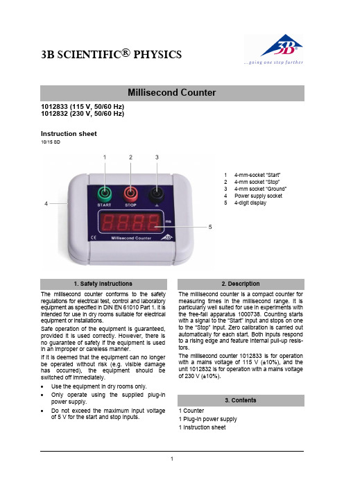
3B SCIENTIFIC ® PHYSICS11012833 (115 V, 50/60 Hz) 1012832 (230 V, 50/60 Hz)Instruction sheet10/15 SD1 4-mm-socket “Start”2 4-mm socket “Stop”3 4-mm socket “Ground”4 Power supply socket5 4-digit displayThe millisecond counter conforms to the safety regulations for electrical test, control and laboratory equipment as specified in DIN EN 61010 Part 1. It is intended for use in dry rooms suitable for electrical equipment or installations.Safe operation of the equipment is guaranteed, provided it is used correctly. However, there is no guarantee of safety if the equipment is used in an improper or careless manner.If it is deemed that the equipment can no longer be operated without risk (e.g. visible damage has occurred), the equipment should beswitched off immediately. ∙ Use the equipment in dry rooms only. ∙ Only operate using the supplied plug-in power supply.∙Do not exceed the maximum input voltage of 5 V for the start and stop inputs.The millisecond counter is a compact counter for measuring times in the millisecond range. It is particularly well suited for use in experiments with the free-fall apparatus1000738. Counting starts with a signal to the “Start” input and stops on one to the “Stop” input. Zero calibration is carried out automatically for each start. Both inputs respond to a rising edge and feature internal pull-up resis-tors.The millisecond counter 1012833 is for operation with a mains voltage of 115 V (±10%), and the unit 1012832 is for operation with a mains voltage of 230 V (±10%). 1 Counter1 Plug-in power supply 1 Instruction sheet2Inputs:Connectors:4-mm safety sockets Internal resistance “Start” input: 2.4 k Ω “Stop” inp ut: 5.6 k Ω Edges for “Start” and “Stop” inputs: RisingTrigger threshold for “Start” input: Low 0...0.5 V, high 1...5 V “Stop” input: Low 0...1 V, High 2...5 V Display: Display:4-digit LED display Measuring range: 1...9999 ms Resolution: 1 msPrecision: Quartz precision General data: Voltage supply: Plug-in power supply 12 V AC, 500 mADimensions: 100x75x35 mm³ approx Weight: 400 g approx. incl. plug-in power supply5.1 General operation ∙Connect a 12 V AC plug-in power to the millisecond counter (4).Connect both inputs (1 + 2) to ground (3). ∙Opening the “Start” input (1) (disconnecting the ground) starts the measurement.Measurement ceases as soon as the “Stop” input (2) is opened.The display will go back to displaying zero as soon as both inputs are connected toground again.Both inputs should be connected via normally closed switches (see Fig. 1).Fig. 1Schematic diagram for connection of the inputs5.2 Set-up with free-fall apparatus Additionally required: 1 Free fall apparatus 1000738∙ Connect the inputs (1, 2, 3) of the millisec-ond counter to the 3 sockets of the free-fall apparatus making you sure you match all the colours (see Fig. 2). ∙Connect a 12 V AC plug-in power to the millisecond counter (4).Measurement starts as soon as the steel ball is released from the start console and stops when it hits the trap plate. Zero calibration is carried out as soon as the steel ball is placed onthe start console. The timer is then ready to carry out another measurement.Fig. 2Millisecond counter and free fall apparatus3B Scientific GmbH ▪ Rudorffweg 8 ▪ 21031 Hamburg ▪ Germany ▪ Rights to amend technical specification reserved© Copyright 2015 3B Scientific GmbH∙ Before cleaning the equipment, disconnect it from its power supply.∙ Do not clean the unit with volatile solvents or abrasive cleaners.∙ Use a soft, damp cloth to clean it.∙ The packaging should be disposed of at local recycling points. ∙Should you need to dispose of the equip-ment itself, neverthrow it away in normal domestic waste. Local regulations for the dis-posal of electrical equipment will apply.∙Do not dispose of the battery in the regular household garbage. Follow the local regula-tions (In Germany: BattG; EU: 2006/66/EG).。

反恐精英里八种警匪角色的来历图与CS语言

CS反恐精英里八种警匪角色的来历(图)警：US Seal Team 6 美国海军第六海豹\特遣队── Seal第六小队建制于1980，隶属于美国陆军司令部，在反恐怖世界里一直名列前矛，在世界各地与恐怖份子不断作战。

German GSG-9 德国第九国境防卫队── GSG第九小队建制于1972年，隶属于德国慕尼黑，有「死亡之路」的称号。

UK Special Air Service 英国特种空勤队──来自英国，建制于第二次世界大战期间，负责高智能的复杂任务，在敌后方做资料情报收集与暗杀活动。

French GIGN 法国国家宪兵特勤队──法国的反恐怖精英部队，由100个人组成，具有极快的反应速度来应对各种恐怖活动，在历史上有着极高的评价。

匪：Phoenix Connexion 东欧凤凰恐怖组织──凤凰组织是在苏联解体后不久组成的，他们拥有「凡阻挡他们的人都得死」的称誉，他们是欧洲东部最令人惧怕的一群恐怖份子。

L337 Krew 中东恐怖份子──美国东部的主要犯罪集团，他们都下定决心要控制世界，以及使用各种手段去执行他们的恐怖活动。

Arctic Avengers 瑞典北极复仇者恐怖份子──来自瑞典的恐怖组织，在1977年组成，最著名的事迹是在1990年的加拿大大使馆炸弹案。

Guerilla Warfare 中东恐怖游击部队──一个来自东方的恐怖组织，他们最有名的便是他们的残暴他们觉得美国人的生活方式令他们作呕，所以便于1982年炸毁了一辆载满摇滚乐手的巴士。

CS里的语言：z:1."Cover me" (掩护我)2."You Take The Point"(你守住这个位置)3."Hold This Position"(各单位保持现在的位置)4."REGROUP TEAM"(重新组队)，队友过于分散的?候可以用这个指令5."Follow Me"(跟着我)6."TAKING FIRE"(射击射击!!需要火力支援)X：1."Go"(全队行动/前进)2."Fall Back"(全队撤退/后退)3."Stick together team"(全队保持一起行动/保持队形)4."Get in position and wait for my go" (全队就位，等我冲出去?掩护我)5."Storm the front"(全队正面快速突进)6."Report in"(询问全队队员回报行动是否准备OK?)C：1."Affirmative/Roget"(收到/了解)2."Enemy Spotted"(发现敌人)3."need backup"(我需要支援，每局刚开始代表要别人给你枪或者代表敌人准备进攻你的位置。

1、下载文档前请自行甄别文档内容的完整性，平台不提供额外的编辑、内容补充、找答案等附加服务。
2、"仅部分预览"的文档,不可在线预览部分如存在完整性等问题,可反馈申请退款(可完整预览的文档不适用该条件!)。
3、如文档侵犯您的权益，请联系客服反馈,我们会尽快为您处理(人工客服工作时间：9:00-18:30)。

– managing a group of people with different skills
– keeping within budget
Was this AI?
– No only 20 rules in 13,000 lines of code mostly configuring equipment and signal processing – Yes attempt to automate human intelligence
Equivalent ideas
– anyone can program – anyone can build a database – anyone can set up a web site
Not true
– as the knowledge engineer starts to understand the problem, structures emerge
rule-5:
if best-color = red then wine = beaujolais. rule-6: if best-color = white then w-component). question(maincomponent) = 'Is the main component of the meal meat, fish or poultry?'.
– interference (clutter): birds, rain, echos from the ground – adjust radar parameters (dwell time, power level, waveform modification) so as to improve detection capabilities
3
Expert Systems
Typical areas:
– interpretation
– prediction
– diagnosis – design
– planning
– monitoring – debugging – instruction – control
Next class: give a specific example of each
– any person with an ordinary knowledge of a subject who carries a briefcase and is more than 50 miles away from home
Expert systems
– developed to mimic human problem solving – restricted to specific problem domains
See swine knowledge as a collection of if/then rules
– goal: what is to be determined
5
SWINE
goal = wine.
rule-1: if main-component = meat then best-color = red. rule-2: if main-component = fish then best-color = white. rule-3: if main-component = poultry and has-turkey = no then best-color = white. rule-4: if main-component = poultry and has-turkey = yes then best-color = red. So, where to start? question(has-turkey) = 'Does the meal have turkey in it?'. legalvals(has-turkey) = [yes, no].
legalvals(main-component) = [meat, fish,
poultry].
6
Example: Adaptive Radar Control
Air Force program to apply current AI technology to improve radar detection capabilities
consequence of its knowledge base and only secondarily the consequence of the inference method employed. (Feigenbaum) Is this true for people? It is a capital mistake to theorize in the absence of the facts. (Arthur Conan Doyle) What is intelligence/expertise? I don’t know how to define it, but I know when I see it. (Stewart Potter) Humans can solve problems because they know a lot, often in some area of expertise.
2
Expert Systems
When I call someone an expert
– what are the types of tasks s/he does?
– how?
Attributes of an expert?
– specialist
– limited domain
Expert:
– knowledge can be represented more naturally (rules)
– builders can focus on the knowledge, not the inferencing
13
Figure 8.1: Expert system architecture
Objective:
– maximize probability of target detection
Why a candidate for an expert system?
– expertise exists – an important problem
– try out a new, unexplored, promising technology
7
Adaptive Radar Control
What is it?
– radar sends a signal, some of it is echoed back
– signal processing of the radar returns to try to determine where and what objects are
– 2-year, 6 man-year effort
– C-Band (phased array) radar at Griffis Air Force Base – expert system built in PROLOG
My role
– proposal writer – program manager – AI person – interface between academic AF program manager and technical radar engineers – cat herder
– the white wine is chablis
What's to be determined?
– the main-component of the meal (ask the user)
– the color of the wine (based on main-component)
– the wine (based on the color)
if (narrow band jammer detected) implement frequency hopping
11
Project Summary
Problems
– focusing the effort
– extracting rules from the radar experts
– PROLOG – making the equipment work
– expert systems sold as a way to avoid structuring knowledge
– people thought they had only to write down a bunch of rules and they captured intelligence
4
Example: swine (simple wine)
Goal: pick a wine Knowledge:
– if the meal is meat or turkey, you want a red wine – if the meal is fish or poultry but not turkey you want a white wine – the red wine is beaujolais
Expert system shell
14
8.1.3 Conceptual Models and Their Role in Knowledge Acquisition
Typical in expert system heyday
– guys in expensive suits throwing random rules together