abaqus拓扑优化例题计算指导
拓扑优化设计的有限元分析使用教程

拓扑优化设计的有限元分析使用教程拓扑优化设计是一种优化设计方法,通过对结构的拓扑形状进行优化,以提高结构的性能和效率。
有限元分析是拓扑优化设计中常用的分析方法,能够对结构进行精确的应力和位移分析。
本篇文章将对拓扑优化设计的有限元分析使用进行详细介绍。
第一步:建立有限元模型在进行有限元分析之前,首先需要建立结构的有限元模型。
有限元模型是对实际结构进行离散化的模型,通过对结构进行网格划分,将结构分割成一系列小的单元。
常用的有限元单元包括三角形单元、四边形单元、六面体单元等。
根据实际情况选择适合的有限元单元进行建模。
第二步:定义材料属性和边界条件在建立有限元模型之后,需要为模型定义材料属性和边界条件。
材料属性包括材料的弹性模量、泊松比、密度等。
边界条件包括结构的支撑条件和施加的载荷条件。
根据实际情况为结构定义合适的材料属性和边界条件。
第三步:进行有限元分析有限元分析是对结构进行数值计算的过程,涉及到求解结构的位移和应力。
有限元分析可以通过商业软件实现,例如ABAQUS、ANSYS等。
在进行有限元分析之前,需要选择合适的求解算法和计算参数,并进行设置。
第四步:结果后处理有限元分析完成后,需要对分析结果进行后处理。
后处理包括对位移和应力结果进行可视化和分析。
可以使用后处理软件,如Paraview、Tecplot等,将结果导入进行可视化展示。
通过对结果进行分析,可以评估结构的性能以及进行结构的优化。
第五步:拓扑优化设计在进行有限元分析之后,可以根据分析结果进行拓扑优化设计。
拓扑优化设计的目标是优化结构的形态和拓扑结构,以满足特定的性能要求。
拓扑优化设计方法包括基于密度的方法、基于演化的方法、基于参数化的方法等。
根据实际情况选择适合的拓扑优化设计方法进行优化。
第六步:迭代优化拓扑优化设计是一个迭代的过程,需要进行多次优化迭代来逐步优化结构。
在每次优化迭代中,根据上次的优化结果进行结构的调整和更新,并重新进行有限元分析和后处理。
Abaqus作习题讲解3

出的对话框中定义载荷名称为 Load-Pressure,分 析步选择 Step-1,载荷类型选择 Mechanical: Pressure,单击 Continue,选择尚未确定的左侧的 三条边, 单击提示区中的 Done 按钮进入 Edit Load 对话框,输入 Magnitude:16e6,单击 Ok 完成内压 施加。 14. 在环境栏 Module 中选择 Mesh,Object 选择 Part 选项。执行 SeedEdge By Number, 在图形窗口选择底部横边和 X 坐标为 0 的竖直 边,单击提示区中的 Done 按钮,在 basic 选项 卡中选择 By Number:Number of elements,输 入种子数 5, 在 Constrains 选项卡中选择 Do not allow the number of elements to change,单击 Ok 完成设置。 同样方法设置内侧圆弧、 线段种 子数依次为 30、8、30。
15.单击工具箱中 (Mash Part) ,单击提示区 OK to mesh the part 后面的 Yes 完成网格划分。 16.在工具箱中单击 (Assign Element Type) ,在 弹出的 Element Type 对话框 中选择线性隐式四边形单元 CAX4R,单击 Ok 完成单元类 型的选择,保存模型。 17.在环境栏 Module 后 面选择 Job,进入该模块后, 单击工具箱中的 (Job
Manager) ,点击弹出的对话 框下部的 Create,在新的对 话框 Create Job 中定义作业 名称为 Pressure-vessel, 单击 Continue, 进入 Edit Job 对话 框,输入作业描述 Description: Static analysis of a pressure vessel,其他为默 认设置,单击 OK,在 Job Manager 中出现作业 Pressure-vessel,单击对话框 右部的 Write Input 可以输出 与作业同名的.inp 文件,单 击 Submit 提交作业, 进行计 算;单击 Monitor 弹出 Link Monitors 对话框, 可以对作业运行 情况进行监视。 18.执行 PlotContoursOn Both Shapes, 显示模型变形前后的 云图。 19.执行 OpinionsCommon, 在弹出的 Common Plot Opinions 对 话框,切换到 Basic 选项卡,选中 Deformation Scale Factor 栏中,默 认的时 Auto-compute, 即程序自动 选择变形放大系数,本例默认为放大 385.206 倍的结果。选择 Uniform 前面的单选按钮,在出现的 Value 后面自定义均匀放大系数为 150,单击 Apply 按钮即可;也可通过 Nonuniform 分别定义 X、Y、Z 方向的放 大系数。 20.执行 ReportField Output,在弹出的 Report Field Output 对话框输出变量 Output Variable 栏中 Position 下选择 Unique Nodal 然后在下拉列表中选择 U: Spatial displacement 下面的 U1,单击 Apply 按钮,
ABAQUS初学者使用算例

ABAQUS初学者使用算例ABAQUS/CAE实例教程我们将通过ABAQUS/CAE完成上图的建模及分析过程。
首先我们创建几何体一、创建基本特征:1、首先运行ABAQUS/CAE,在出现的对话框内选择Create Model Database。
2、从Module列表中选择Part,进入Part模块3、选择Part→Create来创建一个新的部件。
在提示区域会出现这样一个信息。
4、CAE弹出一个如右图的对话框。
将这个部件命名为Hinge-hole,确认Modeling Space、Type和Base Feature的选项如右图。
5、输入200作为Approximate size的值。
点击Continue。
ABAQUS/CAE初始化草图,并显示格子。
6、在工具栏选择Create Lines: Rectangle(4 Lines),在提示栏出现如下的提示后,输入(20,20)和(-20,-20),然后点击3键鼠标的中键(或滚珠)。
7、在提示框点击OK按钮。
CAE弹出Edit Basic Extrusion对话框。
8、输入40作为Depth的数值,点击OK按钮。
二、在基本特征上加个轮缘1、在主菜单上选择Shape→Solid→Extrude。
2、选择六面体的前表面,点击左键。
3、选择如下图所示的边,点击左键。
4、如右上图那样利用图标创建三条线段。
5、在工具栏中选择Create Arc: Center and 2 Endpoints6、移动鼠标到(40,0.0),圆心,点击左键,然后将鼠标移到(40,20)再次点击鼠标左键,从已画好区域的外面将鼠标移到(40,20),这时你可以看到在这两个点之间出现一个半圆,点击左键完成这个半圆。
7、在工具栏选择Create Circle: Center and Perimeter8、将鼠标移动到(40,0.0)点击左键,然后将鼠标移动到(50,0.0)点击左键。
9、从主菜单选择Add→Dimension→Radial,为刚完成的圆标注尺寸。
例题ABAQUS
对于梁的分析可以使用梁单元、壳单元或是固体单元。
Abaqus的梁单元需要设定线的方向,用选中所需要的线后,输入该线梁截面的主轴1方向单位矢量(x,y,z),截面的主轴方向在截面Profile设定中有规定。
注意:因为ABAQUS软件没有UNDO功能,在建模过程中,应不时地将本题的CAE模型(阶段结果)保存,以免丢失已完成的工作。
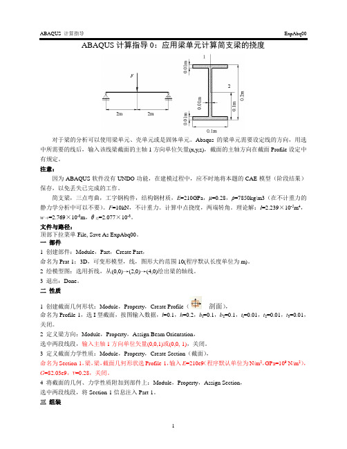
简支梁,三点弯曲,工字钢构件,结构钢材质,E=210GPa,μ=0.28,ρ=7850kg/m3(在不计重力的静力学分析中可以不要)。
F=10kN,不计重力。
计算中点挠度,两端转角。
理论解:I=2.239×10⁻⁵m4,w中=2.769×10⁻³m,θ边=2.077×10⁻³。
文件与路径:顶部下拉菜单File, Save As ExpAbq00。
一部件1 创建部件:Module,Part,Create Part,命名为Prat-1;3D,可变形模型,线,图形大约范围10(程序默认长度单位为m)。
2 绘模型图:选用折线,从(0,0)→(2,0)→(4,0)绘出梁的轴线。
3 退出:Done。
二性质1 创建截面几何形状:Module,Property,Create Profile(剖面),命名为Profile-1,选I型截面,按图输入数据,l=0.1,h=0.2,b l=0.1,b2=0.1,t l=0.01,t2=0.01,t3=0.01,关闭。
2 定义梁方向:Module,Property,Assign Beam Orientation,选中两段线段,输入主轴1方向单位矢量(0,0,1)或(0,0,-1),关闭。
3 定义截面力学性质:Module,Property,Create Section(截面),命名为Section-1,梁,梁,截面几何形状选Profile-1,输入E=210e9(程序默认单位为N/m2,GPa=109 N/m2),G=82.03e9,ν=0.28,关闭。
ABAQUS初学者使用算例

ABAQUS初学者使用算例ABAQUS/CAE实例教程我们将通过ABAQUS/CAE完成上图的建模及分析过程。
首先我们创建几何体一、创建基本特征:1、首先运行ABAQUS/CAE,在出现的对话框内选择Create Model Database。
2、从Module列表中选择Part,进入Part 模块3、选择Part→Create来创建一个新的部件。
在提示区域会出现这样一个信息。
4、CAE弹出一个如右图的对话框。
将这个部件命名为Hinge-hole,确认Modeling Space、Type和BaseFeature的选项如右图。
5、输入200作为Approximate size的值。
点击Continue。
ABAQUS/CAE初始化草图,并显示格子。
6、在工具栏选择Create Lines: Rectangle(4 Lines),在提示栏出现如下的提示后,输入(20,20)和(-20,-20),然后点击3键鼠标的中键(或滚珠)。
7、在提示框点击OK按钮。
CAE弹出Edit Basic Extrusion对话框。
8、输入40作为Depth的数值,点击OK按钮。
二、在基本特征上加个轮缘1、在主菜单上选择Shape→Solid→Extrude。
2、选择六面体的前表面,点击左键。
3、选择如下图所示的边,点击左键。
4、如右上图那样利用图标创建三条线段。
5、在工具栏中选择Create Arc: Center and 2 Endpoints6、移动鼠标到(40,0.0),圆心,点击左键,然后将鼠标移到(40,20)再次点击鼠标左键,从已画好区域的外面将鼠标移到(40,20),这时你可以看到在这两个点之间出现一个半圆,点击左键完成这个半圆。
7、在工具栏选择Create Circle: Center and Perimeter8、将鼠标移动到(40,0.0)点击左键,然后将鼠标移动到(50,0.0)点击左键。
9、从主菜单选择Add→Dimension→Radial,为刚完成的圆标注尺寸。
ABAQUS初学者使用算例

ABAQUS/CAE实例教程我们将通过ABAQUS/CAE完成上图的建模及分析过程。
首先我们创建几何体一、创建基本特征:1、首先运行ABAQUS/CAE,在出现的对话框选择Create Model Database。
2、从Module列表中选择Part,进入Part模块3、选择Part→Create来创建一个新的部件。
在提示区域会出现这样一个信息。
4、CAE弹出一个如右图的对话框。
将这个部件命名为Hinge-hole,确认Modeling Space、Type和BaseFeature的选项如右图。
5、输入200作为Approximate size的值。
点击Continue。
ABAQUS/CAE初始化草图,并显示格子。
6、在工具栏选择Create Lines: Rectangle(4 Lines),在提示栏出现如下的提示后,输入(20,20)和(-20,-20),然后点击3键鼠标的中键(或滚珠)。
7、在提示框点击OK按钮。
CAE弹出Edit Basic Extrusion对话框。
8、输入40作为Depth的数值,点击OK按钮。
二、在基本特征上加个轮缘1、在主菜单上选择Shape→Solid→Extrude。
2、选择六面体的前表面,点击左键。
3、选择如下图所示的边,点击左键。
4、如右上图那样利用图标创建三条线段。
5、在工具栏中选择Create Arc: Center and 2 Endpoints6、移动鼠标到(40,0.0),圆心,点击左键,然后将鼠标移到(40,20)再次点击鼠标左键,从已画好区域的外面将鼠标移到(40,20),这时你可以看到在这两个点之间出现一个半圆,点击左键完成这个半圆。
7、在工具栏选择Create Circle: Center and Perimeter8、将鼠标移动到(40,0.0)点击左键,然后将鼠标移动到(50,0.0)点击左键。
9、从主菜单选择Add→Dimension→Radial,为刚完成的圆标注尺寸。
ABAQUS拓扑优化手册

设计循环 (Design cycle) : 优化分析是一种不断更新设计变量的迭代过程, 执行 Abaqus 进行模型修改、查看结果以及确定是否达到优化目的。 其中每次迭代叫做一个设计循环。 优化任务 (Optimization task) : 一次优化任务包含优化的定义, 比如设计响应、 目标、 限制条件和几何约束。 设计响应(Design responses): 优化分析的输入量称之为设计响应。设计响应可以直接 从 Abaqus 的结果输出文件.odb 中读取,比如刚度、应力、特征频率及位移等。或者 Abaqus 从结果文件中计算得到模型的设计响应,例如质心、重量、相对位移等。 一个设计响应与模型紧密相关,然而,设计响应必须是一个标量,例如区域内的最大应 力或者模型体积。另外,设计响应也与特定的分析步和载荷状况有关。 目标函数(Objective functions): 目标函数决定了优化的目标。一个目标函数是从设计 响应中提取的一个标量, 如最大位移和最大应力。 一个目标函数可以用一个包含多个设计响 应的公式来表示。如果设定目标函数为最小化或者最大化设计响应,Abaqus 拓扑优化模块 则将每个设计响应值代入目标函数进行计算。另外,如果有多个目标函数,可以用权重因子 定义每个目标函数的影响程度。 约束(Constraints): 约束亦是从设计响应中提取的一个标量值。然而,一个约束不能 由设计响应的组合来表达。约束限定了设计响应 ,比如可以指定体积必须降低 45%或者某 个区域的位移不能超过 1mm。也可以指定跟优化无关的加工约束或者几何约束,比如,一 个零件必须保证能够浇铸或者冲压,又比如轴承面的直径不能改变。 停止条件(Stop conditions): 全局停止条件决定了优化的最大迭代次数。 局部停止条 件在局部最大/最小达成之后指定优化应该停止。 13.1.1.2 Abaqus/CAE 结构优化步骤
ABAQUS例题

对于梁的分析可以使用梁单元、壳单元或是固体单元。
Abaqus的梁单元需要设定线的方向,用选中所需要的线后,输入该线梁截面的主轴1方向单位矢量(x,y,z),截面的主轴方向在截面Profile设定中有规定。
注意:因为ABAQUS软件没有UNDO功能,在建模过程中,应不时地将本题的CAE模型(阶段结果)保存,以免丢失已完成的工作。
简支梁,三点弯曲,工字钢构件,结构钢材质,E=210GPa,μ=0.28,ρ=7850kg/m3(在不计重力的静力学分析中可以不要)。
F=10kN,不计重力。
计算中点挠度,两端转角。
理论解:I=2.239×10⁻⁵m4,w中=2.769×10⁻³m,θ边=2.077×10⁻³。
文件与路径:顶部下拉菜单File, Save As ExpAbq00。
一部件1 创建部件:Module,Part,Create Part,命名为Prat-1;3D,可变形模型,线,图形大约范围10(程序默认长度单位为m)。
2 绘模型图:选用折线,从(0,0)→(2,0)→(4,0)绘出梁的轴线。
3 退出:Done。
二性质1 创建截面几何形状:Module,Property,Create Profile,命名为Profile-1,选I型截面,按图输入数据,l=0.1,h=0.2,b l=0.1,b2=0.1,t l=0.01,t2=0.01,t3=0.01,关闭。
2 定义梁方向:Module,Property,Assign Beam Orientation,选中两段线段,输入主轴1方向单位矢量(0,0,1)或(0,0,-1),关闭。
3 定义截面力学性质:Module,Property,Create Section,命名为Section-1,梁,梁,截面几何形状选Profile-1,输入E=210e9(程序默认单位为N/m2,GPa=109 N/m2),G=82.03e9,ν=0.28,关闭。
- 1、下载文档前请自行甄别文档内容的完整性,平台不提供额外的编辑、内容补充、找答案等附加服务。
- 2、"仅部分预览"的文档,不可在线预览部分如存在完整性等问题,可反馈申请退款(可完整预览的文档不适用该条件!)。
- 3、如文档侵犯您的权益,请联系客服反馈,我们会尽快为您处理(人工客服工作时间:9:00-18:30)。
1) 应变能(结构刚度的度量值) 2) 特征频率 3) 内力和支反力 4) 重量和体积 5) 重心 6) 惯性矩。 可以应用其他相同约束变量到拓扑优化分析中。另外,拓扑优化同样可以考虑标准产品 制造过程。例如铸造和冲压。可以冻结指定区域、应用数量尺寸、对称性及耦合约束。拓扑 优化的例子在 ABAQUS Example Problems Manual 的 Section11.1.1 中。(本文的算例就是来自 于此)
ABAQUS 中 ATOM 模 块的拓扑优化功能
By 姜琛(BravoWa) HNU
QQ:490135416
ABAQUS 中 ATOM 模块的拓扑优化功能
从 Abaqus6.11 开始,ABAQUS/CAE 新增加了拓扑优化模块,简称 ATOM(Abaqus Topology Optimization Module),这标志着 Abaqus 开始从分析向设计进军。虽然 ABA 非线 性能力十分强大,CAE 的操作也比较人性化,但由于拓扑优化的需要,而转而采用 ANSYS 和 Hyperworks/Optistruct。ATOM 采用了专业拓扑优化软件 TOSCA 的核心,在 ABA 没有拓 扑优化模块的时候,该软件已经能通过像 FE-SAFE 那样,调用 odb 文件进行拓扑优化,但 是显然不如 ANSYS 等模块化的集成度高和操作便捷。如果将 ABA 强大非线性分析能力和 越来越完善的 ATOM 结合起来,非线性问题的拓扑优化难题应该可以得到很好的解决。
1.建立约束 couplingn, Name: Constraint-1;。如下图左选择 inp 中设置好的 set。 2.建立约束 couplingn, Name: Constraint-2;。如下图右选择 inp 中设置好的 set。
六 载荷 1 施加位移边界条件: inp 中已经施加,无需自己设定。 2 创建载荷:Name: Load-1,Step-1; Type: Concentrated force; Region: Set-CONTROLPT; Uniform, CF1=70000, CF2=-70000, CF3=0; 关闭 七 网格 inp 就是网格,略过。 八 ATOM(Module: Optimization)
设计变量(Design variables):设计变量即优化设计中需要改变的参数。拓BAQUS/CAE 优化分析模块在其优化迭代过程中改变单 元密度并将其耦合到刚度矩阵之中。实际上,拓扑优化将模型中单元移除的方法是将单元的 质量和刚度充分变小从而使其不再参与整体结构响应。对于形状优化而言,设计变量是指设 计区域内表面节点位移。优化时,ABAQUS 或者将节点位置向外移动或者向内移动,抑或 不移动。在此过程中,约束会影响表面节点移动的多少及其方向。优化仅仅直接修改边缘处 的节点,而边缘内侧的节点位移通过边缘处节点插值得到。
二 性质 1 创建材料: 将材料命名,Name: Elasti_Material;弹性,E=210000Mpa,ν=0.3;关闭。 2 创建截面: Name: Solid_Section,Solid 实体,各向同性,选上材料名 Elasti_Material,关闭。
3 将截面的性质附加到部件上: 选中 Part: Part-1,将 Section: Solid_Section 赋给 Part- Part-1。 三 组装 创建计算实体,以 Part: Part-1,用 Independent 方式生成实体。 四 分析步 分析步在 inp 文件中已经建立,命名为 Step-1,Static,Linear perturbation,静态,线性摄动步, 几何非线性 OFF。 五 接触
1.创建优化任务(Optimization Task)。从 ATOM 开始,多加入一些图; Creat:Name: controlArmTopologyOptimization; Type: Topology optimization; Continue。 然后弹出选择框,选择 Set-Design Element。 在 新 弹 出 的 ( Optimization Task Manager ) 中 , 选 择 Advanced – algorithm: Stiffness_Optimization. 关闭。
3) 弹性、塑性、全应变和应变能密度 形状优化只能应用体积约束,另外,可以使用一定数量的制造几何限制条件使提出的设计能 够继续铸造或者冲压过程。也可以冻结某特定区域、应用数量尺寸、对称性及耦合限制等。
ATOM 拓扑优化算例
本算例直接采用 ABAQUS Example Problems Manual 的 Section11.1.1 中的例子,相应的 inp 和 py 文件可在 x(x 为 ABAQUS 的安装盘):\simulia\Abaqus\6.11-1\samples\job_archive\ samples.zip 中找到,分别为 control_arm.inp 和 control_arm_topology_optimization.py。当然这 样直接使用脚本,对我们熟悉 ATOM 的操作不是很有帮助,将 py 文件逆向分析一下找到对 应的 CAE 操作。
约束(Constraints): 约束亦是从设计变量中萃取的一定范围的数值。然而,一个约束 不能由设计响应集合而来。约束限定了设计响应 ,比如可以指定体积必须降低 45%或者某 个区域的位移不能超过 1mm。约束也可以指定制造跟优化无关的制造或者几何约束,比如 轴承面的直径不能改变。
停止条件(Stop conditions): 全局停止条件决定了优化的最大迭代次数。 局部停止条 件在局部最大/最小达成之后指定优化应该停止。
2. 术语(Terminology)
设计区域(Design area): 设计区域即模型需要优化的区域。这个区域可以是整个模型, 也可以是模型的一部分或者数部分。一定的边界条件、载荷及人为约束下,拓扑优化通过增 加/删除区域中单元的材料达到最优化设计,而形状优化通过移动区域内节点来达到优化的 目的。
ATOM 中拓扑优化技术概述
1. 结构优化:概述
ABAQUS 结构优化是一个帮助用户精细化设计的迭代模块。结构优化设计能够使得结 构组件轻量化,并满足刚度和耐久性要求。ABAQUS 提供了两种优化方法——拓扑优化和 形状优化。拓扑优化(Topology optimization)通过分析过程中不断修改最初模型中指定优 化区域的单元材料性质,有效地从分析的模型中移走/增加单元而获得最优的设计目标。形 状优化(Shape optimization)则是在分析中对指定的优化区域不断移动表面节点从而达到减 小局部应力集中的优化目标。拓扑优化和形状优化均遵从一系列优化目标和约束。
3. ABAQUS/CAE 结构优化步骤
下面的步骤需要合并到 ABAQUS/CAE 模型结构优化设计中: 1) 创建需要优化的 ABAQUS 模型。 2) 创建一个优化任务。 3) 创建设计响应。 4) 利用设计响应创建目标函数和约束。 5) 创建优化进程,提交分析。
基于优化任务的定义及优化程序,ABAQUS/CAE 拓扑优化模块进行迭代运算: 1) 准备设计变量(单元密度或者表面节点位置)。 2) 更新 ABAQUS 有限元模型。 3) 执行 ABAQUS/Standard 分析。
本文目的即熟悉 ATOM 的 CAE 中的操作。首先将 ABAQUS ANALYSIS USER MANUAL 的 Topology Optimization 章节的概论部分翻译成中文,权当本文的概述(取自 SIMWE 的 Songyer 的翻译)。然后将官方提供的算例,做成 Step-by-step 以便操作。也算对本人近几天 对 ATOM 学习的总结。
设计响应(Design responses): 优化分析的输入量称之为设计响应。设计响应可以直接 从 ABAQUS 的结果输出文件.odb 中读取,比如刚度、应力、特征频率及位移等。或者 ABAQUS 从结果文件中计算得到模型的设计响应,例如质心、重量、相对位移等。一个设计响应与模 型紧密相关,然而,设计响应存在一定的范围,例如区域内的最大应力或者模型体积。另外, 设计响应也与特点的分析步和载荷状况有关。
2. 创建设计响应(Design response) 设计响应 1(Design Response 1)
Create Design Response – Name: strainEnergy; Type: Single-term; Continue. Edit Design Response – Region: Whole Model; Variable: Strain Energy; Operator: Sum of values. OK。 设计响应 2(Design Response 2) Create Design Response – Name: volume; Type: Single-term; Continue. Edit Design Response – Region: Whole Model; Variable: Volume; Operator: Sum of values. OK。
6. 形状优化
形状优化采用了跟基于刚度的拓扑优化算法类似的算法。形状优化一般是对表面节点进 行较小的调整以减小局部应力集中。形状优化用于产品外形需要微调的情况。
形状优化试图重置既定区域的表面节点位置直到此区域的应力成为常数(应力均匀)。 下图是连杆形状优化以减小局部应力集中的例子: