hypermesh梁壳单元混合建模实例(1)
2024版Hypermesh基础教程[1]
![2024版Hypermesh基础教程[1]](https://img.taocdn.com/s3/m/210c7d6a492fb4daa58da0116c175f0e7cd119f1.png)
06
前后处理技术
Chapter
2024/1/30
23
结果查看与评估
2024/1/30
查看分析结果
在Hypermesh中,用户可以通过后处理模块查看分析结果,包 括变形、应力、应变等云图,以及动画演示等。
结果评估
通过对分析结果的评估,可以判断设计是否满足要求,以及是否 需要进行优化。
结果对比
用户可以将不同设计方案的分析结果进行对比,以便更好地评估 设计的优劣。
尺寸优化流程
建立模型、定义设计变量、设置 约束条件、选择优化算法、进行 尺寸优化计算、后处理与优化结 果评估。
2024/1/30
尺寸优化应用
尺寸优化广泛应用于各种工程领 域,如建筑结构中梁、柱截面尺 寸的优化,汽车零部件尺寸的优 化等。通过尺寸优化,可以在满 足性能要求的同时,降低制造成 本和材料消耗。
随机振动分析
了解随机振动分析的基本概念和方法, 如功率谱密度、响应谱等。
05
04
瞬态动力学分析
学习瞬态动力学分析的方法和步骤, 如时域响应、频域响应等。
2024/1/30
18
05
优化设计技术
Chapter
2024/1/30
19
拓扑优化
1 2 3
拓扑优化概念 拓扑优化是一种在给定设计空间内寻找最优材料 分布的方法,旨在实现特定性能目标下的结构轻 量化。
Hypermesh基础教程
2024/1/30
1
目录
2024/1/30
• 软件介绍与安装 • 网格划分技术 • 材料属性与边界条件设置 • 结构分析基础 • 优化设计技术 • 前后处理技术
2
01
软件介绍与安装
HyperMesh+Nastran 部分资料(部分单元的创建)
rbe3单元 释放掉转 动自由度
部件1
部件2 rbe3单元 自 由度全依附 梁单元
图1-9 销轴的仿真模型的建立
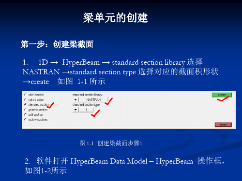
图 1-2 创建梁截面步骤2 在1处可以命名该梁截面集合,在2处可以命名该集合内部具体的梁截面。 (鼠标左键单击即可命名)。在右边的视图窗口内有数字的地方可以单 击更改其尺寸。注意横截面的坐标轴Y、Z,以后的操作中会用到。
第二步:创建梁单元属性
图 1-3 创建梁单元属性对话框
单击梁属性创建图标 ,打开创建梁属性对 话框,如图1-3所示,在prop name 里输入名字,设置color, type= 选择1D,card image=选择PBEAM,material= 选择事先 创建好的材料,beamsection= 选择事先创建好的梁的横截面。
图 1-7 设置弹簧单元的属性 在K1中设置弹簧单元的刚度,其他的系数具体所指可查阅 相关帮助、文献。 第二步:创建合适的位移坐标系
例如,用弹簧单元模拟油缸,因为油缸的轴向和 全局坐标系不平行,所以需要创建一个合适的位移坐 标系,使其中一个轴与油缸轴向重合。具体操作步骤 请见前述。
第三步:创建弹簧单元 1D → Springs → 进入到弹簧单元创建界面,如图1-8所示。
方法二:一次创建多个梁单元
具体步骤:1D → line mesh,打开创建对话框如图1-5所示:
图 1-5 创建多个梁单元
单击左上倒三角确定根据nodes还是lines来创建梁单元,element config 选择bar2, element size 设置单元的尺寸大小,其他设置和第一 种方法类似。
梁单元的创建
第一步:创建梁截面 1. 1D → HyperBeam → standard section library 选择 NASTRAN →standard section type 选择对应的截面积形状 →create 如图 1-1 所示
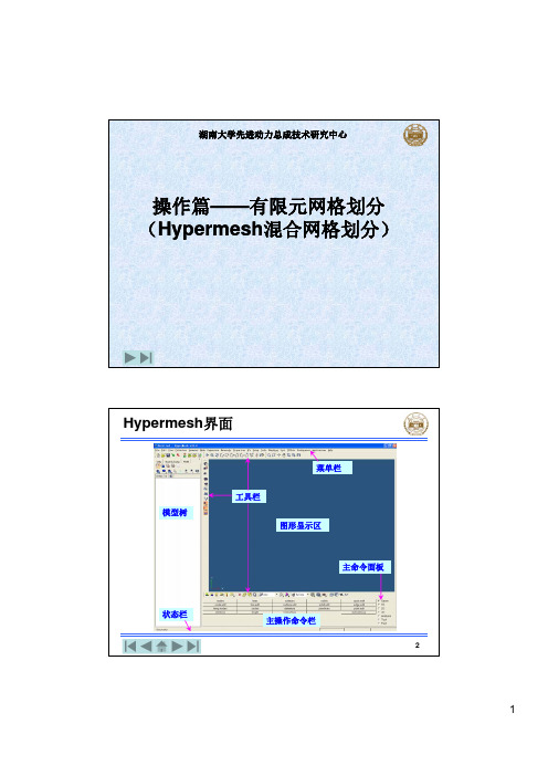
Hypermesh系列之——混合网格划分
23
法兰端网格划分
几何清理
三角形面网 格生成
打开轴颈法兰端 face网格,进行 节点重合处理。
网格质量检 生成体网
查
格
24
12
基本完成曲轴实体网格划分
25创建rbe2源自主轴颈创建5层rbe2,曲柄销创建1层。
26
13
15
曲拐二维网格划分
1、几何清理:抑制一些小边,在自动划分网格时方便生成高质量的三角形网格。
16
8
F12自动划分三角形网格
采用automesh(F12)自动划分三角形网格
17
Find face取出轴颈表面网格
保留曲拐接触面的网格
18
9
F3缝合曲拐和轴颈接触面的网格
19
F3缝合曲拐和轴颈接触面的网格
7
中心圆网格
镜像
¾.1/4中心圆二维网格必须要与外部三维网格边界节点重合(这里中心 圆最好取主轴颈的1/2)。 ¾.对1/4中心圆网格进行镜像得中心圆网格。 ¾.对中心圆二维网格进行拉伸生成三维中心网格。
8
4
完成主轴颈网格
¾.将第一主轴颈的二维网格进行复制移动到第二和第五主轴颈。因为曲 轴的第一主轴颈与后面的主轴颈不同。 ¾.对复制移动过去的二维进行旋转或拉伸生成三维。
3
4
2
Ⅰ.曲面集合分类
对曲面进行分类方便曲面分块划分网格,再把分 块的面网格进行节点重合。
5
Ⅱ.绘制二维网格
旋转
拉伸 中心圆半径一般取曲轴前段圆半径的2/3
6
3
基本要求
主轴颈横向网格数须为偶数,因为需产生主 轴颈的中心平面,最好为4层5排节点 。
hypermesh简易实用教程.
F 合适窗口大小 D display窗口H help文件F2 delete panelF12 auto mesh panel F10 elem check panel F5 mask panel F6 element edit panel Ctrl+鼠标左键旋转Ctrl+鼠标滑轮滑动缩放Ctrl+鼠标滑轮画线缩放画线部分Ctrl+鼠标右键平移F11 quick edit panel Ctrl+F2 取图片保存到F9 line edit panel R rotation 窗口F4 distance panel 可以寻找圆心W windows窗口G Global panel O Option panelShfit+F1……新窗口Shfit+F11 operation窗口Shfit+ctrl 可以透视观察Shfit+F12 smooth 对网格平顺化Shifit+F3 检查自由边,合并结点鼠标中键确认按纽Shot cut一 hypermesh网格划分⑴单元体的划分1.1 梁单元该怎么划分?Replace可以进行单元结点合并,对于一些无法抽取中面的几何体,可以采用surface offset 得到近似的中面线条抽中线:Geom中的lines下选择offset,依次点lines点要选线段,依次选中两条线,然后Creat.建立梁单元:1进入hypermesh-1D-HyperBeam,选择standard seaction。
在standard section library 下选HYPER BEAM在standard section type下选择solid circle(或者选择其它你需要的梁截面。
然后create。
在弹出的界面上,选择你要修改的参数,然后关掉并保存。
然后return.2 新建property,然后create(或者选择要更新的prop),名称为beam,在card image 中选择PBAR,然后选择material,然后create.再return.3 将你需要划分的component设为Make Current,在1D-line mesh,选择要mesh的lines,选择element size,选择为segment is whole line,在element config:中选择bar2,property选择beam(上步所建的property.然后选择mesh。
hypermesh运用实例(1)

运用HyperMesh软件对拉杆进行有限元分析问题的描述拉杆结构如图1-1所示,其中各个参数为:D1=5mm、D2=15mm,长度L0=50mm、L1=60mm、L2=110mm,圆角半径R=mm,拉力P=4500N。
求载荷下的应力和变形。
图1-1 拉杆结构图有限元分析单元单元采用三维实体单元。
边界条件为在拉杆的纵向对称中心平面上施加轴向对称约束。
模型创建过程CAD模型的创建拉杆的CAD模型使用ProE软件进行创建,如图1-2所示,将其输出为IGES格式文件即可。
图1-2 拉杆三维模型CAE模型的创建CAE模型的创建工程为:将三维CAD创建的模型保存为文件。
(1)启动HyperWorks中的hypermesh:选择optistuct模版,进入hypermesh 程序窗口。
主界面如图1-3所示。
(2)程序运行后,在下拉菜单“File”的下拉菜单中选择“Import”,在标签区选择导入类型为“Import Goemetry”,同时在标签区点击“select files”对应的图形按钮,选择“”文件,点击“import”按钮,将几何模型导入进来,导入及导入后的界面如图1-4所示。
图1-3 hypermesh程序主页面图1-4 导入的几何模型(4)几何模型的编辑。
根据模型的特点,在划分网格时可取1/8,然后进行镜像操作,画出全部网格。
因此,首先对其进行几何切分。
1)曲面形体实体化。
点击页面菜单“Geom”,在对应面板处点击“Solid”按钮,选择“surfs”,点击“all”则所有表面被选择,点击“creat”,然后点击“return”,如图1-5~图1-7所示。
图1-5 Geom页面菜单及其对应的面板图1-6 solids按钮命令对应的弹出子面板图1-7 实体化操作界面2)临时节点的创建。
点击页面菜单“Geom”,在对应面板中点击“nodes”按钮,在弹出的子面板中选择“on line”,选择如图1-8所示的五根线,点击“creat”,然后return,这样就创建了临时节点。
(完整word版)hypermesh教程
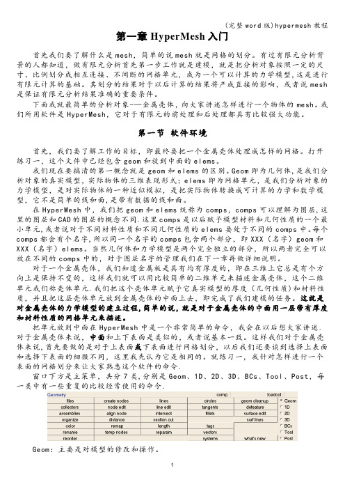
第一章 HyperMesh入门首先我们要了解什么是mesh,简单的说mesh就是网格的划分。
有过有限元分析背景的人都知道,做有限元分析首先第一步工作就是建模,就是把分析对象按照一定的尺寸、比例划分成相互连接、不间断的网格单元,成为一个可以计算的力学模型,这是进行有限元计算的基础。
其划分的结果对于以后计算的结果将产成直接的影响,或者说mesh 是保证有限元分析结果准确的重要条件。
下面我就最简单的分析对象-—金属壳体,向大家讲述怎样进行一个物体的mesh。
我们所用软件是HyperMesh,它对于有限元的前处理和后处理都具有比较强大功能。
第一节软件环境首先,我们要了解工作的目标,即最终要把一个金属壳体处理成怎样的网格。
打开练习一,这个文件中已经包含geom和放到中面的elems。
我们现在要搞清的第一概念就是geom和elems的区别。
Geom即为几何体,是我们分析对象的真实模型,实际物体的三维表现形式;elems即为网格单元,是我们分析对象的力学模型,是对实际物体的一种近似模拟,是把实际物体转换成可计算的力学和数学模型,它不是简单的线和面,是带有数据的线和面。
在HyperMesh中,我们把geom和elems统称为comps,comps可以理解为图层,这里的图层和CAD的图层的概念不同.这里comps是以后赋予模型材料和几何性质的一个最小单元,或者说对于不同材料性质和不同几何性质的elems要处于不同的comps中。
每个comps都会有个名字,所以同一个名字的comps包含两个部分,即XXX(名字)geom和XXX(名字)elems。
当然几何体和力学模型是两个完全独立的部分,所以两者完全可以放在不同的comps中的,对于图层名字的管理我们在下一章再做详细说明。
对于一个金属壳体,我们知道金属板是具有均有厚度的,即在三维上它总是有个方向上是保持不变的,这样我们就可以用比较简单的二维单元来描述金属壳体,这个二维单元我们称壳体单元.我们把这个壳体单元赋予它真实模型的厚度(几何性质)和材料性质,并且把这层壳体单元放到金属壳体的中面上去,即完成了我们建模的任务。
悬架整车性能Hypermesh有限元分析仿真试验指导书1

悬架整车性能Hypermesh有限元分析仿真试验指导书吉林大学汽车实验室编写:李静2013年10月一、实验目的(1)掌握应用有限元仿真方法分析悬架零部件的方法。
(2)了解有限元的基本思想,通过转向节强度分析实验,掌握有限元分析基本步骤。
(3)熟悉HyperMesh软件的面板,掌握HyperMesh10.0菜单布局结构,学习使用各类菜单操作。
二、实验用仪器设备及软件HyperMesh10.0能完成Hypermesh建模及计算的笔记本电脑或台式机。
三、操作步骤1.打开hypermesh,在User Profiles 窗口选择Nastran选项图1 选择求解器2.导入模型,如图2所示,三中方式任选其一:a.File >Openb.File >Importc.单击工具栏上的Import按钮单击主菜单栏上方工具栏的按钮,使模型以带表面和边框的形式显示(图3):图2 导入CAD模型图3 改变显示方式3.删除实体单击快捷键F2(删除),出现如图4所示面板,单击左上角的倒三角符号,在出现的面板图4 删除面板中选择solids, 若当前面板没有solids选项,则单击左右换页键如图5所示:图5 选择实体接下来左键单击黄色的solids选框,出现如图6所示面板,选择all或者displayed,这时整个实体模型被选中,单击主面板右上角delete entity按钮,删除实体。
图6 选中全部实体4.几何清理单击快捷键F11(快速几何编辑),出现如图7所示快速编辑面板,使用相关功能对转向节进行快速清理编辑,如添加、删除点,合并边,压缩边等,编辑完成后点击return。
图7快速几何编辑面板清除倒角选择Geom页面菜单,在Geom面板上选择defeature,出现如图8所示面板,选择surf fillets,将min radius改为0.1,max radius改为3,单击find,出现如图9所示面板,图8 defeature面板单击surfs选框,确保其出于选中状态(高亮),然后再单击转向节上需要去除的倒角面,再点击remove如图10所示图9 倒角清除面板消除前消除后图10 消除倒角自动清理在页面菜单栏,单击Geom,进入Geom面板,单击autocleanup,如图11所示图10 选择autocleanup在autocleanup面板(如图12),单击surfs选框,在他不出的面板中选择all,单击Topology cleanup parameters下方切换按钮,切换成use current parameters,单击edit parameters,出现parameters File Editor 面板,将Target element size设置为3(如图13),单击OK返回autocleanup面板图12 autocleanup面板图13 parameters File Editor单击Elements quality criteria下方切换按钮,切换成use current criteria,单击edit criteria(如图12),出现Criteria File Editor面板,将Target element size设置为3,Min Size设置为1, Max Size 设置为6(如图14), 单击OK返回autocleanup面板,单击右上角autocleanup进行自动清理。
hyperworks模态分析实例教程

Normal Modes Analysis of a Splash Shield - RD-1020In this tutorial, an existing finite element model of an automotive splash shield will be used to demonstrate how to set up and perform a normal modes analysis. HyperMesh post-processing tools are used to determine mode shapes of the model.The following exercises are included:•Retrieving the RADIOSS input file•Setting up the model in HyperMesh•Applying Loads and Boundary Conditions to the Model•Submitting the job•Viewing the resultsStep 1: Launch HyperMesh and set the RADIOSS (Bulk Data) User Profileunch HyperMesh.A User Profiles… Graphic User Interface (GUI) will appear. If it does not appear, go to Preferences►User Profiles … from the menu on the top.2.Select RADIOSS in the User Profile dialog.3.From the extended list, select Bulk Data.4.Click OK.This loads the User Profile. It includes the appropriate template, macro menu, and import reader, paring down the functionality of HyperMesh to what is relevant for generating models in Bulk Data Format for RADIOSS and OptiStruct.Step 2: Import a Finite Element Model File in HyperMesh1.From the File pull-down menu on the toolbar, select Import….An Import… tab is added to your tab menu.2.Click to import an FE model.3.For the File type:, select RADIOSS (Bulk Data).4.Select the Files icon button.A Select RADIOSS (Bulk Data) file browser will pop up.5.Browse for sshield.fem file located in the HyperWorks installation directory under<install_directory>/tutorials/hwsolvers/radioss/ and select the file.6.Click Open►Import.7.Click Close to close the Import tab menu.Step 3: Review Rigid ElementsNotice there are two rigid "spiders" in the model. They are placed at locations where the shield is bolted down. This is a simplified representation of the interaction between the bolts and the shield. It is assumed that the bolts are significantly more rigid in comparison to the shield.The dependent nodes of the rigid elements have all six degrees of freedom constrained. Therefore, each "spider" connects nodes of the shell mesh together in such a way that they do not move with respect to one another.The following steps show how to review the properties of the rigid elements.1.From the 1D page, select the rigids.2.Click review.3.Select one of the rigid elements in the graphics region.In the graphics window, HyperMesh displays the IDs of the rigid element and the two end nodes and indicates the independent node with an 'I' and the dependent node with a 'D'. HyperMesh also indicates the constrained degrees of freedom for the selected element, through the dof checkboxes in the rigids panel. All rigid elements in this model should have all dofs constrained.4.Click return to go to the main menu.Step 4: Setting up the Material and Geometric PropertiesThe imported model has three component collectors with no materials. A material collector needs to be created and assigned to the shell component collectors. The rigid elements do not need to be assigned a material. Shell thickness values also need to be corrected.1.Select the Material Collectors toolbar button .2.Select the create subpanel using the radio buttons on the left-hand side of the panel.3.Click mat name = and enter steel.4.Select the desired color for the material steel by clicking on .5.Click card image = and select MAT1 from the pop-up menu.6.Click create/edit.The MAT1 card image pops up.7.For E, enter the value 2.0E5.8.For NU, enter the value 0.3.9.For RHO, enter the value 7.85E-9.If a quantity in brackets does not have a value below it, it is off. To change this, click the quantity in brackets and an entry field will appear below it. Click in the entry field, and a value can be entered.10.Click return.A new material, steel, has now been created. The material uses RADIOSS linear isotropic materialmodel, MAT1. This material has a Young's Modulus of 2E+05, a Poisson's Ratio of 0.3 and a material density of 7.85E-09. A material density is required for the normal modes solution sequence.At any time the card image for this collector can be modified using Card Editor.11.Click return to exit the Material Create panel.12.Select the Card Editor toolbar button .13.Click the down arrow on the right of the entity shown in the yellow box, select props from the extendedentity list.14.Click the yellow props button and then check the box next to design and nondesign.15.Click select.16.Make sure card image=is set to PSHELL.17.Click edit.The PSHELL card image for the design component collector pops up.18.Replace 0.300 in the T field with 0.25.19.Click return to save the changes to the card image.20.Click return to go to the main menu.Applying Loads and Boundary Conditions to the Model (Steps 5 - 7)The model is to be constrained using SPCs at the bolt locations, as shown in the following figure. The constraints will be organized into the load collector 'constraints'.To perform a normal modes analysis, a real eigenvalue extraction (EIGRL) card needs to be referenced in the subcase. The real eigenvalue extraction card is defined in HyperMesh as a load collector with an EIGRL card image. This load collector should not contain any other loads.Step 5: Create EIGRL card (to request the number of modes)If a quantity in brackets does not have a value below it, it is off. To change this, click on the quantity in brackets and an entry field will appear below it. Click on the entry field, and a value can be entered.Step 6: Create Constraints at Bolt LocationsSelecting nodes for constraining the bolt locations 1.Click the Load Collectors toolbar button .2.Select the create subpanel, using the radio buttons on the left-hand side of the panel.3.Click loadcol name = and enter EIGRL .4.Click card image= and select EIGRL from the pop-up menu.5.Click create/edit .6.For V2, enter the value 200.000.7.For ND , enter the value 6.8.Click return to save changes to the card image.1.Click loadcol name = and enter constraints .2.Click the switch next to card image and select no card image .3.Click create > return .4.From Analysis page, click the constraints panel and make sure that the createsubpanel is active.5.Select the two nodes, shown in the figure above, at the center of the rigid spiders, by clicking on them in the graphics window.6.Constrain all dofs with a value of 0.0.7.Click Load Type= and select SPC .8.Click createTwo constraints are created. Constraint symbols (triangles) appear in the graphics window at theselected nodes. The number 123456 is written beside the constraint symbol, if the label constraints is checked ‘ON’, indicating that all dofs are constrained.9.Click return to go the main menu.Step 7: Create a Load Step to perform Normal Modes Analysis1.From the Analysis page, enter the loadsteps panel.2.Click name = and enter bolted.3.Click the type: switch and select normal modes from the pop-up menu.4.Check the box preceding SPC.An entry field appears to the right of SPC.5.Click on the entry field and select constraints from the list of load collectors.6.Check the box preceding METHOD(STRUCT).An entry field appears to the right of METHOD.7.Click on the entry field and select EIGRL from the list of load collectors.8.Click create.A RADIOSS subcase has been created which references the constraints in the load collector constraintsand the real eigenvalue extraction data in the load collector EIGRL.9.Click return to go to the main menu.Submitting the JobStep 8: Running Normal Modes Analysis1.From the Analysis page, enter the RADIOSS panel.2.Click save as… following the input file:field.A Save file… browser window pops up.3.Select the directory where you would like to write the file and, in File name:, entersshield_complete.fem.4.Click Save.Note that the name and location of the sshield_complete.fem file shows in the input file: field.5.Set the export options:toggle to all.6.Click the run options: switch and select analysis.7.Set the memory options: toggle to memory default.8.Click Radioss.This launches the RADIOSS job.If the job was successful, new results files can be seen in the directory where the RADIOSS model file was written. The sshield_complete.out file is a good place to look for error messages that will help to debug the input deck if any errors are present.The default files written to your directory are:sshield_complete.html HTML report of the analysis, giving a summary of the problemformulation and the analysis results.sshield_complete.out RADIOSS output file containing specific information on the file setup, the set up of your optimization problem, estimates for the amountof RAM and disk space required for the run, information for eachoptimization iteration, and compute time information. Review this fileReview the Results using HyperViewEigenvector results are output by default, from RADIOSS for a normal modes analysis. This section describes how to view the results in HyperView.Step 9: Load the Model and Result Files into the Animation WindowIn this section, you will load a HyperView .h3d file into the HyperView animation window.HyperView is launched and the sshield_complete.h3d file is loaded.Step 10: View Eigen VectorsIt is helpful to view the deformed shape of a model to determine if the boundary conditions have been defined correctly and also to check if the model is deforming as expected. In this section, use the Deformed panel to review the deformed shape for last Mode .This means that the maximum displacement will be 10 modal units and all other displacements will be proportional.Using a scale factor higher than 1.0 amplifies the deformations while a scale factor smaller than 1.0 would reduce them. In this case, we are accentuating displacements in all directions.A deformed plot of the model overlaid on the original undeformed mesh is displayed in the graphics window. for warnings and errors.sshield_complete.h3dHyper 3D binary results file. sshield_complete.stat Summary of analysis process, providing CPU information for eachstep during analysis process. 1.Click the HyperView button in the RADIOSS panel. 2.Click Close to exit the Message Log menu that appears.1.Click on the switch next to the traffic light signaland select Modal .2.Select the Deformed toolbar button.3.Leave Result type:set to Eigen Mode (v).4.Set Scale: to Model units .5.Set Type: to Uniform and enter in a scale factor of 10 for Value:.6.Click Apply .7.Under Undeformed shape:, set Show: to Wireframe .8.From the Graphics pull-down menu, select Select Load Case to activate the Load Case andSimulation Selection dialog, as shown below.Step 11: A few points to be notedIn this analysis, it was assumed that the bolts were significantly stiffer than the shield. If the bolts needed to be made of aluminum and the shield was still made of steel, would the model need to be modified, and the analysis run again?It is necessary to push the natural frequencies of the splash shield above 50 Hz. With the current model, there should be one mode that violates this constraint: Mode 1. Design specifications allow the innerdisjointed circular rib to be modified such that no significant mass is added to the part. Is there a configuration for this rib within the above stated constraints that will push the first mode above 50 Hz? See tutorial OS-2020 to optimize rib locations for this part.Go ToRADIOSS, MotionSolve, and OptiStruct Tutorials9.Select Mode 6 - F=1.496557E+02 from the list and click OK to view Mode 6.10.To animate the mode shape, click the animation mode: modal.11.To control the animation speed, use the Animation Controls accessed with the director’s chair toolbar button .12.You could also review the rest of the mode shapes.。
hypermesh实例教学

5.练习
• base_bracket.hm
6.创建和编辑线line
7.网格质量检查和编辑(面)
• cover.hm。主要检查网格的连续性、法向、 质量差的单元修改。 • SHIFT+F3 网格连续检测。两个曲面共享的 边界,应该没有曲线,如果有则说明两个 面之间的单元不连续。 • “^”,部件componet名称,如果以“^”开 头,则该部件不作为输出文件导出。 • 调整tolerance= field的值,使用preview equiv查找出网格不连续的node。 • SHIFT+F10检查单元法线方向。
Hyperworks实例
1. 几何清理(实体)
• Non-manifold :两个以上的面共用一条边。黄色。处理 措施为删除其中多余的面。 • Keep tangency :使由封闭曲线构成的面与封闭曲线相 切。 • Auto create (free edges):选择封闭曲线的1条边后,其
它边自动选择。 • F2:删除命令。快捷键。
• O:设置几何曲面连接误差,如设置: cleanup tol =0.1 • Equivalence:等效。小于 cleanup tol =0.1的曲面将会自 动封闭。 • Toggle ,其效果与Equivalence 一样。cleanup tol =0.1。 但Toggle还有另外一个作用是将绿色的轮廓线变为虚线, 则虚线不参与网格的划分。
4.提高曲面的拓扑结构
减少短边,使各个分块更加均匀。 • 通过移除硬点, point edit_replace point edit_replace • 移除内部无用的硬点interior fixed points , point edit_suppress • 重新划分曲面。F11 • F4。测量节点(NODE)或硬点(POINT)之间的距离。 • 使用Surface Edges > (Un)Suppress 或toggle去掉能引起小 网格的小边。 • SHITT+F2.删除多余的node. • 注意:对称体。如园、圆柱体,要从中心或中心面对称 剖开。
基于HyperMesh的商用车驱动桥壳有限元分析
收 稿 日 期 :2009-03-22 4054 计算机工程应用技术
本栏目责任编辑:贾薇薇
第 5 卷第 15 期 (2009 年 5 月)
极为不利,应尽量避免这种情况产生。 驱后轴载荷 12430kg,发动机最大输出 扭 矩 1550N/m,变速箱 1 档速比 12.10,后桥主减速器速比 4.38,驱动 轮轮 胎 滚 动 半 径 0.47m。 车 桥 材 料 屈 服 强 度 σs≥400MPa,抗 拉 强 度 σb=550MPa。 根据驱动桥的实际行驶工况,在轮轴处约束,板簧 处加载。 冲击载荷工况下等效应力图和变形图如图 2、图 3,侧向 力最大工况下等效应力图和变形图如图 4、图 5,其余工况应力和 位移如表 1、表 2。
冲击载荷工况下等效应力图和变形图如图3侧向力最大工况下等效应力图和变形图如图5其余工况应力和位移如表侧向力最大工况下变形图计算结果表明最大应力基本出现在轮毂内轴承里端在侧向力最大的极限工况下比较危险还有在冲击载荷工况下最大应力很接近材料的屈服强度其余工况满足材料刚度和强度要求安全系数较高
ISSN 1009-3044 CCoommppuutteerr KKnnoowwlleeddggee aanndd TTeecchhnnoollooggyy 电电脑脑知知识识与与技技术术
Vol.5,No.15, May 2009, pp.4054-4055
E-mail: kfyj@ 第 5 卷第 15ht期tp://w(w2w00.d9nz年s.n5et月.cn)
Tel:+86-551-5690963 5690964
基于 Hyper Mesh 的商用车驱动桥壳有限元分析
hypermesh梁壳单元混合建模实例

HyperMesh梁单元和壳单元的混合建模本文根据工程实例,应用有限元软件HyperMesh 11.0进行梁单元和壳单元的混合建模,并在其中详细论述,梁单元在与壳单元混合建模的过程中如何对梁单元进行偏置处理,保证梁单元与壳单元的所有节点完全耦合。
在焊接工艺中,梁单元与壳单元的使用可以大大提高整体焊接结构的抵抗变形能力,避免单独使用壳单元时强度和刚度的不足。
HyperMesh软件中提供了大量标准梁的截面,也可以通过实际应用需求单独创建梁截面。
在1D面板中点选HyperBeam选项,如图1所示。
图1 1D面板中的HyperBeam选项HyperBeam中提供了大量的梁截面,如图2所示。
图2 HyperBeam下的各种梁截面图2中红色箭头所指的是各种标准梁截面的属性,包括H型梁,L型梁,工型梁等等。
可以根据实际需求进行选择,而且可以自己独立进行尺寸编辑。
图2中的shell section可以建立独立的壳截面,solid section可以建立独立的实体截面。
在建立完成各种梁的截面属性之后,可以通过edit section进行梁截面属性的修改。
以上主要介绍了1D梁单元的使用情况,下面将根据工程实例对壳单元和梁单元的混合建模进行详细的介绍。
图3是梁单元和壳单元焊接之后的三维图,图4是图3中梁单元以1D显示的情况。
二者之间的切换功能键如图5所示。
图3 梁单元和壳单元焊接之后梁单元以3D显示图4 梁单元和壳单元焊接之后梁单元以1D显示图5 梁单元1D与3D之间的切换功能键下面介绍梁单元的具体创建方法,不再讲述壳单元的建立方法。
首先建立Beam Section,在软件左侧右键create--Beam Section,在出现的对话框窗口中对Bean进行命名。
具体的过程如图6所示。
图6 Beam的建立过程之后进入1D--HyperBeam面板,选择Standard section选择Standard Channel面板,打开面板后对各个参数进行修改,如图7所示。
hypermesh-CAE实例

车身CAE—零件受力分析
姓名:韦小刚
班级:2009-47 车辆工程
学号:S0908*******
利用CATIA建模导入Hypermesh分析1 CATIA建模
建立零部件part1、Part2。
进入开始--形状--创成式曲面设计。
选择一个平面建立草图。
然后经过拉伸成片体。
最后将模型保存为igs 格式文件。
图-1
2 打开Hypermesh,导入igs文件
图-2
3 建立材料集合器编辑材料常数
图-3 4 建立属性集合器并编辑属性
图-4 5 创建单元集合器
图-5
6 划分单元并检查单元质量
7 建立刚性连接单元
图-6
图-7
8 创建载荷、约束集合器,加载和约束
图-8
9 创建控制卡片、载荷步。
Control cards:Sol选项里选择static;param选项里选择autospc、bailout(-1)、post(-2)选项。
图-9
Loadsteps
图-10
10 定义输出选项,求解
Export
Export type:FE model
File type :optistruct
Templare:standard format
File选项里后缀名为.fem。
图-11 11 观察结果—利用hyperview Op2文件导入hyperview
位移云图:
图-12 应力云图:
图-13。
HYPERMESH实例分析课件

5、几何清理
A 导入几何模型:通过FILE_IMPORT子面板(IGES:可 导入*.igs)文件
文件地址:
D:/altair/tutorials/hm/raw_iges_data .iges
精
精
点击
改变边显示模式
精
B 模型几何的拓扑显示: 自由边:自由边只属于一个曲面,默认颜色为红色。在 一个经过几何清理的模型中,自由边通常只存在于部件的 外周或者环绕在内部孔洞的周围。 共享边:共享边被两个相邻曲面所共有,默认颜色为绿色。 压缩边:压缩边为两个相邻曲面所共有,但在划分网格时 被忽略被压缩边,不会生成节点,默认颜色为蓝色 T型连接边:表示曲面的边界被三个或三个以上的曲面所 共享,默认颜色为黄色
精
面板菜单:显示每一页面上可用的功能,可通过点击与功 能相应的按钮来实现这些功能
标签域:位于图形区域的左侧,列出一些很有用的工具, 包含多个特征页面,如UTILITY菜单,MODEL浏览器, 和SOLVER浏览器等
命令窗口:可将HYPERMESH的命令直接键入文本框执行 的方式代替使用图形用户界面功能执行命令
精
导入文件(HM/CAD/FEM) 设置模
版
几何清理
建立材料卡片
建立几何,单元集
划分单元
单元检查与优化 建立载荷集 施加
载荷 建立载荷工况 设置计算参数
输出有限元文件 求解器求解 进行
后处理
精
3、HYPERMESH8.0窗口界面
主要包括以下几个窗口界面: 下拉菜单 图形区 工具栏 标题栏 页面菜单 面板菜单 标签域 命令窗口
有限元分析分为三大步:有限元前处理,有限元求解,有 限元后处理。
abaqus模板在hypermesh中建立beam梁单元的详细步骤

1.点击下图按钮,弹出hyperbeam view界面,如第二步图
①
2.在左侧空白处右键单击,选择自己想要的截面形状,并输入截面参数
②
③
3.点击model view按钮返回,发现出现了新建的beam section
④
4.创建属性,输入prop name,type选择line section,card image选择beamsection,选择相应的material,点击beamsection出现了刚才建立的截面属性,点击它
5.点击右侧creat/edit按钮,打开卡片截面,勾选section axis,输入截面主轴(y轴)在建模环境中的恰当方向。
(观察刚刚在建立截面属性时出现的截面局部坐标y轴,在建模环境中应将其设置为和x轴或y 轴平行,因此这里输入x轴的方向,【1,0,0】)
6.返回主界面,点击line mesh按钮,进入梁单元创建界面。
Node list选择两端节点,设定element size,选择property,选择bar2,点击mesh,如果想修改单元个数就修改,之后return。
Hypermesh与Nastran模态分析详细教程
Hypermesh & Nastran 模态分析教程摘要:本文将采用一个简单外伸梁的例子来讲述Hypemesh 与Nastran 联合仿真进行模态分析的全过程。
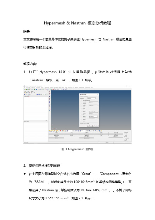
教程内容:1.打开”Hypermesh 14.0”进入操作界面,在弹出的对话框上勾选‘nastran’模块,点‘ok’,如图1.1 所示。
图1.1-hypermesh 主界面2.梁结构网格模型的创建在主界面左侧模型树空白处右击选择‘Creat’ –‘Component’,重命名为‘BEAM’,然后创建尺寸为100*10*5mm3的梁结构网格模型。
(一开始选择了Nastran后,单位制默认为N, ton, MPa, mm.)。
本例子网格尺寸大小为2.5*2.5*2.5mm3,如图2.1 所示:图2.1-梁结构网格模型3.定义网格模型材料属性●在主界面左侧模型树空白处右击选择‘Creat’–‘Material’,如图3.1所示:图3.1-材料创建●在模型树内Material下将出现新建的材料‘Material 1’,将其重命名为’BEAM’。
点击‘BEAM’,将会出现材料参数设置对话框。
本例子采用铁作为梁结构材料,对于模态分析,我们只需要设定材料弹性模量,泊松比,密度即可。
故在参数设置对话框内填入一下数据:完整的材料参数设置如图3.2所示:图3.2-Material材料参数设置同理,按同样方式在主界面左侧模型树空白处右击选择‘Creat’ –‘Pro perty’,模型树上Property下将出现新建的‘Property1’,同样将其重命名为‘BEAM’,点击Property下的‘BEAM’出现如图所示属性参数设置对话框。
由于本例子使用的单元为三维体单元,因此点击对话框的‘card image’选择‘PSOLID’,点击对话框内的Material选项,选择上一步我们设置好的材料‘BEAM’,完整的设置如图3.3所示:图3.3-Property属性设置最后,点击之前创建的在Component 下的‘BEAM’模型,将出现以下对话框(图3.4),把Property 和Material 都选上对应的‘BEAM’,完成网格模型材料属性的定义。
- 1、下载文档前请自行甄别文档内容的完整性,平台不提供额外的编辑、内容补充、找答案等附加服务。
- 2、"仅部分预览"的文档,不可在线预览部分如存在完整性等问题,可反馈申请退款(可完整预览的文档不适用该条件!)。
- 3、如文档侵犯您的权益,请联系客服反馈,我们会尽快为您处理(人工客服工作时间:9:00-18:30)。
HyperMesh梁单元和壳单元的混合建模本文根据工程实例,应用有限元软件HyperMesh 进行梁单元和壳单元的混合建模,并在其中详细论述,梁单元在与壳单元混合建模的过程中如何对梁单元进行偏置处理,保证梁单元与壳单元的所有节点完全耦合。
在焊接工艺中,梁单元与壳单元的使用可以大大提高整体焊接结构的抵抗变形能力,避免单独使用壳单元时强度和刚度的不足。
HyperMesh软件中提供了大量标准梁的截面,也可以通过实际应用需求单独创建梁截面。
在1D面板中点选HyperBeam选项,如图1所示。
图1 1D面板中的HyperBeam选项
HyperBeam中提供了大量的梁截面,如图2所示。
图2 HyperBeam下的各种梁截面
图2中红色箭头所指的是各种标准梁截面的属性,包括H型梁,L 型梁,工型梁等等。
可以根据实际需求进行选择,而且可以自己独立进行尺寸编辑。
图2中的shell section可以建立独立的壳截面,solid section可以建立独立的实体截面。
在建立完成各种梁的截面属性之后,可以通过edit section 进行梁截面属性的修改。
以上主要介绍了1D梁单元的使用情况,下面将根据工程实例对壳单元和梁单元的混合建模进行详细的介绍。
图3是梁单元和壳单元焊接之后的三维图,图4是图3中梁单元以1D显示的情况。
二者之间的切换功能键如图5所示。
图3 梁单元和壳单元焊接之后梁单元以3D显示
图4 梁单元和壳单元焊接之后梁单元以1D显示
图5 梁单元1D与3D之间的切换功能键
下面介绍梁单元的具体创建方法,不再讲述壳单元的建立方法。
首先建立Beam Section,在软件左侧右键create--Beam Section,在出现的对话框窗口中对Bean进行命名。
具体的过程如图6所示。
图6 Beam的建立过程
之后进入1D--HyperBeam面板,选择Standard section选择Standard Channel面板,打开面板后对各个参数进行修改,如图7所示。
左侧的红色框内的区域是进行具体尺寸的修改,修改的结果会以直观的形式显示在图形界面中,右侧的红色方框是梁界面的各个力学参数。
注意梁的方向,梁的长度方向是X轴,图形中的是梁的Y轴和Z轴。
在梁的方向的选取过程中Y轴为第一方向。
图7 梁的各个参数的修改
之后建立梁的属性,同样在软件左侧位置右键创建属性,弹出属性创建的选项卡片,在Type中选择1D,在Card image中选择PBEAM,单击确定按钮,如图8所示。
图8 梁属性的创建及其卡片的设置
以上过程都处理好之后进行具体梁与壳单元的混合建模,进入1D--line mesh卡片里面,如图9所示。
图9 1D--line Mesh卡片
进入之后会发现有很多按钮,具体的功能介绍:左上角位置是进行节点或或者线的选择,也就是说梁在节点或者线上进行创建。
左下角的auto功能键是确定梁的如何摆放,element config是选择进行梁还是杆的创建,文中我们选择bar2。
Offset是表示梁向哪个方向进行偏置,ax ay az表示梁单元的第一个端点,bx by bz表示梁单元的第二个端点。
具体如图10所示:
图10 Line Mesh具体功能图
在已经建立好的壳单元中选择一排节点,并建立一个壳单元与梁单元的混合建模,按照图5把梁单元的显示方式切换为3D,建立好的有限元模型图如图11所示:
图11 梁单元与壳单元混合模型的3D显示
由图11可以看出,虽然梁单元与壳单元进行了混合建模,但是3D 情况下二者之间仍有缝隙,为了能够和实际梁单元和壳单元焊接一样,要进行梁单元的偏置。
把梁单元的x轴进行偏置,偏置的过程要依据梁截面的属性和壳的厚度进行计算,偏置后的3D显示如图12所示:
图12 偏置后的梁与壳单元的3D显示图
以上过程中介绍了如何应用HyperMesh软件进行梁单元与壳单元的混合建模,以及梁单元面板中各个参数的如何设置及其说明,希望能够为广大工程人员提供帮助。