经济计量学练习题(全英文)
伍德里奇计量经济学英文题库
伍德里奇计量经济学英文题库The Econometrics Exam Bank of WoodridgeEconometrics is a field of study that combines economic theory, mathematics, and statistics to analyze and interpret economic data. It is a crucial tool for policymakers, researchers, and analysts who seek to understand the complex relationships between economic variables and make informed decisions. One of the pioneers in this field is Jeffrey Woodridge, whose contributions to econometrics have been widely recognized and celebrated.Woodridge's work has had a profound impact on the way we approach and analyze economic data. His expertise in panel data analysis, time series econometrics, and microeconometrics has been instrumental in shaping the field of econometrics. Woodridge's textbook "Econometric Analysis of Cross Section and Panel Data" has become a standard reference for students and researchers in the field, and his research has been published in numerous prestigious academic journals.One of the key areas of Woodridge's work is the development of econometric models and techniques that can be used to analyzecomplex economic phenomena. For example, his research on panel data analysis has provided researchers with powerful tools for studying the behavior of individuals, firms, or countries over time. By incorporating both the cross-sectional and time-series dimensions of data, panel data analysis allows for a more nuanced understandingof the factors that drive economic outcomes.Woodridge has also made significant contributions to the field of time series econometrics. His work on topics such as unit root testing, cointegration analysis, and vector autoregressive (VAR) models has helped researchers to better understand the dynamic relationships between economic variables over time. These techniques are particularly important in areas such as macroeconomics, where policymakers need to understand the long-term trends and short-term fluctuations in key economic indicators.In addition to his research, Woodridge has also been a dedicated educator, sharing his knowledge and insights with students and colleagues around the world. His textbooks and course materials have been widely adopted by universities and research institutions, and he has mentored countless graduate students and young researchers.One of the key features of Woodridge's approach to econometrics is his emphasis on practical applications and real-world relevance. Hehas always been committed to ensuring that his work has a direct impact on the lives of people and the decisions of policymakers. Whether it's analyzing the effects of government policies on economic outcomes or exploring the drivers of consumer behavior, Woodridge's work is grounded in a deep understanding of the practical challenges and concerns that shape the economic landscape.Moreover, Woodridge's contributions to econometrics have extended beyond the academic realm. He has served as a consultant and advisor to various government agencies, international organizations, and private sector firms, providing his expertise and insights to help inform decision-making and policy development.In conclusion, the econometrics exam bank of Woodridge is a testament to his enduring legacy and the profound impact of his work. Through his groundbreaking research, innovative teaching, and tireless efforts to bridge the gap between theory and practice, Woodridge has made an indelible mark on the field of econometrics. His contributions have not only advanced our understanding of economic phenomena but have also equipped generations of researchers and policymakers with the tools and insights they need to tackle the complex challenges of the modern world.。
高级计量经济学试题final_2005a

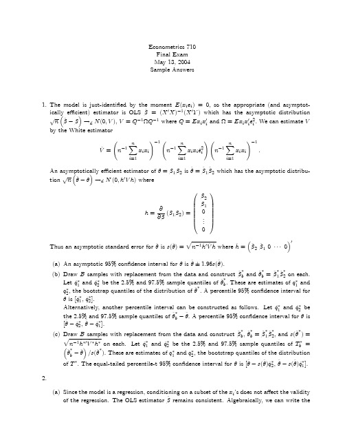
Econometrics710Final ExamSpring,2005Sample Answers1.The moment equations areEg i(µ)=0g i(µ)=µy i−µx i¶There are two moments,one parameter,so the model is overidentified.Let Ω=Eg i g0i=µE(y i−µ)2E(x i(y i−µ))E(x i(y i−µ))Ex2i¶=µσ2yσxyσxyσ2x¶where we make use of the knowledge that Ex i=0.Letg n(µ)=1nnX i=1g i(µ)=µy n−µx n¶andˆΩ=µˆσ2yˆσxyˆσxyˆσ2x¶=µ1P n i=1(y i−y n)21P n i=1(y i−y n)x i1P n i=1(y i−y n)x i1P n i=1x2i ¶The efficient GMM estimatorˆµforµminimizes J n(µ)=ng n(µ)0Ω−1g n(µ)=nˆσ2yˆσ2x−ˆσ2xy¡y n−µx n¢µˆσ2x−ˆσxy−ˆσxyˆσ2y¶µy n−µx n¶=nˆσ2yˆσ2x−ˆσ2xy¡ˆσ2x(y n−µ)2−2ˆσxy(y n−µ)x n+ˆσ2y x2n¢The minimizer isˆµ=y n−ˆσxyˆσ2xx n.(1) Side Note:Interestingly,this is the same as the intercept from the OLS estimate of the equationy i=ˆµ+ˆβx i+e i.The important point is that the efficient GMM estimator(1)is not simply the sample mean y n.The latter is a GMM estimator,but it not efficient when we add the information that Ex i=0.(Unlessσxy=0,in which case the sample mean is efficient.However,this is not assumed in the question.)2.Substituting y i =x 0i β+εi ,we obtain˜β−β=ÃnX i =1ε−2i x i x 0i!−1ÃnX i =1ε−2i x i εi !=Ã1nn X i =1ε−2i x i x 0i!−1Ã1nn X i =1ε−1i x i!By the WLLN,1n nX i =1ε−2ix i x 0i →p E ¡ε−2i x i x 0i ¢=Q,1n nX i =1ε−1ix i →p E ¡ε−1i x i ¢=δIn general,δ=0,so ˜β→p β+Q −1δ.ˆβis consistent for βi ffδ=0.If εi is symmetric about zero,and E |εi |−1<∞then E ¡ε−1i |x i ¢=0andδ=E ¡ε−1i x i ¢=E ¡x i E ¡ε−1i |x i ¢¢=0.Furthermore,note thatE ¡ε−1i x i −뛭ε−1i x i −δ¢0=E ¡ε−2i x i x 0i ¢−δδ0=Q −δδ0.Then by the CLT1√n nX i =1¡ε−1i x i −δ¢→d N (0,Q −δδ0)Thus √n ³˜β−(β+δ)´→d N (0,V )whereV =Q −1(Q −δδ0)Q −1=Q −1−Q −1δδ0Q −1.In the case where δ=0,this is√n ³˜β−β´→d N ¡0,Q−1¢Infeasible GLS has the asymptotic distribution √n ³˜βGLS −β´→d N (0,V GLS )V GLS =¡E ¡σ−2i x i x 0i¢¢−1By Jensen’s inequalityE ¡ε−2i |x i ¢≥¡E ¡ε2i |x i ¢¢−1=σ−2i .ThereforeQ=E¡ε−2i x i x0i¢=E¡x i x0i E¡ε−2i|x i¢¢≥E¡x i x0iσ−2i¢and thusV=Q−1≤E¡x i x0iσ−2i¢−1=V GLSWe can conclude that the infeasible estimator˜βis more efficient than infeasible GLS(when δ=0).This seems impossible,as we know that GLS is asymptotically efficient.The trick is that there is no feasible version of˜βwhich attains the same distribution,so the efficient gain is empirically irrelevant.3.The model is just identified,so is estimated by OLS.Write the estimates asy i=x01iˆβ1+x02iˆβ2+ˆe iLetˆV=Ã1n n X i=1x i x0i!−1Ã1n n X i=1x i x0iˆe2i!Ã1n n X i=1x i x0i!−1.The Wald statistic to test H0isW n=n³ˆβ1−ˆβ2´0³R0ˆV R´−1³ˆβ1−ˆβ2´R=µI k−I k¶To do a nonparametric bootstrap test,we sample(y∗i,x∗i)jointly from the observations.On each bootstrap sample,we construct the OLS estimatesy∗i=x∗01iˆβ∗1+x∗02iˆβ∗2+ˆe∗icovariance matrixˆV∗=Ã1n n X i=1x∗i x∗0i!−1Ã1n n X i=1x∗i x∗0iˆe∗2i!Ã1n n X i=1x∗i x∗0i!−1.and Wald statisticW∗n=n³³ˆβ∗1−ˆβ∗2´−³ˆβ1−ˆβ2´´0³R0ˆV∗R´−1³³ˆβ∗1−ˆβ∗2´−³ˆβ1−ˆβ2´´It is very important that the statistic is centered at the sample values³ˆβ1−ˆβ2´,rather than at the hypothesized value of0.The estimated bootstrap p-value is the percentage of the simulated W∗n that are largely than the sample value W n.If there are B bootstrap replications,this isp∗n=1BBX b=11(W∗n(b)≥W n).4.The GMM criterion isJ n (β)=ng n (β)0ˆΩ−1g n (β)g n (β)=1n (X 0Y −X 0Zβ)ˆΩ=1n X i =1x i x 0i ˆe 2i ˆe i =y i −z 0i ˆβLetˆβ=³Z 0X ˆΩ−1X 0Z ´−1Z 0X ˆΩ−1X 0Y denote the unconstrained GMM estimator.The Lagrangian can be written asJ n (β,λ)=12nJ n (β)−λ0R 0βwhere λ∈R q is a Lagrange multiplier.The factor 1/2n is unimportant but makes thecalculations easier.The constrained estimator (˜β,˜λ)minimizes J n (β,λ).The first order conditions are0=∂∂βJ n (˜β,˜λ)=−Z 0X ˆΩ−1X 0³Y −Z ˜β´−R ˜λ(2)0=∂J n (˜β,˜λ)=R 0˜βPremultiply (2)by ³Z 0X ˆΩ−1X 0Z ´−1to obtain³Z 0X ˆΩ−1X 0Z´−1R ˜λ=−³Z 0X ˆΩ−1X 0Z ´−1Z 0X ˆΩ−1X³Y −Z ˜β´(3)=˜β−ˆβ.Premultiplying by R 0,using R 0˜β=0,and solving,˜λ=−µR 0³Z 0X ˆΩ−1X 0Z ´−1R ¶−1R 0ˆβ.Substituting this into (3)we find˜β=ˆβ−³Z 0X ˆΩ−1X 0Z ´−1R µR 0³Z 0X ˆΩ−1X 0Z ´−1R ¶−1R 0ˆβ5.LetD1=Z0P1ZD2=Z0P2ZDλ=λD1+(1−λ)D2 Recall thatˆβ1=D−11Z0P1YP1=X1(X01X1)−1X01ˆβ2=D−12Z0P2YP2=X2(X02X2)−1X02 and we calculate that˜β=(Z0XW X0Z)−1(Z0XW X0Y)=µ¡Z0X1Z0X2¢µ(X01X1)−1λ00(X02X2)−1(1−λ)¶µX01Z X02Z¶¶−1·µ¡Z0X1Z0X2¢µ(X01X1)−1λ00(X02X2)−1(1−λ)¶µX01Y X02Y¶¶=(λZ0P1Z+(1−λ)Z0P2Z)−1(λZ0P1Y+(1−λ)Z0P2Y)=D−1λλZ0P1Y+D−1λ(1−λ)Z0P2Y=λD−1λD1ˆβ1+(1−λ)D−1λD2ˆβ2=W1ˆβ1+W2ˆβ2where W1=λD−1λD1and W2=(1−λ)D−1λD2.˜βis a weighted average sinceW1+W2=D−1λ(λD1+(1−λ)D2)=I。
计量经济学试题(Econometricsquestions)
计量经济学试题(Econometrics questions)A glossary (a total of 20 points, 4 points for each item)1 Econometrics2 least square method3 dummy variables4 instrumental variable methodIdentification of 5 simultaneous equationsTwo short answer questions (30 points, 6 points for each item)1 the classical assumption that the least square method should be satisfied2 steps to solve problems in EconometricsThe reason for the existence of 3 sequence correlation Steps of economic structure test in 4 regression analysis Characteristics of 5 stochastic perturbationsThree calculation analysis (30 points)1., according to the following information, study the income and consumption of farmers in Hebei province.Requirements: (1) to establish regression model (list and calculation formula, test only for economic significance and goodness of fit test);(2) if the per capita net income of farmers in Hebei in 2008 is 3200 yuan, 2008 of the per capita living expenses of farmers in Hebei should be predicted.Particular yearItem 1994199519961997 1998199920002001 20022003Per capita net income of farmers (100 yuan) 111721232424252627 29Living expenses (100 yuan) 811141413131414151Four discussion questions (20 points)1 briefly describe the meaning, sources and consequences of heteroscedasticity, and write the test steps combined with the G-Q test method.Econometrics entry final exam questions B answerFirst, noun interpretation1 econometrics is the integration of mathematics, statistics and economic theory, combined with the theory and practice of economic behavior and phenomenon.2 least square method: the least square method for minimizing the sum of residuals of all observations is the least square method.3 dummy variables: there are some temporary factors in the study of economic life. Such as war, natural disasters, man-made disasters, these factors do not occur frequently in the economy, but with the same characteristics, these economists do not occur frequently, and temporary effect called virtual variables.4 instrumental variable method: instrumental variable method takes the predetermined variable as instrumental variable instead of the endogenous variable in structural equation as explanatory variable, in order to reduce the correlation between random item and explanatory variable.Identification of 5 simultaneous equations: a single equation that constitutes a simultaneous equation has only a statistical form in its simultaneous equations, and this equation is known to be identifiable, otherwise it is called non recognizable. If every equation in the simultaneous equation can be identified, this simultaneous equation is called identity, otherwise it is called non recognizable.Two, simple answer1 the classical assumption that the least square method should be satisfiedAnswer: (1) the mean of random items is zero;(2) random sequence non correlation and heteroscedasticity;(3) explanatory variables are non random, and if random, they are not related to random items;(4) there is no multicollinearity between explanatory variables.2 the steps of applying econometrics to solve economic problemsAnswer: 1) building models;2) estimation parameters;3) verification theory;4) use modelThe reason for the existence of 3 sequence correlationSequence correlation: that is, the random term U is related to other previous terms. It is called sequence correlation or autocorrelation.The cause of existence:First of all, with the continuous problem in economic life and time, namely the repetition time repeated, therefore, the explanatory variables associated with.Secondly, the error of model selection is established, which makes the explanatory variables relevant.Finally, when the model is established, the random term has autocorrelation, and the sequence has autocorrelation.The method of economic structure test in 4 regression analysisChow puts forward the following test method:Firstly, two samples were merged to form the sample of the number of observation value +, and the model (4.25) was regressed, and the regression equation was obtained:(4.28)The sum of squares of residuals is obtained, and the degree of freedom is + -k-1,Here K is the number of variables explained.Secondly, the use of two small sample given above, respectively (4.25) of the regression analysis, the regression equation respectively (4.26) and (4.27), calculated the sum of squared residuals, respectively, the degree of freedom for -k-1 and -k-1 respectively.Then, according to the sum of squares of residuals, the following statistic is constructed:~ F (k+1, + -2k-2) (4.29)Using statistical (4.29) test (4.26), (4.27) the significant similarities and differences, that is, test hypothesis: (j=0, 1,2,... K).Given the significant level (such as =0.05, =0.01), the F distribution table with the first degree of freedom as k+1 and the second degree of freedom as the + -2k-2 is obtained, and the critical value is obtained.If rejected, that (4.26), (4.27) there is a significant difference, the economic relations of the two or two samples reflect different, we say that the changes in the economic structure; on the contrary, we believe that the economic structure is relatively stable.Some properties of the 5 random perturbation term:1. the complex represented by many factors on the explanatory variable Y;2., the influence direction of Y should be different, there are positive and negative;3. as a secondary factor, the total average impact on Y may be zero;The effect of 4. on Y is non trending and stochastic.Three computational analysis1., according to the following information, study the income and consumption of farmers in Hebei province.Particular yearItem 1994199519961997 1998199920002001 20022003Per capita net income of farmers (100 yuan) 111721232424252627 29Living expenses (100 yuan) 811141413131414151According to economic theory, there is a correlation between farmers' living expenditure and their net income. The basic source of farmers' consumption expenditure lies in their net income, so the increase of per capita net income of farmers is the reason for the increase of their living expenses. In addition, farmers' living expenses are also affected by savings, psychological preferences and other factors, so the model is regression model.If Ct is the farmer's consumption expenditure, and Y is the net income per capita of farmers, the following regression model can be establishedCt=c+aYtDependent Variable: CTMethod: Least SquaresDate: 12/15/97 Time: 16:44Sample: 19942003Included observations: 10Variable Coefficient Std. Error t-Statistic Prob.YT 0.406238 0.046500 8.736250 0C 3.978409 1.080867 3.680755 0.0062R-squared 0.905126 Mean dependent var 13.20000Adjusted R-squared 0.893266 S.D. dependent var 2.250926 S.E. of regression 0.735380 Akaike info criterion 2.399998 Sum squared resid 4.326269 Schwarz criterion 2.460515Log likelihood -9.999988 F-statistic 76.32207Durbin-Watson stat 1.329130 Prob (F-statistic) 0.000023 The regression equation was Ct=3.9784+0.4062Yt(3.6801) (8.7363)Because T (a) =8.7363>T0.025 (8) =2.306F=76.3221>F0.05 (1,8) =5.32So the regression equation and its coefficients are significantR2=0.9051, which shows that the regression equation and the sample observation value have good goodness of fitFour topics1. answers:Meaning: for the random perturbation of the UI regression model, if the other assumption, the second assumption is not established, that is to say in the variance of random UI different observation value is not equal to a constant, Var (UI) = constant (i=1, 2,... (n), or Var (U) Var (U) (I J), then we call the random perturbation term UI has heteroscedasticity.Source: 1. model omitted economic variables, the measurement error of 2.The consequence of heteroscedasticity: the 1. parameter estimator is still linear unbiased, but not valid. 2. test failure based on t distribution and F distribution. The variance of 3. estimator increases, and the prediction accuracy decreases.Inspection: Inspection (Goldfeld - Quart Goldfield - Quandt G - Q test) test in 1965 by S.M.Goldfeld and R.E.Quandt proposed. This test method is applicable to large samples, usually require the capacity of n should be 30 or the number of observations is to estimate the parameters of more than 2 times(i.e., sample size is much larger than the N model included explanatory variables two times large numbers above). To test heteroscedasticity should meet the following conditions: first, using the method of random perturbation UI obey the normal distribution, and the variance of UI increased with a certain explanatory variables; second, random perturbation UI no serial correlation, namely E (uiuj) =0 (I J). The test method is mainly F test.The test hypothesis H0: UI is equal variance, and the alternative assumption is that H1: UI is heteroscedastic, and the specific steps of G - Q test are as follows:1. will explain the observed value of the variable Xi in absolute ascending order, be interpreted correspond to the variables of Xi Yi.2. the Xi are arranged in C values by deleting the centre of the remaining N-C observations is divided into two sub samples of the same capacity, the capacity of each sub sample respectively, a sub sample which is the larger part of the corresponding observation value, the other is a relatively small part of the observed value. It should be noted that the determination of the C value is not arbitrary, and it is determined by experiments by Goldfeld and Quandt. For the sample size when n is greater than 30, the number of C for the entire sample number 1/4 by deleting observations (e.g., sample size is 48, c=, n=12, removal of the observation value is 12, then the two sub sample volume respectively =18).3. the least squares method is used to calculate the regressionequation of the two sub samples, and then the corresponding residual sum of squares is calculated respectively. The sum of squares of residuals is the sum of the residuals of the sub samples with larger sample value, and their degree of freedom is -k, where k is the number of explanatory variables in the econometric model.4. establish statistics:F= can prove that F=RSS2/RSS1 ~ F (), that is, it follows the F distribution of degrees of freedom respectively. Obviously, if the two sub sample variance is equal, the value of F is close to 1, show that UI has equal variance; if the variance is not equal, according to the pre condition of RSS2 is greater than RSS1, F-measure should be greater than 1, then UI has heteroscedasticity, so we can use the F test to verify whether UI has heteroscedasticity of. That is, for the given significance level, the F distribution table is obtained corresponding critical value, if F>, reject H0, accept H1, that is, UI has heteroscedasticity; if F<, then accept H0, UI has equal variance.。
高级计量经济学试题final_2004a
Econometrics710Final ExamMay13,2004Sample Answers1.The model is just-identified by the moment E(x i e i)=0,so the appropriate(and asymptot-ically efficient)estimator is OLSˆβ=(X0X)−1(X0Y)which has the asymptotic distribution √n³ˆβ−β´→d N(0,V),V=Q−1ΩQ−1where Q=Ex i x0i andΩ=Ex i x0i e2i.We can estimate V by the White estimatorˆV=Ãn−1n X i=1x i x i!−1Ãn−1n X i=1x i x iˆe2i!Ãn−1n X i=1x i x i!−1.An asymptotically efficient estimator ofθ=β1β2isˆθ=ˆβ1ˆβ2which has the asymptotic distribu-tion√n³ˆθ−θ´→d N(0,h0V h)whereh=∂(β1β2)=β2β1...Thus an asymptotic standard error forˆθis s(ˆθ)=p n−1ˆh0Vˆh whereˆh=³ˆβ2ˆβ10···0´0(a)An asymptotic95%confidence interval forθisˆθ±1.96s(ˆθ).(b)Draw B samples with replacement from the data and constructˆβ∗b andˆθ∗b=ˆβ∗1ˆβ∗2on each.Letˆq∗1andˆq∗2be the2.5%and97.5%sample quantiles ofˆθ∗b.These are estimates of q∗1and q∗2,the bootstrap quantiles of the distribution ofˆθ∗.A percentile95%confidence interval for θis[ˆq∗1,ˆq∗2].Alternatively,another percentile interval can be constructed as follows.Letˆq∗1andˆq∗2be the2.5%and97.5%sample quantiles ofˆθ∗b−ˆθ.A percentile95%confidence interval forθis [ˆθ−ˆq∗2,ˆθ−ˆq∗1].(c)Draw B samples with replacement from the data and constructˆβ∗b,ˆθ∗b=ˆβ∗1ˆβ∗2,and s(ˆθ∗)= p n−1ˆh∗0ˆV∗ˆh∗on each.Letˆq∗1andˆq∗2be the2.5%and97.5%sample quantiles of T∗b=³ˆθ∗b−ˆθ´/s(ˆθ∗).These are estimates of q∗1and q∗2,the bootstrap quantiles of the distribution of T∗.The equal-tailed percentile-t95%confidence interval forθis[ˆθ−s(ˆθ)ˆq∗2,ˆθ−s(ˆθ)ˆq∗1]. 2.(a)Since the model is a regression,conditioning on a subset of the x i’s does not affect the validityof the regression.The OLS estimatorˆβremains consistent.Algebraically,we can write theestimator asˆβ=Ãn X i=1x i x0i1(x1i>0)!−1n X i=1x i y i1(x1i>0)Thusˆβ−β=Ãn−1n X i=1x i x0i1(x1i>0)!−1n−1n X i=1x i e i1(x1i>0)→p¡E¡x i x0i1(x1i>0)¢¢−1E(x i e i1(x1i>0))=0sinceE(x i e i1(x1i>0))=E(x i1(x1i>0)E(e i|x i))=0by the law of iterated expectations.For this to work,it is critical that the model is a regresssion rather than a projection.(In the latter case,OLS will be inconsisent for the population projection coefficientβ.)Technically we also need the side condition E(x i x0i1(x1i>0))>0.This is not automatic.A necessary condition is that x1i have positive support on the region(0,∞).(If all x1i arenegative,then the available sample is empty.)(b)If we observe the observation only if y i>0,this the sample is truncated,not censored(Tobit)model.(What is important is not the label,but to understand that this is not the same model as the one introduced in class.)However,the basic fact remains that truncation based on the dependent variable renders naive estimation methods inconsistent.Indeedˆβ−β=Ãn−1n X i=1x i x0i1(y i>0)!−1n−1n X i=1x i e i1(y i>0)→p¡E¡x i x0i1(y i>0)¢¢−1E(x i e i1(y i>0))=0Adding the assumption that e i is independent of x i and N(0,σ2),and letting z i=e i/σ∼N(0,1),wefindE(e i1(y i>0)|x i)=E¡e i1¡e i>−x0iβ¢|x i¢=σE¡z i1¡z i>−x0iβ/σ¢|x i¢=σλ¡−x0iβ/σ¢whereλ(s)=φ(s)/Φ(s).ThusE(x i e i1(y i>0))=E(x i E(e i1(y i>0)|x i))=σE¡x iλ¡−x0iβ/σ¢¢.AndE¡x i x0i1(y i>0)¢=E¡x i x0i E¡1¡z i>−x0iβ/σ¢|x i¢¢=E¡x i x0iΦ¡x0iβ/σ¢¢.Togetherˆβ→pβ+σ¡E¡x i x0iΦ¡x0iβ/σ¢¢¢−1E¡x iλ¡−x0iβ/σ¢¢=β.3.(a)We know that Eˆµ=µand thusˆµis unbiased forµ.However,ˆθ=g(ˆµ)with g(x)=1/x is anonlinear function ofˆµ,so will be a biased estimator.(b)The function g(x)is strictly convex.Thus by Jensen’s inequality,Eˆθ=Eg(ˆµ)<g(Eˆµ)=g(µ)=θ.The inequality is strict since V ar(ˆµ)>0.Thusˆθhas upwards bias.(c)A second-order Taylor series expansion is(in general)g(ˆµ)'g(µ)+g0(µ)(ˆµ−µ)+12g00(µ)(ˆµ−µ)2Since g(x)=x−1,it follows that g0(x)=−x−2and g00(x)=2x−3.Thus the expansion can be written asˆθ'θ−µ−2(ˆµ−µ)+µ−3(ˆµ−µ)2Taking expectations,Eˆθ−θ'−µ−2E(ˆµ−µ)+µ−3E(ˆµ−µ)2=µ−3V ar(ˆµ−µ)=σ2µnsinceˆµis a sample mean.This is a positive number,suggesting a positive bias,and is consistent with the implication of Jensen’s ienquality from part2.This expression can be used to suggest the magnitude of the bias.Note that it depends on the mean and variance (µandσ2)as well as the sample size n.(d)Yes,the nonparametric bootstrap can be used here.Sampling from the observations withreplacement,on each sample estimateˆµ∗andˆθ∗=1/ˆµ.The bootstrap estimate of bias is B−1P B b=1ˆθ∗b−ˆθ.4.The three statistics are numerically identical,so the dispute is an illusion.The GMM Distancestatistic equals the Wald statistic in linear models with linear restrictions.The GMM Distance statistic is the difference between the GMM criterion evaluated under the null and alternative hypotheses,e.g.D=J0−J1.Since the model is just-identified,J1=0.Thus D=J0.The statistic J0is the test for overidentifying restrictions for the null model.Thus the three statistics are numerically identical.5.Let P=X(X0X)−1X0and P Z=ˆZ.The2SLS estimator isˆβ=¡Z0X(X0X)−1X0Z¢−1¡Z0X(X0X)−1X0Y¢=¡Z0P Z¢−1¡Z0P Y¢=¡Z0P P Z¢−1¡Z0P Y¢=³ˆZ0ˆZ´−1³ˆZ0Y´so the OLS regression of Y onˆZ yields the2SLS slopesˆβ.However,the residuals from the latterregression are˜e =Y −ˆZˆβ=Y −P Z ˆβ=Y −Z ˆβ=ˆe The correct 2SLS standard errors are calculated using the residuals ˆe ,not ˜e .Thus the “two-stage”procedure produces the correct estimates but not the correct standard errors.This result does not depend upon whether or not the model is just identi fied or how homoskedas-ticity is treated.6.The Monte Carlo procedure (as described)appears correct,but the conclusion is incomplete.(Side note:this is a Monte Carlo experiment,not a bootstrap procedure.)Note that the stated conclusion is that the test is oversized.This is a concrete statement about the true probability of Type I error.Speci fically,let p =P (T n >7.815).This can be any number.The test is properly sized if p =.05,undersized if p <.05and oversized if p >.05.The stated conclusion is therefore equivalent to the rejection of the hypothesis that p =.05.The evidence in favor of this conclusion is that ˆp =.07.This is a point estimate,and has a sampling distribution.By the CLT,√(ˆp −p )→d N (0,p (1−p ))as B →∞Furthermore,under the null hypothesis of p =.05,√B (ˆp −.05)→d N (0,(.05)(.95)).Thus an appropriate test of H 0:p =.05is to reject for large values of the t-ratiot =p In this particular case,B =200and p =.015,so t =1.33.Alternatively,we cancalculate standard errors for ˆp using the formula s (ˆp )=p ˆp(1−ˆp )/B =.018,yielding the similar t-ratio 1.11.In either case,we cannot reject H 0at conventional signi ficance levels.Based on this reasoning,it is incorrect to claim that the test must be oversized.A constructive recommendation would be to increase B .Alternatively,we can construct a con fidence interval for the true unknown p.A 95%interval is ˆp ±1.96s (ˆp )=.07±1.96(.018)=[0.035,0.105].The true p lies in this interval with 95%probability.Since the set includes .05,it is incorrect to conclude that the test is oversized.Another question might be:“If B =200is too small,how large should it be?”.One simple answer is to ask how large should B be to reject at the 5%level the hypothesis that p =.05when we observe ˆp =.07.This is equivalent to finding a B so that p (.05)(.95)/B>1.96orB >µ1.96.02¶2(.05)(.95)=457This is the smallest B for which ˆp =.07allows us to reject p =.05。
高级计量经济学试题mid_2017
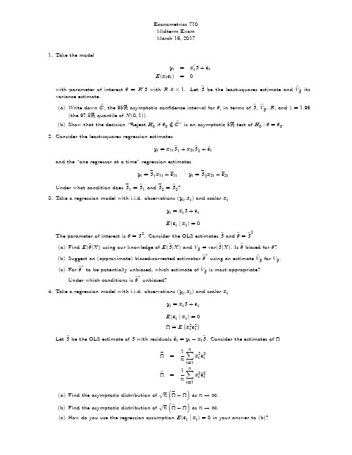
2. Consider the least-squares regression estimates
b , the 95% asymptotic con…dence interval for , in terms of b , V bb , R, and z = 1:96 (a) Write down C (the 97.5% quantile of N (0; 1)). b ” is an asymptotic 5% test of H0 : = 0 . (b) Show that the decision “Reject H0 if 0 2 =C yi = x1i b 1 + x2i b 2 + e bi yi = e 2 x2i + e e2i
and the “one regressor at a time” regression estimates yi = e 1 x1i + e e1i
3. Take a regression model with i.i.d. observations (yi ; xi ) and scalar xi yi = xi + ei E (ei j xi ) = 0
with resቤተ መጻሕፍቲ ባይዱduals e bi = yi b e =
1X 2 2 x e n i=1 i i 1X 2 2 x e b n i=1 i i
n
n
xi b . Consider the estimates of
= n e n b
(a) Find the asymptotic distribution of (b) Find the asymptotic distribution of
高级计量经济学试题final_2008a
2 3
distribution,
so
it
is
easy
to
conclude
that
the
observed
value of 3 is smaller than the critical value.
As alternative to the Wald statistic, you could compute the F statistic, and reject the hypothesis if the F statistic exceeds the 5% critical value from the F distribution with degrees of freedom (3,42). This is appropriate if you add the additional assumption that the error is independent of the regressors and Gaussian.
1 n
(y
1 n
(X 0 y Z )0
(y
X
0Z Z
) )
the GMM criterion is
Jn( ; 2) = ngn( ; 2)0 ^ 1gn( ; 2)
2;
and
^
=
1 n
Xn
g~ig~i0
i=1
! 1 Xn n g~i
i=1
1 Xn !0 n g~i
i=1
g~i = gi(~; ~2)
2 3
is
3,
so
the
observed
value
of
3 is certainly less than the 5% quantile. Alternatively, the 5% critical value of the
高级计量经济学(下)数据习 题、英文参考-第十八章
习 题建模练习题会要求对工资给付方程进行OLS 和2SLS 进行估计和分析,并且对整个联立方程组进行3SLS 估计。
1、试证明当线性约束(18-51)全部为排除约束时,方程识别的秩条件(18-56)和(18-50)等价。
2.验证第一节4方程例子的每个方程是否符合(18-59)秩条件。
3.试证明2SLS 估计量的一致性和渐进正态分布。
并推导其渐进分布。
4.试证明,在下面几种情形下,3SLS 和2SLS 是等价的。
1)∑是对角矩阵;2)每个方程都是恰好识别;3)系统的第m 个结构方程过度识别,而其余方程都是恰好识别,则对第m 个结构方程的2SLS 估计等价于3SLS ,(提示:参照Schmidt P. ,1976, Econometrics, New York: Marcel-Dekker)。
5.试证明定理3(提示:参照GMM 一章)。
6.试证明定理4(提示:参照GMM 一章)。
7.试证明权重矩阵(18-108)是最优的权重矩阵。
8.试容易证明基于权重矩阵n W (18-113)得到的GMM 估计量和基于权重矩阵n W (18-114)得到的最优GMM 等价的,两者都是渐进有效的GMM 估计量。
9.对于简约线性模型i i i y x βε=+,满足(())0i i i E y x β-=z 。
假设0β>。
写下GMM 标准函数()n S β。
重新定义参数使得1/θβ=,线性模型变为i i i x y θθε=-,正交条件可以写为(())0i i i E x y θ-=z ,写下GMM 标准函数()n S θ,采用相同的权重矩阵n W 。
是否能得出()(1/)n n S S ββ=,或(1/)()n n S S θθ=?10.证明FGLS 估计方法得到的非循环三角系统模型参数估计量是一致的估计量。
11.采用MORZ数据库对第六节例子中的工资给付方程进行分析。
(1)OLS回归结果如何?各系数的符号是否和期望相符?(2)2SLS回归结果如何?试与OLS回归结果进行比较。
计量经济学(英文版)
b1 + b2 x t
Assumptions of the Simple Linear Regression Model yt = b1 + b2x t + e t 2. E(e t) = 0 <=> E(yt) = b1 + b2x t
1.
3. var(e t)
4.3
=
4.
5.
cov(e i,e j)
yi and e i normally distributed
4.20
b2 = S wi yi
b1 = y - b2x
(x i - x) where wi = 2 S(x i - x)
This means that b1and b2 are normal since linear combinations of normals are normal.
2 2
(4.3b)
Variance of b2
4.12
Given that both yi and ei have variance s 2, the variance of the estimator b2 is:
var(b2) =
S(x i - x)
s2
2
b2 is a function of the yi values but var(b2) does not involve yi directly.
Gauss-Markov Theorem
4.16
Under the first five assumptions of the simple, linear regression model, the ordinary least squares estimators b1 and b2 have the smallest variance of all linear and unbiased estimators of b1 and b2. This means that b1and b2 are the Best Linear Unbiased Estimators (BLUE) of b1 and b2.
计量经济学练习题带答案版
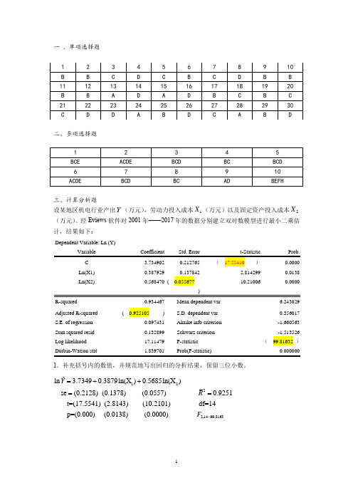
一 、单项选择题二、多项选择题三、计算分析题设某地区机电行业产出Y (万元),劳动力投入成本1X (万元)以及固定资产投入成本2X (万元)。
经Eviews 软件对2001年——2017年的数据分别建立双对数模型进行最小二乘估计,结果如下:Dependent Variable: Ln (Y)Ln(X1) 0.3879290.1378422.814299 0.0138 Ln(X2)0.568470 ( 0.05567710.210060.0000R-squared 0.934467 Mean dependent var6.243029 Adjusted R-squared ( 0.925105 ) S.D. dependent var0.356017 S.E. of regression 0.097431 Akaike info criterion -1.660563 Sum squared resid 0.132899 Schwarz criterion -1.513526 Log likelihood 17.11479 F-statistic ( 99.81632 )1.补充括号内的数值,并规范地写出回归的分析结果,保留三位小数。
122ˆln 3.73490.3879ln(X )0.5685ln(X ) se (0.2128) (0.1378) (0.0557) 0.9251t=(17.5541) (2.8143) (10.2101) df=14 p=(0.000) (0.0138)Y R =++==2,1499.8163(0.0000) F =2. 对模型的估计结果进行偏回归系数和整体显著性检验。
(t0.025(14)=2.145;t0.025(15)=2.131;F0.05(2,14)=3.74;F0.05(3,14)=3.34)。
(注意运用临界值法!!)样本量为17,临界值选取t0.025(14)=2.145F临界值选取F0.05(2,14)=3.743. 如果有两种可供选择的措施以提高机电行业产出,措施一是加大劳动力的投入,措施二是增大固定资产的投入,你认为哪个措施效果更明显,为什么?选择措施二,因为劳动力成本增长1个百分点,机电行业产增长0.39个百分点,而固定资产投入成本增长1个百分点,机电行业销售额仅增长0.57个百分点四、分析题根据我国31个细分制造业的数据,得到生产函数的如下估计结果:ln(Ŷi)=1.168+0.37ln(K i)+0.61ln(L i)se= (0.331) ( a) (0.1293)t= (3.53) ( 4.23) ( b )R2=0.94其中,Y为总产出,K为资本投入,L为劳动投入。
计量经济学试卷05
计量经济学 综合练习题(5)第一部分 选择题1、英文“Econometrics ”(计量经济学)一词最早是由挪威经济学家R .Frish 于( )年模仿“Biometrics ”(生物计量学)提出的。
A .1926B .1936C .1916D .19062、与经济学的其它分支学科相比,计量经济学家获得诺贝尔经济学奖的比重是( )。
A .占获奖总数的二分之一左右B .较低的C .占获奖总数的三分之二左右D .占获奖总数的三分之一左右3、关于计量经济学模型的检验,下列说法正确的是( )。
A .经济学准则检验又称一级检验,其他准则检验又称二级检验B .计量经济学准则检验又称一级检验,统计学准则检验又称二级检验C .计量经济学准则检验又称一级检验,实践准则检验又称模型事后检验D .统计学准则检验又称一级检验,计量经济学准则检验又称二级检验4、单方程模型中的变量可以分成( )两大类。
A .解释变量和虚拟变量;B .内生变量和外生变量C .内生变量和前定变量;D .内生变量和滞后变量5、在初级、中级计量经济学中常见的数据有横截面数据、( )和虚拟变量数据。
A .原始数据B .时间序列数据C .面板数据D .随机数据6、计量经济模型应用的四个主要方面分别是结构分析、经济预测、( )、检验和发展经济理论。
A .弹性分析B .经济政策评价C .乘数分析D .比较静力分析7、一元线性回归分析中,对于模型Y i = β0 + β1X i + u i 有A .nB .1C .n-1D .n-2其中 222ˆ,∑∑∑+=e y y i i i 。
) ( ˆ2的自由度为∑y i28、一元线性回归分析中,样本决定系数R 2=( )。
9、对于样本简单相关系数r ,以下结论中正确的是( )。
A .r 越近于1,说明变量之间负线性相关程度越高B .r 越近于0,说明变量之间线性相关程度越弱C .0≤r ≤1D .若r=0,则说明X 与Y 没有任何相关关系10、在满足基本假定的情况下,对单方程计量经济学模型而言,下列有关解释变量和被解释变量的说法中正确的是( )。
高级计量经济学试题mid_2016a

6=
5. The conditional mean is correctly speci…ed, so the least-squares estimators b = ( b 0 ; b 1 ; b 2 ) are unbiased for = (c0 ; c1 ; c2 ). b is a linear function of b . Since expectation is a linear operator b is therefore unbiased. More formally, E b =E b + 2b 1 2
x
1 n
Pn
i=1
1 1 p ei x e0 i i=1 x n P n 1 p ( x i i=1 n
Pn
i=1
x)
0
x ei x e0 i
1
0 1
1 X p ui n i=1
n
x ei ei
!
Notice that ui is iid, mean zero, and has variance Vu = E (ui u0 i) =
2 x
Ex2
= E (x
x) x 2 x x 3 x
2 3 x
= E x3 we …nd
2 x x:
2 x Ex :
+
2 x
and Ex3 = sx + 3
2 x x
+
cov x; x2 = sx + 3 Thus
1
+
3 x
2 x x
= sx + 2
= c1 + c2
sx + 2
2 x
高二英语经济指标单选题50题
高二英语经济指标单选题50题1. The GDP (Gross Domestic Product) of a country is calculated by adding up the value of all final goods and services produced ______ a given period.A. onB. inC. atD. for答案:B。
解析:本题考查介词在表示时间概念时的用法。
“in a given period”表示在一个特定的时期内,是计算GDP时常用的时间表达,所以B正确。
选项A“on”通常用于表示具体的某一天或日期;选项C“at”用于表示具体的时刻;选项D“for”强调持续的一段时间,但在这里表达在某个时期内,用“in”更合适。
2. CPI (Consumer Price Index) measures the average change over time in the prices paid by ______ consumers for a basket of goods and services.A. urbanB. ruralC. allD. foreign答案:A。
解析:CPI主要衡量的是城市消费者购买一篮子商品和服务的价格平均变化情况。
所以A正确。
选项B“rural”是农村的,与CPI主要关注的城市消费者不符;选项C“all”过于宽泛,没有体现出CPI重点关注的对象;选项D“foreign”外国的,与CPI的定义无关。
3. If a country's GDP growth rate is 3% this year and its population growth rate is 1%, then the per capita GDP growth rate is approximately ______.A. 1%B. 2%C. 3%D. 4%答案:B。
清华经管计量经济学习题3

1. Wooldridge (4th Ed) Ex 3.4. The following model is a simplified version of the multiple regression model used by Biddle and Hamermesh (1990) to study the tradeoff between time spent sleeping and working and to ... 2. Wooldridge (4th Ed) Ex 3.5. Consider the multiple regression model containing three independent variables, under Assumptions MLR. 1 through MLR. 4 ... 3. Wooldridge (4th Ed) Ex 3.6. In a study relating college grade point average to time spent in various activities, you distribute a survey to several students. The students are asked how many ... 4. Wooldridge (4th Ed) Ex 3.8 Which of the following can cause OLS estimators to be biased? ... 5. Wooldridge (4th Ed) Ex 3.12 (i) - (iii) (i) Consider the simple regression model y = β0 + β1 x + u under the first four Gauss-Markov assumptions. For some function g (x), for example ... 6. X1 ,X2 ,...,Xn ,... is a sequence of i.i.d. random variables with population mean µ and population variance σ 2 . Suppose that zero is NOT a value that Xn can possibly take. Prove that
高二英语经济学概念练习题30题含答案解析
高二英语经济学概念练习题30题含答案解析1.The law of demand states that as the price of a good increases, the quantity demanded _____.A.increasesB.decreasesC.remains the sameD.becomes zero答案解析:B。
根据需求定律,当商品价格上升时,需求量会减少。
选项A 增加不符合需求定律;选项C 保持不变也错误;选项D 变为零过于绝对。
本题涉及经济学中的需求定律概念,无特殊英语语法规则。
2.If the supply of a product decreases, what will happen to the price?A.It will increase.B.It will decrease.C.It will remain the same.D.It cannot be determined.答案解析:A。
当产品供给减少时,价格通常会上升。
因为供给减少,而需求相对稳定时,会出现供不应求的情况,导致价格上涨。
选项B 价格下降错误;选项C 保持不变不对;选项D 无法确定也不准确。
本题涉及经济学中的供给与价格关系概念,无特殊英语语法规则。
3.In a market economy, decisions about production and consumptionare mainly made by _____.A.the governmentB.businessesC.consumersD.the interaction of supply and demand答案解析:D。
在市场经济中,生产和消费的决策主要由供给和需求的相互作用决定。
选项A 政府不是主要决定者;选项B 企业只是供给方的一部分;选项C 消费者只是需求方的一部分。
本题涉及市场经济概念,无特殊英语语法规则。
经济学知识练习(英文)
经济学知识练习(英⽂)a. Please draw the demand curve.b. According to the demand curve, when price falls from point $40 to $30, please compute the price elasticity of demand using midpoint method. Is demand elastic or inelastic?c. What would happen to total revenue if price falls from $40 to $30?Which kind of relationship is there between the price elasticity of demand and total revenue? Answer: b. 7/5, elasticc. Increase total revenue by $1,000. Because demand is elastic, a decrease in the price causes an increase in the total revenue.b.Do you think recession(经济衰退)happens in 2008? Why?AnswerAnswer questions regarding pork market.a. How can a tax on pork(猪⾁)influence the pork’s demand curve? Please answer and explain.b. If the price of beef decreases, how will the demand of pork change? What are the changes in equilibrium price and quantity? Please graph(图⽰)the change. .c. Please list factors may increase the demand of pork. Answers:a.The demand curve will not change. A tax can make the price of pork to be higher, but the higher price can not make any changes about the curve.b.Demand of pork will decrease. Because pork and beef are substitute, a lower price of beef will decrease the demand of pork. Equilibrium price will decrease and equilibrium quantity will decrease too.c.to increase the prices of its substitutes; to decrease the taxes on pork……(consider the determinants of demand)normal good or an inferior good(低档物品)? Why do you think so?b.According to the table, is Good X a normal good or an inferior good? Why do you think so?Answer:a. –2.33, an inferior good, because Good Y’s income elasticity is negative, and increase in income has caused an decrease in the quantity demanded for it.b. A normal good, because Good X’s income ela sticity is positive, the increase in income has caused an increase in the quantity demanded for itSuppose the book market is competitive. All the firms have the same cost. Each firm has fixed cost of $160, and averageQuestion:/doc/86df1121bcd126fff7050b56.html pute marginal cost and average total cost.b.Now the price is $90. How many books each firm produce to maximize the profit?c.Is this industry in long-run equilibrium? Why or why not? Answer: 1)3) NO. because now price(90) and minimum of ATC (80) are not equal, or profit is not 0. Tom owns a small factory that produces electrical fans. So far, he’s sold 500 units of the products and faces the following6. Jim and Tom meet George, the banker, to work out the details of a mortgage. They all expect that inflation will be 2 percent over the term of the loan, and they agree on a nominal interest rate of 6 percent. As it turns out, the inflation rate is5 percent over the term of the loan.a. What was the expected real interest rate?b. What was the actual real interest rate?c.Who benefited and who lost because of the unexpected inflation?Answera. 6-2=4b. 6-5=1c. Jim and Tom benefited and George lost.7. Answer questions regarding pork market.a. How can a tax o n pork influence the pork’s demand curve? Please answer and explain.b. If there is a new and better technology used on breeding pigs, how will the supply of pork change? What are the changes in equilibrium price and quantity? Please graph (图⽰)the change.c. Please list factors may increase the supply of pork. Answers:(1)It’s the claim that, other things equal, the quantity demanded of a good decreases when the price of the good rises.(2)The demand curve will not change. A tax can make the price of pork to be higher, but the higher price can not make any changes about the curve.(3)Supply of pork will increase. Equilibrium price will decrease and equilibrium quantity will increase.(4)to research some new technology; to decrease the prices of inputs ……(consider the determinants of supply) 8. Explain how each of the following events shifts the short-run aggregate-supply curve or the aggregate-demand curve and what are the effects on output and the price level.a. The stock market declines sharply, reducing consumers’ wealth.b. The price of crude oil rises.c. A technological improvement raises productivity.d. Government decreases spending on national defense.Answer:a.short-run aggregate –demand curve shifts to the left, price down and output decrease.b.Short-run aggregate-supply curve shifts to the left, price up and output decrease.c.Short-run and long-run aggregate-supply curve shifts to the right, price down and output increase.d.short-run aggregate –demand curve shifts to the left, price down and output decrease.。
计量经济学精要练习题1

1、将内生变量的前期值作解释变量,这样的变量称为()
A.虚拟变量B.控制变量
C.政策变量D.滞后变量
2、半对数模型 中,参数 的含义是()
A.X的绝对量发生一定变动时,引起因变量Y的相对变化率
B.Y关于X的弹性
C.X的相对变化,引起Y的期望值绝对量变化
D.Y关于X的边际变化
3、设OLS法得到的样本回归直线为 ,则点 ()
VariableCoefficientStd. Error T-StatisticProb.
C24.40706.9973 ________ 0.0101
0.34010.4785________0.5002
-0.0823 0.04580.1152
R-squared
Adjusted R-squaredVariance of Y12365.44
11.对于原模型 ,广义差分模型是指()。
A.
B.
C.
D.
12.下列哪种形式的序列相关可用DW统计量来检验( 为具有零均值,同方差,且不存在序列相关的随机变量)( )。
A. B.
C. D.
13.假定在已知某企业生产的产品具有明显的季节特征的情况下,该企业生产决策由模型 描述(其中 为产量, 为价格)。则该模型将存在()。
C模型:
Dependent Variable: CHD
Method: Least Squares
Included observations: 34
Variable
Coefficient
Std. Error
t-Statistic
Prob.
CIG
10.70566
4.
2.
0.0268
- 1、下载文档前请自行甄别文档内容的完整性,平台不提供额外的编辑、内容补充、找答案等附加服务。
- 2、"仅部分预览"的文档,不可在线预览部分如存在完整性等问题,可反馈申请退款(可完整预览的文档不适用该条件!)。
- 3、如文档侵犯您的权益,请联系客服反馈,我们会尽快为您处理(人工客服工作时间:9:00-18:30)。
ECONOMETRIC METHODS (U20451)ASSIGNMENT, FEBRUARY 2014An Excel file has been uploaded on the Moodle site for the unit, which is entitled ‘Assignment Data’. This file contains annual data from 1994 to 2012 on three variables:Y = purchases of vehicles in the UK (constant prices);X = UK real household disposable income;Z = an EU measure of consumer confidence for the UK.Please copy the data from the Excel file into an EViews workfile.Descriptive Element (10 marks)Produce a line graph of each of the time series. Using no more than 200 words, describe the behaviour of each of the variables over the nineteen-year period.Two-Variable Linear Regression Model (20 marks)There is presented below a population regression function:Y t = B0 + B1X t + u t, t = 1994, 1995, ………, 2012.B0 and B1 are population parameters. u t denotes a random disturbance term.Assume that E[u t] = 0, t = 1994, 1995, ………, 2012.Proceed to provide interpretations of the population parameters.Apply Ordinary Least Squares estimation to the population regression function.Indicate the point estimates of the two parameters.Proceed to produce a 95 per cent confidence interval for B1, explaining the manner of its construction.Adopting two different approaches (i.e., consulting the statistical table and using the probability value), perform a test of null hypothesis, Ho: B1= 0, against the alternative hypothesis, Ha: B1≠ 0.The validity of the confidence interval and the test of the hypothesis rests partly on the disturbance terms being normally distributed.Adopting two different approaches (i.e., consulting the statistical table and using the probability value), perform a suitable test in order to assess whether or not the disturbance terms are normally distributed.Three-Variable Linear Regression Model (25 marks)There is presented below a three-variable population regression function:Y = B0 + B1X t + B2Z t + u t, t = 1994, 1995, ………, 2012.(B2 is a population parameter.)Assuming that E[u t] = 0, t = 1994, 1995, ………, 2012, provide an interpretation of each of the population parameters.Apply to the regression equation Ordinary Least Squares estimation.Adopting two different approaches (i.e., consulting the statistical table and using the probability value), perform a test of the joint hypothesis, Ho: B1= 0, B2= 0, against the alternative hypothesis, Ha: at least one of B1≠ 0, B2≠ 0With respect to the estimated versions of the two- and three-variable regression functions, compare the values of each of the following statistics:- The residual sum of squares;- The coefficient of determination;- The standard error of the regression;- The adjusted R-squared statistic.Account for the change in the value of each of the statistics in moving from the two- to the three-variable regression equation.Three-Variable Log-Linear Regression Model (20 marks)Alternative specificationlog.(Y t) = B0 + B1log.(X t) + B2Z t + u t, t = 1994, 1995, ………, 2012.Explain why a logarithmic transformation was not applied to the variable, Z.Provide an interpretation of each of B1 and B2.Apply to the logarithmic model Ordinary Least Squares estimation.In terms of the fit of the sample data on Y, how does the three-variable log-linear model compare with the three-variable linear specification?An Extension of the Three-Variable Linear Regression Model (15 marks)Consider, once again, the three-variable linear regression equation:Y t = B0 + B1X t + B2Z t + u t, t = 1994, 1995, ………, 2012.The previous Labour Government implemented a car scrappage scheme in 2009 that was intended to encourage the purchase of new cars. The suggestion has been made that this policy had the effect of redistributing expenditure on vehicles, specifically, making this higher than it would otherwise have been in 2009 but lower than it would otherwise have been in 2010.Construct two dichotomous/dummy variables to capture these effects and add them to the above model as explanatory variables.Estimate the extended model using Ordinary Least Squares. On the basis of the estimation output that is produced by EViews, is there statistical evidence to support the contention that a redistribution of vehicle purchases occurred?Limitations of the Regression Models (10 marks)On the basis of your knowledge of the factors that determine household expenditure on durable goods, suggest some further explanatory variables that possibly should have entered this analysis.For the purpose of undertaking this assignment, students are permitted to work either individually or in the form of a pair. If two students are officially working together then please ensure to show both of the student numbers.Given the quantitative nature of the assignment then no word limit is applicable.Submission Date: 25th April 2014Robert Gausden, February 2014。