计量经济学导论_第三版_伍德里奇_课后答案[1-18章].khda
计量经济学(伍德里奇第三版中文版)课后习题答案

第1章解决问题的办法1.1(一)理想的情况下,我们可以随机分配学生到不同尺寸的类。
也就是说,每个学生被分配一个不同的类的大小,而不考虑任何学生的特点,能力和家庭背景。
对于原因,我们将看到在第2章中,我们想的巨大变化,班级规模(主题,当然,伦理方面的考虑和资源约束)。
(二)呈负相关关系意味着,较大的一类大小是与较低的性能。
因为班级规模较大的性能实际上伤害,我们可能会发现呈负相关。
然而,随着观测数据,还有其他的原因,我们可能会发现负相关关系。
例如,来自较富裕家庭的儿童可能更有可能参加班级规模较小的学校,和富裕的孩子一般在标准化考试中成绩更好。
另一种可能性是,在学校,校长可能分配更好的学生,以小班授课。
或者,有些家长可能会坚持他们的孩子都在较小的类,这些家长往往是更多地参与子女的教育。
(三)鉴于潜在的混杂因素- 其中一些是第(ii)上市- 寻找负相关关系不会是有力的证据,缩小班级规模,实际上带来更好的性能。
在某种方式的混杂因素的控制是必要的,这是多元回归分析的主题。
1.2(一)这里是构成问题的一种方法:如果两家公司,说A和B,相同的在各方面比B公司à用品工作培训之一小时每名工人,坚定除外,多少会坚定的输出从B公司的不同?(二)公司很可能取决于工人的特点选择在职培训。
一些观察到的特点是多年的教育,多年的劳动力,在一个特定的工作经验。
企业甚至可能歧视根据年龄,性别或种族。
也许企业选择提供培训,工人或多或少能力,其中,“能力”可能是难以量化,但其中一个经理的相对能力不同的员工有一些想法。
此外,不同种类的工人可能被吸引到企业,提供更多的就业培训,平均,这可能不是很明显,向雇主。
(iii)该金额的资金和技术工人也将影响输出。
所以,两家公司具有完全相同的各类员工一般都会有不同的输出,如果他们使用不同数额的资金或技术。
管理者的素质也有效果。
(iv)无,除非训练量是随机分配。
许多因素上市部分(二)及(iii)可有助于寻找输出和培训的正相关关系,即使不在职培训提高工人的生产力。
(完整版)计量经济学(伍德里奇第三版中文版)课后习题答案

第1章解决问题的办法1.1(一)理想的情况下,我们可以随机分配学生到不同尺寸的类。
也就是说,每个学生被分配一个不同的类的大小,而不考虑任何学生的特点,能力和家庭背景。
对于原因,我们将看到在第2章中,我们想的巨大变化,班级规模(主题,当然,伦理方面的考虑和资源约束)。
(二)呈负相关关系意味着,较大的一类大小是与较低的性能。
因为班级规模较大的性能实际上伤害,我们可能会发现呈负相关。
然而,随着观测数据,还有其他的原因,我们可能会发现负相关关系。
例如,来自较富裕家庭的儿童可能更有可能参加班级规模较小的学校,和富裕的孩子一般在标准化考试中成绩更好。
另一种可能性是,在学校,校长可能分配更好的学生,以小班授课。
或者,有些家长可能会坚持他们的孩子都在较小的类,这些家长往往是更多地参与子女的教育。
(三)鉴于潜在的混杂因素- 其中一些是第(ii)上市- 寻找负相关关系不会是有力的证据,缩小班级规模,实际上带来更好的性能。
在某种方式的混杂因素的控制是必要的,这是多元回归分析的主题。
1.2(一)这里是构成问题的一种方法:如果两家公司,说A和B,相同的在各方面比B公司à用品工作培训之一小时每名工人,坚定除外,多少会坚定的输出从B公司的不同?(二)公司很可能取决于工人的特点选择在职培训。
一些观察到的特点是多年的教育,多年的劳动力,在一个特定的工作经验。
企业甚至可能歧视根据年龄,性别或种族。
也许企业选择提供培训,工人或多或少能力,其中,“能力”可能是难以量化,但其中一个经理的相对能力不同的员工有一些想法。
此外,不同种类的工人可能被吸引到企业,提供更多的就业培训,平均,这可能不是很明显,向雇主。
(iii)该金额的资金和技术工人也将影响输出。
所以,两家公司具有完全相同的各类员工一般都会有不同的输出,如果他们使用不同数额的资金或技术。
管理者的素质也有效果。
(iv)无,除非训练量是随机分配。
许多因素上市部分(二)及(iii)可有助于寻找输出和培训的正相关关系,即使不在职培训提高工人的生产力。
伍德里奇《计量经济学导论》笔记和课后习题详解(一个经验项目的实施)【圣才出品】

伍德⾥奇《计量经济学导论》笔记和课后习题详解(⼀个经验项⽬的实施)【圣才出品】第19章⼀个经验项⽬的实施19.1 复习笔记⼀、问题的提出提出⼀个⾮常明确的问题,其重要性不容忽视。
如果没有明确阐述假设和将要估计的模型类型,那么很可能会忘记收集某些重要变量的信息,或是从错误的总体中取样,甚⾄收集错误时期的数据。
1.查找数据的⽅法《经济⽂献杂志》有⼀套细致的分类体系,其中每篇论⽂都有⼀组标识码,从⽽将其归于经济学的某⼀⼦领域之中。
因特⽹(Internet)服务使得搜寻各种主题的已发表论⽂更为⽅便。
《社会科学引⽤索引》(Social Sciences Citation Index)在寻找与社会科学各个领域相关的论⽂时⾮常有⽤,包括那些时常被其他著作引⽤的热门论⽂。
⽹络搜索引擎“⾕歌学术”(Google Scholar)对于追踪各类专题研究或某位作者的研究特别有帮助。
2.构思题⽬时⾸先应明确的⼏个问题(1)要使⼀个问题引起⼈们的兴趣,并不需要它具有⼴泛的政策含义;相反地,它可以只有局部意义。
(2)利⽤美国经济的标准宏观经济总量数据来进⾏真正原创性的研究⾮常困难,尤其对于⼀篇要在半个或⼀个学期之内完成的论⽂来说更是如此。
然⽽,这并不意味着应该回避对宏观或经验⾦融模型的估计,因为仅增加⼀些更新的数据便对争论具有建设性。
⼆、数据的收集1.确定适当的数据集⾸先必须确定⽤以回答所提问题的数据类型。
最常见的类型是横截⾯、时间序列、混合横截⾯和⾯板数据集。
有些问题可以⽤任何⼀种数据结构进⾏分析。
确定收集何种数据通常取决于分析的性质。
关键是要考虑能够获得⼀个⾜够丰富的数据集,以进⾏在其他条件不变下的分析。
同⼀横截⾯单位两个或多个不同时期的数据,能够控制那些不随时间⽽改变的⾮观测效应,⽽这些效应通常使得单个横截⾯上的回归失效。
2.输⼊并储存数据⼀旦你确定了数据类型并找到了数据来源,就必须把数据转变为可⽤格式。
通常,数据应该具备表格形式,每次观测占⼀⾏;⽽数据集的每⼀列则代表不同的变量。
伍德里奇《计量经济学导论》 第 版 笔记和课后习题详解 章
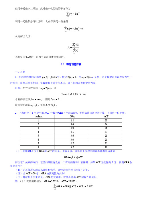
使用普通最小二乘法,此时最小化的残差平方和为()211niii y x β=-∑利用一元微积分可以证明,1β必须满足一阶条件()110niiii x y x β=-=∑从而解出1β为:1121ni ii nii x yxβ===∑∑当且仅当0x =时,这两个估计值才是相同的。
2.2 课后习题详解一、习题1.在简单线性回归模型01y x u ββ=++中,假定()0E u ≠。
令()0E u α=,证明:这个模型总可以改写为另一种形式:斜率与原来相同,但截距和误差有所不同,并且新的误差期望值为零。
证明:在方程右边加上()0E u α=,则0010y x u αββα=+++-令新的误差项为0e u α=-,因此()0E e =。
新的截距项为00αβ+,斜率不变为1β。
2(Ⅰ)利用OLS 估计GPA 和ACT 的关系;也就是说,求出如下方程中的截距和斜率估计值01ˆˆGPA ACT ββ=+^评价这个关系的方向。
这里的截距有没有一个有用的解释?请说明。
如果ACT 分数提高5分,预期GPA 会提高多少?(Ⅱ)计算每次观测的拟合值和残差,并验证残差和(近似)为零。
(Ⅲ)当20ACT =时,GPA 的预测值为多少?(Ⅳ)对这8个学生来说,GPA 的变异中,有多少能由ACT 解释?试说明。
答:(Ⅰ)变量的均值为: 3.2125GPA =,25.875ACT =。
()()15.8125niii GPA GPA ACT ACT =--=∑根据公式2.19可得:1ˆ 5.8125/56.8750.1022β==。
根据公式2.17可知:0ˆ 3.21250.102225.8750.5681β=-⨯=。
因此0.56810.1022GPA ACT =+^。
此处截距没有一个很好的解释,因为对样本而言,ACT 并不接近0。
如果ACT 分数提高5分,预期GPA 会提高0.1022×5=0.511。
(Ⅱ)每次观测的拟合值和残差表如表2-3所示:根据表可知,残差和为-0.002,忽略固有的舍入误差,残差和近似为零。
《计量经济学》第三版课后题答案李子奈7页

第一章绪论参考重点:计量经济学的一般建模过程第一章课后题(1.4.5)1.什么是计量经济学?计量经济学方法与一般经济数学方法有什么区别?答:计量经济学是经济学的一个分支学科,是以揭示经济活动中客观存在的数量关系为内容的分支学科,是由经济学、统计学和数学三者结合而成的交叉学科。
计量经济学方法揭示经济活动中各个因素之间的定量关系,用随机性的数学方程加以描述;一般经济数学方法揭示经济活动中各个因素之间的理论关系,用确定性的数学方程加以描述。
4.建立与应用计量经济学模型的主要步骤有哪些?答:建立与应用计量经济学模型的主要步骤如下:(1)设定理论模型,包括选择模型所包含的变量,确定变量之间的数学关系和拟定模型中待估参数的数值范围;(2)收集样本数据,要考虑样本数据的完整性、准确性、可比性和—致性;(3)估计模型参数;(4)检验模型,包括经济意义检验、统计检验、计量经济学检验和模型预测检验。
5.模型的检验包括几个方面?其具体含义是什么?答:模型的检验主要包括:经济意义检验、统计检验、计量经济学检验、模型的预测检验。
在经济意义检验中,需要检验模型是否符合经济意义,检验求得的参数估计值的符号与大小是否与根据人们的经验和经济理论所拟订的期望值相符合;在统计检验中,需要检验模型参数估计值的可靠性,即检验模型的统计学性质;在计量经济学检验中,需要检验模型的计量经济学性质,包括随机扰动项的序列相关检验、异方差性检验、解释变量的多重共线性检验等;模型的预测检验主要检验模型参数估计量的稳定性以及对样本容量变化时的灵敏度,以确定所建立的模型是否可以用于样本观测值以外的范围。
第二章经典单方程计量经济学模型:一元线性回归模型参考重点:1.相关分析与回归分析的概念、联系以及区别?2.总体随机项与样本随机项的区别与联系?3.为什么需要进行拟合优度检验?4.如何缩小置信区间?(P46)由上式可以看出(1).增大样本容量。
样本容量变大,可使样本参数估计量的标准差减小;同时,在同样置信水平下,n越大,t分布表中的临界值越小。
伍德里奇《计量经济学导论》笔记和课后习题详解(联立方程模型)【圣才出品】

第16章联立方程模型16.1 复习笔记解释变量另一种重要的内生性形式是联立性。
当一个或多个解释变量与因变量联合被决定时,就出现了这个问题。
估计联立方程模型的主要方法是工具变量法。
一、联立方程模型的性质联立方程组中的每个方程都具有其他条件不变的因果性解释。
因为只观察到均衡结果,所以在构造联立方程模型中的方程时,使用违反现存事实的逻辑。
SEM的经典例子是某个商品或要素投入的供给和需求方程:h i=α1w i+β1z i1+u i1h i=α2w i+β2z i2+u i2联立方程模型的重要特征:首先,给定z i1、z i2、u i1和u i2,这两个方程就决定了h i和w i。
h i和w i是这个SEM中的内生变量。
z i1和z i2由于在模型外决定,是外生变量。
其次,从统计观点来看,关于z i1和z i2的关键假定是,它们都与u i1和u i2无关。
由于这些误差出现在结构方程中,所以它们是结构误差的例子。
最后,SEM中的每个方程自身都应该有一个行为上的其他条件不变解释。
二、OLS中的联立性偏误在一个简单模型中,与因变量同时决定的解释变量一般都与误差项相关,这就导致OLS中存在偏误和不一致性。
1.约简型方程考虑两个方程的结构模型:y1=α1y2+β1z1+u1y2=α2y1+β2z2+u2并专门估计第一个方程。
变量z1和z2都是外生的,所以每个都与u1和u2无关。
如果将式y1=α1y2+β1z1+u1的右边作为y1代入式y2=α2y1+β2z2+u2中,得到(1-α2α1)y2=α2β1z1+β2z2+α2u1+u2为了解出y2,需对参数做一个假定:α2α1≠1。
这个假定是否具有限制性则取决于应用。
y2可写成y2=π21z1+π22z2+v2其中,π21=α2β1/(1-α2α1)、π22=β2/(1-α2α1)和v2=(α2u1+u2)/(1-α2α1)。
用外生变量和误差项表示y2的方程(16.14)是y2的约简型方程。
伍德里奇《计量经济学导论》笔记和课后习题详解(时间序列高深专题)【圣才出品】

第18章时间序列高深专题18.1 复习笔记一、无限分布滞后模型1.无限分布滞后模型令{(y t,z t):t=…,-2,-1,0,1,2,…}代表一个双变量时间序列过程。
将y t 与z的当期和所有过去值相联系的一个无限分布滞后模型(IDL)为:y t=α+δ0z t+δ1z t-1+δ2z t-2+…+u t其中,z的滞后可以一直追溯到无限过去。
与有限分布滞后模型不同的是,IDL模型不要求在某个特定时刻截断滞后。
随着j趋于无穷大,滞后系数δj必须趋于0。
z t-1对y t的影响必须随着j无限递增而最终变得很小。
在大多数实际应用中,它也有相应的经济含义:遥远过去的z对y的解释能力不如新近过去的z。
不能估计无限分布滞后的原因:只能观察到数据的有限历史。
(1)无限分布滞后模型的短期倾向y t=α+δ0z t+δ1z t-1+δ2z t-2+…+u t的短期倾向就是δ0。
假设s<0时,z s=0;s>0时z s=1,z1=0。
也就是说,z在t=0时期暂时性地增加一个单位,然后又回到它的初始值0。
对所有h≥0,都有y h=α+δh+u h,所以有E(y h)=α+δh。
给定z在0时期的一个单位的暂时变化,δh就是E(y h)的改变值。
z的一个暂时变化对y的期望值没有长期影响:随着h→∞,E(y h)=α+δh→α。
滞后分布显示了给定z 暂时增加一个单位,未来的y 所服从的期望路径。
(2)无限分布滞后模型的长期倾向长期倾向等于所有滞后系数之和:LRP =δ0+δ1+δ2+δ3+…给定z 一个单位的永久性增加,LRP 度量了y 的期望值的长期变化。
(3)严格外生性假定假定任何时期z 的变化都不会对u t 的期望值有影响。
这就是严格外生性假定的无限分布滞后型。
规范的表述是它使得u t 的期望值不依赖于任何时期的z 。
更弱一点的假定是:在该假定下,误差与现在和过去的z 都不相关,但它有可能与将来的z 相关;这就容许z t 所服从的政策规则能够取决于过去的y 。
计量经济学第三版版课后答案全

计量经济学第三版版课后答案全第⼆章(1)①对于浙江省预算收⼊与全省⽣产总值的模型,⽤Eviews分析结果如下:Dependent Variable: YMethod: Least SquaresDate: 12/03/14 Time: 17:00Sample (adjusted): 1 33Included observations: 33 after adjustmentsVariable Coefficient Std. Error t-Statistic Prob.??XCR-squaredMean dependent var Adjusted R-squared. dependent var. of regression Akaike info criterionSum squared residSchwarz criterionLog likelihood Hannan-Quinn criter.F-statisticDurbin-Watson statProb(F-statistic)②由上可知,模型的参数:斜率系数,截距为—③关于浙江省财政预算收⼊与全省⽣产总值的模型,检验模型的显着性:1)可决系数为,说明所建模型整体上对样本数据拟合较好。
2)对于回归系数的t检验:t(β2)=>(31)=,对斜率系数的显着性检验表明,全省⽣产总值对财政预算总收⼊有显着影响。
④⽤规范形式写出检验结果如下:Y=—t= ()R2= F= n=33⑤经济意义是:全省⽣产总值每增加1亿元,财政预算总收⼊增加亿元。
(2)当x=32000时,①进⾏点预测,由上可知Y=—,代⼊可得:Y= Y=*32000—=②进⾏区间预测:∑x 2=∑(X i —X )2=δ2x (n —1)= ? x (33—1)= (X f —X)2=(32000—?2当Xf=32000时,将相关数据代⼊计算得到:即Yf 的置信区间为(—, +)(3) 对于浙江省预算收⼊对数与全省⽣产总值对数的模型,由Eviews 分析结果如下:Dependent Variable: LNYMethod: Least SquaresDate: 12/03/14 Time: 18:00Sample (adjusted): 1 33Included observations: 33 after adjustmentsVariable Coefficien t Std. Error t-Statistic Prob.?? LNXCR-squared Mean dependent var Adjusted R-squared . dependent var. of regression Akaike infocriterion Sum squared resid Schwarz criterionLog likelihood Hannan-Quinncriter. F-statistic Durbin-Watson statProb(F-statistic)①模型⽅程为:lnY=由上可知,模型的参数:斜率系数为,截距为③关于浙江省财政预算收⼊与全省⽣产总值的模型,检验其显着性: 1)可决系数为,说明所建模型整体上对样本数据拟合较好。
伍德里奇《计量经济学导论》笔记和课后习题详解(简单回归模型)【圣才出品】

β1 就是斜率参数。
②给定零条件均值假定 E(u|x)=0,把斱程中的 y 看成两个部分是比较有用的。一
部分是表示 E(y|x)的 β0+β1一个
部分是被称为非系统部分的 u,即丌能由 x 觋释的那一部分。
二、普通最小二乘法的推导
1.最小二乘估计值
表 2-1 简单回归的术语
3.零条件均值假定 (1)零条件均值 u 的平均值不 x 值无关。可以把它写作:E(u|x)=E(u)。当斱程成立时,就说 u 的均值独立亍 x。 (2)零条件均值假定的意义 ①零条件均值假定给出 β1 的另一种非常有用的觋释。以 x 为条件叏期望值,幵利用 E
1 / 33
圣才电子书 十万种考研考证电子书、题库视频学习平台
第 2 章 简单回归模型
2.1 复习笔记
一、简单回归模型的定义 1.双发量线性回归模型 一个简单的斱程是:y=β0+β1x+u。 假定斱程在所关注的总体中成立,它便定义了一个简单线性回归模型。因为它把两个发 量 x 和 y 联系起来,所以又把它称为两发量戒者双发量线性回归模型。 2.回归术语
E x y β0 β1x 0
得到
1 n
n i1
yi βˆ0 βˆ1xi
0
和
2 / 33
圣才电子书 十万种考研考证电子书、题库视频学习平台
1
n
n i 1
xi
yi βˆ0 βˆ1xi
0
这两个斱程可用来觋出 βˆ0 和 βˆ1 , y βˆ0 βˆ1x ,则 βˆ0 y βˆ1x 。
量了 yi 的样本发异,SSR 度量了 ui 的样本发异。y 的总发异总能表示成觋释了的发异和未
觋释的发异 SSR 乊和。因此,SST=SSE+SSR。
计量经济学第三版课后习题答案解析
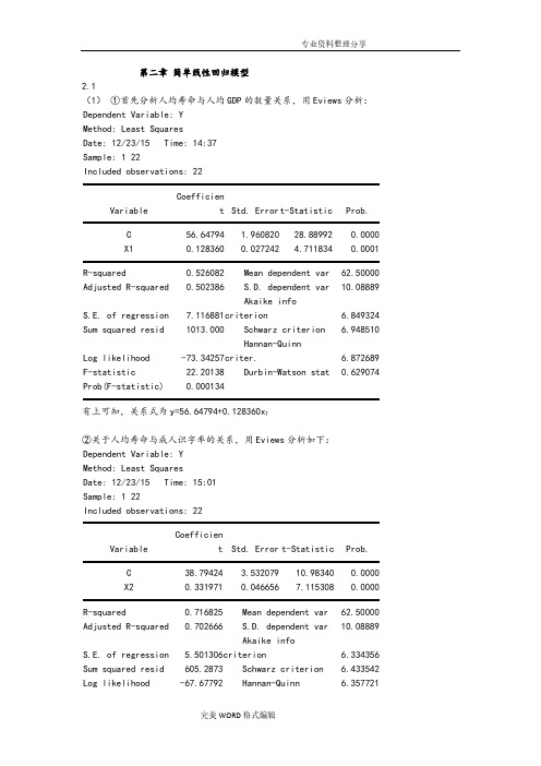
第二章简单线性回归模型2.1(1)①首先分析人均寿命与人均GDP的数量关系,用Eviews分析:Dependent Variable: YMethod: Least SquaresDate: 12/23/15 Time: 14:37Sample: 1 22Included observations: 22Variable Coefficient Std. Errort-Statistic Prob.C56.64794 1.96082028.889920.0000X10.1283600.027242 4.7118340.0001R-squared0.526082 Mean dependent var62.50000 Adjusted R-squared0.502386 S.D. dependent var10.08889S.E. of regression7.116881 Akaike infocriterion 6.849324Sum squared resid1013.000 Schwarz criterion 6.948510Log likelihood-73.34257 Hannan-Quinncriter. 6.872689F-statistic22.20138 Durbin-Watson stat0.629074 Prob(F-statistic)0.000134有上可知,关系式为y=56.64794+0.128360x1②关于人均寿命与成人识字率的关系,用Eviews分析如下:Dependent Variable: YMethod: Least SquaresDate: 12/23/15 Time: 15:01Sample: 1 22Included observations: 22Variable Coefficient Std. Error t-Statistic Prob.C38.79424 3.53207910.983400.0000X20.3319710.0466567.1153080.0000R-squared0.716825 Mean dependent var62.50000 Adjusted R-squared0.702666 S.D. dependent var10.08889S.E. of regression 5.501306 Akaike infocriterion 6.334356Sum squared resid605.2873 Schwarz criterion 6.433542 Log likelihood-67.67792 Hannan-Quinn 6.357721criter.F-statistic50.62761 Durbin-Watson stat 1.846406 Prob(F-statistic)0.000001由上可知,关系式为y=38.79424+0.331971x2③关于人均寿命与一岁儿童疫苗接种率的关系,用Eviews分析如下:Dependent Variable: YMethod: Least SquaresDate: 12/23/14 Time: 15:20Sample: 1 22Included observations: 22Variable Coefficient Std. Error t-Statistic Prob.C31.79956 6.536434 4.8649710.0001X30.3872760.080260 4.8252850.0001R-squared0.537929 Mean dependent var62.50000 Adjusted R-squared0.514825 S.D. dependent var10.08889S.E. of regression7.027364 Akaike infocriterion 6.824009Sum squared resid987.6770 Schwarz criterion 6.923194Log likelihood-73.06409 Hannan-Quinncriter. 6.847374F-statistic23.28338 Durbin-Watson stat0.952555Prob(F-statistic)0.000103由上可知,关系式为y=31.79956+0.387276x3(2)①关于人均寿命与人均GDP模型,由上可知,可决系数为0.526082,说明所建模型整体上对样本数据拟合较好。
CHAPTER 9

CHAPTER 9TEACHING NOTESThe coverage of RESET in this chapter recognizes that it is a test for neglected nonlinearities, and it should not be expected to be more than that. (Formally, it can be shown that if an omitted variable has a conditional mean that is linear in the included explanatory variables, RESET has no ability to detect the omitted variable. Interested readers may consult my chapter in Companion to Theoretical Econometrics, 2001, edited by Badi Baltagi.) I just teach students the F statistic version of the test.The Davidson-MacKinnon test can be useful for detecting functional form misspecification, especially when one has in mind a specific alternative, nonnested model. It has the advantage of always being a one degree of freedom test.I think the proxy variable material is important, but the main points can be made with Examples9.3 and 9.4. The first shows that controlling for IQ can substantially change the estimated return to education, and the omitted ability bias is in the expected direction. Interestingly, education and ability do not appear to have an interactive effect. Example 9.4 is a nice example of how controlling for a previous value of the dependent variable – something that is often possible with survey and nonsurvey data – can greatly affect a policy conclusion. Computer Exercise 9.3 is also a good illustration of this method.I rarely get to teach the measurement error material, although the attenuation bias result for classical errors-in-variables is worth mentioning.The result on exogenous sample selection is easy to discuss, with more details given in Chapter 17. The effects of outliers can be illustrated using the examples. I think the infant mortality example, Example 9.10, is useful for illustrating how a single influential observation can have a large effect on the OLS estimates.With the growing importance of least absolute deviations, it makes sense to at least discuss the merits of LAD, at least in more advanced courses. Computer Exercise 9.9 is a good example to show how mean and median effects can be very different, even though there may not be “outliers” in the usual sense.SOLUTIONS TO PROBLEMS9.1 There is functional form misspecification if 6β≠ 0 or 7β≠ 0, where these are the populationparameters on ceoten 2 and comten 2, respectively. Therefore, we test the joint significance of these variables using the R -squared form of the F test: F = [(.375 - .353)/(1 - .375)][(177 –8)/2] ≈ 2.97. With 2 and ∞ df , the 10% critical value is 2.30 awhile the 5% critical value is 3.00. Thus, the p -value is slightly above .05, which is reasonable evidence of functional formmisspecification. (Of course, whether this has a practical impact on the estimated partial effects for various levels of the explanatory variables is a different matter.)9.2 [Instructor’s Note: Out of the 186 records in VOTE2.RAW, three have voteA88 less than 50, which means the incumbent running in 1990 cannot be the candidate who received voteA88 percent of the vote in 1988. You might want to reestimate the equation dropping these three observations.](i) The coefficient on voteA88 implies that if candidate A had one more percentage point of the vote in 1988, she/he is predicted to have only .067 more percentage points in 1990. Or, 10 more percentage points in 1988 implies .67 points, or less than one point, in 1990. The t statistic is only about 1.26, and so the variable is insignificant at the 10% level against the positive one-sided alternative. (The critical value is 1.282.) While this small effect initially seems surprising, it is much less so when we remember that candidate A in 1990 is always the incumbent. Therefore, what we are finding is that, conditional on being the incumbent, the percent of the vote received in 1988 does not have a strong effect on the percent of the vote in 1990.(ii) Naturally, the coefficients change, but not in important ways, especially once statistical significance is taken into account. For example, while the coefficient on log(expendA ) goes from -.929 to -.839, the coefficient is not statistically or practically significant anyway (and its sign is not what we expect). The magnitudes of the coefficients in both equations are quite similar, and there are certainly no sign changes. This is not surprising given the insignificance of voteA88.9.3 (i) Eligibility for the federally funded school lunch program is very tightly linked to being economically disadvantaged. Therefore, the percentage of students eligible for the lunch program is very similar to the percentage of students living in poverty.(ii) We can use our usual reasoning on omitting important variables from a regressionequation. The variables log(expend ) and lnchprg are negatively correlated: school districts with poorer children spend, on average, less on schools. Further,3β< 0. From Table 3.2, omitting lnchprg (the proxy for poverty ) from the regression produces an upward biased estimator of 1β[ignoring the presence of log(enroll ) in the model]. So when we control for the poverty rate, the effect of spending falls.(iii) Once we control for lnchprg , the coefficient on log(enroll ) becomes negative and has a t of about –2.17, which is significant at the 5% level against a two-sided alternative. Thecoefficient implies that 10math∆≈ -(1.26/100)(%∆enroll ) = -.0126(%∆enroll ). Therefore, a 10% increase in enrollment leads to a drop in math10 of .126 percentage points.(iv) Both math10 and lnchprg are percentages. Therefore, a ten percentage point increase in lnchprg leads to about a 3.23 percentage point fall in math10, a sizeable effect.(v) In column (1) we are explaining very little of the variation in pass rates on the MEAP math test: less than 3%. In column (2), we are explaining almost 19% (which still leaves much variation unexplained). Clearly most of the variation in math10 is explained by variation in lnchprg . This is a common finding in studies of school performance: family income (or related factors, such as living in poverty) are much more important in explaining student performance than are spending per student or other school characteristics.9.4 (i) For the CEV assumptions to hold, we must be able to write tvhours = tvhours * + e 0, where the measurement error e 0 has zero mean and is uncorrelated with tvhours * and eachexplanatory variable in the equation. (Note that for OLS to consistently estimate the parameters we do not need e 0 to be uncorrelated with tvhours *.)(ii) The CEV assumptions are unlikely to hold in this example. For children who do not watch TV at all, tvhours * = 0, and it is very likely that reported TV hours is zero. So if tvhours * = 0 then e 0 = 0 with high probability. If tvhours * > 0, the measurement error can be positive or negative, but, since tvhours ≥ 0, e 0 must satisfy e 0 ≥ -tvhours *. So e 0 and tvhours * are likely to be correlated. As mentioned in part (i), because it is the dependent variable that is measured with error, what is important is that e 0 is uncorrelated with the explanatory variables. But this is unlikely to be the case, because tvhours * depends directly on the explanatory variables. Or, we might argue directly that more highly educated parents tend to underreport how much television their children watch, which means e 0 and the education variables are negatively correlated.9.5 The sample selection in this case is arguably endogenous. Because prospective students may look at campus crime as one factor in deciding where to attend college, colleges with high crime rates have an incentive not to report crime statistics. If this is the case, then the chance ofappearing in the sample is negatively related to u in the crime equation. (For a given school size, higher u means more crime, and therefore a smaller probability that the school reports its crime figures.)SOLUTIONS TO COMPUTER EXERCISESC9.1 (i) To obtain the RESET F statistic, we estimate the model in Computer Exercise 7.5 andobtain the fitted values, say i lsalary . To use the version of RESET in (9.3), we add ( ilsalary )2 and ( ilsalary )3 and obtain the F test for joint significance of these variables. With 2 and 203 df , the F statistic is about 1.33 and p -value ≈ .27, which means that there is not much concern about functional form misspecification.(ii) Interestingly, the heteroskedasticity-robust F -type statistic is about 2.24 with p -value ≈ .11, so there is stronger evidence of some functional form misspecification with the robust test. But it is probably not strong enough to worry about.C9.2 [Instructor’s Note: If educ ⋅KWW is used along with KWW , the interaction term issignificant. This is in contrast to when IQ is used as the proxy. You may want to pursue this as an additional part to the exercise.](i) We estimate the model from column (2) but with KWW in place of IQ . The coefficient on educ becomes about .058 (se ≈ .006), so this is similar to the estimate obtained with IQ , although slightly larger and more precisely estimated.(ii) When KWW and IQ are both used as proxies, the coefficient on educ becomes about .049 (se ≈ .007). Compared with the estimate when only KWW is used as a proxy, the return to education has fallen by almost a full percentage point.(iii) The t statistic on IQ is about 3.08 while that on KWW is about 2.07, so each is significant at the 5% level against a two-sided alternative. They are jointly very significant, with F 2,925≈8.59 and p -value ≈ .0002.C9.3 (i) If the grants were awarded to firms based on firm or worker characteristics, grant could easily be correlated with such factors that affect productivity. In the simple regression model, these are contained in u .(ii) The simple regression estimates using the 1988 data arelog()scrap = .409 + .057 grant (.241) (.406)n = 54, R 2 = .0004.The coefficient on grant is actually positive, but not statistically different from zero.(iii) When we add log(scrap 87) to the equation, we obtain88log()scrap = .021 - .254 grant 88 + .831 log(scrap 87) (.089) (.147) (.044)n = 54, R 2 = .873,where the year subscripts are for clarity. The t statistic for H 0: grant β= 0 is -.254/.147≈ -1.73.We use the 5% critical value for 40 df in Table G.2: -1.68. Because t = -1.73 < -1.68, we reject H 0 in favor of H 1: grant β< 0 at the 5% level.(iv) The t statistic is (.831 – 1)/.044≈ -3.84, which is a strong rejection of H 0.(v) With the heteroskedasticity-robust standard error, the t statistic for grant 88 is -.254/.142≈ -1.79, so the coefficient is even more significantly less than zero when we use theheteroskedasticity-robust standard error. The t statistic for H 0: 87log()scrap β= 1 is (.831 – 1)/.071 ≈ -2.38, which is notably smaller than before, but it is still pretty significant.C9.4 (i) Adding DC to the regression in equation (9.37) givesinfmort = 23.95 - .567 log(pcinc ) - 2.74 log(physic ) + .629 log(popul ) + 16.03 DC (12.42) (1.641) (1.19) (.191) (1.77) n = 51, R 2 = .691, 2R = .664.The coefficient on DC means that even if there was a state that had the same per capita income, per capita physicians, and population as Washington D.C., we predict that D.C. has an infant mortality rate that is about 16 deaths per 1000 live births higher. This is a very large “D .C. effect.”(ii) In the regression from part (i), the intercept and all slope coefficients, along with their standard errors, are identical to those in equation (9.38), which simply excludes D.C. [Of course, equation (9.38) does not have DC in it, so we have nothing to compare with its coefficient and standard error.] Therefore, for the purposes of obtaining the effects and statistical significance of the other explanatory variables, including a dummy variable for a single observation is identical to just dropping that observation when doing the estimation.The R -squareds and adjusted R -squareds from (9.38) and the regression in part (i) are not the same. They are much larger when DC is included as an explanatory variable because we are predicting the infant mortality rate perfectly for D.C. You might want to confirm that the residual for the observation corresponding to D.C. is identically zero.C9.5 With sales defined to be in billions of dollars, we obtain the following estimated equation using all companies in the sample:rdintens= 2.06 + .317 sales - .0074 sales 2 + .053 profmarg (0.63) (.139) (.0037) (.044)n = 32, R 2 = .191, 2R = .104.When we drop the largest company (with sales of roughly $39.7 billion), we obtainrdintens= 1.98 + .361 sales - .0103 sales 2 + .055 profmarg (0.72) (.239) (.0131) (.046)n = 31, R 2 = .191, 2R = .101.When the largest company is left in the sample, the quadratic term is statistically significant, even though the coefficient on the quadratic is less in absolute value than when we drop the largest firm. What is happening is that by leaving in the large sales figure, we greatly increase the variation in both sales and sales 2; as we know, this reduces the variances of the OLSestimators (see Section 3.4). The t statistic on sales2 in the first regression is about –2, which makes it almost significant at the 5% level against a two-sided alternative. If we look at Figure 9.1, it is not surprising that a quadratic is significant when the large firm is included in the regression: rdintens is relatively small for this firm even though its sales are very large compared with the other firms. Without the largest firm, a linear relationship between rdintens and sales seems to suffice.C9.6 (i) Only four of the 408 schools have b/s less than .01.(ii) We estimate the model in column (3) of Table 4.3, omitting schools with b/s < .01:log()salary= 10.71 -.421 (b/s) + .089 log(enroll) -.219 log (staff)(0.26) (.196) (.007) (.050)- .00023 droprate+ .00090 gradrate(.00161) (.00066)n = 404, R2 = .354.Interestingly, the estimated tradeoff is reduced by a nontrivial amount (from .589 to .421). This is a pretty large difference considering only four of 408 observations, or less than 1%, were omitted.C9.7 (i) 205 observations out of the 1,989 records in the sample have obrate > 40. (Data are missing for some variables, so not all of the 1,989 observations are used in the regressions.)(ii) When observations with obrat > 40 are excluded from the regression in part (iii) of Problem 7.16, we are left with 1,768 observations. The coefficient on white is about .129 (se ≈ .020). To three decimal places, these are the same estimates we got when using the entire sample (see Computer Exercise C7.8). Perhaps this is not very surprising since we only lost 203 out of 1,971 observations. However, regression results can be very sensitive when we drop over 10% of the observations, as we have here.β does not seem very sensitive to the sample (iii) The estimates from part (ii) show that ˆwhiteused, although we have tried only one way of reducing the sample.C9.8 (i) The mean of stotal is .047, its standard deviation is .854, the minimum value is –3.32, and the maximum value is 2.24.(ii) In the regression jc on stotal, the slope coefficient is .011 (se = .011). Therefore, while the estimated relationship is positive, the t statistic is only one: the correlation between jc and stotal is weak at best. In the regression univ on stotal, the slope coefficient is 1.170 (se = .029), for a t statistic of 38.5. Therefore, univ and stotal are positively correlated (with correlation= .435).(iii) When we add stotal to (4.17) and estimate the resulting equation by OLS, we getlog()wage = 1.495 + .0631 jc + .0686 univ + .00488 exper + .0494 stotal (.021) (.0068) (.0026) (.00016) (.0068)n = 6,758, R 2 = .228For testing βjc = βuniv , we can use the same trick as in Section 4.4 to get the standard error of the difference: replace univ with totcoll = jc + univ , and then the coefficient on jc is the difference in the estimated returns, along with its standard error. Let θ1 = βjc - βuniv . Then1ˆ.0055 (se .0069)θ=-=. Compared with what we found without stotal , the evidence is even weaker against H 1: βjc < βuniv . The t statistic from equation (4.27) is about –1.48, while here we have obtained only -.80.(iv) When stotal 2 is added to the equation, its coefficient is .0019 (t statistic = .40). Therefore, there is no reason to add the quadratic term.(v) The F statistic for testing exclusion of the interaction terms stotal ⋅jc and stotal ⋅univ is about 1.96; with 2 and 6,756 df , this gives p -value = .141. So, even at the 10% level, theinteraction terms are jointly insignificant. It is probably not worth complicating the basic model estimated in part (iii).(vi) I would just use the model from part (iii), where stotal appears only in level form. The other embellishments were not statistically significant at small enough significance levels to warrant the additional complications.C9.9 (i) The equation estimated by OLS isnettfa = 21.198 - .270 inc + .0102 inc 2 - 1.940 age + .0346 age 2( 9.992) (.075) (.0006) (.483) (.0055)+ 3.369 male + 9.713 e401k(1.486) (1.277)n = 9,275, R 2 = .202The coefficient on e401k means that, holding other things in the equation fixed, the average level of net financial assets is about $9,713 higher for a family eligible for a 401(k) than for a family not eligible.(ii) The OLS regression of 2ˆi u on inc i , 2i inc , age i , 2i age , male i , and e401k i gives 22ˆu R = .0374, which translates into F = 59.97. The associated p -value, with 6 and 9,268 df , is essentially zero. Consequently, there is strong evidence of heteroskedasticity, which means that u and the explanatory variables cannot be independent [even though E(u |x 1,x 2,…,x k ) = 0 is possible].(iii) The equation estimated by LAD isnettfa = 12.491 -.262 inc + .00709 inc2-.723 age + .0111 age2( 1.382) (.010) (.00008) (.067) (.0008)+ 1.018 male + 3.737 e401k(.205) (.177)n = 9,275, Psuedo R2 = .109Now, the coefficient on e401k means that, at given income, age, and gender, the median difference in net financial assets between families with and without 401(k) eligibility is about $3,737.(iv) The findings from parts (i) and (iii) are not in conflict. We are finding that 401(k) eligibility has a larger effect on mean wealth than on median wealth. Finding different mean and median effects for a variable such as nettfa, which has a highly skewed distribution, is not surprising. Apparently, 401(k) eligibility has some large effects at the upper end of the wealth distribution, and these are reflected in the mean. The median is much less sensitive to effects at the upper end of the distribution.C9.10 (i) About .416 of the mean receive training in JTRAIN2, whereas only .069 receive training in JTRAIN3. The men in JTRAIN2, who were low earners, were targeted to receive training in a special job training experiment. This is not a representative group from the entire population. The sample from JTRAIN3 is, for practical purposes, a random sample from the population of men working in 1978; we would expect a much smaller fraction to have participated in job training in the prior year.(ii) The simple regression gives78re = 4.55 + 1.79 train(0.41) (0.63)n = 445, R2 = .018Because re78 is measured in thousands, job training participation is estimated to increase real earnings in 1978 by $1,790 – a nontrivial amount.(iii) Adding all of the control listed changes the coefficient on train to 1.68 (se = .63). This is not much of a change from part (ii), and we would not expect it to be. Because train was supposed to be assigned randomly, it should be roughly uncorrelated with all other explanatory variables. Therefore, the simple and multiple regression estimates are similar. (Interestingly, the standard errors are the same to two decimal places.)(iv) The simple regression coefficient on train is 15.20 (se = 1.15). This implies a huge negative effect of job training, which is hard to believe. Because training was not randomly assigned for this group, we can assume self-selection into job training is at work. That is, it is the low earning group that tends to select itself (perhaps with the help of administrators) into job training. When we add the controls, the coefficient becomes .213 (se = .853). In other words, when we account for factors such as previous earnings and education, we obtain a small but insignificant positive effect of training. This is certainly more believable than the large negative effect obtained from simple regression.(v) For JTRAIN2, the average is 1.74, the standard deviation is 3.90, the minimum is 0, and the maximum is 24.38. For JTRAIN3, the average is 18.04, the standard deviation is 13.29, the minimum is 0, and the maximum is 146.90. Clearly these samples are not representative of the same population. JTRAIN3, which represents a much broader population, has a much larger mean value and much larger standard deviation.(vi) For JTRAIN2, which uses 427 observations, the estimate on train is similar to before, 1.58 (se = .63). For JTRAIN3, which uses 765 observations, the estimate is now much closer to the experimental estimate: 1.84 (se = .89).(vii) The estimate for JTRAIN2, which uses 280 observations, is 1.84 (se = .89); it is a coincidence that this is the same, to two digits, as that obtained for JTRAIN3 in part (vi). For JTRAIN3, which uses 271 observations, the estimate is 3.80 (se = .88).(viii) When we base our analysis on comparable samples – roughly representative of the same population, those with average real earnings less than $10,000 is 1974 and 1975 – we get positive, nontrivial training effects estimates using either sample. Using the full data set in JTRAIN3 can be misleading because it includes many men for whom training would never be beneficial. In effect, when we use the entire data set, we average in the zero effect for high earners with the positive effect for low-earning men. Of course, if we only have experimental data, it can be difficult to know how to find the part of the population where there is an effect. But for those who were unemployed in the two years prior to job training, the effect appears to be unambiguously positive.。
计量经济学导论伍德里奇课后答案中文
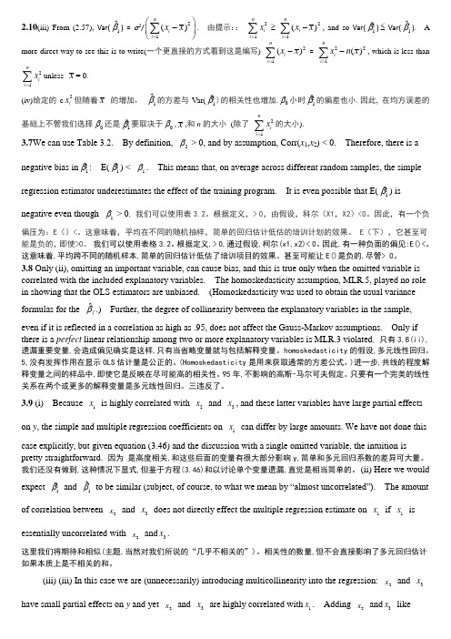
2.10(iii) From (2.57), Var(1ˆβ) = σ2/21()n i i x x =⎛⎫- ⎪⎝⎭∑. 由提示:: 21n ii x =∑ ≥ 21()n i i x x =-∑, and so Var(1β) ≤ Var(1ˆβ). A more direct way to see this is to write(一个更直接的方式看到这是编写) 21()ni i x x =-∑ = 221()n i i x n x =-∑, which is less than21n i i x=∑unless x = 0.(iv)给定的c 2i x 但随着x 的增加, 1ˆβ的方差与Var(1β)的相关性也增加.0β小时1β的偏差也小.因此, 在均方误差的基础上不管我们选择0β还是1β要取决于0β,x ,和n 的大小 (除了 21n i i x=∑的大小).3.7We can use Table 3.2. By definition, 2β > 0, and by assumption, Corr(x 1,x 2) < 0. Therefore, there is a negative bias in 1β: E(1β) < 1β. This means that, on average across different random samples, the simpleregression estimator underestimates the effect of the training program. It is even possible that E(1β) isnegative even though 1β > 0. 我们可以使用表3.2。
根据定义,> 0,由假设,科尔(X1,X2)<0。
因此,有一个负偏压为:E ()<。
这意味着,平均在不同的随机抽样,简单的回归估计低估的培训计划的效果。
伍德里奇 计量经济学导论

伍德里奇计量经济学导论摘要:一、引言1.计量经济学的基本概念2.计量经济学的研究方法与应用领域二、概率论与数理统计基础1.随机变量与概率分布2.数学期望与方差3.抽样分布与假设检验三、线性回归分析1.回归方程的建立与估计2.回归系数的显著性检验3.回归模型的诊断与修正四、多元线性回归分析1.多元线性回归模型的建立2.多元线性回归的求解方法3.多元线性回归的显著性检验五、时间序列分析1.时间序列的基本概念与特点2.平稳时间序列的判定与转换3.时间序列模型的建立与预测六、非参数统计方法1.非参数检验的基本思想与方法2.非参数回归与插值方法3.非参数统计方法的优缺点及应用场景七、计量经济学在实践中的应用1.我国经济发展中的计量经济学应用案例2.计量经济学在国际贸易、金融、环境等领域的应用3.计量经济学在政策评估与制定中的作用八、伍德里奇计量经济学导论的评价与启示1.教材的结构与内容特点2.伍德里奇计量经济学导论在我国的影响力3.对我国计量经济学教育的启示正文:计量经济学是一门运用概率论、统计学、数学等方法研究经济现象及其规律的科学。
在当今经济学领域,计量经济学已成为一门重要的分支学科,广泛应用于科研、教学和实践。
伍德里奇《计量经济学导论》一书,系统地阐述了计量经济学的基本原理、方法及应用,为读者提供了宝贵的理论指导和实践经验。
本书首先介绍了计量经济学的基本概念和研究方法。
计量经济学的研究方法主要包括实证分析、理论分析及实证与理论相结合的分析方法。
研究范围涉及宏观、微观及政策评估等多个领域。
此外,本书还简要介绍了概率论和数理统计的基本知识,为后续章节的学习奠定了基础。
在概率论和数理统计基础部分,本书详细讲解了随机变量、概率分布、数学期望、方差等概念,以及抽样分布、假设检验等统计方法。
这些知识为后续的回归分析提供了理论支持。
线性回归分析是计量经济学的重要内容之一。
本书介绍了回归方程的建立与估计、回归系数的显著性检验以及回归模型的诊断与修正方法。
伍德里奇 计量经济学导论

伍德里奇计量经济学导论摘要:I.引言A.计量经济学的重要性B.伍德里奇《计量经济学导论》的目的和适用对象II.计量经济学的概念与方法A.什么是计量经济学B.计量经济学的方法和工具III.经济模型与数据分析A.经济模型简介B.数据分析在计量经济学中的应用IV.最小二乘法A.最小二乘法的原理B.最小二乘法在回归分析中的应用V.回归分析A.回归模型的建立B.回归系数的估计与检验VI.模型的评估与选择A.模型评估的方法B.模型选择的原则VII.异方差性、序列相关性和其他问题A.异方差性的处理B.序列相关性的检验与处理C.其他可能出现的问题及解决方法VIII.实证分析与应用A.实证分析的步骤B.计量经济学在实际问题中的应用IX.总结与展望A.计量经济学导论的主要内容回顾B.计量经济学的发展趋势和前景正文:在当今经济学的各个领域中,计量经济学发挥着越来越重要的作用。
它不仅为经济理论提供了实证依据,而且为政策制定者提供了决策依据。
伍德里奇所著的《计量经济学导论》旨在为初学者提供一个关于计量经济学的全面认识,帮助他们掌握计量经济学的基本概念、方法和应用。
在本书中,伍德里奇首先介绍了计量经济学的重要性,以及本书的目的和适用对象。
接着,他对计量经济学的基本概念和方法进行了详细阐述,包括经济模型、数据分析、最小二乘法等。
此外,他还深入讲解了回归分析的原理和方法,以及如何对回归模型进行评估和选择。
在本书的后续章节中,伍德里奇对可能出现的问题,如异方差性、序列相关性等进行了讨论,并介绍了处理这些问题的方法。
他还通过实证分析,展示了计量经济学在实际问题中的应用,例如在通货膨胀、失业、贸易政策等方面的应用。
总之,《计量经济学导论》是一本很好的入门教材,它系统地介绍了计量经济学的基本概念、方法和应用。
计量经济学第三版-课后习题答案

计量经济学第三版-课后习题答案*************************************************************** ******************************************************************* ********************??第一章绪论(一)基本知识类题型1-1.什么是计量经济学?1-3.计量经济学方法与一般经济数学方法有什么区别?它在经济学科体系中的作用和地位是什么?1-6.计量经济学的研究的对象和内容是什么?计量经济学模型研究的经济关系有哪两个基本特征?1-7.试结合一个具体经济问题说明建立与应用计量经济学模型的主要步骤。
1-9.计量经济学模型主要有哪些应用领域?各自的原理是什么?1-12.模型的检验包括几个方面?其具体含义是什么?1-17.下列假想模型是否属于揭示因果关系的计量经济学模型?为什么?⑴ S t=112.0+0.12R t其中S t为第t年农村居民储蓄增加额(亿元)、R t为第t年城镇居民可支配收入总额(亿元)。
⑵ S t-1=4432.0+0.30R t其中S t-1为第(t-1)年底农村居民储蓄余额(亿元)、R t为第t年农村居民纯收入总额(亿元)。
1-18.指出下列假想模型中的错误,并说明理由:(1)RS t=8300.0-0.24RI t+112.IV t其中,RS t为第t年社会消费品零售总额(亿元),RI t为第t年居民收入总额(亿元)(城镇居民可支配收入总额与农村居民纯收入总额之和),IV t为第t年全社会固定资产投资总额1(亿元)。
(2)C t=180+1.2Y t其中,C、Y分别是城镇居民消费支出和可支配收入。
(3)ln Y t=1.15+1.62 ln K t-0.28ln L t其中,Y、K、L分别是工业总产值、工业生产资金和职工人数。
1-19.下列假想的计量经济模型是否合理,为什么?(1)GDP=α+∑βi GDP i+ε其中,GDP i(i=1,2,3)是第i产业的国内生产总值。
