机器学习中的优化算法综述

IPAM Summer School 2012
Tutorial on
Optimization methods for machine learning
Jorge Nocedal
Northwestern University
Overview 1. We discuss some characteristics of optimization problems arising in deep learning, convex logistic regression and inverse covariance estimation. 2. There are many tools at our disposal: first and second order methods; batch and stochastic algorithms; regularization; primal and dual approaches; parallel computing 3. Yet the state of affairs with neural nets is confusing to me: too many challenges are confronted at once: local vs local minima, nonlinearity, stochasticity, initializations, heuristics
pk = −rk + β k pk−1
p Ark βk = T pk −1 Apk −1
T k −1
Only product Apk is needed Hessian-free
Choose some initial point: x0 Initial direction: p0 = −r0 For x0 = 0, -r0 = b
6
Part I Problem Characteristics and Second Order Methods
7
Nonlinearity, Ill Conditioning Neural nets are far more nonlinear than the functions minimized in many other applications Farabet The rate of convergence of an optimization algorithm is still important even though in practice one stops the iteration far from a minimizer”
Problem: min f (x)
(Hessian Free)
∇ 2 f (xk )p = −∇f (xk ) xk +1 = xk + α p
- This is a linear system of equations of size n - Apply the Conjugate Gradient (CG) method to compute an approximate solution to this system - CG is an iterative method endowed with very interesting properties (optimal Krylov method) - Hessian need not be computed explicitly - Continuum between 1st and 2nd order methods
4
My Background Most of my practical experience in optimization methods for machine learning is for speech recognition (Google) But I am aware of many tests done in a variety of machine learning applications due to my involvement in L-BFGS, Newton-CG methods (Hessian-free), dynamic sampling methods, etc I am interested in designing new optimization methods for machine applications, in particular for deep learning
Interaction between CG and Newton
We noted -r = b if x0 = 0
For the linear system
∇ 2 f (xk )p = −∇f (xk ) Ax = b r = Ax −b → b = − ∇f (xk )
Conclusion: if we terminate the CG algorithm after 1 iteration we obtain a steepest descent step
3
Organization I will discuss a few of optimization techniques and provide some insights into their strengths and weaknesses We will contrast the deterministic and stochastic settings. This motivates dynamic sample selection methods We emphasize the need for general purpose techniques, second order methods and scale invariance, vs heuristics
The conjugate gradient method
Two equivalent problems
1 T min φ (x) = x Ax − bT x ∇φ (x) = Ax − b 2 solve Ax = b r = Ax − b
Newton-CG: the Convex Case
∇ 2 f (xk )p = −∇f (xk )
- We show below that any number of CG iterations yield a productive step - Not true of other iterative methods - better direction and length than 1st order methods
8
An objective function (Le,…Ng)
9
General Formulation
1 m min J (w) = ∑ (w;(zi , yi )) + ν || w ||1 m i =1
(z i , y i ) training data zi vector of features;
Difficult to choose γ . Trust region method learns γ
The Nonconvex Case: Alternatives
Replace ∇ 2 f (xk ) by a positive definite approximation Bp = −∇f (x0 ) Option 1: Gauss-Newton Matrix J(xk )J(xk )T Option 2: Stop CG early - negative curvature Option 3: Trust region approach
1
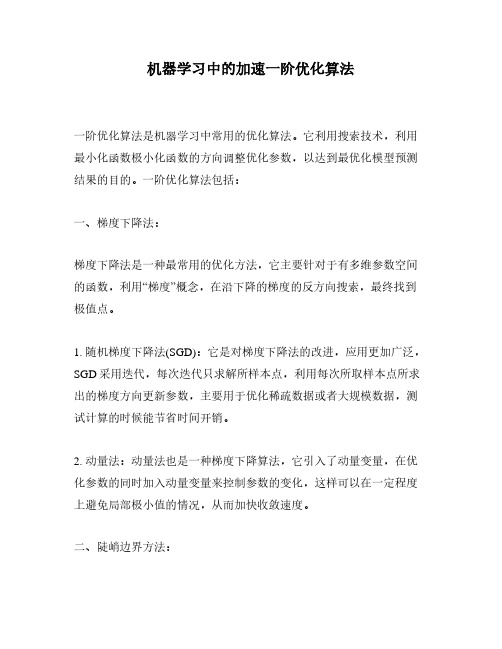
n Newton
Steepest descent
Rates of Convergence – Scale Invariance
The rate of convergence can be: linear superlinear quadratic depending on the accuracy of the CG solution • It inherits some of the scale invariance properties of the exact Newton method: affine change of variables x ← Dx
Let λ1 ≤ λ2 ≤ ... ≤ λn be the eigenvalues of ∇ 2 f (x0 ). Then the eigenvalues of [∇ 2 f (x0 ) + γ I ] are: λ1 + γ ≤ λ2 + γ ≤ ... ≤ λn + γ
Newton-CG Framework
Theorem (Newton-CG with any number of CG steps) Suppose that f is strictly convex. Consider the iteration ∇ 2 f (xk )p = −∇f (xk ) + r xk +1 = xk + α p where α is chosen by a backtracking Armijo line search. Then {xk } → x*
2
Open Questions We need to isolate questions related to optimization, and study them in a controlled setting A key question is to understand the properties of stochastic vs batch methods in the context of deep learning. After some clarity is obtained, we need to develop appropriate algorithms and work complexity bounds, both in a sequential and a parallel setting