Ansys 共轭传热分析实例
ANSYS传热分析实例汇总
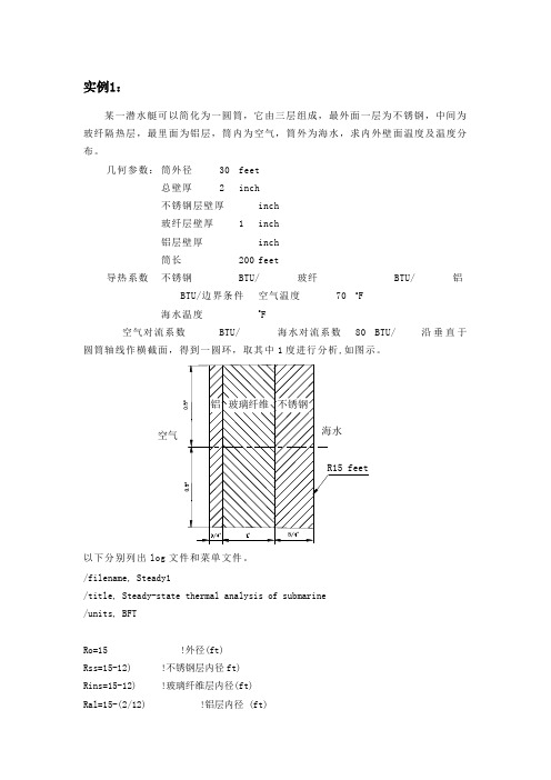
实例1:某一潜水艇可以简化为一圆筒,它由三层组成,最外面一层为不锈钢,中间为玻纤隔热层,最里面为铝层,筒内为空气,筒外为海水,求内外壁面温度及温度分布。
几何参数:筒外径30 feet总壁厚 2 inch不锈钢层壁厚inch玻纤层壁厚 1 inch铝层壁厚inch筒长200 feet导热系数不锈钢BTU/ 玻纤BTU/ 铝BTU/边界条件空气温度70 o F海水温度o F空气对流系数BTU/ 海水对流系数80 BTU/沿垂直于圆筒轴线作横截面,得到一圆环,取其中1度进行分析,如图示。
以下分别列出log文件和菜单文件。
/filename, Steady1/title, Steady-state thermal analysis of submarine/units, BFTRo=15 !外径(ft)Rss=15-12) !不锈钢层内径ft)Rins=15-12) !玻璃纤维层内径(ft)Ral=15-(2/12) !铝层内径 (ft)Tair=70 !潜水艇内空气温度Tsea= !海水温度Kss= !不锈钢的导热系数 (BTU/ !玻璃纤维的导热系数 (BTU/ !铝的导热系数(BTU/ !空气的对流系数(BTU/ !海水的对流系数(BTU/ !定义二维热单元mp,kxx,1,Kss !设定不锈钢的导热系数mp,kxx,2,Kins !设定玻璃纤维的导热系数mp,kxx,3,Kal !设定铝的导热系数pcirc,Ro,Rss,, !创建几何模型pcirc,Rss,Rins,,pcirc,Rins,Ral,,aglue,allnumcmp,arealesize,1,,,16 !设定划分网格密度lesize,4,,,4lesize,14,,,5lesize,16,,,2eshape,2 !设定为映射网格划分mat,1amesh,1mat,2amesh,2mat,3amesh,3/SOLUSFL,11,CONV,HAIR,,TAIR !施加空气对流边界SFL,1,CONV,HSEA,,TSEA !施加海水对流边界SOLVE/POST1PLNSOL !输出温度彩色云图finish菜单操作:1.U tility Menu>File>change jobename, 输入Steady1;2.U tility Menu>File>change title,输入Steady-state thermal analysis ofsubmarine;3.在命令行输入:/units, BFT;4.M ain Menu: Preprocessor;5.M ain Menu: Preprocessor>Element Type>Add/Edit/Delete,选择PLANE55;6.M ain Menu: Preprocessor>Material Prop>-Constant-Isotropic,默认材料编号为1,在KXX框中输入,选择APPLY,输入材料编号为2,在KXX框中输入,选择APPLY,输入材料编号为3,在KXX框中输入;7.M ain Menu: Preprocessor>-Modeling->Create>-Areas-Circle>By Dimensions ,在RAD1中输入15,在RAD2中输入15-(.75/12),在THERA1中输入,在THERA2中输入,选择APPLY,在RAD1中输入15-(.75/12),在RAD2中输入15-12),选择APPLY,在RAD1中输入15-12),在RAD2中输入15-2/12,选择OK;8.M ain Menu: Preprocessor>-Modeling->Operate>-Booleane->Glue>Area,选择PICK ALL;9.M ain Menu: Preprocessor>-Meshing-Size Contrls>-Lines-Picked Lines,选择不锈钢层短边,在NDIV框中输入4,选择APPLY,选择玻璃纤维层的短边,在NDIV框中输入5,选择APPLY,选择铝层的短边,在NDIV框中输入2,选择APPLY,选择四个长边,在NDIV中输入16;10.Main Menu: Preprocessor>-Attributes-Define>Picked Area,选择不锈钢层,在MAT框中输入1,选择APPLY,选择玻璃纤维层,在MAT框中输入2,选择APPLY,选择铝层,在MAT 框中输入3,选择OK;11.Main Menu: Preprocessor>-Meshing-Mesh>-Areas-Mapped>3 or 4 sided,选择PICKALL;12.Main Menu: Solution>-Loads-Apply>-Thermal-Convection>On lines,选择不锈钢外壁,在VALI框中输入80,在VAL2I框中输入,选择APPLY,选择铝层内壁,在VALI框中输入,在VAL2I框中输入70,选择OK;13.Main Menu: Solution>-Solve-Current LS;14.Main Menu: General Postproc>Plot Results>-Contour Plot-Nodal Solu,选择Temperature。
ANSYS-热分析(两个实例)有限元热分析上机指导书
第四讲 热分析上机指导书CAD/CAM 实验室,USTC实验要求:1、通过对冷却栅管的热分析练习,熟悉用ANSYS 进行稳态热分析的基本过程,熟悉用直接耦合法、间接耦合法进行热应力分析的基本过程。
2、通过对铜块和铁块的水冷分析,熟悉用ANSYS 进行瞬态热分析的基本过程。
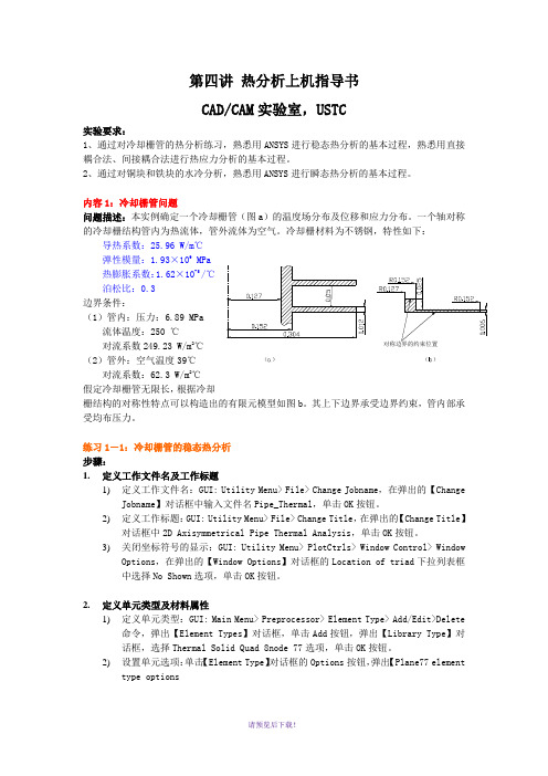
内容1:冷却栅管问题问题描述:本实例确定一个冷却栅管(图a )的温度场分布及位移和应力分布。
一个轴对称的冷却栅结构管内为热流体,管外流体为空气。
冷却栅材料为不锈钢,特性如下:导热系数:25.96 W/m ℃弹性模量:1.93×10⁹ MPa热膨胀系数:1.62×10⁻⁵ /℃泊松比:0.3边界条件:(1)管内:压力:6.89 MPa流体温度:250 ℃对流系数249.23 W/m 2℃(2)管外:空气温度39℃对流系数:62.3 W/m 2℃假定冷却栅管无限长,根据冷却栅结构的对称性特点可以构造出的有限元模型如图b 。
其上下边界承受边界约束,管内部承受均布压力。
练习1-1:冷却栅管的稳态热分析步骤:1. 定义工作文件名及工作标题1) 定义工作文件名:GUI: Utility Menu> File> Change Jobname ,在弹出的【ChangeJobname 】对话框中输入文件名Pipe_Thermal ,单击OK 按钮。
2) 定义工作标题:GUI: Utility Menu> File> Change Title ,在弹出的【Change Title 】对话框中2D Axisymmetrical Pipe Thermal Analysis ,单击OK 按钮。
3) 关闭坐标符号的显示:GUI: Utility Menu> PlotCtrls> Window Control> WindowOptions ,在弹出的【Window Options 】对话框的Location of triad 下拉列表框中选择No Shown 选项,单击OK 按钮。
ANSYS温度场例题分析
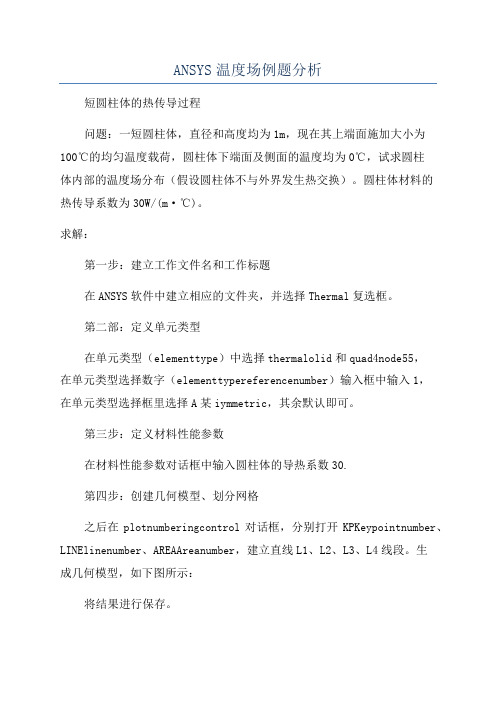
ANSYS温度场例题分析短圆柱体的热传导过程问题:一短圆柱体,直径和高度均为1m,现在其上端面施加大小为100℃的均匀温度载荷,圆柱体下端面及侧面的温度均为0℃,试求圆柱体内部的温度场分布(假设圆柱体不与外界发生热交换)。
圆柱体材料的热传导系数为30W/(m·℃)。
求解:第一步:建立工作文件名和工作标题在ANSYS软件中建立相应的文件夹,并选择Thermal复选框。
第二部:定义单元类型在单元类型(elementtype)中选择thermalolid和quad4node55,在单元类型选择数字(elementtypereferencenumber)输入框中输入1,在单元类型选择框里选择A某iymmetric,其余默认即可。
第三步:定义材料性能参数在材料性能参数对话框中输入圆柱体的导热系数30.第四步:创建几何模型、划分网格之后在plotnumberingcontrol对话框,分别打开KPKeypointnumber、LINElinenumber、AREAAreanumber,建立直线L1、L2、L3、L4线段。
生成几何模型,如下图所示:将结果进行保存。
第五步:加载求解选择分析类型Steady-State,在SelectEntitie对话框,第一个下拉列表框中选择Line,在第二个下拉列表中选择ByNum,第三个单选框中选择FromFull。
选择线段L1、L2。
重复上述操作,在SelectEntitie对话框,第一个下拉列表框中选择Node,在第二个下拉列表中选择Attachedto,第三个单选框中选择Line,all。
并在Lab2DOFtobecontrained列表中选择TEMP,在VALUELoadTEMPvalue输入框中输入0。
在SelectEntitie对话框,第一个下拉列表框中选择Line,在第二个下拉列表中选择ByNum,第三个单选框中选择FromFull选择L3线段,重复上述操作,在SelectEntitie对话框,第一个下拉列表框中选择Node,在第二个下拉列表中选择Attachedto,第三个单选框中选择Line,all。
ANSYS流体与热分析第10章热分析典型工程实例

第10 章热分析典型工程实例本章要点拉伸特征旋转特征扫掠特征混合特征孔特征壳特征本章案例某型号手机电池的散热分析冷库复合隔热板热量流动分析电子元器件散热装置温度分析10.1 工程实例1——某型号手机电池的散热分析该算例为某型手机电池的散热分析,如图10-1为某型号手机背面的照片,图中可见手机的电池的位置。
在手机工作时,电池可向外传递热量。
使用手机的读者应该都体会过手机电池发热的现象,特别是在长时间接打电话时,这种现象尤为明显。
本实例对某型号手机进行分析,电池的标准电压为3.7V,电池容量为750mAh。
试求手机开机状态下外壳的温度分布。
手机的各部分材料性能参数如表10.1所示。
图10-1 手机背面照片在计算分析过程中我们将手机看做三个组成部分:塑料外壳、手机内部材料和手机电池。
忽略手机内部线路和芯片,可以将手机电池看做唯一热源。
简化后的手机模型如图10-2所示,图中单位均为cm。
本实例拟采用Solid Tet 10node 87单元进行分析。
由于电池功率和环境温度均可视为恒定不变,因此分析类型为稳态。
图10-2 简化后的手机模型由电池的电压和电流可以算得电池的功率:==⨯=P UI 3.70.75 2.775W电池的体积为:3=⨯⨯=V0.040.010.050.00002m电池的发热量:3==Q P/V138750W/m——附带光盘“Ch10\实例10-1_start”——附带光盘“Ch10\实例10-1_end”——附带光盘“A VI\Ch10\10-1.avi”1、定义分析文件名1、选择Utility Menu>File>Change Jobname,在弹出的单元增添对话框中输入Example10-1,然后点击OK按钮。
2、选择Main Menu>Preferences,弹出Preferences for GUI Filtering对话框,点选Thermal复选框,单击OK按钮关闭该对话框。
ANSYS Workbench热力学分析实例演练(2020版

第7章非线性热分析
7.1非线性热分析概述 7.2平板非线性热分析 7.3本章小结
第8章热辐射分析
8.1基本概念 8.2空心半球与平板的热辐射分析 8.3本章小结
第9章相变分析
第10章优化分 析
第11章热应力 耦合分析
第12章热流耦 合分析
第9章相变分析
9.1相变分析简介 9.2飞轮铸造相变模拟分析 9.3本章小结
作者介绍
同名作者介绍
这是《ANSYS Workbench热力学分析实例演练(2020版)》的读书笔记模板,暂无该书作者的介绍。
读书笔记
读书笔记
这是《ANSYS Workbench热力学分析实例演练(2020版)》的读书笔记模板,可以替换为自己的心得。
精彩摘录
精彩摘录
这是《ANSYS Workbench热力学分析实例演练(2020版)》的读书笔记模板,可以替换为自己的精彩内容摘 录。
第10章优化分析
10.1优化分析简介 10.2散热肋片优化分析 10.3本章小结
第11章热应力耦合分析
11.1热应力概述 11.2瞬态热应力分析 11.3热应力对结构模态的影响分析 11.4热疲劳分析 11.5本章小结
第12章热流耦合分析
12.1 CFX流场分析 12.2 Fluent流场分析 12.3 Icepak流场分析 12.4本章小结
ANSYS Workbench热力学分析 实例演练(2020版
读书笔记模板
01 思维导图
03 目录分析 05 读书笔记
目录
02 Байду номын сангаас容摘要 04 作者介绍 06 精彩摘录
思维导图
本书关键字分析思维导图
工程
实例
ansys热分析实例教程
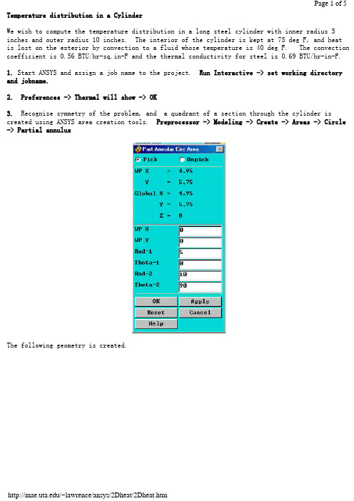
Temperature distribution in a CylinderWe wish to compute the temperature distribution in a long steel cylinder with inner radius 5 inches and outer radius 10 inches. The interior of the cylinder is kept at 75 deg F, and heatis lost on the exterior by convection to a fluid whose temperature is 40 deg F. The convection coefficient is 0.56 BTU/hr-sq.in-F and the thermal conductivity for steel is 0.69 BTU/hr-in-F.1. Start ANSYS and assign a job name to the project. Run Interactive -> set working directory and jobname.2. Preferences -> Thermal will show -> OK3. Recognize symmetry of the problem, and a quadrant of a section through the cylinder is created using ANSYS area creation tools. Preprocessor -> Modeling -> Create -> Areas -> Circle -> Partial annulusThe following geometry is created.4. Preprocessor -> Element Type -> Add/Edit/Delete -> Add -> Thermal Solid -> Solid 8 node 77 -> OK -> Close5. Preprocessor -> Material Props -> Isotropic -> Material Number 1 -> OKEX = 3.E7 (psi)DENS = 7.36E-4 (lb sec^2/in^4)ALPHAX = 6.5E-6PRXY = 0.3KXX = 0.69 (BTU/hr-in-F)6. Mesh the area and refine using methods discussed in previous examples.7. Preprocessor -> Loads -> Apply -> Temperatures -> NodesSelect the nodes on the interior and set the temperature to 75.8. Preprocessor -> Loads -> Apply -> Convection -> LinesSelect the lines defining the outer surface and set the convection coefficient to 0.56 and the fluid temp to 40.9. Preprocessor -> Loads -> Apply -> Heat Flux -> LinesTo account for symmetry, select the vertical and horizontal lines of symmetry and set the heat flux to zero.10. Solution -> Solve current LS11. General Postprocessor -> Plot Results -> Nodal Solution -> TemperaturesThe temperature on the interior is 75 F and on the outside wall it is found to be 45. These results can be checked using results from heat transfer theory.BackThermal Stress of a Cylinder using Axisymmetric ElementsA steel cylinder with inner radius 5 inches and outer radius 10 inches is 40 inches long and has spherical end caps. The interior of the cylinder is kept at 75 deg F, and heat is lost on the exterior by convection to a fluid whose temperature is 40 deg F. The convection coefficient is 0.56 BTU/hr-sq.in-F. Calculate the stresses in the cylinder caused by the temperature distribution.The problem is solved in two steps. First, the geometry is created, the preference set to'thermal', and the heat transfer problem is modeled and solved. The results of the heat transfer analysis are saved in a file 'jobname.RTH' (Results THermal analysis) when you issue a save jobname.db command.Next the heat transfer boundary conditions and loads are removed from the mesh, the preference is changed to 'structural', the element type is changed from 'thermal' to 'structural', and the temperatures saved in 'jobname.RTH' are recalled and applied as loads.1. Start ANSYS and assign a job name to the project. Run Interactive -> set working directory and jobname.2. Preferences -> Thermal will show -> OK3. A quadrant of a section through the cylinder is created using ANSYS area creation tools.4. Preprocessor -> Element Type -> Add/Edit/Delete -> Add -> Solid 8 node 77 -> OK ->Options -> K3 Axisymmetric -> OK5. Preprocessor -> Material Props -> Isotropic -> Material Number 1 -> OKEX = 3.E7 (psi)DENS = 7.36E-4 (lb sec^2/in^4)ALPHAX = 6.5E-6PRXY = 0.3KXX = 0.69 (BTU/hr-in-F)6. Mesh the area using methods discussed in previous examples.7. Preprocessor -> Loads -> Apply -> Temperatures -> NodesSelect the nodes on the interior and set the temperature to 75.8. Preprocessor -> Loads -> Apply -> Convection -> LinesSelect the lines defining the outer surface and set the coefficient to 0.56 and the fluid temp to 40.9. Preprocessor -> Loads -> Apply -> Heat Flux -> LinesSelect the vertical and horizontal lines of symmetry and set the heat flux to zero.10. Solution -> Solve current LS11. General Postprocessor -> Plot Results -> Nodal Solution -> TemperatureThe temperature on the interior is 75 F and on the outside wall it is found to be 43.12. File -> Save Jobname.db13. Preprocessor -> Loads -> Delete -> Delete All -> Delete All Opts.14. Preferences -> Structural will show, Thermal will NOT show.15. Preprocessor -> Element Type -> Switch Element Type -> OK (This changes the element to structural)16. Preprocessor -> Loads -> Apply -> Displacements -> Nodes(Fix nodes on vertical and horizontal lines of symmetry from crossing the lines of symmetry.)17. Preprocessor -> Loads -> Apply -> Temperature -> From Thermal AnalysisSelect Jobname.RTH (If it isn't present, look for the default 'file.RTH' in the root directory)18. Solution -> Solve Current LS19. General Postprocessor -> Plot Results -> Element Solution - von Mises StressThe von Mises stress is seen to be a maximum in the end cap on the interior of the cylinder and would govern a yield-based design decision.Back。
ansys基本热传递分析

Workshop 1
基本热传递分析
问题描述: 问题描述 • 长矩形板在上下表面受热对流
分析目的: 分析目的 • 对板做2-D热分析并用手工计算 热分析并用手工计算 对板做 校核。 校核。
详细描述见下。根据箭头指示 详细描述见下。 选取菜单项。 选取菜单项。
本例的ANSYS命令流文件在附录 C中。 命令流文件在附录 中 本例的
步骤 6: 续…定义板的几何模型 定义板的几何模型
1 2
注: 坐标相对于工作平面坐标系,缺省在全局 坐标相对于工作平面坐标系, 坐标系原点。 坐标系原点。
3
菜单拾取
步骤 6: 续……显示线段。 显示线段。 显示线段
1
look
菜单拾取
指定缺省(全局 全局)属性 步骤 7: 指定缺省 全局 属性
2
1 3
1
4
2 3 查看此信息
菜单拾取
现在, 步骤 16: 续…现在,将温度结果映射到路径上,并给它一个标记 现在 将温度结果映射到路径上, “tupper”。 。
1
2
注: 不影响 DOF项。
3
菜单拾取
步骤 16: 续…选择 绘制“tupper”项 选择 绘制“ 项
1
2 3
菜单拾取
look
菜单拾取
步骤 17: 列出 “tupper”路径的结果 路径的结果
注: 缺省单元属性与单元厚度共面。 缺省单元属性与单元厚度共面。 虽然在本题中不需要,但如果单元 虽然在本题中不需要, 是轴对称的,请改动。 是轴对称的,请改动。
1
菜单拾取
输入材料特性。 步骤 5: 输入材料特性。
1 3
2
4
5
步骤 6: 生成板 的几何模型。 的几何模型。
Ansys共轭传热分析实例
共轭传热计算(2012-12-19 09:53:07)转载▼标签:杂谈分类:FLUENT技巧共轭传热:流体传热与固体传热相互耦合。
由于流体求解器同时具备流体与固体传热计算的能力,因此可以直接采用流体求解器进行求解,无需使用流固耦合计算。
流体求解器能够求解流体对流、传导、辐射传热,对于固体传热计算,只能求解热传导方程。
本例演示共轭传热问题在FLUENT中的求解方法。
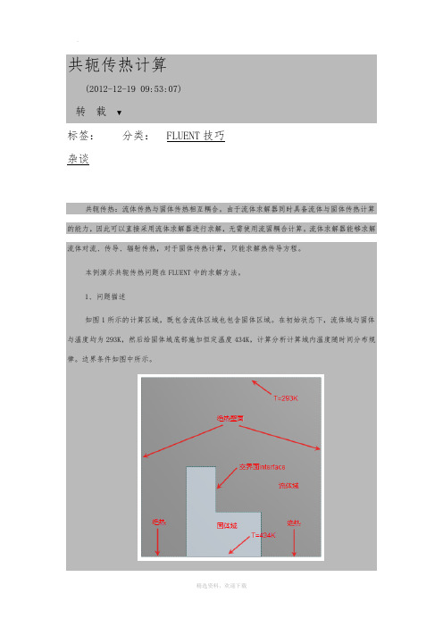
1、问题描述如图1所示的计算区域,既包含流体区域也包含固体区域。
在初始状态下,流体域与固体与温度均为293K,然后给固体域底部施加恒定温度434K,计算分析计算域内温度随时间分布规律。
边界条件如图中所示。
图1 计算域描述2、建立几何模型并划分网格利用DM建立如图1所示2D平面几何。
采用全四边形网格划分,如图2所示。
为所有边界命名,尤其是流体和固体区域交界面,后面需要在求解器中进行设置。
3、进入Fluent求解设置本例为瞬态计算。
涉及到热量传递,因此需要激活能量方程。
流体介质为理想气体,考虑其在温度影响下密度变化。
考虑重力影响,设置重力加速度向量[0,-9.81,0],设置操作密度为0。
如图3所示。
压力-速度耦合方程采用PISO求解方式,对流项计算采用QUICK算法,其他项采用二阶迎风格式。
图2 网格模型图3 操作项设置面板设置流体域介质为air,固体域介质为默认的AL。
按图1所示边界条件设置计算域边界。
创建交界面,如图4所示进行设置。
图4 设置交界面4、初始化计算设置初始化温度293K,如图5所示。
图5 初始化面板设置自动保存选项与动画录制项。
设置时间步长0.1s,时间步数100,内迭代次数20基于Fluent与ANSYS workbench的齿轮箱热固耦合温度场仿真案例2015-12-08 17:45:383966简介:今天为大家带来齿轮箱瞬态温度场仿真的原创案例。
限于篇幅,这个帖子不像之前一样把所有设置一步步贴图,因此只给出关键图,设置全部给出了表格形式。
ANSYS Fluent 在热分析中的使用介绍
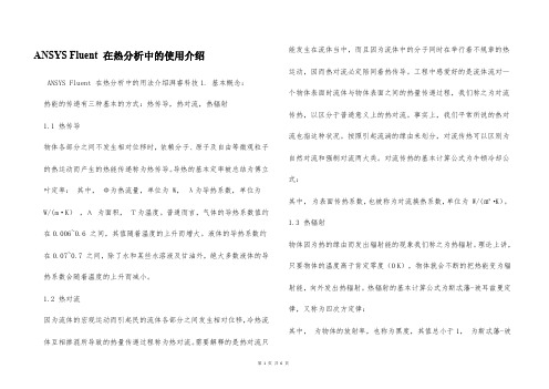
ANSYS Fluent 在热分析中的使用介绍ANSYS Fluent 在热分析中的用法介绍湃睿科技1. 基本概念:热能的传递有三种基本的方式:热传导,热对流,热辐射1.1 热传导物体各部分之间不发生相对位移时,依赖分子、原子及自由等微观粒子的热运动而产生的热能传递称为热传导。
导热的基本定率被总结为傅立叶定率:其中,Φ为热流量,单位为 W,λ为导热系数,单位为W/(m·K),Α为面积,Τ为温度。
普通而言,气体的导热系数值约在0.006~0.6 之间,其值随着温度的上升而增大。
液体的导热系数约在0.07~0.7 之间,除了水和某些水溶液及甘油外,绝大多数液体的导热系数会随着温度的上升而减小。
1.2 热对流因为流体的宏观运动而引起民的流体各部分之间发生相对位移,冷热流体互相掺混所导致的热量传递过程称为热对流。
需要解释的是热对流只能发生在流体当中,而且因为流体中的分子同时在举行着不规章的热运动,因而热对流必定陪同着热传导。
工程中感爱好的是流体流对一个物体表面时流体与物体表面之间的热量传递过程,我们称之为对流传热,以区分于普通意义上的热对流。
事实上,我们平常所说的热对流也指这种状况。
按照引起流淌的缘由来划分,对流传热可以区别为自然对流和强制对流两大类。
对流传热的基本计算公式为牛顿冷却公式:其中,为表面传热系数,也被称为对流换热系数,单位为 W/(㎡·K)。
1.3 热辐射物体因为热的缘由而发出辐射能的现象我们称之为热辐射。
理论上讲,只要物体的温度高于肯定零度(0 K),物体就会不断的把热能变为辐射能,向外发出热辐射。
热辐射的基本计算公式为斯忒藩-玻耳兹曼定律,又称为四次方定律:其中,为物体的放射率,也称为黑度,其值总小于1,为斯忒藩-玻耳兹曼常量,它是个自然常数,其值为5.67e-08W/(㎡·K4), T为热力学温度,单位 K。
以上为三种基本传热方式的介绍,在实际问题中,这些方式往往不是单独浮现的,很可能是多种传热方式的组合形式。
ansys热分析例题

(瞬态)a n s y s热分析例题2(总5页)--本页仅作为文档封面,使用时请直接删除即可----内页可以根据需求调整合适字体及大小--问题描述:一个30公斤重、温度为70℃的铜块,以及一个20公斤重、温度为80℃的铁块,突然放入温度为20℃、盛满了300升水的、完全绝热的水箱中,如图所示。
过了一个小时,求铜块与铁块的最高温度(假设忽略水的流动)。
材料热物理性能如下:热性能单位制铜铁水导热系数W/m℃ 383 37密度Kg/m 8889 7833 996比热J/kg℃ 390 448 4185菜单操作过程:一、设置分析标题1、选择“Utility Menu>File>Change Jobname”,输入文件名Transient1。
2、选择“Utility Menu>File>Change Title”输入Thermal Transient Exercise 1。
二、定义单元类型1、选择“Main Menu>Preprocessor”,进入前处理。
2、选择“Main Menu>Preprocesor>Element Type>Add/Edit/Delete”。
选择热平面单元plane77。
三、定义材料属性1、选择“Main Menu>Preprocessor>Material Props>Material Models”,在弹出的材料定义窗口中顺序双击Thermal选项。
2、点击Conductivity,Isotropic,在KXX框中输入383;点击Density,在DENS框中输入8898;点击Specific Heat,在C框中输入390。
3、在材料定义窗口中选择Material>New Model,定义第二种材料。
4、点击Conductivity,Isotropic,在KXX框中输入70;点击Density,在DENS框中输入7833;点击Specific Heat,在C框中输入448。
ANSYS Example07热-结构耦合分析算例 (ANSYS)

k,4,8,
k,0,6
k,5,0,8
larc,2,3,1,5
larc,4,5,1,8
l,2,4
l,3,5
al,1,2,3,4
esize,0.5
amesh,all
!!!!!!!!!!!!!
FINISH
/SOL
!*
ANTYPE,0
DL,1, ,TEMP,1000,0
DL,2, ,TEMP,20,0
(6)下面首先进入热分析,进入ANSYS主菜单Solution->Analysis Type->New Analysis,设置分析类型为稳态分析Steady-state
(7)输入热边界条件,进入ANSYS主菜单Solution-> Define Loads-> Apply-> Thermal-> Temperature-> On Lines,在直线1上加上1000度的温度荷载,如图所示,在直线2上加上20度的温度荷载。
(5)下面划分网格,由于本模型只有一种单元一种材料,所以不必复杂的设置属性。进入ANSYS主菜单Preprocessor->Meshing->Size Cntrls->ManualSize->Global->Size,在Global Element Size窗口中设置单元尺寸为0.5。在ANSYS主菜单Preprocessor->Meshing->Mesh->Areas,点选圆环进行网格划分
solve
!!!!!!!!!!!!
FINISH
/POST1
!*
/EFACET,1
PLNSOL, TEMP,, 0
FINISH
Ansys培训5WB_DS作业1-泵室传热特性分析(精)

Training Manual
ANSYS Workbench - DesignMo 后处理
Training Manual
• 现在可以显示两个模型的外表面温度分布状况的图象,注意:正 如前面显示的图象那样,这些云图的显示不会受内部温度的影响
Polyethylene Aluminum
Training Manual
ANSYS Workbench - DesignModeler
13
14 15
作业6-求解
• 添加温度和总热流结果 16. 点击 Solution 分支. 17. “RMB > Insert > Thermal > Temperature”
16
Training Manual
ANSYS Workbench - DesignModeler
作业6 – 报告
Training Manual
ANSYS Workbench - DesignModeler
• 如果时间允许的话,可以抓取一些图片,放在报告中,并产生这 些报告
Training Manual
泵室传热特性分析
作业6 -目的
Training Manual
ANSYS Workbench - DesignModeler
• 在这个练习中,我们将分析泵壳(如下图示)的传热特性 • 在相同边界条件下,分别定义一个塑料制泵壳和一个铝制泵壳进行 分析 • 我们的目的是比较各种结构外露表面的温度并研究热流的分布
ANSYS Workbench - DesignModeler
17
•
重复上述步骤,添加 “Total Heat Flux”.
作业6-复制模型
• 在求解之前,我们要复制模 型,并定义另一种材料, 这 样我们才能比较两者之间的 区别 18. 点击 “Model” 分支. 19. “RMB > Duplicate”. 20. 在新分支的 “Model2” 中点 击 “Part1” 21. 在detail 窗口, 选材料为 “Aluminum”.
四个ANSYS热分析经典例子
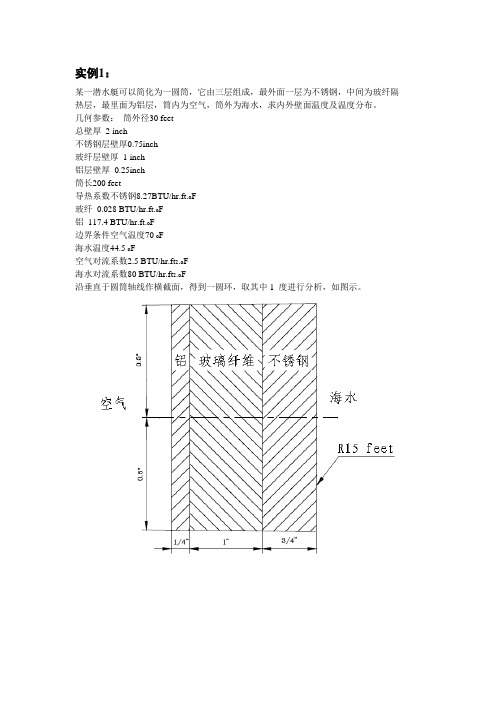
实例1:某一潜水艇可以简化为一圆筒,它由三层组成,最外面一层为不锈钢,中间为玻纤隔热层,最里面为铝层,筒内为空气,筒外为海水,求内外壁面温度及温度分布。
几何参数:筒外径30 feet总壁厚2 inch不锈钢层壁厚0.75inch玻纤层壁厚1 inch铝层壁厚0.25inch筒长200 feet导热系数不锈钢8.27BTU/hr.ft.o F玻纤0.028 BTU/hr.ft.o F铝117.4 BTU/hr.ft.o F边界条件空气温度70 o F海水温度44.5 o F空气对流系数2.5 BTU/hr.ft2.o F海水对流系数80 BTU/hr.ft2.o F沿垂直于圆筒轴线作横截面,得到一圆环,取其中1 度进行分析,如图示。
/filename,Steady1/title,Steady-state thermal analysis of submarine/units,BFTRo=15 !外径(ft)Rss=15-(0.75/12) !不锈钢层内径ft)Rins=15-(1.75/12) !玻璃纤维层内径(ft)Ral=15-(2/12) !铝层内径(ft)Tair=70 !潜水艇内空气温度Tsea=44.5 !海水温度Kss=8.27 !不锈钢的导热系数(BTU/hr.ft.oF)Kins=0.028 !玻璃纤维的导热系数(BTU/hr.ft.oF)Kal=117.4 !铝的导热系数(BTU/hr.ft.oF)Hair=2.5 !空气的对流系数(BTU/hr.ft2.oF)Hsea=80 !海水的对流系数(BTU/hr.ft2.oF)prep7et,1,plane55 !定义二维热单元mp,kxx,1,Kss !设定不锈钢的导热系数mp,kxx,2,Kins !设定玻璃纤维的导热系数mp,kxx,3,Kal !设定铝的导热系数pcirc,Ro,Rss,-0.5,0.5 !创建几何模型pcirc,Rss,Rins,-0.5,0.5pcirc,Rins,Ral,-0.5,0.5aglue,allnumcmp,arealesize,1,,,16 !设定划分网格密度lesize,4,,,4lesize,14,,,5lesize,16,,,2Mshape,2 !设定为映射网格划分mat,1amesh,1mat,2amesh,2mat,3amesh,3/SOLUSFL,11,CONV,HAIR,,TAIR !施加空气对流边界SFL,1,CONV,HSEA,,TSEA !施加海水对流边界SOLVE/POST1PLNSOL !输出温度彩色云图finish实例2一圆筒形的罐有一接管,罐外径为3 英尺,壁厚为0.2 英尺,接管外径为0.5 英尺,壁厚为0.1英尺,罐与接管的轴线垂直且接管远离罐的端部。
Ansys 热分析实例(多芯片组件加散热器(热沉)的冷却分析)
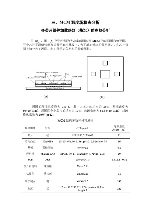
三.MCM温度场稳态分析多芯片组件加散热器(热沉)的冷却分析图1(a) 、图1(b) 所示分别为大功率球栅阵列MCM的截面图和俯视图,五个芯片采用倒装焊方式置于有机基板上,为了增加模块的散热能力,在芯片背面上加一热扩展面。
表1所示为各材料的物理属性。
周围的环境温度设为250 o C,其中大芯片的功率为25W,热流密度为60×106W/m3;周围四个小芯片的功率为10W,热流密度为61.54×106W/m3;对流换热系数为10W/(m·K)。
MCM结构参数和材料属性模型组件材料尺寸(mm)导热系数(W/(m﹒k))芯片硅8*8*0.65,5*5*0.65 82芯片凸点5Sn/98Pb 10*10*,6*6,Ø0.3,Height:0.2,Pitch:0.7536 基板聚酰亚胺40*40*1.5 0.2焊料球96.5Sn3.5Ag 26*26,Ø0.6, Height:0.4,Pitch:1.2750PCB FR4 100*100*1.5 8.37,8.37,0.32 热介质材料导热脂Thick:0.15 1粘接剂粘接剂Thick:0.15 1.1热扩展面铜40*40*1.5 390热沉铝Base:46.5*45.6*1.5,Pin number:16,Pinheight:8240分析从而导致器件性能变化和可靠性的下降。
热场分析和设计是MCM设计中一个重要的环节[3]。
MCM器件中的热应力来自两个方面,即来自MCM模块内部和MCM模块所处的外部环境所形成的热应力,这些热应力都会影响到器件的电性能、工作频率、机械强度和可靠性。
随着MCM集成度的提高和体积的缩小,尤其是对于集成了大功率芯片的MCM ,其内部具有多个热源,热源之间的热耦合作用较强,单位体积内的功耗很大,由此带来的芯片热失效和热退化现象突出。
有资料表明,器件的工作温度每升高10o C,其失效率增加1倍[4]。
带有共轭换热的流动
CFX 10.0
© 2005 ANSYS, Inc.
October 11, 2005 Inventory #002279
P3-9
边界条件(Boundary Conditions)
定义入口边界条件,名字=inlet,位置=inlet,流体法向速度=0.8 [m/s],静温=300 [K],默认湍流值 定义出口边界条件,名字=outlet,位置=outlet,平均静压=0 [Pa] 定义对称边界条件,名字=symm,位置=symmet 定义壁面边界条件:
CFX 10.0
© 2005 ANSYS, Inc.
October 11, 2005 Inventory #002279
P3-5
定义流体域(Define Fluid Domain)
CFX 10.0
© 2005 ANSYS, Inc.
October 11, 2005 Inventory #002279
P3-6
定义固体域(Define Solid Domains)
在CFX-Pre工作区单击Physics标签 在主工具条中单击Domain 命名为solidfin1 ,然后单击OK 在 General Options面板: - 设置Location为Assembly - 设置Domain Type为Solid Domain - 设置Solids List为Steel 在Domain Models中: - 设置Domain Motion为Stationary 在Solid Models面板: - 在Heat Transfer Model中,设置Option=Thermal Energy - 对于Thermal Radiation Model,保持Option=None
4.CFX共轭传热实例
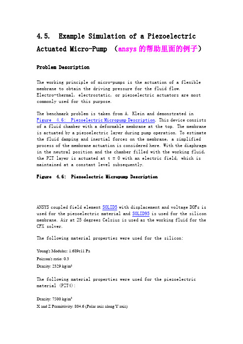
4.5. Example Simulation of a Piezoelectric Actuated Micro-Pump (ansys的帮助里面的例子)Problem DescriptionThe working principle of micro-pumps is the actuation of a flexible membrane to obtain the driving pressure for the fluid flow.Electro-thermal, electrostatic, or piezoelectric actuators are most commonly used for this purpose.The benchmark problem is taken from A. Klein and demonstrated in Figure 4.6: Piezoelectric Micropump Description. This device consists of a fluid chamber with a deformable membrane at the top. The membrane is actuated by a piezoelectric layer during pump operation. To estimate the fluid damping and inertial forces on the membrane, a simplified process of the membrane actuation is considered here. With the diaphragm in the neutral position and the chamber filled with the working fluid, the PZT layer is actuated at t = 0 with an electric field, which is maintained at a constant level subsequently.Figure 4.6: Piezoelectric Micropump DescriptionANSYS coupled field element SOLID5with displacement and voltage DOFs is used for the piezoelectric material and SOLID95 is used for the silicon membrane. Air at 25 degrees Celsius is used as the working fluid for the CFX solver.The following material properties were used for the silicon:Young's Modulus: 1.689e11 PaPoisson's ratio: 0.3Density: 2329 kg/m3The following material properties were used for the piezoelectric material (PZT4):Density: 7500 kg/m3X and Z Permittivity: 804.6 (Polar axis along Y axis)Y Permittivity: 659.7The elasticity stiffness matrix is shown here (N/m2 units):The piezoelectric stress matrix is shown here (C/m2 units):Figure 4.7: Model DimensionsThis model has a 0.1 mm thickness in the z direction, and both side surfaces have a Uz = 0 boundary condition for the structural part, and a symmetry condition for the fluid part.Figure 4.8: Model Boundary ConditionsBack To Top Set Up the Piezoelectric and Fluid InputsThe first step in this example is to create two ANSYS .cdb files, one to set up the piezoelectric analysis and one to set up the fluid analysis. These files will be imported into the MFX solver. You will create these files with two batch ANSYS runs using the input files piezo.inp and CFX_fluid.inp, respectively. This example provides the models (under /ansys_inc/v121/ansys/data/models); you must be familiar with setting up a piezoelectric analysis and familiar with creating a CFX fluid mesh.You will then set up the CFX model in CFX-Pre and create the CFX definition file. Finally, step by step instructions are provided for interactively setting the MFX input and creating the MFX input file. This will then be executed through the MFX launcher.It is important that you enter all names exactly as shown in this example, including spaces and underscores. ANSYS and CFX use these names in their communication during the solution.To create the two ANSYS .cdb files, follow the steps below:1.Open the Mechanical APDL Product Launcher.Windows: Choose menu path Start> Programs> ANSYS 12.1> Mechanical APDLProduct Launcher.UNIX: Type launcher121.2.Select the Simulation Environment ANSYS Batch.3.Select a multiphysics license.4.The File Management tab is activated by default. In the FileManagement tab:∙Enter the working directory where the piezo.inp andCFXfluid.inp files are located. You can type this directoryin or select it via browsing.∙Enter a unique jobname.∙Enter piezo.inp for the input file.∙Enter piezo.out for the output file.5.Click Run. This input file will create the pfsi-solid.cdb file tobe used later.Repeat this process for the CFXfluid.inp file, using CFXfluid.inp as the input file name, and CFXfluid.out as the output file name. This input file will create the fluid.cdb file that will be used later.Back To Top Set up the CFX Model and Create the CFX Definition FileIn this series of steps, you will set up the example in the CFX preprocessor.1.Start CFXpre from the CFX launcher.2.Create a new simulation and name it cfx_mfxexample.3.Load the mesh from the ANSYS file named fluid.cdb. The mesh formatis ANSYS. Accept the default unit of meters for the model.4.Define the simulation type:1.Set External Solver Coupling to ANSYS MultiField via Prep7.2.Load the ANSYS input file at ANSYS Input File to launch theMFX run from the CFX Solver Manager.3.Set Option to Transient.4.Set Time duration to Coupling Time Duration.5.Set Time steps to Coupling Timesteps.6.Set Initial time - Option to Automatic with Value, and setTime to 0 [s].5.Create the fluid domain and accept the default domain name. UsePrimitive 3D as the location.6.Edit the fluid domain using the Edit domain - Domain1 panel.1.Set Fluids list to Air at 25 C.2.Set Mesh deformation - Option to Regions of motion specified.Accept the default value of mesh stiffness.3.In the Fluid models tab, set Turbulence model - Option toNone (laminar).4.Accept the remainder of the defaults.5.Initialize the model in the Initialisation tab. Click DomainInitialisation, and then click Initial Conditions. SelectAutomatic with value and set velocities and static pressureto zero.7.Create the interface boundary condition. This is not a domaininterface. Set Name to Interface1.1.In the Basic settings tab: - Set Boundary type to Wall. SetLocation to FSI.2.In the Mesh motion tab: Set Mesh motion - Option to ANSYSMultifield.3.Accept the defaults for boundary details.8.Create the opening boundary condition. Set Name to Opening.1.In the Basic settings tab: Set Boundary type to Opening. SetLocation to Opening.2.In the Boundary details tab: Set Mass and momentum - Optionto Static pres. (Entrain). Set Relative pressure to 0 Pa.3.In the Mesh motion tab: Accept the Mesh motion - Optiondefault of Stationary.9.Create the wall boundary condition. Set Name to Bottom. Edit thewall boundary condition using Edit boundary: Bottom in Domain: Domain1 panel.1.In the Basic settings tab: Set Boundary type to Wall. SetLocation to Bottom.2.In the Boundary Details tab: Set Wall influence on flow -Option to No slip.3.In the Mesh motion tab: Set Mesh motion to Stationary.10.Create another wall boundary condition. Set Name to Top. Edit thewall boundary condition using Edit boundary: Top in Domain: Domain1panel.1.In the Basic settings tab: Set Boundary type to Wall. SetLocation to Top.2.In the Boundary Details tab: Set Wall influence on flow -Option to No slip.3.In the Mesh motion tab: Set Mesh motion to Stationary.11.Create the end symmetry boundary condition. Set Name to Sym.1.In the Basic settings tab: Set Boundary Type to Symmetry. SetLocation to Pipe.2.In the Mesh motion tab: Set Mesh motion to Unspecified.12.Create the side symmetry boundary condition. Set Name to Symmetry.Edit the symmetry boundary condition using Edit boundary: Side1 in Domain: Domain1 panel.1.In the Basic settings tab: Set Boundary type to Symmetry. SetLocation to Side1 and Side2. Use the Ctrl key to selectmultiple locations.2.In the Mesh motion tab: Set Mesh motion to Unspecified.13.Accept the defaults for Solver Control.14.Generate transient results to enable post processing through thesimulation period.1.Click Output Control.2.Go to Trn Results tab.3.Create New. Accept Transient Results as the default name.4.Choose Time Interval and set to 5E-5.5.Accept the remaining defaults.15.Create the CFX definition file.1.Choose menu path File> Write Solver File. Name the filecfx_mfxexample.def.2.Select Operation: Write Solver File.3.Click Quit CFX Pre.4.Click OK.Back To Top Set Up the MFX Launcher ControlsFollow the steps below to set up the MFX controls in ANSYS. The first step reads in the pfsi-solid.cdb input file, which includes the preliminary model and preprocessing information.1.Open the Mechanical APDL Product Launcher.Windows: Choose menu path: Start> Programs> ANSYS 12.1> Mechanical APDLProduct LauncherUNIX: Type launcher121.2.Select an ANSYS Multiphysics license.3.Set your working directory or any other settings as necessary. SeeThe Mechanical APDL Product Launcher in the Operations Guide for details on using the Mechanical APDL Product Launcher.4.Click Run.5.When ANSYS has opened, choose menu path Utility Menu> File> ReadInput From and navigate to the file pfsi-solid.cdb. Click OK.6.Choose menu path Main Menu> Solution> Multi-field Set Up> SelectMethod.7.For the MFS/MFX Activation Key, click ON.8.Click OK.9.Click MFX-ANSYS/CFX and click OK.Back To Top Set Up the MFX Groups in ANSYS1.Choose menu path Main Menu> Multi-field Set Up> MFX-ANSYS/CFX>Solution Ctrl.2.Select Sequential. Enter .5 for the relaxation value and click OK.3.On the next dialog box, for Select Order, choose Solve ANSYS Firstand click OK.Back To Top Set Up the MFX Time Controls and Load Transfer in ANSYS1.Choose menu path Main Menu> Multi-field Set Up> MFX-ANSYS/CFX> LoadTransfer.2.Enter Interface1 for the CFX Region Name.3.For Load Type, accept the default of Mechanical.4.Click OK.5.Choose menu path Main Menu> Multi-field Set Up> MFX-ANSYS/CFX> TimeCtrl.6.Set MFX End Time to 5e-4.7.Set Initial Time Step to 5e-6.8.Set Minimum Time Step to 5e-6.9.Set Maximum Time Step to 5e-6.10.Accept the remaining defaults and click OK.Back To Top Set Up MFX Advanced Options in ANSYS1.Choose menu path Main Menu> Multi-field Set Up> MFX-ANSYS/CFX>Advanced Set Up> Iterations.2.Note the defaults and click OK.3.Choose menu path Main Menu> Multi-field Set Up> MFX-ANSYS/CFX>Advanced Set Up> Convergence.4.Select All and click OK.5.On the next dialog box, accept the default of 1.0e-3 for Convergencefor All Items and click OK.6.In the Command Input window, type MFOUTPUT,1 to write the outputfor every time step.7.In the Command Input window, type KBC,1 to specify stepped loading.8.Choose menu path Main Menu> Multi-field Set Up> MFX-ANSYS/CFX>Write input. Name the file mfxexample.dat.9.Exit ANSYS.Back To Top Run the Example from the ANSYS Launcher1.Open the Mechanical APDL Product Launcher.2.Select MFX - ANSYS/CFX as the simulation environment.3.In the MFX - ANSYS/CFX Setup tab:∙Enter the ANSYS working directory you have been using. You can type this directory in or select it via browsing.∙Enter ansys_mfxexample for the ANSYS jobname.∙Enter mfxexample.dat for the ANSYS input file.∙Enter mfxexample.out for the ANSYS output file.Specify the following CFX settings:∙CFX Working Directory∙Enter cfx_mfxexample.def for the CFX definition file. You can leave the remaining CFX settings blank.∙(UNIX only) Enter the CFX installation directory.4.Click Run.Back To Top View the ResultsYou can view results from both the ANSYS and the CFX portions of the run. The following figure shows the response of the vertical displacement of the silicon membrane's center point (ANSYS).Figure 4.9: Vertical Displacement of the Silicon Membrane's Center PointThe following figure shows the von Mises stress distribution for piezoelectric and silicon layer at t = 500 μs (ANSYS).Figure 4.10: von Mises Stress DistributionThe following figure shows air streamline velocity from CFX at t = 500 μs (CFX).Figure 4.11: Air Streamline Velocity。
基于Workbench的高压圆盘气体轴承共轭传热研究
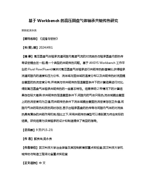
基于Workbench的高压圆盘气体轴承共轭传热研究郭良斌;吴永良【期刊名称】《润滑与密封》【年(卷),期】2024(49)1【摘要】高压圆盘气体轴承流道间隙内高速气流的对流换热与轴承圆盘内部热传导紧密耦合在一起,是一个典型的共轭传热问题。
基于ANSYS Workbench工作平台的Fluid Flow(Fluent)模块对高压圆盘气体轴承进行共轭传热数值模拟,获得轴承流道间隙内的速度和压力分布、流体域与固体域的温度分布以及共轭传热时流固耦合壁面的热流密度分布,并将其与非共轭传热恒温壁面条件下的计算结果进行对比,得到高压圆盘气体轴承共轭传热的一些基本特性。
结果表明:2种情况下的计算结果存在较大差异,非共轭传热恒温壁面条件下,间隙内的气体只吸热,流体域耦合壁面上的热流密度均为正值;而共轭传热条件下流体域耦合壁面热流密度存在正负值,间隙内气体的吸热和放热同时存在,显示出轴承圆盘的热传导与间隙内气体的对流换热具有复杂的共轭作用机制;相比之下,采用共轭传热模型可以得到更为符合实际的结果。
研究结果为该类轴承的设计和制造提供了有益的指导。
【总页数】9页(P15-23)【作者】郭良斌;吴永良【作者单位】武汉科技大学冶金装备及其控制教育部重点实验室;武汉科技大学机械传动与制造工程湖北省重点实验室【正文语种】中文【中图分类】TH133.35;V211.3【相关文献】1.基于ANSYS Workbench的气体静压轴承径向特性分析2.高压圆盘气体轴承可压缩边界层形态分析3.理想气体条件下平行圆盘止推气体轴承承载力特性研究4.不同供气总压下高压圆盘气体轴承边界层对流换热系数的研究5.基于Workbench 的高压圆盘气体轴承三维流场分析因版权原因,仅展示原文概要,查看原文内容请购买。
- 1、下载文档前请自行甄别文档内容的完整性,平台不提供额外的编辑、内容补充、找答案等附加服务。
- 2、"仅部分预览"的文档,不可在线预览部分如存在完整性等问题,可反馈申请退款(可完整预览的文档不适用该条件!)。
- 3、如文档侵犯您的权益,请联系客服反馈,我们会尽快为您处理(人工客服工作时间:9:00-18:30)。
图3操作项设置面板
设置流体域介质为air,固体域介质为默认的AL。
按图1所示边界条件设置计算域边界。
创建交界面,如图4所示进行设置。
图4设置交界面
4、初始化计算
设置初始化温度293K,如图5所示。
图5初始化面板
设置自动保存选项与动画录制项。
设置时间步长0.1s,时间步数100,内迭代次数20
图5简化模型
图6仿真模型
这幅图中可以看得更清楚,经过模型简化后,流体部分的外轮廓线是比较简洁的。注意这部分必须与齿轮箱贴合,这样以后计算热固耦合的时候,可以传递这个面上的温度场数据,如下图所示。这部分内容本帖中不涉及,本案例在流体外部用fluent的虚拟壁厚技术模拟一个壳体。
一些基础几何参数:
图7仿真模型与箱体示意图
我们首先来分析齿轮箱的结构,齿轮箱机械结构由壳体、端盖、大小齿轮、轴承、轴以及其他附件构成,我们首先要搞清楚分析的对象。壳体的温度是否是我们关注的要点?在本例中不是,那么我们的分析对象就是壳体中的所有元素,壳体只作为仿真的外边界。轴承和轴在仿真中的意义也不明显,因此我们都予以简化。
分析传热模型,齿轮摩擦生热是热源,这些热量通过几种方式传播:
网格划分完毕的效果如图:
图9整体网格
图10 局部网格
以上网格都是四面体单元,方便进行动网格设置。如不要求精确解,我们可以减小网格数目,采取以下这种单元数目较少的网格。可以看出,body之间的网格节点不共享。
图11简化网格
一些和网格划分有关的细节,可以按照这个表格去进行具体设置。这里的Advanced sizing功能一定要打开,否则在边角处生成的网格质量很差。表中用颜色标出了影响较大的设置项。
共轭传热计算
(2012-12-19 09:53:07)
转载▼
标签:
杂谈
分类:FLUENT技巧
共轭传热:流体传热与固体传热相互耦合。由于流体求解器同时具备流体与固体传热计算的能力,因此可以直接采用流体求解器进行求解,无需使用流固耦合计算。流体求解器能够求解流体对流、传导、辐射传热,对于固体传热计算,只能求解热传导方程。
3.2 湍流模型
标准k-ε模型用于强旋流,弯曲壁面流动或弯曲流线流动时,会产生一定的失真。因此采用RNGk-ε模型(Yakhot.Orzag)。与标准k-ε模型相比,RNG通过修正湍动粘度,考虑平均流动中的旋流流动情况,可以更好的处理高应变率以及流线弯曲程度较大的流动。
图16流线图
从流线图中容易看出,齿轮箱中的流体流线弯曲是很严重的,湍流模型必须做出调整。
udf见文后附件,热源大小假设是5000w/m3:
编译并且挂载udf以后,作为体积热源赋给固体域:
图12 体积热源设置
三、fluent仿真模型分析
图13 fluent中的模型
Fluent中整体模型如图所示。现在我们来分析具体设置。
3.1 壳体与边界处理
齿轮减速器的热量来自于齿轮啮合部位以及轴承,一般轴承产热约为齿轮啮合产热的1%,忽略。当齿轮减速器在某一工况下运转时,轴及滑油作为传热的媒介,将热量传导壳体,壳体又通过外部空气对流换热,与安装底座热传导。这里,壳体可以利用Fluent的带厚度壁面技术,虚拟一个壳体热阻,自定义换热系数,将壳体参数化处理。在Boundary Conditions中找到wall thickness的设置项,设置一个合理数值(30mm)即可。
1.热传导——从齿缘往齿轮中心传导
2.热对流——齿轮和润滑油,润滑油和空气,又称为共轭传热
3.热辐射——温度不高,辐射量小可忽略
因此,滑油和空气是传热的介质,必须在模型中考虑进去(事实上这部分传热达到91%)。滑油和空气是两相,因此要使用到fluent的多相流模型;要模拟甩油过程,要使用动网格模型;要模拟传热过程,利用fluent内建的传热模型。这三者是本案例的核心。
由于闭式传动风阻损失较小,忽略风阻损失。滑动和滚动损失分别由以下公式确定:
齿轮滚动和滑动摩擦损失分配到啮合的两齿轮关系式:
通过公式计算生热过程不再赘述。生热的施加在本例中是一个重点,因为使用了交界面进行热交换,并且兼容动网格,但是fluent不支持在交界面上施加热源,因此我们要计算出生热量,作为体积热源施加到齿轮固体域上。
基于
2015-12-08 17:45:383966
简介:
今天为大家带来齿轮箱瞬态温度场仿真的原创案例。限于篇幅,这个帖子不像之前一样把所有设置一步步贴图,因此只给出关键图,设置全部给出了表格形式。图1和图23是动图,但是好像帖子里动不起来,可以点击我的头像——作品展示里有动态图。
图1 齿轮箱甩油润滑
图4流体仿真流程
一、模型简化与网格划分
由于复杂的三维结构会增加网格划分的难度,会导致网格数目的无谓增加,加大计算量,因此对齿轮减速器三维模型进行简化:壳体的凸台、通孔、垫圈等予以去除;统一壁面厚度;滚动轴承结构在对应位置采取同心圆环来表示,方便施加热流。这里的模型简化工作是用SpaceClaim做的。简化后的模型如图所示:
这里不得不提到两位外国学者,Guillaume Houzeaux对齿轮泵进行了仿真,并且关注局部网格,这可能是最早对齿轮+流体进行仿真;而F.Lemfeld率先采用两相流模型捕捉了齿轮箱内的流体瞬态变化情况,但他在网格方面的处理比较简单,对齿轮齿形进行了切除,同时使用一定的壁面粗糙度值模拟齿形的存在,使齿轮能够甩油。
为所有边界命名,尤其是流体和固体区域交界面,后面需要在求解器中进行设置。
3、进入Fluent求解设置
本例为瞬态计算。
涉及到热量传递,因此需要激活能量方程。
流体介质为理想气体,考虑其在温度影响下密度变化。
考虑重力影响,设置重力加速度向量[0,-9.81,0],设置操作密度为0。如图3所示。
压力-速度耦合方程采用PISO求解方式,对流项计算采用QUICK算法,其他项采用二阶迎风格式。
在fluent中导入网格以后,第一步一定要进行网格检查。
注意几个参数的数值,如果太差,动网格部分可能会报错,一般是出现负体积。
二、产热分析
齿轮传动的产热主要来源是齿轮啮合产热。这部分的产热以目前的技术手段难以从仿真直接获得,但是有相应的经验模型,经验模型计算方便,模型中相关系数的获得比较容易。Anderson和Loewenthal法将齿轮的功率分为三部分,滑动、滚动和风阻损失。
说了这么多废话,现在回到主题。
图3 流固热耦合仿真流程
本例需要用到的模块包括fluent模块,其中又集成了ansys自带的几何处理与网格划分工具。后面与fluent共享结果的是稳态热分析模块,以及静力结构模块,用来分析热应力对结构的影响,如用来分析热变形,限于篇幅本例不涉及。本例实际流程可以简化如下,我个人喜欢拆分不同的模块,这样方便“故障隔离”:
这里要准确理解ANSYS WORKBENCH的part意义,将建模时不同的body放在一个part下与不放在一个part下有什么区别?很多新手都会遇到这个问题,至少我是这么走过来的,但是没看到有任何一本书讲清楚了这个问题。其实,其区别简单来看就是节点是否共享。
图8网格节点是否共享的区别
这里我简单画了一个示意图(画的比较难看),从图中可以看出二者的区别。两种方法在fluent中的区别是:前者流体与固体网格节点共享,在fluent中会自动对命名完毕的固体域生成shadow面,比如driven-shadow。若不放在一个part下,fluent会自动检测各个part(独立几何结构视作一个part)之间的接触区域(其实此部分工作在meshing中完成),对contact region生成interface。Interface就是交界面,这个面在fluent中可以用来传递域间参数,如压力、热等。
齿轮传动的核心是齿轮副,对此不做任何简化以保证计算结果精度。但是渐开线齿轮在现实中在节圆啮合,那么两齿轮中间的网格最小处趋近于0,无法划分网格。目前通用的手段就是拉大中心距,只需将二齿轮中间拉大适当距离,保证有2-3层网格即可。这个改动的影响在可接受范围内。
网格划分采用ANSYS自带Meshing模块,先压制齿轮固体,再将齿轮齿形处进行一定细化,流体固体域分别划分网格。
图14虚拟壳体设置
固体域和流体域的换热前文已经说过,通过交界面进行:
图15交界面设置
注意这里交界面的两侧,fluent已经自动为其加后缀命名进行区分,一个是源面,一个是目标面。当然你也可以在上一步划分网格的时候就自己命名,这样更有利于辨识。比如我这里一个面叫做driven,一个叫做driven-fluid,代表与小齿轮接触的流体表面。
本例演示共轭传热问题在FLUENT中的求解方法。
1、问题描述
如图1所示的计算区域,既包含流体区域也包含固体区域。在初始状态下,流体域与固体与温度均为293K,然后给固体域底部施加恒定温度434K,计算分析计算域内温度随时间分布规律。边界条件如图中所示。
图1计算域描述
2、建立几何模型并划分网格
利用DM建立如图1所示2D平面几何。采用全四边形网格划分,如图2所示。
—————————————————————————————————————————————
正文:
齿轮温度场涉及到摩擦学、传热学、机械传动理论和有限元分析等多学科领域的知识,是一个比较复杂的问题。
1969年,Blok.H阐述了热网络理论,其本质是考虑系统中各部分生热,在网络中用一个节点表示,每个节点表示每部分的平均温度。通过整体分析得到要求的的各部分的温度值。这种方法的缺陷在于,首先必须建立热阻、功率损失、对流换热系数计算模型,而这些参数不容易获得。那么我们考虑用仿真的手段去求解这个问题。
齿轮减速结构是机械传动中最常见的形式,如下图。
图2齿轮箱结构
由于齿轮之间存在摩擦,因此齿轮系统的温度场必须进行关注,以确保:
o齿轮结构没有过热(overheating)