计算机科学与技术专业外文翻译--插值与拟合
《计算机专业英语》(中英文对照)
计算机专业英语
1-4
Chapter 1 The History and Future of Computers
1.1 The Invention of the Computer
It is hard to say exactly when the modern computer was invented. Starting in the 1930s and through the 1940s, a number of machines were developed that were like computers. But most of these machines did not have all the characteristics that we associate with computers today. These characteristics are that the machine is electronic, that it has a stored program, and that it is general purpose.
计算机专业英语 Computer English
Chapter 1 The History and Future of Computers 2009.9.1
Chapter 1 The History and Future of Computers
Key points: useful terms and definitions of
在 EDVAC 完 成 之 前 , 其 他 一 些 机 器 建 成 了 , 它 们 吸 收 了 Eckert 、 Mauchly和Neuman设计的要素。其中一部是在英国剑桥研制的电子延迟 存储自动计算机,或简称EDSAC,它在1949年5月首次运行,它可能是世 界的第一台电子储存程序、通用型计算机投入运行。在美国运行的第一 部计算机是二进制自动计算机,或简称BINAC,它在1949年8月投入运行。
计算机科学与技术专业课程英译

1 计算机导论Intorduction of Computer2 高等数学Avanced Mathematics3 线性代数Linear Alberia4 离散数学Discrete Mathematics5 数值分析Numerical value Analysis6 大学英语Colleage English7 模拟电子电路Analog Electronic Circuit8 数字电子电路Digital Electronic Circuit9 软件工程Software Engineering10 信号与系统Signal and System11 多媒体技术Multimedia Technology12 操作系统Operation System13 数据结构Data Structure14 编译原理Principle of Compiling15 数据库原理Principle of Database16 信号与系统Signal and System17 计算机组成原理Constitution Principle of Computer18 计算机网络Cyber networks19 计算机图形学Cyber graphics20 人工智能Artificial Intelligence21 C++语言程序设计C++ Program Design22J AVA语言程序设计Java Program Design23 ASP编程基础及应用ASP Programming Base and Application24 LINUX操作系统应用与开发Linux Operation System Application and Development25 微机原理Principle of Micro computer资源与环境经济学Economics of Natural Resources and The Environment劳动经济学Labor Economics经济学名著选读Selected Reading of the Masterpieces of Economics社会主义经济理论Socialist Economic Theory国际银行学International Banking城市经济学Urban Economics精益管理Lean Management管理学Management计算机外设原理与维修Computer Peripheral。
数值计算方法插值与拟合

数值计算方法插值与拟合数值计算方法在科学计算和工程应用中起着重要的作用,其中插值和拟合是其中两个常用的技术。
插值是指通过已知的离散数据点来构造出连续函数或曲线的过程,拟合则是找到逼近已知数据的函数或曲线。
本文将介绍插值和拟合的基本概念和常见的方法。
一、插值和拟合的基本概念插值和拟合都是通过已知数据点来近似表达未知数据的方法,主要区别在于插值要求通过已知数据点的函数必须经过这些数据点,而拟合则只要求逼近这些数据点。
插值更加精确,但是可能会导致过度拟合;拟合则更加灵活,能够通过调整参数来平衡拟合精度和模型复杂度。
二、插值方法1. 线性插值线性插值是一种简单的插值方法,通过已知数据点构造出线段,然后根据插值点在线段上进行线性插值得到插值结果。
2. 拉格朗日插值拉格朗日插值是一种基于多项式插值的方法,通过已知数据点构造出一个多项式,并根据插值点求解插值多项式来得到插值结果。
3. 分段线性插值分段线性插值是一种更加灵活的插值方法,通过将插值区间分成若干小段,然后在每个小段上进行线性插值。
三、拟合方法1. 最小二乘法拟合最小二乘法是一种常用的拟合方法,通过最小化实际观测点和拟合函数之间的残差平方和来确定拟合函数的参数。
2. 多项式拟合多项式拟合是一种基于多项式函数的拟合方法,通过选择合适的多项式次数来逼近已知数据点。
3. 曲线拟合曲线拟合是一种更加灵活的方法,通过选择合适的曲线函数来逼近已知数据点,常见的曲线包括指数曲线、对数曲线和正弦曲线等。
四、插值与拟合的应用场景插值和拟合在实际应用中具有广泛的应用场景,比如图像处理中的图像重建、信号处理中的滤波器设计、金融中的风险评估等。
五、插值与拟合的性能评价插值和拟合的性能可以通过多种指标进行评价,常见的评价指标包括均方根误差、相关系数和拟合优度等。
六、总结插值和拟合是数值计算方法中常用的技术,通过已知数据点来近似表达未知数据。
插值通过已知数据点构造出连续函数或曲线,拟合则找到逼近已知数据的函数或曲线。
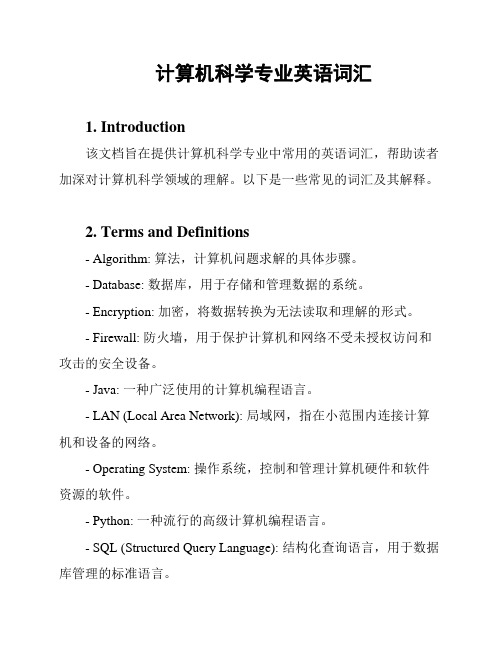
计算机科学专业英语词汇
计算机科学专业英语词汇
1. Introduction
该文档旨在提供计算机科学专业中常用的英语词汇,帮助读者加深对计算机科学领域的理解。
以下是一些常见的词汇及其解释。
2. Terms and Definitions
- Algorithm: 算法,计算机问题求解的具体步骤。
- Database: 数据库,用于存储和管理数据的系统。
- Encryption: 加密,将数据转换为无法读取和理解的形式。
- Firewall: 防火墙,用于保护计算机和网络不受未授权访问和攻击的安全设备。
- Java: 一种广泛使用的计算机编程语言。
- LAN (Local Area Network): 局域网,指在小范围内连接计算机和设备的网络。
- Operating System: 操作系统,控制和管理计算机硬件和软件资源的软件。
- Python: 一种流行的高级计算机编程语言。
- SQL (Structured Query Language): 结构化查询语言,用于数据库管理的标准语言。
- Virtual Reality: 虚拟现实,一种模拟现实环境的计算机技术。
3. Conclusion
通过掌握这些常用计算机科学专业英语词汇,读者可以更好地理解和应用计算机科学领域的知识。
在研究和实践中,不断积累和扩充词汇量将有助于提升专业能力和沟通交流能力。
希望这份文档能对您有所帮助!。
插值和拟合区别

>> [xx,res]=lsqcurvefit(f,[1,1,1,1,1],x,y); xx',res
Optimization terminated successfully: Relative function value changing by less than
125.29*x^4+74.450*x^327.672*x^2+4.9869*x+.42037e-6
最小二乘曲线拟合
• 格式: [a, jm]=lsqcurvefit(Fun,a0,x,y)
例 >> x=0:.1:10; >> y=0.12*exp(-0.213*x)+0.54*exp(-0.17*x).*sin(1.23*x);
2*x0).*exp(-4*x0) x0.^2]; >> y1=A1*c; >> plot(x0,y1,x,y,'x')
例
• 数据分析
>> x=[1.1052,1.2214,1.3499,1.4918,1.6487,1.8221,2.0138,... 2.2255,2.4596,2.7183,3.6693];
0.1200 0.2130 0.5400 0.1700 1.2300 res = 9.5035e-021
• 绘制曲线: >> x1=0:0.01:10; y1=f(xx,x1); plot(x1,y1,x,y,'o')
计算机科学与技术专业英语

计算机科学与技术专业英语Computer Science and Technology Major计算机科学与技术专业(jìsuànjī kēxué yǔ jìshù zhuānyè) - Computer Science and Technology Major计算机科学与技术(Computer Science and Technology)是计算机科学与技术学科的核心专业,主要培养学生具有计算机科学与技术专业的基本理论、基本知识和基本技能,能够在计算机科学与技术领域从事应用与开发、设计与实施、管理与服务等工作。
Computer Science and Technology is a core major in the field of computer science and technology. It mainly focuses on cultivating students with basic theories, knowledge, and skills in computer science and technology. Graduates will be able to engage in application development, design and implementation, management, and service in the field of computer science and technology.专业课程(zhuānyè kèchéng) - Major Courses计算机科学与技术专业的课程包括但不限于以下方面:The courses of the Computer Science and Technology major include but are not limited to the following aspects:1.基础课程(basic courses):- 计算机组成原理(Computer Organization and Architecture)- 数据结构与算法(Data Structures and Algorithms)- 操作系统(Operating Systems)- 离散数学(Discrete Mathematics)- 编译原理(Compiler Design)- 计算机网络(Computer Networks)2.核心课程(core courses):- 计算机图形学(Computer Graphics)- 数据库系统(Database Systems)- 人工智能(Artificial Intelligence)- 计算机安全(Computer Security)- 软件工程(Software Engineering)- 分布式系统(Distributed Systems)3.专业选修课程(major elective courses):- 数据挖掘(Data Mining)- 机器学习(Machine Learning)- 物联网技术(Internet of Things)- 云计算(Cloud Computing)- 嵌入式系统(Embedded Systems)就业方向(jiùyè fāngxiàng) - Career Paths计算机科学与技术专业的毕业生在以下领域有广泛的就业机会: Graduates of the Computer Science and Technology major have extensive job opportunities in the following fields:- 软件开发(Software Development)- 网络安全(Network Security)- 数据分析(Data Analysis)- 人工智能与机器学习(Artificial Intelligence and Machine Learning)- 云计算与大数据(Cloud Computing and Big Data)- 嵌入式系统开发(Embedded System Development)- 网站设计与开发(Website Design and Development)- IT管理与咨询(IT Management and Consulting)以上是关于计算机科学与技术专业的简单介绍。
计算机专业毕业论文外文翻译
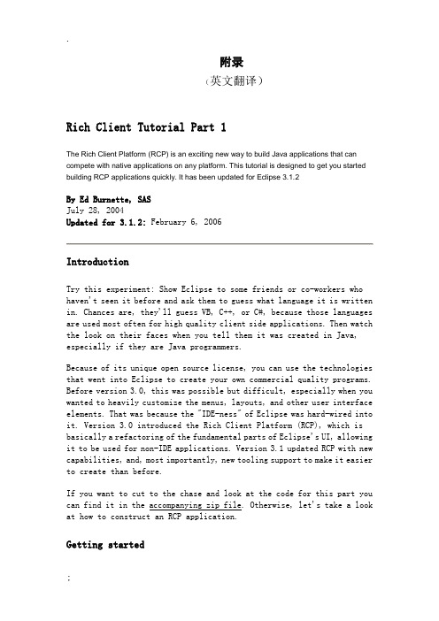
附录(英文翻译)Rich Client Tutorial Part 1The Rich Client Platform (RCP) is an exciting new way to build Java applications that can compete with native applications on any platform. This tutorial is designed to get you started building RCP applications quickly. It has been updated for Eclipse 3.1.2By Ed Burnette, SASJuly 28, 2004Updated for 3.1.2: February 6, 2006IntroductionTry this experiment: Show Eclipse to some friends or co-workers who haven't seen it before and ask them to guess what language it is written in. Chances are, they'll guess VB, C++, or C#, because those languages are used most often for high quality client side applications. Then watch the look on their faces when you tell them it was created in Java, especially if they are Java programmers.Because of its unique open source license, you can use the technologies that went into Eclipse to create your own commercial quality programs. Before version 3.0, this was possible but difficult, especially when you wanted to heavily customize the menus, layouts, and other user interface elements. That was because the "IDE-ness" of Eclipse was hard-wired into it. Version 3.0 introduced the Rich Client Platform (RCP), which is basically a refactoring of the fundamental parts of Eclipse's UI, allowing it to be used for non-IDE applications. Version 3.1 updated RCP with new capabilities, and, most importantly, new tooling support to make it easier to create than before.If you want to cut to the chase and look at the code for this part you can find it in the accompanying zip file. Otherwise, let's take a look at how to construct an RCP application.Getting startedRCP applications are based on the familiar Eclipse plug-in architecture, (if it's not familiar to you, see the references section). Therefore, you'll need to create a plug-in to be your main program. Eclipse's Plug-in Development Environment (PDE) provides a number of wizards and editors that take some of the drudgery out of the process. PDE is included with the Eclipse SDK download so that is the package you should be using. Here are the steps you should follow to get started.First, bring up Eclipse and select File > New > Project, then expand Plug-in Development and double-click Plug-in Project to bring up the Plug-in Project wizard. On the subsequent pages, enter a Project name such as org.eclipse.ui.tutorials.rcp.part1, indicate you want a Java project, select the version of Eclipse you're targeting (at least 3.1), and enable the option to Create an OSGi bundle manifest. Then click Next >.Beginning in Eclipse 3.1 you will get best results by using the OSGi bundle manifest. In contrast to previous versions, this is now the default.In the next page of the Wizard you can change the Plug-in ID and other parameters. Of particular importance is the question, "Would you like to create a rich client application?". Select Yes. The generated plug-in class is optional but for this example just leave all the other options at their default values. Click Next > to continue.If you get a dialog asking if Eclipse can switch to the Plug-in Development Perspective click Remember my decision and select Yes (this is optional).Starting with Eclipse 3.1, several templates have been provided to make creating an RCP application a breeze. We'll use the simplest one available and see how it works. Make sure the option to Create a plug-in using one of the templates is enabled, then select the Hello RCP template. This isRCP's equivalent of "Hello, world". Click Finish to accept all the defaults and generate the project (see Figure 1). Eclipse will open the Plug-in Manifest Editor. The Plug-in Manifest editor puts a friendly face on the various configuration files that control your RCP application.Figure 1. The Hello World RCP project was created by a PDE wizard.Taking it for a spinTrying out RCP applications used to be somewhat tedious. You had to create a custom launch configuration, enter the right application name, and tweak the plug-ins that were included. Thankfully the PDE keeps track of all this now. All you have to do is click on the Launch an Eclipse Application button in the Plug-in Manifest editor's Overview page. You should see a bare-bones Workbench start up (see Figure 2).Figure 2. By using thetemplates you can be up andrunning anRCPapplication inminutes.Making it aproductIn Eclipse terms a product is everything that goes with your application, including all the other plug-ins it depends on, a command to run the application (called the native launcher), and any branding (icons, etc.) that make your application distinctive. Although as we've just seen you can run a RCP application without defining a product, having one makes it a whole lot easier to run the application outside of Eclipse. This is one of the major innovations that Eclipse 3.1 brought to RCP development.Some of the more complicated RCP templates already come with a product defined, but the Hello RCP template does not so we'll have to make one.In order to create a product, the easiest way is to add a product configuration file to the project. Right click on the plug-in project and select New > Product Configuration. Then enter a file name for this new configuration file, such as part1.product. Leave the other options at their default values. Then click Finish. The Product Configuration editor will open. This editor lets you control exactly what makes up your product including all its plug-ins and branding elements.In the Overview page, select the New... button to create a new product extension. Type in or browse to the defining plug-in(org.eclipse.ui.tutorials.rcp.part1). Enter a Product ID such as product, and for the Product Application selectorg.eclipse.ui.tutorials.rcp.part1.application. Click Finish to define the product. Back in the Overview page, type in a new Product Name, for example RCP Tutorial 1.In Eclipse 3.1.0 if you create the product before filling inthe Product Name you may see an error appear in the Problems view. The error will go away when you Synchronize (see below). This is a known bug that is fixed in newer versions. Always use the latest available maintenance release for the version of Eclipse you're targeting!Now select the Configuration tab and click Add.... Select the plug-in you just created (org.eclipse.ui.tutorials.rcp.part1) and then click on Add Required Plug-ins. Then go back to the Overview page and press Ctrl+S or File > Save to save your work.If your application needs to reference plug-ins that cannot be determined until run time (for example the tomcat plug-in), then add them manually in the Configuration tab.At this point you should test out the product to make sure it runs correctly. In the Testing section of the Overview page, click on Synchronize then click on Launch the product. If all goes well, the application should start up just like before.Plug-ins vs. featuresOn the Overview page you may have noticed an option that says the product configuration is based on either plug-ins or features. The simplest kind of configuration is one based on plug-ins, so that's what this tutorial uses. If your product needs automatic update or Java Web Start support, then eventually you should convert it to use features. But take my advice and get it working without them first.Running it outside of EclipseThe whole point of all this is to be able to deploy and run stand-alone applications without the user having to know anything about the Java and Eclipse code being used under the covers. For a real application you may want to provide a self-contained executable generated by an install program like InstallShield or NSIS. That's really beyond the scope of this article though, so we'll do something simpler.The Eclipse plug-in loader expects things to be in a certain layout so we'll need to create a simplified version of the Eclipse install directory. This directory has to contain the native launcher program, config files,and all the plug-ins required by the product. Thankfully, we've given the PDE enough information that it can put all this together for us now.In the Exporting section of the Product Configuration editor, click the link to Use the Eclipse Product export wizard. Set the root directory to something like RcpTutorial1. Then select the option to deploy into a Directory, and enter a directory path to a temporary (scratch) area such as C:\Deploy. Check the option to Include source code if you're building an open source project. Press Finish to build and export the program.The compiler options for source and class compatibility in the Eclipse Product export wizard will override any options you have specified on your project or global preferences. As part of the Export process, the plug-in is code is recompiled by an Ant script using these options.The application is now ready to run outside Eclipse. When you're done you should have a structure that looks like this in your deployment directory:RcpTutorial1| .eclipseproduct| eclipse.exe| startup.jar+--- configuration| config.ini+--- pluginsmands_3.1.0.jarorg.eclipse.core.expressions_3.1.0.jarorg.eclipse.core.runtime_3.1.2.jarorg.eclipse.help_3.1.0.jarorg.eclipse.jface_3.1.1.jarorg.eclipse.osgi_3.1.2.jarorg.eclipse.swt.win32.win32.x86_3.1.2.jarorg.eclipse.swt_3.1.0.jarorg.eclipse.ui.tutorials.rcp.part1_1.0.0.jarorg.eclipse.ui.workbench_3.1.2.jarorg.eclipse.ui_3.1.2.jarNote that all the plug-ins are deployed as jar files. This is the recommended format starting in Eclipse 3.1. Among other things this saves disk space in the deployed application.Previous versions of this tutorial recommended using a batch file or shell script to invoke your RCP program. It turns out this is a bad idea because you will not be able to fully brand your application later on. For example, you won't be able to add a splash screen. Besides, theexport wizard does not support the batch file approach so just stick with the native launcher.Give it a try! Execute the native launcher (eclipse or eclipse.exe by default) outside Eclipse and watch the application come up. The name of the launcher is controlled by branding options in the product configuration.TroubleshootingError: Launching failed because the org.eclipse.osgi plug-in is not included...You can get this error when testing the product if you've forgotten to list the plug-ins that make up the product. In the Product Configuration editor, select the Configuration tab, and add all your plug-ins plus all the ones they require as instructed above.Compatibility and migrationIf you are migrating a plug-in from version 2.1 to version 3.1 there are number of issues covered in the on-line documentation that you need to be aware of. If you're making the smaller step from 3.0 to 3.1, the number of differences is much smaller. See the References section for more information.One word of advice: be careful not to duplicate any information in both plug-in.xml and MANIFEST.MF. Typically this would not occur unless you are converting an older plug-in that did not use MANIFEST.MF into one that does, and even then only if you are editing the files by hand instead of going through the PDE.ConclusionIn part 1 of this tutorial, we looked at what is necessary to create a bare-bones Rich Client application. The next part will delve into the classes created by the wizards such as the WorkbenchAdvisor class. All the sample code for this part may be found in the accompanying zip file.ReferencesRCP Tutorial Part 2RCP Tutorial Part 3Eclipse Rich Client PlatformRCP Browser example (project org.eclipse.ui.examples.rcp.browser)PDE Does Plug-insHow to Internationalize your Eclipse Plug-inNotes on the Eclipse Plug-in ArchitecturePlug-in Migration Guide: Migrating to 3.1 from 3.0Plug-in Migration Guide: Migrating to 3.0 from 2.1译文:Rich Client教程第一部分The Rich Client Platform (RCP)是一种创建Java应用程序的令人兴奋的新方法,可以和任何平台下的自带应用程序进行竞争。
计算机专业外文资料翻译
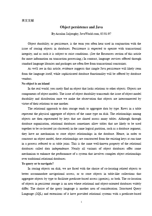
英文文献Object persistence and JavaBy Arsalan Saljoughy, , 05/01/97Object durability, or persistence, is the term you often hear used in conjunction with the issue of storing objects in databases. Persistence is expected to operate with transactional integrity, and as such it is subject to strict conditions. (See the Resources section of this article for more information on transaction processing.) In contrast, language services offered through standard language libraries and packages are often free from transactional constraints.As we'll see in this article, evidence suggests that simple Java persistence will likely stem from the language itself, while sophisticated database functionality will be offered by database vendors.No object is an islandIn the real world, you rarely find an object that lacks relations to other objects. Objects are components of object models. The issue of object durability transcends the issue of object model durability and distribution once we make the observation that objects are interconnected by virtue of their relations to one another.The relational approach to data storage tends to aggregate data by type. Rows in a table represent the physical aggregate of objects of the same type on disk. The relationships among objects are then represented by keys that are shared across many tables. Although through database organization, relational databases sometimes allow tables that are likely to be used together to be co-located (or clustered) in the same logical partition, such as a database segment, they have no mechanism to store object relationships in the database. Hence, in order to construct an object model, these relationships are constructed from the existing keys at run time in a process referred to as table joins. This is the same well-known property of the relational databases called data independence. Nearly all variants of object databases offer some mechanism to enhance the performance of a system that involves complex object relationships over traditional relational databases.To query or to navigate?In storing objects on disk, we are faced with the choice of co-locating related objects to better accommodate navigational access, or to store objects in table-like collections that aggregate objects by type to facilitate predicate-based access (queries), or both. The co-location of objects in persistent storage is an area where relational and object-oriented databases widely differ. The choice of the query language is another area of consideration. Structured Query Language (SQL) and extensions of it have provided relational systems with a predicate-basedaccess mechanism. Object Query Language (OQL) is an object variant of SQL, standardized by ODMG, but support for this language is currently scant. Polymorphic methods offer unprecedented elegance in constructing a semantic query for a collection of objects. For example, imagine a polymorphic behavior for acccount called isInGoodStanding. It may return the Boolean true for all accounts in good standing, and false otherwise. Now imagine the elegance of querying the collection of accounts, where inGoodStanding is implemented differently based on business rules, for all accounts in good standing. It may look something like:setOfGoodCustomers = setOfAccounts.query(account.inGoodStanding());While several of the existing object databases are capable of processing such a query style in C++ and Smalltalk, it is difficult for them to do so for larger (say, 500+ gigabytes) collections and more complex query expressions. Several of the relational database companies, such as Oracle and Informix, will soon offer other, SQL-based syntax to achieve the same result. Persistence and typeAn object-oriented language aficionado would say persistence and type are orthogonal properties of an object; that is, persistent and transient objects of the same type can be identical because one property should not influence the other. The alternative view holds that persistence is a behavior supported only by persistable objects and certain behaviors may apply only to persistent objects. The latter approach calls for methods that instruct persistable objects to store and retrieve themselves from persistent storage, while the former affords the application a seamless view of the entire object model -- often by extending the virtual memory system. Canonicalization and language independenceObjects of the same type in a language should be stored in persistent storage with the same layout, regardless of the order in which their interfaces appear. The processes of transforming an object layout to this common format are collectively known as canonicalization of object representation. In compiled languages with static typing (not Java) objects written in the same language, but compiled under different systems, should be identically represented in persistent storage.An extension of canonicalization addresses language-independent object representation. If objects can be represented in a language-independent fashion, it will be possible for different representations of the same object to share the same persistent storage.One mechanism to accomplish this task is to introduce an additional level of indirection through an interface definition language (IDL). Object database interfaces can be made through the IDL and the corresponding data structures. The downside of IDL style bindings is two fold: First, the extra level of indirection always requires an additional level of translation, which impacts the overall performance of the system; second, it limits use of database services that are unique to particular vendors and that might be valuable to application developers.A similar mechanism is to support object services through an extension of the SQL. Relational database vendors and smaller object/relational vendors are proponents of this approach; however, how successful these companies will be in shaping the framework for object storage remains to be seen.But the question remains: Is object persistence part of the object's behavior or is it an external service offered to objects via separate interfaces? How about collections of objects and methods for querying them? Relational, extended relational, and object/relational approaches tend to advocate a separation between language, while object databases -- and the Java language itself -- see persistence as intrinsic to the language:Native Java persistence via serializationObject serialization is the Java language-specific mechanism for the storage and retrieval of Java objects and primitives to streams. It is worthy to note that although commercial third-party libraries for serializing C++ objects have been around for some time, C++ has never offered a native mechanism for object serialization. Here's how to use Java's serialization: // Writing "foo" to a stream (for example, a file)// Step 1. Create an output stream// that is, create bucket to receive the bytesFileOutputStream out = new FileOutputStream("fooFile");// Step 2. Create ObjectOutputStream// that is, create a hose and put its head in the bucketObjectOutputStream os = new ObjectOutputStream(out)// Step 3. Write a string and an object to the stream// that is, let the stream flow into the bucketos.writeObject("foo");os.writeObject(new Foo());// Step 4. Flush the data to its destinationos.flush();The Writeobject method serializes foo and its transitive closure -- that is, all objects that can be referenced from foo within the graph. Within the stream only one copy of the serialized object exists. Other references to the objects are stored as object handles to save space and avoid circular references. The serialized object starts with the class followed by the fields of each class in the inheritance hierarchy.// Reading an object from a stream// Step 1. Create an input streamFileInputStream in = new FileInputStream("fooFile");// Step 2. Create an object input streamObjectInputStream ins = new ObjectInputStream(in);// Step 3. Got to know what you are readingString fooString = (String)ins.readObject();Foo foo = (Foo)s.readObject();Object serialization and securityBy default, serialization writes and reads non-static and non-transient fields from the stream. This characteristic can be used as a security mechanism by declaring fields that may not be serialized as private transient. If a class may not be serialized at all, writeObject and readObject methods should be implemented to throw NoAccessException.Persistence with transactional integrity: Introducing JDBCModeled after X/Open's SQL CLI (Client Level Interface) and Microsoft's ODBC abstractions, Java database connectivity (JDBC) aims to provide a database connectivity mechanism that is independent of the underlying database management system (DBMS).To become JDBC-compliant, drivers need to support at least the ANSI SQL-2 entry-level API, which gives third-party tool vendors and applications enough flexibility for database access.JDBC is designed to be consistent with the rest of the Java system. Vendors are encouraged to write an API that is more strongly typed than ODBC, which affords greater static type-checking at compile time.Here's a description of the most important JDBC interfaces:java.sql.Driver.Manager handles the loading of drivers and provides support for new database connections.java.sql.Connection represents a connection to a particular database.java.sql.Statement acts as a container for executing an SQL statement on a given connection.java.sql.ResultSet controls access to the result set.You can implement a JDBC driver in several ways. The simplest would be to build the driver as a bridge to ODBC. This approach is best suited for tools and applications that do not require high performance. A more extensible design would introduce an extra level of indirection to the DBMS server by providing a JDBC network driver that accesses the DBMS server through a published protocol. The most efficient driver, however, would directly access the DBMS proprietary API.Object databases and Java persistenceA number of ongoing projects in the industry offer Java persistence at the object level. However, as of this writing, Object Design's PSE (Persistent Storage Engine) and PSE Pro are the only fully Java-based, object-oriented database packages available (at least, that I am aware of). Check the Resources section for more information on PSE and PSE Pro.Java development has led to a departure from the traditional development paradigm for software vendors, most notably in the development process timeline. For example, PSE and PSE Pro are developed in a heterogeneous environment. And because there isn't a linking step in the development process, developers have been able to create various functional components independent of each other, which results in better, more reliable object-oriented code.PSE Pro has the ability to recover a corrupted database from an aborted transaction caused by system failure. The classes that are responsible for this added functionality are not present in the PSE release. No other differences exist between the two products. These products are what we call "dribbleware" -- software releases that enhance their functionality by plugging in new components. In the not-so-distant future, the concept of purchasing large, monolithic software would become a thing of the past. The new business environment in cyberspace, together with Java computing, enable users to purchase only those parts of the object model (object graph) they need, resulting in more compact end products.PSE works by post-processing and annotating class files after they have been created by the developer. From PSE's point of view, classes in an object graph are either persistent-capable or persistent-aware. Persistent-capable classes may persist themselves while persistent-aware classes can operate on persistent objects. This distinction is necessary because persistence may not be a desired behavior for certain classes. The class file post-processor makes the following modifications to classes:Modifies the class to inherit from odi.Persistent or odi.util.HashPersistent.Defines the initializeContents() method to load real values into hollow instances of your Persistent subclass. ObjectStore provides methods on the GenericObject class that retrieves each Field type.Be sure to call the correct methods for the fields in your persistent object. A separate method is available for obtaining each type of Field object. ObjectStore calls the initializeContents() method as needed. The method signature is:public void initializeContents(GenericObject genObj)Defines the flushContents() method to copy values from a modified instance (active persistent object) back to the database. ObjectStore provides methods on the GenericObject Be sure to call the correct methods for the fields in your persistent object. A separate method is available for setting each type of Field object. ObjectStore calls the flushContents() method as needed. The method signature is:public void flushContents(GenericObject genObj)Defines the clearContents() method to reset the values of an instance to the default values. This method must set all reference fields that referred to persistent objects to null. ObjectStore calls this method as needed. The method signature is:public void clearContents()Modifies the methods that reference non-static fields to call the Persistent.fetch() and Persistent.dirty() methods as needed. These methods must be called before the contents of persistent objects can be accessed or modified, respectively. While this step is not mandatory, it does provide a systematic way to ensure that the fetch() or dirty() method is called prior to accessing or updating object content.Defines a class that provides schema information about the persistence-capable class.All these steps can be completed either manually or automatically.PSE's transaction semanticYou old-time users of ObjectStore probably will find the database and transaction semantics familiar. There is a system-wide ObjectStore object that initializes the environment and is responsible for system-wide parameters. The Database class offers methods (such as create, open, and close), and the Transaction class has methods to begin, abort, or commit transactions. As with serialization, you need to find an entry point into the object graph. The getRoot and setRoot methods of the Database class serve this function. I think a few examples would be helpful here. This first snippet shows how to initialize ObjectStore:ObjectStore.initialize(serverName, null);try {db = Database.open(dbName, Database.openUpdate);} catch(DatabaseNotFoundException exception) {db = Database.create(dbName, 0664);}This next snippet shows how to start and commit a transaction:Transaction transaction = Transaction.begin(Transaction.update);try {foo = (Foo)db.getRoot("fooHead");} catch(DatabaseRootNotFoundException exception) {db.createRoot("fooHead", new Foo());}mit();The three classes specified above -- Transaction, Database, and ObjectStore -- are fundamental classes for ObjectStore. PSE 1.0 does not support nested transactions, backup and recovery, clustering, large databases, object security beyond what is available in the language, and any type of distribution. What is exciting, however, is all of this functionality will be incrementally added to the same foundation as the product matures.About the authorArsalan Saljoughy is asystems engineer specializing in object technology at Sun Microsystems. He earned his M.S. in mathematics from SUNY at Albany, and subsequently was a research fellow at the University of Berlin. Before joining Sun, he worked as a developer and as an IT consultant to financial services companies.ConclusionAlthough it is still too early to establish which methodology for object persistence in general and Java persistence in particular will be dominant in the future, it is safe to assume that a myriad of such styles will co-exist. The shift of storing objects as objects without disassembly into rows and columns is sure to be slow, but it will happen. In the meantime, we are more likely to see object databases better utilized in advanced engineering and telecommunications applications than in banking and back-office financial applications.英文翻译对象持久化和Java-深入的了解面向对象语言中的对象持久的讨论Arsalan Saljoughy,, 05/01/97对象持久化这个术语你常常会和数据存储一起听到。
计算机科学与技术 外文翻译 英文文献 中英对照

附件1:外文资料翻译译文大容量存储器由于计算机主存储器的易失性和容量的限制, 大多数的计算机都有附加的称为大容量存储系统的存储设备, 包括有磁盘、CD 和磁带。
相对于主存储器,大的容量储存系统的优点是易失性小,容量大,低成本, 并且在许多情况下, 为了归档的需要可以把储存介质从计算机上移开。
术语联机和脱机通常分别用于描述连接于和没有连接于计算机的设备。
联机意味着,设备或信息已经与计算机连接,计算机不需要人的干预,脱机意味着设备或信息与机器相连前需要人的干预,或许需要将这个设备接通电源,或许包含有该信息的介质需要插到某机械装置里。
大量储存器系统的主要缺点是他们典型地需要机械的运动因此需要较多的时间,因为主存储器的所有工作都由电子器件实现。
1. 磁盘今天,我们使用得最多的一种大量存储器是磁盘,在那里有薄的可以旋转的盘片,盘片上有磁介质以储存数据。
盘片的上面和(或)下面安装有读/写磁头,当盘片旋转时,每个磁头都遍历一圈,它被叫作磁道,围绕着磁盘的上下两个表面。
通过重新定位的读/写磁头,不同的同心圆磁道可以被访问。
通常,一个磁盘存储系统由若干个安装在同一根轴上的盘片组成,盘片之间有足够的距离,使得磁头可以在盘片之间滑动。
在一个磁盘中,所有的磁头是一起移动的。
因此,当磁头移动到新的位置时,新的一组磁道可以存取了。
每一组磁道称为一个柱面。
因为一个磁道能包含的信息可能比我们一次操作所需要得多,所以每个磁道划分成若干个弧区,称为扇区,记录在每个扇区上的信息是连续的二进制位串。
传统的磁盘上每个磁道分为同样数目的扇区,而每个扇区也包含同样数目的二进制位。
(所以,盘片中心的储存的二进制位的密度要比靠近盘片边缘的大)。
因此,一个磁盘存储器系统有许多个别的磁区, 每个扇区都可以作为独立的二进制位串存取,盘片表面上的磁道数目和每个磁道上的扇区数目对于不同的磁盘系统可能都不相同。
磁区大小一般是不超过几个KB; 512 个字节或1024 个字节。
计算机专业英文文献
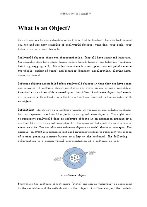
What Is an Object?Objects are key to understanding object-oriented technology. You can look around you now and see many examples of real-world objects: your dog, your desk, your television set, your bicycle.Real-world objects share two characteristics: They all have state and behavior. For example, dogs have state (name, color, breed, hungry) and behavior (barking, fetching, wagging tail). Bicycles have state (current gear, current pedal cadence, two wheels, number of gears) and behavior (braking, accelerating, slowing down, changing gears).Software objects are modeled after real-world objects in that they too have state and behavior. A software object maintains its state in one or more variables.A variable is an item of data named by an identifier. A software object implements its behavior with methods. A method is a function (subroutine) associated with an object.Definition:An object is a software bundle of variables and related methods. You can represent real-world objects by using software objects. You might want to represent real-world dogs as software objects in an animation program or a real-world bicycle as a software object in the program that controls an electronic exercise bike. You can also use software objects to model abstract concepts. For example, an event is a common object used in window systems to represent the action of a user pressing a mouse button or a key on the keyboard. The following illustration is a common visual representation of a software object.A software object.Everything the software object knows (state) and can do (behavior) is expressed by the variables and the methods within that object. A software object that modelsyour real-world bicycle would have variables that indicate the bicycle's current state: Its speed is 18 mph, its pedal cadence is 90 rpm, and its current gear is 5th. These variables are formally known as instance variables because they contain the state for a particular bicycle object; in object-oriented terminology, a particular object is called an instance. The following figure illustrates a bicycle modeled as a software object.A bicycle modeled as a softwareobject.In addition to its variables, the software bicycle would also have methods to brake, change the pedal cadence, and change gears. (It would not have a method for changing its speed because the bike's speed is just a side effect of which gear it's in and how fast the rider is pedaling.) These methods are known formally as instance methods because they inspect or change the state of a particular bicycle instance.Object diagrams show that an object's variables make up the center, or nucleus, of the object. Methods surround and hide the object's nucleus from other objects in the program. Packaging an object's variables within the protective custody of its methods is called encapsulation. This conceptual picture of an object —a nucleus of variables packaged within a protective membrane of methods — is an ideal representation of an object and is the ideal that designers of object-oriented systems strive for. However, it's not the whole story.Often, for practical reasons, an object may expose some of its variables or hide some of its methods. In the Java programming language, an object can specify one of four access levels for each of its variables and methods. The access level determines which other objects and classes can access that variable or method. Refer to the Controlling Access to Members of a Class section for details.Encapsulating related variables and methods into a neat software bundle is a simple yet powerful idea that provides two primary benefits to software developers:Modularity:The source code for an object can be written and maintainedindependently of the source code for other objects. Also, an objectcan be easily passed around in the system. You can give your bicycleto someone else, and it will still work.Information-hiding: An object has a public interface that otherobjects can use to communicate with it. The object can maintain privateinformation and methods that can be changed at any time withoutaffecting other objects that depend on it. You don't need to understanda bike's gear mechanism to use it.What Is a Message?A single object alone generally is not very useful. Instead, an object usually appears as a component of a larger program or application that contains many other objects. Through the interaction of these objects, programmers achieve higher-order functionality and more complex behavior. Your bicycle hanging from a hook in the garage is just a bunch of metal and rubber; by itself, it is incapable of any activity; the bicycle is useful only when another object (you) interacts with it (by pedaling).Software objects interact and communicate with each other by sending messages to each other. When object A wants object B to perform one of B's methods, object A sends a message to object B (see the following figure).Objects interact by sending each other messages.Sometimes, the receiving object needs more information so that it knows exactly what to do; for example, when you want to change gears on your bicycle, you have to indicate which gear you want. This information is passed along with the message as parameters.Messages use parameters to pass alongextra information that the objectneeds —in this case, which gear thebicycle should be in.These three parts are enough information for the receiving object to perform the desired method. No other information or context is required.Messages provide two important benefits:An object's behavior is expressed through its methods, so (aside fromdirect variable access) message passing supports all possibleinteractions between objects.Objects don't need to be in the same process or even on the same machineto send messages back and forth and receive messages from each other. What Is a Class?In the real world, you often have many objects of the same kind. For example, your bicycle is just one of many bicycles in the world. Using object-orientedterminology, we say that your bicycle object is an instanceof the class of objects known as bicycles. Bicycles have some state (current gear, current cadence, two wheels) and behavior (change gears, brake) in common. However, each bicycle's state is independent of and can be different from that of other bicycles.When building them, manufacturers take advantage of the fact that bicycles share characteristics, building many bicycles from the same blueprint. It would be very inefficient to produce a new blueprint for every bicycle manufactured.In object-oriented software, it's also possible to have many objects of the same kind that share characteristics: rectangles, employee records, video clips, and so on. Like bicycle manufacturers, you can take advantage of the fact that objects of the same kind are similar and you can create a blueprint for those objects.A software blueprint for objects is called a class (see the following figure).A visual representation of a class.Definition: A class is a blueprint that defines the variables and the methods common to all objects of a certain kind.The class for our bicycle example would declare the instance variables necessary to contain the current gear, the current cadence, and so on for each bicycle object. The class would also declare and provide implementations for the instance methods that allow the rider to change gears, brake, and change the pedaling cadence, as shown in the next figure.The bicycle class.After you've created the bicycle class, you can create any number of bicycleobjects from that class. When you create an instance of a class, the system allocates enough memory for the object and all its instance variables. Each instance gets its own copy of all the instance variables defined in the class, as the next figure shows.MyBike and YourBike are two different instances of the Bike class. Each instance has its own copy of the instance variables defined in the Bike class but has different values for these variables.In addition to instance variables, classes can define class variables. A class wariable contains information that is shared by all instances of the class. For example, suppose that all bicycles had the same number of gears. In this case, defining an instance variable to hold the number of gears is inefficient; each instance would have its own copy of the variable, but the value would be the same for every instance. In such situations, you can define a class variable that contains the number of gears (see the following figure); all instances share this variable. If one object changes the variable, it changes for all other objects of that type.YourBike, an instance of Bike, has access to the numberOfGears variable in the Bike class; however, the YourBike instance does not have a copy of this class variable.A class can also declare class methods You can invoke a class method directly from the class, whereas you must invoke instance methods on a particular instance.The Understanding Instance and Class Members section discusses instance variables and methods and class variables and methods in detail.Objects provide the benefit of modularity and information-hiding. Classes provide the benefit of reusability. Bicycle manufacturers use the same blueprint over and over again to build lots of bicycles. Software programmers use the same class, and thus the same code, over and over again to create many objects.Objects versus ClassesYou've probably noticed that the illustrations of objects and classes look very similar. And indeed, the difference between classes and objects is often the source of some confusion. In the real world, it's obvious that classes are not themselves the objects they describe; that is, a blueprint of a bicycle is not a bicycle. However, it's a little more difficult to differentiate classes and objects in software. This is partially because software objects are merelyelectronic models of real-world objects or abstract concepts in the first place. But it's also because the term object is sometimes used to refer to both classes and instances.In illustrations such as the top part of the preceding figure, the class is not shaded because it represents a blueprint of an object rather than the object itself. In comparison, an object is shaded, indicating that the object exists and that you can use it.What Is Inheritance?Generally speaking, objects are defined in terms of classes. You know a lot about an object by knowing its class. Even if you don't know what a penny-farthing is, if I told you it was a bicycle, you would know that it had two wheels, handlebars, and pedals.Object-oriented systems take this a step further and allow classes to be defined in terms of other classes. For example, mountain bikes, road bikes, and tandems are all types of bicycles. In object-oriented terminology, mountain bikes, road bikes, and tandems are all subclasses of the bicycle class. Similarly, the bicycle class is the supclasses of mountain bikes, road bikes, and tandems. This relationship is shown in the following figure.The hierarchy of bicycle classes.Each subclass inherits state (in the form of variable declarations) from the superclass. Mountain bikes, road bikes, and tandems share some states: cadence, speed, and the like. Also, each subclass inherits methods from the superclass. Mountain bikes, road bikes, and tandems share some behaviors — braking and changing pedaling speed, for example.However, subclasses are not limited to the states and behaviors provided to them by their superclass. Subclasses can add variables and methods to the ones they inherit from the superclass. Tandem bicycles have two seats and two sets of handlebars; some mountain bikes have an additional chain ring, giving them a lower gear ratio.Subclasses can also override inherited methods and provide specialized implementations for those methods. For example, if you had a mountain bike with an additional chain ring, you could override the "change gears" method so that the rider could shift into those lower gears.You are not limited to just one layer of inheritance. The inheritance tree, or class hierardry, can be as deep as needed. Methods and variables are inherited down through the levels. In general, the farther down in the hierarchy a class appears, the more specialized its behavior.Note:Class hierarchies should reflect what the classes are, not how they're implemented. When implementing a tricycle class, it might be convenient to make it a subclass of the bicycle class —after all, both tricycles and bicycles have a current speed and cadence. However, because a tricycle is not a bicycle, it's unwise to publicly tie the two classes together. It could confuse users, make the tricycle class have methods (for example, to change gears) that it doesn't need, and make updating or improving the tricycle class difficult.The Object class is at the top of class hierarchy, and each class is its descendant (directly or indirectly). A variable of type Object can hold a reference to any object, such as an instance of a class or an array. Object provides behaviors that are shared by all objects running in the Java Virtual Machine. For example, all classes inherit Object's toString method, which returns a string representation of the object. The Managing Inheritance section covers the Object class in detail.Inheritance offers the following benefits:Subclasses provide specialized behaviors from the basis of commonelements provided by the superclass. Through the use of inheritance,programmers can reuse the code in the superclass many times.Programmers can implement superclasses called abstract classes thatdefine common behaviors. The abstract superclass defines and maypartially implement the behavior, but much of the class is undefinedand unimplemented. Other programmers fill in the details withspecialized subclasses.What Is an Interface?In general, an interface is a device or a system that unrelated entities use to interact. According to this definition, a remote control is an interface between you and a television set, the English language is an interface between two people, and the protocol of behavior enforced in the military is the interface between individuals of different ranks.Within the Java programming language, an interface is a type, just as a class is a type. Like a class, an interface defines methods. Unlike a class, an interface never implements methods; instead, classes that implement the interface implement the methods defined by the interface. A class can implement multiple interfaces.The bicycle class and its class hierarchy define what a bicycle can and cannot do in terms of its "bicycleness." But bicycles interact with the world on other terms. For example, a bicycle in a store could be managed by an inventory program. An inventory program doesn't care what class of items it manages as long as each item provides certain information, such as price and tracking number. Instead of forcing class relationships on otherwise unrelated items, the inventory program sets up a communication protocol. This protocol comes in the form of a set of method definitions contained within an interface. The inventory interface would define, but not implement, methods that set and get the retail price, assign a tracking number, and so on.计算机专业中英文文献翻译To work in the inventory program, the bicycle class must agree to this protocol by implementing the interface. When a class implements an interface, the class agrees to implement all the methods defined in the interface. Thus, the bicycle class would provide the implementations for the methods that set and get retail price, assign a tracking number, and so on.You use an interface to define a protocol of behavior that can be implemented by any class anywhere in the class hierarchy. Interfaces are useful for the following:Capturing similarities among unrelated classes without artificiallyforcing a class relationshipDeclaring methods that one or more classes are expected to implementRevealing an object's programming interface without revealing itsclassModeling multiple inheritance, a feature of some object-orientedlanguages that allows a class to have more than one superclass。
计算机专业课程名称英文翻译

计算机专业课程名称英文翻译(计算机科学与技术(教师教育)专业的课程名称和英文名称)4 中国现代史纲要 Outline of Moderm Chinese History5 大学英语 College English6 大学体育 College PE7 心理学 Psychology8 教育学 Pedagogy9 现代教育技术 Modern Technology10 教师口语 Teachers' Oral Skill11 形势与政策 Current Situation and Policy12 大学生就业与指导 Career Guidance13 学科教学法 Course Teaching Methodology14 生理与心理健康教育 Health and Physiology Education15 环境与可持续发展 Environment and Sustainable Development16 文献检索 Literature Retrieval17 大学体育 College PE18 大学语文 College Chinese19 高等数学 Higher Mathematics20 计算机导论 Introduction to ComputerScience21 程序设计基础 Programming Foundations22 程序设计基础实验 Experimentationof ProgrammingFoundations23 线性代数 Linear Algebra24 大学物理 College Physics25 大学物理实验 Experimentation of CollegePhysics26 电路与电子技术 Circuits and Electronics27 电工与电子技术实验 Experimentation of Circuits andElectronics28 数字逻辑电路 Digital Logic Circuit29 数字逻辑电路 Experimentation of DigitalLogic Circuit30 离散数学 Discrete Mathematics31 数据结构 Data Structures32 数据结构实验 Experimentation of DataStructures33 计算机组成与系统结构 Computer Organization and Architecture34 操作系统 Operating System35 操作系统实验 Experimentation of Operating System36 计算机网络 Computer Network37 计算机网络实验 Experimentation of Computer Network38 面向对象程序设计 Object-Oriented Programming39 面向对象程序设计实验 Experimentation of Object-Oriented Programming40 汇编语言程序设计 Assembly Language41 汇编语言程序设计实验 Experimentation of Assembly Language42 概率与数理统计 Probability and Statistics43 JAVA语言 Java Language45 JAVA语言实验 Experimentation of Java Language46 数据库原理 Databases Principles47 数据库原理实验 Experimentation of Databases Pninciples48 专业英语 Discipline English49 人工智能导论 Introduction to Artificial Intelligence50 算法设计与分析 Design and Analysis Of Algorithms51 微机系统与接口 Microcomputer System and Interface52 编译原理 Compiling Principles53 编译原理实验 Experimentation of Compiling54 数学建模 Mathematics Modeling55 软件工程 Software Engineering计算机专业课程名称英文翻译下(2)(计算机科学与技术(教师教育)专业的课程名称和英文名称)56 软件工程实验 Experimentation of Software Engineering57 嵌入式系统 Embedded System58 嵌入式系统实验 Experimentation of Embedded System59 多媒体技术 Multimedia Technology60 Experimentation of Multimedia Technology61 信息系统分析与设计 Object-Oriented Analysis and Design62 UNIX操作系统分析 UNIX System Analysis63 UNIX/Linux操作系统分析Experimentation of UNIX/Linux SystemAnalysis64 单片机原理 Principles of Single-ChipComputer65 信息安全与保密概论Introduction to Security andm Cryptography66 Web应用技术 Applications of Web67 高级数据库应用技术Advanced Application of Database Technology68 组网技术 Technology ofBuildingNetwork69 组网技术实验 Technology of Building Network70 计算机图形学 Computer Graphics71 嵌入式接口技术 Embedded Interface72 嵌入式接口技术实验Experimentation ofEmbedded Interface73 数字图像处理 Digital Images Processing74 数字图像处理实验 Digital Images Processing75 网络应用软件开发 Network Application Development76 XML原理与应用 XML Principle and Application77 XML原理与应用实验 ExperimentationofXML Principle andApplication78 计算机系统维护 Maintenance of Computer System79 计算机系统维护实验 Experimentation ofComputer Maintenance80 网络管理技术 Network Management Technology81 网络管理技术实验Experimentation of NetworkManagement82 数据仓库与数据挖掘 Data Storage and Data Digging83 项目管理 Project Management84 软件开发实例 Cases of Sotiware Development85 企业资源规划( ERP) Enterprise Resource Planning86 新技术 New Technology87 科研创作指导Supervision in Science ResearchCreation88 电子商务概论 Introduction of ElectronicBusiness89 计算机辅助教学 Computer Aided Teaching另:计算机导论 Introduction to ComputerScience程序设计基础 Foundations ofProgramming电路与电子技术 Circuits and Electronics数字逻辑电路 Digital Logic Circuit离散数学 Discrete Mathematics数据结构 Data Structures计算机组成与系统结构 Computer Organization and Architecture操作系统 Operating System计算机网络 Computer Network面向对象程序设计 Object-Oriented Progjamming数据库原理 Databases Principles。
数值计算04-插值与拟合

二维插值的定义
第一种(网格节点):
y
O
x
已知 mn个节点 其中 互不相同,不妨设
构造一个二元函数
通过全部已知节点,即
再用
计算插值,即
第二种(散乱节点):
y
0
x
已知n个节点
其中 互不相同,
构造一个二元函数
通过全部已知节点,即
再用
计算插值,即
最邻近插值
y
( x1 , y2 ) ( x2 , y2 )
( x1 , y1 ) ( x2 , y1 )
x
O
注意:最邻近插值一般不连续。具有连续性的最简单 的插值是分片线性插值。
分片线性插值
速度最快,但平滑性差
linear
占有的内存较邻近点插值方法多,运算时间 也稍长,与邻近点插值不同,其结果是连续 的,但在顶点处的斜率会改变 运算时间长,但内存的占有较立方插值方法 要少,三次样条插值的平滑性很好,但如果 输入的数据不一致或数据点过近,可能出现 很差的插值结果 需要较多的内存和运算时间,平滑性很好 二维插值函数独有。插值点处的值和该点值 的导数都连续
x=0 0.5 1 1.5 2 2.5 3 3.5 4 4.5 5 y=0 0.5 1 1.5 2 2.5 3 3.5 4 4.5 5 5.5 6
海拔高度数据为: z=89 90 87 85 92 91 96 93 90 87 82 92 96 98 99 95 91 89 86 84 82 84 96 98 95 92 90 88 85 84 83 81 85 80 81 82 89 95 96 93 92 89 86 86 82 85 87 98 99 96 97 88 85 82 83 82 85 89 94 95 93 92 91 86 84 88 88 92 93 94 95 89 87 86 83 81 92 92 96 97 98 96 93 95 84 82 81 84 85 85 81 82 80 80 81 85 90 93 95 84 86 81 98 99 98 97 96 95 84 87 80 81 85 82 83 84 87 90 95 86 88 80 82 81 84 85 86 83 82 81 80 82 87 88 89 98 99 97 96 98 94 92 87
插值和拟合

插值和拟合都是函数逼近或者数值逼近的重要组成部分他们的共同点都是通过已知一些离散点集M上的约束,求取一个定义在连续集合S(M包含于S)的未知连续函数,从而达到获取整体规律的目的,即通过"窥几斑"来达到"知全豹"。
简单的讲,所谓拟合是指已知某函数的若干离散函数值{f1,f2,…,fn},通过调整该函数中若干待定系数f(λ1, λ2,…,λ3), 使得该函数与已知点集的差别(最小二乘意义)最小。
如果待定函数是线性,就叫线性拟合或者线性回归(主要在统计中),否则叫作非线性拟合或者非线性回归。
表达式也可以是分段函数,这种情况下叫作样条拟合。
而插值是指已知某函数的在若干离散点上的函数值或者导数信息,通过求解该函数中待定形式的插值函数以及待定系数,使得该函数在给定离散点上满足约束。
插值函数又叫作基函数,如果该基函数定义在整个定义域上,叫作全域基,否则叫作分域基。
如果约束条件中只有函数值的约束,叫作Lagrange插值,否则叫作Hermite插值。
从几何意义上将,拟合是给定了空间中的一些点,找到一个已知形式未知参数的连续曲面来最大限度地逼近这些点;而插值是找到一个(或几个分片光滑的)连续曲面来穿过这些点。
一、概念的引入1. 插值与拟合在现实生活中的应用l 机械制造:汽车外观设计l 采样数据的重新建构:电脑游戏中场景的显示,地质勘探,医学领域(CT)2.概念的定义l 插值:基于[a,b]区间上的n个互异点,给定函数f(x),寻找某个函数去逼近f(x)。
若要求φ(x)在xi处与f(xi)相等,这类的函数逼近问题称为插值问题,xi即是插值点l 逼近:当取值点过多时,构造通过所有点的难度非常大。
此时选择一个次数较低的函数最佳逼近这些点,一般采用最小二乘法l 光顾:曲线的拐点不能太多,条件:①二阶几何连续②不存在多余拐点③曲率变化较小l 拟合:曲线设计过程中用插值或通过逼近方法是生成的曲线光滑(切变量连续)光顾二、插值理论设函数y=f(x)在区间[a,b]上连续,在[a,b]上有互异点x0,x1,…,xn处取值y 0,y1,…,yn。
毕业设计论文外文文献翻译计算机科学与技术微软VisualStudio中英文对照

外文文献翻译(2012届)学生姓名学号********专业班级计算机科学与技术08-5班指导教师微软Visual Studio1微软Visual StudioVisual Studio 是微软公司推出的开发环境,Visual Studio可以用来创建Windows平台下的Windows应用程序和网络应用程序,也可以用来创建网络服务、智能设备应用程序和Office 插件。
Visual Studio是一个来自微软的集成开发环境IDE(inteqrated development environment),它可以用来开发由微软视窗,视窗手机,Windows CE、.NET框架、.NET精简框架和微软的Silverlight支持的控制台和图形用户界面的应用程序以及Windows窗体应用程序,网站,Web应用程序和网络服务中的本地代码连同托管代码。
Visual Studio包含一个由智能感知和代码重构支持的代码编辑器。
集成的调试工作既作为一个源代码级调试器又可以作为一台机器级调试器。
其他内置工具包括一个窗体设计的GUI应用程序,网页设计师,类设计师,数据库架构设计师。
它有几乎各个层面的插件增强功能,包括增加对支持源代码控制系统(如Subversion和Visual SourceSafe)并添加新的工具集设计和可视化编辑器,如特定于域的语言或用于其他方面的软件开发生命周期的工具(例如Team Foundation Server的客户端:团队资源管理器)。
Visual Studio支持不同的编程语言的服务方式的语言,它允许代码编辑器和调试器(在不同程度上)支持几乎所有的编程语言,提供了一个语言特定服务的存在。
内置的语言中包括C/C + +中(通过Visual C++),(通过Visual ),C#中(通过Visual C#)和F#(作为Visual Studio 2010),为支持其他语言,如M,Python,和Ruby等,可通过安装单独的语言服务。
计算机专业中英文翻译外文翻译文献翻译
英文参考文献及翻译Linux - Operating system of cybertimes Though for a lot of people , regard Linux as the main operating system to make up huge work station group, finish special effects of " Titanic " make , already can be regarded as and show talent fully. But for Linux, this only numerous news one of. Recently, the manufacturers concerned have announced that support the news of Linux to increase day by day, users' enthusiasm to Linux runs high unprecedentedly too. Then, Linux only have operating system not free more than on earth on 7 year this piece what glamour, get the favors of such numerous important software and hardware manufacturers as the masses of users and Orac le , Informix , HP , Sybase , Corel , Intel , Netscape , Dell ,etc. , OK?1.The background of Linux and characteristicLinux is a kind of " free (Free ) software ": What is called free,mean users can obtain the procedure and source code freely , and can use them freely , including revise or copy etc.. It is a result of cybertimes, numerous technical staff finish its research and development together through Inte rnet, countless user is it test and except fault , can add user expansion function that oneself make conveniently to participate in. As the most outstanding one in free software, Linux has characteristic of the following:(1)Totally follow POSLX standard, expand the network operatingsystem of supporting all AT&T and BSD Unix characteristic. Because of inheritting Unix outstanding design philosophy , and there are clean , stalwart , high-efficient and steady kernels, their all key codes are finished by Li nus Torvalds and other outstanding programmers, without any Unix code of AT&T or Berkeley, so Linu x is not Unix, but Linux and Unix are totally compatible.(2)Real many tasks, multi-user's system, the built-in networksupports, can be with such seamless links as NetWare , Windows NT , OS/2 ,Unix ,etc.. Network in various kinds of Unix it tests to be fastest in comparing and assess efficiency. Support such many kinds of files systems as FAT16 , FAT32 , NTFS , Ex t2FS , ISO9600 ,etc. at the same time .(3) Can operate it in many kinds of hardwares platform , including such processors as Alpha , SunSparc , PowerPC , MIPS ,etc., to various kinds of new-type peripheral hardwares, can from distribute on global numerous programmer there getting support rapidly too.(4) To that the hardware requires lower, can obtain very good performance on more low-grade machine , what deserves particular mention is Linux outstanding stability , permitted " year " count often its running times.2.Main application of Linux At present,Now, the application of Linux mainly includes:(1) Internet/Intranet: This is one that Linux was used most at present, it can offer and include Web server , all such Inter net services as Ftp server , Gopher server , SMTP/POP3 mail server , Proxy/Cache server , DNS server ,etc.. Linux kernel supports IPalias , PPP and IPtunneling, these functions can be used for setting up fictitious host computer , fictitious service , VPN (fictitious special-purpose network ) ,etc.. Operating Apache Web server on Linux mainly, the occupation rate of market in 1998 is 49%, far exceeds the sum of such several big companies as Microsoft , Netscape ,etc..(2) Because Linux has outstanding networking ability , it can be usedin calculating distributedly large-scaly, for instance cartoon making , scientific caculation , database and file server ,etc..(3) As realization that is can under low platform fullness of Unix that operate , apply at all levels teaching and research work of universities and colleges extensively, if Mexico government announce middle and primary schools in the whole country dispose Linux and offer Internet service for student already.(4) Tabletop and handling official business appliedly. Application number of people of in this respect at present not so good as Windows of Microsoft far also, reason its lie in Lin ux quantity , desk-top of application software not so good as Windows application far not merely, because the characteristic of the freedom software makes it not almost have advertisement thatsupport (though the function of Star Office is not second to MS Office at the same time, but there are actually few people knowing).3.Can Linux become a kind of major operating system?In the face of the pressure of coming from users that is strengthened day by day, more and more commercial companies transplant its application to Linux platform, comparatively important incident was as follows, in 1998 ①Compaq and HP determine to put forward user of requirement truss up Linux at their servers , IBM and Dell promise to offer customized Linux system to user too. ②Lotus announce, Notes the next edition include one special-purpose edition in Linux. ③Corel Company transplants its famous WordPerfect to on Linux, and free issue. Corel also plans to move the other figure pattern process products to Linux platform completely.④Main database producer: Sybase , Informix , Oracle , CA , IBM have already been transplanted one's own database products to on Linux, or has finished Beta edition, among them Oracle and Informix also offer technical support to their products.4.The gratifying one is, some farsighted domestic corporations have begun to try hard to change this kind of current situation already. Stone Co. not long ago is it invest a huge sum of money to claim , regard Linux as platform develop a Internet/Intranet solution, regard this as the core and launch Stone's system integration business , plan to set up nationwide Linux technical support organization at the same time , take the lead to promote the freedom software application and development in China. In addition domestic computer Company , person who win of China , devoted to Linux relevant software and hardware application of system popularize too. Is it to intensification that Linux know , will have more and more enterprises accede to the ranks that Linux will be used with domestic every enterprise to believe, more software will be planted in Linux platform. Meanwhile, the domestic university should regard Linux as the original version and upgrade already existing Unix content of courses , start with analysing the source code and revising the kernel and train a large number of senior Linux talents, improve our country's own operating system. Having only really grasped the operating system, the software industry of our country could be got rid of and aped sedulously at present, the passive state led by the nose by others, create conditions for revitalizing the software industry of our country fundamentally.中文翻译Linux—网络时代的操作系统虽然对许多人来说,以Linux作为主要的操作系统组成庞大的工作站群,完成了《泰坦尼克号》的特技制作,已经算是出尽了风头。
quadratic_interpolation_method_概述及解释说明

quadratic interpolation method 概述及解释说明1. 引言1.1 概述在数学和计算机科学领域中,quadratic interpolation method(二次插值法)是一种通过已知的数据点来估算未知数据点的方法。
它是在给定三个已知数据点之间构建一个二次方程,并使用该方程来预测其他位置的数值。
1.2 文章结构本文将首先介绍quadratic interpolation method的定义和原理,然后探讨它在实际应用中的优势和限制。
最后,我们将总结文章并得出结论。
1.3 目的本文的目的是向读者介绍quadratic interpolation method这一重要的插值方法。
通过了解其定义、原理以及实际应用中所面临的挑战,读者可以更好地理解二次插值法在解决实际问题中的作用和局限性。
期待您在撰写文章过程中能够充分展示quadratic interpolation method这一主题,并为读者提供足够清晰和详细的信息。
2. 正文在数学和计算机科学领域,插值是一种通过已知数据点推断未知数据点的方法。
其中,二次插值方法是一种常用且有效的插值技术,奠定了许多其他高级插值算法的基础。
二次插值方法主要基于二次多项式函数,在已知三个数据点的情况下,通过构造一个二次多项式来逼近这些数据点之间的曲线。
这里所说的二次多项式是指具有二次阶数(degree)的多项式,其表达形式为:```f(x) = ax^2 + bx + c```其中,a、b和c是未知系数。
为了通过这些系数来确定唯一的二次函数,需要求解一个包含三个等式的方程组。
具体而言,给定三个已知数据点`(x1, y1)`、`(x2, y2)` 和`(x3, y3)` ,根据这些数据点构建以下方程组:```y1 = a*x1^2 + b*x1 + cy2 = a*x2^2 + b*x2 + cy3 = a*x3^2 + b*x3 + c```利用这个方程组,可以求解出未知系数`a`、`b` 和`c` 的值,并得到由这些系数确定的二次函数。
数值分析中的插值与拟合

数值分析中的插值与拟合插值和拟合是数值分析中常用的技术,用于估计或预测数据集中缺失或未知部分的数值。
在本文中,我们将讨论插值和拟合的概念、方法和应用。
一、插值插值是通过已知数据点之间的连续函数来估计中间数据点的数值。
插值方法可以根据不同的数据和需求选择合适的插值函数,常用的插值方法包括拉格朗日插值、牛顿插值和埃尔米特插值。
1.1 拉格朗日插值拉格朗日插值是一种基于多项式的插值方法。
通过已知的n个数据点,可以构建一个n-1次的插值多项式。
这个多项式通过已知数据点上的函数值来准确地经过每一个点。
1.2 牛顿插值牛顿插值方法也是一种多项式插值方法,通过差商的概念来构建插值多项式。
差商是一个递归定义的系数,通过已知数据点的函数值计算得出。
牛顿插值可以通过递推的方式计算出插值多项式。
1.3 埃尔米特插值埃尔米特插值是一种插值方法,适用于已知数据点和导数值的情况。
它基于拉格朗日插值的思想,通过引入导数信息来逼近数据的真实分布。
埃尔米特插值可以更准确地估计数据点之间的值,并且可以保持导数的连续性。
二、拟合拟合是通过一个模型函数来逼近已知数据点的数值。
拟合方法旨在找到最适合数据集的函数形式,并通过最小化误差来确定函数的参数。
常见的拟合方法包括最小二乘法、多项式拟合和曲线拟合。
2.1 最小二乘法最小二乘法是一种常用的拟合方法,通过最小化数据点到拟合函数的误差平方和来确定最佳拟合曲线或曲面。
最小二乘法适用于线性和非线性拟合问题,可以用于拟合各种类型的非线性函数。
2.2 多项式拟合多项式拟合是一种基于多项式函数的拟合方法。
通过多项式的线性组合来近似已知数据集的数值。
多项式拟合可以通过最小二乘法或其他优化算法来确定拟合函数的系数。
2.3 曲线拟合曲线拟合是一种用曲线函数来逼近已知数据点的拟合方法。
曲线函数可以是非线性的,并且可以根据数据的特点进行选择。
曲线拟合可以通过优化算法来确定拟合函数的参数。
三、应用插值和拟合在数值分析中有广泛的应用。
计算机科学与技术专业外文翻译--计算机与制造业

外文原文:The Computer and ManufacturingThe computer is bringing manufactuing into the Information Age.This new tool, long a familiar one in business and management operation, is moving into the factory, and its advent is changing manufacturing as certainly as the stean engine changed it more than 200 years ago.The basic metalworking processes are not likely to change fundamentally, but their organization and contral definitely will.In one respect , manufacturing could be said to be coming full circle. The first manufacturing was a cottage industry: the designer was also the manufacturer, conceiving and fabricating products one at a time.Eventually,the concept of the interchangeability of parts was developed, producted thousanda at a time.Today , although the designer and manufacturer may not become one again, the functions are being drawn close in the movement toward an integrated manufacturing system.It ia perhaps ironic that, at a time when the market demands a hinh degree of product diversification, the manufacturing enteprises have to increase productivity and reduce costs, Customers are demanding hinh quality and diversified products for less money.The computer is the key to meet these requirements. It is the only tool that can provide the quick reflexes, the flexibility and speed, to meet a diversified market. And it is the only tool that enables the detailed analysis and the accesssibilty of accurate data necessary for the integration of the manufacturing system.It may well be that, in the future, the computer may be essential to a company’s survival. Many of today’s businesses will fade away tobe replaced by more-productive combinations. Such more-productive combinations are superquality, superproductivity plants. The goal is to design and operate a plant that would produce 100% satisfactory parts with good productivity.A sophisticated, competitive world is requiring that manufacturing begin to settle for more, to become itself sophisticated. To meet competition, for example, acompany will have to meet the somewhat conflicting demands for greater product diversification, hinher quality, improved productivity, and low prices.The company that seeks to meet these demands will need a sophisticated tool, one that will allow it to respond quickly to customer needs while getting the most out of its manufacturing resources.The computer is that tool.Becoming a “superquality, superproductivity” plant requires the integration of an extremely complex system. This can be accomplished only when all elements of manufacturing-design, fabrication and assembly, quality assurance, management, materials handling-are computer integrated.In product design, for example, interactive computer-aided-design(CAD) systems allow the drawing and analysis tasks to be performed in a fraction of the time previously required and with greater accuracy. And programs for prototype testing and evaluation further speed the design process.In manufacturing planning, computer-aided process planning permits the selection, from thousands of possible sequences and schedules, of the optinun process.On the shop floor, distributed intelligence in the form of microprocessors controls machines, runs automated loading and unloading equipment, and collects data on current shop conditions.But such isolated revolutions are not enough, What is needed is a totally automated system, linked by common software from front door to back..Essentially,computer integration provides widely and instantaneously available, accurate information, improving communication between departments, permitting tighter control, and generally enhancing the overall quality and efficiency of the entire system.Improved communication can mean, for example, designs that are more producible. The NC programmer and the tool designer have a chance to influence the product designer,and vice versa.Engineering changes, thus, can be reduced, and those that are required can be handled more efficiently. Not only does the computer permit them to be specified more quickly, but it also alerts subsequent users of the data to the fact that a change has been made.The instantaneous updating of production-control data permits better planning and more-effective scheduling. Expensive equipment, therefore, is used moreproductively, and parts move more efficiently through production, reducing work-in-process costs.Product quality, too, can be improved. Not only are more-accurate designs produced, for example, but the use of design data by the quality-assurance department helps eliminate errors due to misunderstandings.People are enabled to do sheir jobs better. By eliminating tedious calculation and paperwork-not to mention time wasted searching for information-the computer mot only allows workers to be more productive but also frees them to do what only human beings can do :think creatively.Computer integration may also lure new people into manufacturing. People are attracted because they want to work in a modern, technologically sophisticated environment.In manufacturing engineering, CAD/CAM decreases tool-design, NC-programming, and planning times while speeding the response rate, which eill eventually permit in-house staff to perform work that is currently being contracted out.中文译文:计算机与制造业计算机正在将制造业带入信息时代。
- 1、下载文档前请自行甄别文档内容的完整性,平台不提供额外的编辑、内容补充、找答案等附加服务。
- 2、"仅部分预览"的文档,不可在线预览部分如存在完整性等问题,可反馈申请退款(可完整预览的文档不适用该条件!)。
- 3、如文档侵犯您的权益,请联系客服反馈,我们会尽快为您处理(人工客服工作时间:9:00-18:30)。
外文原文:PADE APPROXIMATION BY RATIONAL FUNCTION 129We can apply this formula to get the polynomial approximation directly for a given function f (x), without having to resort to the Lagrange or Newtonpolynomial. Given a function, the degree of the approximate polynomial, and the left/right boundary points of the interval, the above MATLAB routine “cheby()” uses this formula to make the Chebyshev polynomial approximation.The following example illustrates that this formula gives the same approximate polynomial function as could be obtained by applying the Newton polynomial with the Chebyshev nodes.Example 3.1. Approximation by Chebyshev Polynomial. Consider the problem of finding the second-degree (N = 2) polynomial to approximate the function 2()1/(18)f x x =+. We make the following program “do_cheby.m ”, which uses the MATLAB routine “cheby()” for this job and uses Lagrange/Newton polynomial with the Chebyshev nodes to do the same job. Readers can run this programto check if the results are the same.3.4 PADE APPROXIMATION BY RATIONAL FUNCTIONPade approximation tries to approximate a function f (x) around a point xo by a rational function00,00020012002012()()()()()()1()()()M M N N M M N N Q x x p x x D x x q q x x q x x q x x d x x d x x x x --=-+-+--+-+-+-++=+d (3.4.1)where 00(2)0()0(),'(),(),,()M N f x f x f x f x + are known.How do we find such a rational function? We write the Taylor series expansion of f (x) up to degree M + N at x = xo as130 INTERPOLATION AND CURVE FITTING(2)0()000000200020012()()()()()'()()()()2()!()()()(3.4.2)M N M NM N M N M N f x f x f x T x x f x f x x x x x x x M N a a x x a x x a x x +++++≈-=+-+-++-+=+-+-++- Assuming 0x =0for simplicity, we get the coefficients of ()()N M D x andQ x such that()()0()M M N N Q x T x D x +-=011011()(1)()01M N N N M N N N N N a a x a x d x d x q q x q x d x d x ++++++++-+++=+++01101()(1)()M N N N M N N N a a x a x d x d x q q x q x ++++++++=+++ (3.4.3) by solving the following equations:0010112110221122111212112212000M M M M N N M M M M M N N M M M M N N M N M N M N M N a q a a d q a a d a d q a a d a d a d q a a d a d a d a a d a d a d a a d a d a d ---+--+++-++++=⎧⎪+=⎪⎪+=⎪⎪⎪⎨⎪=⎪+=⎪⎪⎪⎪=⎩++++++++++++(3.4.4a )(3.4.4b ) Here, we must first solve Eq. (3.4.4b) for N d d d ,,,21 and then substitute di ’sinto Eq. (3.4.4a) to obtain M q q q ,,,10The MATLAB routine “padeap()” implements this scheme to find the coefficient vectors of the numerator/denominator polynomial )(/)(x D x Q N M of thePade approximation for a given function f (x). Note the following things:ž The derivatives (2)()000'(),(),,()M N f x f x f x + up to order (M + N ) arecomputed numerically by using the routine “difapx()”, that will be introduced in Section 5.3.ž In order to compute the values of the Pade approximate function, we substitute 0x x - for x in ,()M N p x which has been obtained with the assumptionthat 0x =0.PADE APPROXIMATION BY RATIONAL FUNCTION 131Example 3.2. Pade Approximation for ()x f x e = . Let’s find the Padeapproximation3,232()()/()p x Q x D x = for ()x f x e = around 0x =0. We make theMATLAB program “do_pade.m ”, which uses the routine “padeap()” for thisjob and uses it again with no output argument to see the graphic results as depicted in Fig. 3.6.To confirm and support this result from the analytical point of view and to help the readers understand the internal mechanism, we perform the hand-calculation 132 INTERPOLATION AND CURVE FITTINGFigure 3.6 Pade approximation and Taylor series expansion for f(x) = ex(Example 3.2.).procedure. First, we write the Taylor series expansion at x = 0 up to degreeM + N = 5 for the given function ()xasf x e()230()11()1!23!K M Nk y k f x T x x x x x k +===++++∑ (E3.2.1) whose coefficients are0123111,1,,,26a a a a ==== (E3.2.2)We put this into Eq. (3.4.4b) with M = 3,N = 2 and solve it for di ’s to get2212431223211211221()10,02/51/61/21/24,/201/241/61/120D x d x d x a a d a d a a d a d d d d d a =++++=++=--⎡⎤⎡⎤⎡⎤⎡⎤⎡⎤==⎢⎥⎢⎥⎢⎥⎢⎥⎢⎥-⎣⎦⎣⎦⎣⎦⎣⎦⎣⎦ (E3.2.3)Substituting this to Eq. (3.4.4a) yields001101221102332112111(2/5)3/51/21(2/5)1(1/20)3/201/6(1/2)(2/5)1(1/20)1/60q a q a a d q a a d a d q a a d a d ===+=+⨯-==++=+⨯-+⨯==++=+⨯-+⨯= (E3.2.4) INTERPOLATION BY CUBIC SPLINE 133 With these coefficients, we write the Pade approximate function as2333,222322()1(3/5)(3/20)(1/60)()()1(2/5)(1/20)(1/3)31220820Q x x x x p x D x x x x x x x x +++===+-++++-+ (E3.2.5)3.5 INTERPOLATION BY CUBIC SPLINEIf we use the Lagrange/Newton polynomial to interpolate a given set of N + 1data points, the polynomial is usually of degree N and so has N − 1 local extrema (maxima/minima). Thus, it will show a wild swing/oscillation (called ‘polynomial wiggle’), particularly near the ends of the whole interval as the number of datapoints increases and so the degree of the polynomial gets higher, as illustratedin Fig. 3.2. Then, how about a piecewise-linear approach, like assigning theindividual approximate polynomial to every subinterval between data points?How about just a linear interpolation —that is, connecting the data points bya straight line? It is so simple, but too short of smoothness. Even with thesecond-degree polynomial, the piecewise-quadratic curve is not smooth enoughto please our eyes, since the second-order derivatives of quadratic polynomials for ad jacent subintervals can’t be made to conform with each other. In real life, there are many cases where the continuity of second-order derivatives isdesirable. For example, it is very important to ensure the smoothness up to order 2 for interpolation needed in CAD (computer-aided design)/CAM (computer-aided manufacturing), computer graphic, and robot path/trajectory planning. That’s why we often resort to the piecewise-cubic curve constructed by the individual thirddegree polynomials assigned to each subinterval, which is called the cubic splineinterpolation. (A spline is a kind of template that architects use to draw a smooth curve between two points.)For a given set of data points {(,),0:}k k x y k N =, the cubic spline s(x)consists of N cubic polynomial ()k s x ’s assigned to each subinterval satisfying the following constraints (S0)–(S4).(S0)32,3,2,1,01()()()()(),[,],0:k k k k k k k k k k s x s x S x x S x x S x x S x x x k N +==-+-+-+∈=for (S1),0()0:k k k k s x S y k N ===,for(S2)1,0()(),1:1k k k k k k s x s x S y k N -≡===-for(S3)1,1'()'(),1:1k k k k k s x s x S k N -≡==-for(S4)1,2''()''()2,1:1k k k k k s x s x S k N -≡==-forThese constraints (S1)–(S4) amount to a set of N + 1 + 3(N − 1) = 4N − 2linear equations having 4N coefficients of the N cubic polynomials,0,1,2,3{,,,,0:1}k k k k S S S S k N =-134 INTERPOLATION AND CURVE FITTINGTable 3.4 Boundary Conditions for a Cubic Splineas their unknowns. Two additional equations necessary for the equations to besolvable are supposed to come from the boundary conditions for the first/secondorder derivatives at the end points (x 0, y 0) and (xN, yN ) as listed in Table 3.4.Now, noting from (S1) that ,0k k S y =, we will arrange the constraints (S2)–(S4)and eliminate Sk,1, Sk,3’s to set up a set of equations with respect to the N + 1 unknowns ,2{,0:}k S k N =. In order to do so, we denote each interval width by 1k k k h x x +=- and substitute (S0) into (S4) to write1,3,2111,2,31,2,2''()62''()21()3k k k k k k k k k k k k s x S h S s x S S h S S +++++=+≡==- (3.5.1a)1,31,21,21()3k k k k S h S S ---=- (3.5.1b) We substitute these equations into (S2) with k + 1 in place of k321,31,21,11,0132,3,2,11()()()()k k k k k k k k k k k k k k k k k k k k k s x S x x S x x S x x S y S h S h S h y y ++++++=-+-+-+≡+++≡to eliminate ,3k S ’s and rewrite it as11,2,2,2,1()3k k k k k k k k k kh y y S S S h S dy h ++--++== 1,2,2,1(2)33k k k k k h S S S dy +++= (3.5.2a ) 1,21,21,11(2)33k k k k k h S S S dy ----++= (3.5.2b ) We also substitute Eq. (3.5.1b) into (S3)211,311,211,1,1'()3k k k k k k k k s x S h S h S S ------=++≡INTERPOLATION BY CUBIC SPLINE 135to write,11,11,21,211,21,21,2()2()k k k k k k k k k k S S h S S h S h S S --------=-+=+ (3.5.3)In order to use this for eliminating Sk,1 from Eq. (3.5.2), we subtract (3.5.2b) from (3.5.2a) to write1,2,21,21,2,11,11(2)(2)3(2)3()k k k k k k k k k k h S S h S S S S dy dy +----+-++-=-and then substitute Eq. (3.5.3) into this to write1,2,21,21,21,21,2111,21,21,21(2)(2)3()3()()3()k k k k k k k k k k k k k k k k k k k k h S S h S S h S S dy dy h S h h S h S dy dy +--------+-+-+++=-+++=- (3.5.4)for k = 1 : N − 1 Since these are N − 1 equations with respect to N + 1 unknowns ,2{,0:}k S k N =, we need two more equations from the boundary conditions to be given aslisted in Table 3.4.How do we convert the boundary condition into equations? In the case where the first-order derivatives on the two boundary points are given as (i) in Table 3.4, we write Eq. (3.5.2a) for k = 0 as01,20,20,1000,201,200,1(2)33,233h S S S dy h S h S dy S ++=+=- (3.5.5a )We also write Eq. (3.5.2b) for k = N as1,21,21,11(2)33N N N N N h S S S dy ----++=and substitute (3.5.3)(k = N ) into this to write01,20,20,10(2)33h S S S dy ++=1,21,21,11,21,2111,21,2,11(2)33(2)323()N N N N N N N N N N N N N N h S S S h S S dy h S h S S dy ----------++-+=+=- (3.5.5b)Equations (3.5.5a) and (3.5.5b) are two additional equations that we need to solve Eq. (3.5.4) and that’s it. In the case where the second -order derivatives on the two boundary points are given as (ii) in Table 3.4, 0,2S and ,2N S are directly known from the boundary conditions as0,200''()/2S s x =,,2''()/2N N N S s x = (3.5.6) 136 INTERPOLATION AND CURVE FITTINGand, subsequently, we have just N − 1 unknowns. In the case where the secondorderderivatives on the two boundary points are given as (iii) in Table 3.4we can instantly convert these into two equations with respect to S 0,2 and SN,2 as Finally, we combine the two equations (3.5.5a) and (3.5.5b) with Eq. (3.5.4) to write it in the matrix –vector form as0,200,1001,21000111,2122211,2,11113()203()2()003()2()3()02N N N N N N N N N N N N S dy S h h S dy dy h h h h S dy dy h h h h S S dy h h -----------⎡⎤⎡⎤⎡⎤⎢⎥⎢⎥⎢⎥-+⎢⎥⎢⎥⎢⎥⎢⎥⎢⎥⎢⎥=⎢⎥⎢⎥⎢⎥-+⎢⎥⎢⎥⎢⎥⎢⎥⎢⎥⎢⎥-⎣⎦⎣⎦⎣⎦ (3.5.8) After solving this system of equation for {Sk,2, k = 0 : N }, we substitute theminto (S1), (3.5.2), and (3.5.1) to get the other coefficients of the cubic spline asThe MATLAB routine “cspline()” constructs Eq.(3.5.8), solves it to get the cubic spline coefficients for given x, y coordinates of the data points and the boundary conditions, uses the mkpp() routine to get the piecewise polynomialexpression, and then uses the ppval() routine to obtain the value(s) of the piecewise polynomial function for xi —that is, the interpolation over xi. The type ofthe boundary condition is supposed to be specified by the third input argument KC. In the case where the boundary condition is given as (i)/(ii) in Table 3.4,the input argument KC should be set to 1/2 and the fourth and fifth input arguments must be the first/second derivatives at the end points. In the case wherethe boundary condition is given as extrapolated like (iii) in Table 3.4, the input argument KC should be set to 3 and the fourth and fifth input arguments do not need to be fed.INTERPOLATION BY CUBIC SPLINE 137(cf) See Problem 1.11 for the usages of the MATLAB routines mkpp() and ppval(). Example 3.3. Cubic Spline. Consider the problem of finding the cubic spline interpolation for the N + 1 = 4 data pointssubject to the boundary condition(E3.3.2)With the subinterval widths on the x-axis and the first divided differences as138INTERPOLATION AND CURVE FITTINGwe write Eq. (3.5.8) as0,200,11,2102,2213,23,113()210033()141063()014163()00123S dy S S dy dy S dy dy S S dy --⎡⎤⎡⎤⎡⎤⎡⎤⎢⎥⎢⎥⎢⎥⎢⎥-⎢⎥⎢⎥⎢⎥⎢⎥==⎢⎥⎢⎥-⎢⎥⎢⎥-⎢⎥⎢⎥⎢⎥⎢⎥-⎣⎦⎣⎦⎣⎦⎣⎦(E3.3.4)Then we solve this equation to get and substitute this into Eq. (3.5.9) to obtain0,01,02,000,102,20,211,112,21,222,123,21,21,20,20,301,21,21,313,22,30,1,4( 3.3.6)(2)2( 3.3.7)3(2)2( 3.3.7)3(2)2( 3.3.7)32( 3.3.8)32( 3.3.8)3S S S E h S dy S S E a hS dy S S E b h S dy S S E c S S S E a h S S S E b h S S ====-+==-+==-+=-==-==--=2,222( 3.3.8)3S E c h =Figure 3.7 Cubic splines for Example 3.3.Finally, we can write the cubic spline equations collectively from (S0) asWe make and run the program “do_csplines.m”, which uses the routine“cspline()” to compute the cubic spline coefficientsand obtain the value(s) of the cubicspline function for i x(i.e., theinterpolation over xi) and then plots the result as depicted in Fig. 3.7. We also compare this result with that obtained by using the MATLAB built-in function “spline(x,y,xi)”, which works with the boundary condition of type (i) for the second input argument given as [dy0 y dyN], and with the boundary conditionof type (iii) for the same lengths of x and y.3.6 HERMITE INTERPOLATING POLYNOMIALIn some cases, we need to find the polynomial function that not only passes through the given points, but also has the specified derivatives at every data point. We call such a polynomial the Hermite interpolating polynomial or the osculating polynomial.140 INTERPOLATION AND CURVE FITTINGFor simplicity, we consider a third-order polynomialmatching just two points and having the specified first derivativesat the points. We can obtain the four coefficients by solvingAs an alternative, we approximate the specified derivatives at the data points by their differencesand find the Lagrange/Newton polynomial matching the four pointsThe MATLAB routine “hermit()” constructs Eq. (3.6.2) and solves it to getthe Hermite interpolating polynomial coefficients for a single interval given thetwo end points and the derivatives at them as the input arguments. The next routine “hermits()” uses “hermit()” to get the Hermite coefficients for a setof multiple subintervals.Example 3.4. Hermite Interpolating Polynomial. Consider the problem of finding the polynomial interpolation for the N + 1 = 4 data pointsTWO-DI MENSIONAL INTERPOLATION 141subject to the conditionsFor this problem, we only have to type the following statements in the MATLAB command window.3.7 TWO-DIMENSIONAL INTERPOLATIONIn this section we deal with only the simplest way of two-dimensional interpolation—that is, a generalization of piecewise linear interpolation calledFigure 3.8 A two-dimensional interpolation using Zi = interp2() on the grid points [Xi,Yi] generated by the meshgrid() command.142 INTERPOLATION AND CURVE FITTINGthe bilinear interpolation. The bilinear interpolation for a point (x, y ) on the rectangularsub-region having and as its left-upper/right-lower corner points is described by the following formula.11111,1111,11,11,11(,)(,)(,)1{()()()()()()()()()()},,n n n n n n n n m n m n m m n n m n m n m n m n m n m n m m n ny y y y z x y z x y z x y y y y y x x y y z x x y y x x y y z x x y y z x x y y z x x x y y y -----------------=+--=----+--+--+--≤≤≤≤for (3.7.2)This formula is cast into the MATLAB routine “intrp2()”, which is so named in order to distinguish it from the MATLAB built-in routine “interp2()”. Note that in reference to Fig. 3.8, the given values of data at grid points (x(m),y(n)) and the interpolated values for intermediate points (xi(m),yi(n)) are stored in Z(n,m) and Zi(n,m), respectively.CURVE FITTING 143Example 3.5. Two-Dimensional Bilinear Interpolation. We consider interpolating the sample values of a functionfor the 5 × 5 grid over the 21 × 21 grid on the domainWe make the MATLA B program “do_interp2.m”, which uses the routine“intrp2()” to do this job, compares its function with that of the MATLABbuilt-in routine “interp2()”, and computes a kind of relative error to estimatehow close the interpolated values are to the original values. The graphic resultsof running this program are depicted in Fig. 3.9, which shows that we obtaineda reasonable approximation with the error of 2.6% from less than 1/16 of the original data. It is implied that the sampling may be a simple data compression method, as long as the interpolated data are little impaired.3.8 CURVE FITTINGWhen many sample data pairs {(xk, yk), k = 0 : M} are available, we often need to grasp the relationship between the two variables or to describe the trend of the(a) True function (b) The function over (c) Bilinear interpolation Figure 3.9 Two-dimensional interpolation (Example 3.5).144 INTERPOLATION AND CURVE FITTINGsample grid data, hopefully in a form of function y = f (x). But, as mentioned in Remark 3.1,the polynomial approach meets with the polynomial wiggle and/or Runge phenomenon,which makes it not attractive for approximation purpose. Although thecubic spline approach may be a roundabout toward the smoothness as explainedin Section 3.5, it has too many parameters and so does not seem to be an efficient way of describing the relationship or the trend, since every subintervalneeds four coefficients. What other choices do we have? Noting that many data are susceptible to some error, we don’t ha ve to try to find a function passing exactly through every point. Instead of pursuing the exact matching at every data point, we look for an approximate function (not necessarily a polynomial) that describes the data points as a whole with the smallest error in some sense, whichis called the curve fitting.As a reasonable means, we consider the least-squares (LS) approach to minimizing the sum of squared errors, where the error is described by the verticaldistance to the curve from the data points. We will look over various types of fitting functions in this section.3.8.1 Straight Line Fit: A Polynomial Function of First DegreeIf there is some theoretical basis on which we believe the relationship betweenthe two variables to bewe should set up the following system of equations from the collection of many experimental data:Noting that this apparently corresponds to the overdetermined case mentionedin Section 2.1.3, we resort to the least-squares (LS) solution (2.1.10)which minimizes the objective functionCURVE FITTING 145Sometimes we have the information about the error bounds of the data, and it is reasonable to differentiate the data by weighing more/less each one according toits accuracy/reliability. This policy can be implemented by the weighted leastsquares (WLS) solutionwhich minimizes the weighted objective functionIf the weighting matrix is, then we can write the WLS solution (3.8.5) aswhereOne may use the MATLAB built-in routine “lscov(A,y,V)” to obtain thisWLS solution.3.8.2 Polynomial Curve Fit: A Polynomial Function of Higher DegreeIf there is no reason to limit the degree of fitting polynomial to one, then we may increase the degree of fitting polynomial to, say, N in expectation of decreasing the error. Still, we can use Eq. (3.8.4) or (3.8.6), but with different definitions of A and θ asThe MATLAB routine “polyfits()” performs the WLS or LS scheme tofind the coefficients of a polynomial fitting a given set of data points, depending on whether or not a vector (r) having the diagonal elements of the weighting matrix W is given as the fourth or fifth input argument. Note that in the case of a diagonal weighting matrix W, the WLS solution conforms to the LS solution with each row of the information matrix A and the data vector y multiplied by the corresponding element of the weighting matrix W. Let us see the following examples for its usage:146 INTERPOLATION AND CURVE FITTINGExample 3.6. Polynomial Curve Fit by LS (Least Squares). Suppose we havein two columns and we must fit these data into polynomials of degree 1, 3, 5, and 7.We make the MATLAB program “do_polyfit.m”, which uses the routine “polyfits()” to do this job and plot the results together with the given dataCURVE FITTING 147Figure 3.10 Polynomial curve fitting by the LS (Least-Squares) method.points as depicted in Fig. 3.10. We can observe the polynomial wiggle that the oscillation of the fitting curve between the data points becomes more pronounced with higher degree.Example 3.7. Curve Fitting by WLS (Weighted Least Squares). Most experimental data have some absolute and/or relative error bounds that are not uniform forall data. If we know the error bounds for each data, we may give each data a weight inversely proportional to the size of its error bound when extracting valuable information from the data. The WLS solution (3.8.7) enables us to reflect sucha weighting strategy on estimating data trends. Consider the following two cases. (a) Suppose there are two gauges A and B with the same function, but different absolute error bounds ±0.2 and ±1.0, respectively. We used themto get the input-output data pair (xm,ym) as{(1, 0.0831), (3, 0.9290), (5, 2.4932), (7, 4.9292), (9, 7.9605)} from gauge A {(2, 0.9536), (4, 2.4836), (6, 3.4173), (8, 6.3903), (10, 10.2443)} from gauge B Let the fitting function be a second-degree polynomial function148 INTERPOLATION AND CURVE FITTING(a) Fitting to a polynomial (b) Fitting toFigure 3.11 LS curve fitting and WLS curve fitting for Example 3.7.To find the parameters a2, a1, and a0, we write the MATLAB program“do_wlse1.m”, which uses the routine “polyfits()” twice, once without weighting coefficients and once with weighting coefficients. The resultsare depicted in Fig. 3.11a, which shows that the WLS curve fitting triesto be closer to the data points with smaller error bound, while the LScurve fitting weights all data points equally, which may result in larger deviations from data points with small error bounds.(b) Suppose we use one gauge that has relative error bound ±40[%] for measuring the output y for the input values x = [1, 3, 5, . . . , 19] and sothe size of error bound of each output data is proportional to the magnitudeof the output. We used it to get the input–output data pair (xm,ym) as{(1, 4.7334), (3, 2.1873), (5, 3.0067), (7, 1.4273), (9, 1.7787)(11, 1.2301), (13, 1.6052), (15, 1.5353), (17, 1.3985), (19, 2.0211)}Let the fitting function be an exponential functiony = axb (E3.7.2)To find the parameters a and b, we make the MATLAB program“do_wlse2.m”, which uses the routine “curve_fit()” without the weighting coefficients one time and with the weighting coefficients another time.The results depicted in Fig. 3.11b shows that the WLS curve fitting tries toget closer to the data points with smaller |y|, while the LS curve fitting pays equal respect to all data points, which may result in larger deviation fromdata points with small |y|. Note that the MATLAB routine “curve_fit()”appears in Problem 3.11, which implements all of the schemes listed inTable 3.5 with the LS/WLS solution.CURVE FITTING 149(cf) Note that the objective of the WLS scheme is to put greater emphasis on more reliable data.中文译文:插值与拟合我们能够运用这个公式直接得到给定函数f(x)的近似多项式估计,没有必要采取拉格朗日或牛顿多项式。