微观经济学作业答案4知识讲解
微观经济学习题四答案
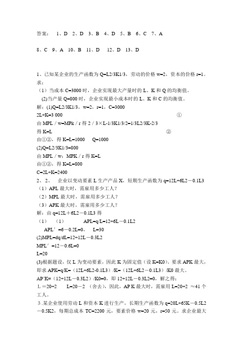
答案:1、D 2、D 3、B 4、D 5、B 6、C 7、A8、C 9、A 10、B 11、D 12、D 13、D1、已知某企业的生产函数为Q=L2/3K1/3,劳动的价格w=2,资本的价格r=1。
求:(1)当成本C=3000时,企业实现最大产量时的L、K和Q的均衡值。
(2)当产量Q=800时,企业实现最小成本时的L、K和C的均衡值。
解:(1)Q=L2/3K1/3,w=2,r=1,C=30002L+K=3 000 ①由MPL/w=MPk/r得2/3×L-1/3K1/3/2=1/3L2/3K-2/3得K=L ②由①②,得K=L=1000 Q=1000(2)Q=L2/3K1/3=800由MPL/w:MPK/r得K=L由①②,得K=L=800C=2L+K=24002、 2、企业以变动要素L生产产品X,短期生产函数为q=12L+6L2-0.1L3 (1)APL最大时,需雇用多少工人?(2)MPL最大时,需雇用多少工人?(3)APK最大时,需雇用多少工人?解:由q=12L+6L2-0.1L3得(1)(1)APL=q/L=12+6L-0.1L2APL'=6-0.2L=0,L=30(2)MPL=dq/dL=12+12L-0.3L2MPL'=12-0.6L=0L=20(3)根据题设,仅L为变动要素,因此K为固定值(设K=K0)。
要求APK最大,即求APK=q/K=(12L+6L2-0.1L3)/K=(12L+6L2-0.1L3)/K0最大。
AP΄K=(12+12L-0.3L2)/K0=0,即12+12L-0.3L2=0,解之得:L=20+2 L=20-2 (舍去),因此,AP K最大时,需雇用L=20+2 ≈41个工人。
3.某企业使用劳动L和资本K进行生产,长期生产函数为q=20L+65K-0.5L2-0.5K2,每期总成本TC=2200元,要素价格w=20元,r=50元。
求企业最大产量,以及L和K的投入量。
(完整版)微观经济学第4章生产论习题与答案
第4章生产论【练习及思考】参考答案要点1.填空题(1)总产量曲线、平均产量曲线和边际产量曲线都呈现出先上升,而后达到最大值以后,再呈现出下降的趋势。
其中,边际产量最先达到最大值,而后开始下降并与平均产量的最大值相交。
(2)边际产量的变化随着可变要素投入的增加一般经历两个阶段,即递增和递减两个阶段。
(3)按照生产过程中使用的生产要素的搭配情况可将那生产函数分为两种类型固定比例生产函数和可变比例生产函数。
2.判断题(下列判断正确的在括号内打√,不正确的打×)1)(√)在一种可变投入生产函数中,可变要素合理投入区域应在AP>MP>0的阶段。
2)(×)在一种可变投入生产函数中,可变要素合理投入区域应在MP>AP的第一阶段。
3)(√)生产理论中的短期是指未能调整全部生产要素的时期。
4)(×)AP曲线与MP曲线交于MP曲线的最高点。
5)(×)能提供相同效用的不同商品数量组合的点的连线即为等产量曲线。
6)(×)等产量曲线表示的是用同样数量劳动和资本生产不同的产量。
7)(√)当劳动的边际产量小于其平均产量时,平均产量肯定是下降的。
8)(×)边际产量递减,平均产量也递减。
9)(√)在生产的第Ⅱ阶段,AP是递减的。
3.选择题1)理性的生产者选择的生产区域应是(CD)。
A.MP>AP阶段B.MP下降阶段C.AP>MP>0阶段D.MP与AP相交之点起至MP与横轴交点止2)下列说法中正确的是(AC)。
A.只要总产量减少,边际产量一定为负B.只要MP减少,总产量一定减少C.MP曲线必定交于AP曲线的最高点D.只要MP减少,AP 也一定减少3)最优生产要素组合点上应该有(ABD)。
A.等产量曲线和等成本线相切B.MRTS LK=w/rC.dk/dl=w/rD.MP L/MP k=w/r4)等产量曲线上任意两点的产量肯定是(A )。
A.相等B.不等C.无关D.以上情况都存在5)若横轴代表劳动,纵轴表示资本,且劳动的价格为w,资本的价格为r,则等成本线的斜率为(C )。
西方经济学(微观经济学)课后练习答案第四章
习题一、名词解释生产函数边际产量边际报酬递减规律边际技术替代率递规律等产量线等成本线规模报酬扩展线二、选择题1、经济学中,短期是指()A、一年或一年以内的时期B、在这一时期内所有投入要素均是可以变动的C、在这一时期内所有投入要至少均是可以变动的。
D、在这时期内,生产者来不及调整全部生产要素的数量,至少有一种生产要素的数量是固定不变的。
2、对于一种可变要素投入的生产函数QfL,所表示的厂商要素投入的合理区域为(D)A、开始于AP的最大值,终止于TP的最大值B、开始于AP与MP相交处,终止于MP等于零C、是MP递减的一个阶段D、以上都对3、当MP L AP L时,我们是处于(A)A、对于L的Ⅰ阶段B、对K的Ⅲ阶段C、对于L的Ⅱ阶段D、以上都不是4、一条等成本线描述了()A、企业在不同产出价格下会生产的不同数量的产出B、投入要素价格变化时,同样的成本下两种投入要素的不同数量C、一定的支出水平下,企业能够买到的两种投入要素的不同组合D、企业能够用来生产一定数量产出的两种投入要素的不同组合5、当单个可变要素的投入量为最佳时,必然有:A.总产量达到最大B.边际产量达到最高C.平均产量大于或等于边际产量D.边际产量大于平均产量6、当平均产量递减时,边际产量是()A、递减B、为负C、为零D、以上三种可能都有7、以下有关生产要素最优组合,也即成本最小化原则的描述正确的一项是().A.MPL/r L=MPK/r KB.MRTS LK=r L/r KC.P MPr KKD.A和B均正确8、等产量曲线上各点代表的是()A.为生产同等产量而投入的要素价格是不变的B.为生产同等产量而投入的要素的各种组合比例是不能变化的C.投入要素的各种组合所能生产的产量都是相等的D.无论要素投入量是多少,产量是相等的9、如果厂商甲的劳动投入对资本的边际技术替代率为13,厂商乙的劳动投入对资本的边际技术替代率为23,那么(D)A.只有厂商甲的边际技术替代率是递减的B.只有厂商乙的边际技术替代率是递减的C.厂商甲的资本投入是厂商乙的两倍D.如果厂商甲用3单位的劳动与厂商乙交换2单位的资本,则厂商甲的产量将增加10、如果等成本曲线围绕它与纵轴的交点逆时针转动,那么将意味着(A)A.横轴表示的生产要素的价格下降B.纵轴表示的生产要素的价格上升C.横轴表示的生产要素的价格上升D.纵轴表示的生产要素的价格下降11、若等成本曲线在坐标平面上与等产量曲线相交,那么该交点表示的产量水平()A.应增加成本支出B.应减少成本支出C.不能增加成本支出D.不能减少成本支出12、在规模报酬不变的阶段,若劳动的使用量增加5%,而资本的使用量不变,则()A.产出增加5%B.产出减少5%C.产出的增加少于5%D.产出的增加大于5%13、规模报酬递减是在下述哪种情况下发生的()A、按比例连续增加各种生产要素B、不按比率连续增加各种生产要素C、连续地投入某种生产要素而保持其他生产要素不变D、上述都正确14、下列说法中正确的是(D)A、生产要素的边际替代率递减是规模报酬递减造成的B、边际收益递减是规模报酬递减规律造成的C、规模报酬递减是边际收益递减规律造成的D、生产要素的边际技术替代率递减是边际收益递减规律造成的15、当某厂商以最小成本生产出既定产量时(D)A、总收益为零B、获得最大利润C、没有获得最大利润D、无法确定是否获得了最大总利润三、判断题1、随着某种生产要素投入量的增加,边际产量和平均产量到一定程度将趋于下降,其中边际产量的下降一定先于平均产量。
微观经济学第四章习题答案完整版

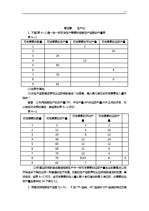
微观经济学第四章习题答案HEN system office room 【HEN16H-HENS2AHENS8Q8-HENH1688】第四章生产论1. 下面(表4—1)是一张一种可变生产要素的短期生产函数的产量表:可变要素的数量可变要素的总产量可变要素的平均产量可变要素的边际产量122103244125606677080963(2)该生产函数是否表现出边际报酬递减如果是,是从第几单位的可变要素投入量开始的解答:(1)利用短期生产的总产量(TP)、平均产量(AP)和边际产量(MP)之间的关系,可以完成对该表的填空,其结果如表4—2所示:可变要素的数量可变要素的总产量可变要素的平均产量可变要素的边际产量1222212610324812448122456012126661167701048708\f(34)09637-7高点以后开始逐步下降的这样一种普遍的生产现象。
本题的生产函数表现出边际报酬递减的现象,具体地说,由表4—2可见,当可变要素的投入量从第4单位增加到第5单位时,该要素的边际产量由原来的24下降为12。
2. 用图说明短期生产函数Q=f(L,eq \o(K,\s\up6(-)))的TPL曲线、APL 曲线和MPL曲线的特征及其相互之间的关系。
解答:短期生产函数的TPL曲线、APL曲线和MPL曲线的综合图如图4—1所示。
图4—1由图4—1可见,在短期生产的边际报酬递减规律的作用下,MPL曲线呈现出先上升达到最高点A以后又下降的趋势。
从边际报酬递减规律决定的MPL曲线出发,可以方便地推导出TPL 曲线和APL曲线,并掌握它们各自的特征及相互之间的关系。
关于TPL 曲线。
由于MPL=eq \f(d TP L,d L),所以,当MP L>0时,TP L曲线是上升的;当MPL <0时,TPL曲线是下降的;而当MPL=0时,TPL曲线达最高点。
换言之,在L=L3时,MPL曲线达到零值的B点与TPL曲线达到最大值的B′点是相互对应的。
人大版微观经济学(第三版)课后答案第3-4章

第三章 消费者选择第一部分 教材配套习题本习题详解1.已知一件衬衫的价格为80元,一份肯德基快餐的价格为20元,在某消费者关于这两种商品的效用最大化的均衡点上,一份肯德基快餐去替代衬衫的边际替代率MRS是多少?解答:用 X 表示肯德基快餐的份数;Y 表示衬衫的件数;MRSXY 表示在 维持效用水平不变的前提下,消费者增加一份肯德基快餐消费时所需要放弃的衬衫的消费数量。
在该消费者实现关于这两种商品的效用最大化时,在均衡点上有边际替代率等于价格比,则有:201804X XY Y P Y MRS X P ∆=-===∆ 它表明,在效用最大化的均衡点上,该消费者关于一份肯德基快餐对衬衫 的边际替代率MRS为0.25。
2.假设某消费者的均衡如图3—21所示。
其中,横轴OX1和纵轴OX2分别表示商品1和商品2的数量,线段AB为消费者的预算线,曲线U 为消费者的无差异曲线,E点为效用最大化的均衡点。
已知商品1的价格P1=2元。
求: (1)求消费者的收入; (2)求商品2的价格P2; (3)写出预算线方程; (4)求预算线的斜率; (5)求E点的MRS12的值。
图3—21 某消费者的均衡解答:(1)横轴截距表示消费者的收入全部购买商品1的数量为30单位,且已知P1=2元,所以,消费者的收入 M=2×30=60元。
(2)图3—1中纵轴截距表示消费者的收入全部购买商品2的数量为20单位,且由(1)已知收入 M=60元,所以,商品2的价格P 2=M 20=6020=3(元)。
(3)由于预算线方程的一般形式为 P 1X 1+P 2X 2=M,所以本题预算线方程具体写为:2X 1+3X 2=60。
(4)(4)将(3)中的预算线方程进一步整理为X 2=-23X 1+20。
所以,预算线的斜率为-23。
(5)在消费者效用最大化的均衡点E 上,有211212X PMRS X P ∆=-=∆,即无差异曲线斜率的绝对值即MRS 等于预算线斜率的绝对值P 1P 2。
西方经济学(微观经济学)课后练习答案第四章
习 题一、名词解释生产函数 边际产量 边际报酬递减规律 边际技术替代率递规律 等产量线 等成本线 规模报酬 扩展线二、选择题1、经济学中,短期是指( )A 、一年或一年以内的时期B 、在这一时期内所有投入要素均是可以变动的C 、在这一时期内所有投入要至少均是可以变动的。
D 、在这时期内,生产者来不及调整全部生产要素的数量,至少有一种生产要素的数量是固定不变的。
2、对于一种可变要素投入的生产函数()Q f L =,所表示的厂商要素投入的合理区域为( D )A 、开始于AP 的最大值,终止于TP 的最大值B 、开始于AP 与MP 相交处,终止于MP 等于零C 、是MP 递减的一个阶段D 、以上都对3、当L L MP AP >时,我们是处于( A )A 、对于L 的Ⅰ阶段B 、对K 的Ⅲ阶段C 、对于L 的Ⅱ阶段D 、以上都不是4、一条等成本线描述了( )A 、企业在不同产出价格下会生产的不同数量的产出B 、投入要素价格变化时,同样的成本下两种投入要素的不同数量C 、一定的支出水平下,企业能够买到的两种投入要素的不同组合D 、企业能够用来生产一定数量产出的两种投入要素的不同组合5、当单个可变要素的投入量为最佳时,必然有:A. 总产量达到最大B. 边际产量达到最高C. 平均产量大于或等于边际产量D. 边际产量大于平均产量6、当平均产量递减时,边际产量是( )A 、递减B 、为负C 、为零D 、以上三种可能都有7、以下有关生产要素最优组合,也即成本最小化原则的描述正确的一项是(). A.MPL /r L =MPK /r KB.MRTS LK =r L /r KC.K P MP ⋅=r KD.A和B均正确8、等产量曲线上各点代表的是( )A.为生产同等产量而投入的要素价格是不变的B.为生产同等产量而投入的要素的各种组合比例是不能变化的C.投入要素的各种组合所能生产的产量都是相等的D.无论要素投入量是多少,产量是相等的9、如果厂商甲的劳动投入对资本的边际技术替代率为13,厂商乙的劳动投入对资本的边际技术替代率为23,那么(D )A.只有厂商甲的边际技术替代率是递减的B.只有厂商乙的边际技术替代率是递减的C.厂商甲的资本投入是厂商乙的两倍D.如果厂商甲用3单位的劳动与厂商乙交换2单位的资本,则厂商甲的产量将增加10、如果等成本曲线围绕它与纵轴的交点逆时针转动,那么将意味着(A )A.横轴表示的生产要素的价格下降B.纵轴表示的生产要素的价格上升C.横轴表示的生产要素的价格上升D.纵轴表示的生产要素的价格下降11、若等成本曲线在坐标平面上与等产量曲线相交,那么该交点表示的产量水平()A.应增加成本支出B.应减少成本支出C.不能增加成本支出D.不能减少成本支出12、在规模报酬不变的阶段,若劳动的使用量增加5%,而资本的使用量不变,则()A.产出增加5%B.产出减少5%C.产出的增加少于5%D.产出的增加大于5%13、规模报酬递减是在下述哪种情况下发生的()A、按比例连续增加各种生产要素B、不按比率连续增加各种生产要素C、连续地投入某种生产要素而保持其他生产要素不变D、上述都正确14、下列说法中正确的是(D )A、生产要素的边际替代率递减是规模报酬递减造成的B、边际收益递减是规模报酬递减规律造成的C、规模报酬递减是边际收益递减规律造成的D、生产要素的边际技术替代率递减是边际收益递减规律造成的15、当某厂商以最小成本生产出既定产量时(D )A、总收益为零B、获得最大利润C、没有获得最大利润D、无法确定是否获得了最大总利润三、判断题1、随着某种生产要素投入量的增加,边际产量和平均产量到一定程度将趋于下降,其中边际产量的下降一定先于平均产量。
曼昆微观经济学第四章课后答案
排列。
因为在其他因素不变时,价格上
升,供给量上升,所以供给曲线向右上方倾斜。
8
.生产者技术的变动引起了沿着供给曲线的变动,还是供给曲线的移动?价格的变化引起了沿着供给曲线
17
5
.考虑DVD
、电视和电影院门票市场。
A
.对每一对物品,确定它们是互补品还是替代品
·DVD
和电视
·DVD
和电影票
·电视和电影票
答:DVD 和电视机是互补品,因为不可能在没有电视的情况下看DVD。DVD 和电影票是替代品,因为一
部电影即可以在电影院看,也可以在家看。电视和电影
的变动,还是供给曲线的移动?
答:生产者技术的变动引起了供给曲线的移动,价格变化引起了沿着供给曲线的变动。
9
.给市场均衡下定义,描述使市场向均衡变动的力量。
答:当供给与需求达到了平衡的状态,即需求曲线与供给曲线相交于一点时,这一点叫做市场的均衡。使市
场达到均衡的力量是价格。当价格低于均衡价格时,市场上求大于供,供给者发现提高价格也不会减少销售量,
20
图4—16 自由体操着装的规定对运动衫市场的影响
D
.发明了新织布机。
答:新织布机的发明使运动衫
生产的技术水平提高,使运动衫的供给曲线向右下方移动,运动衫的价格下降,
均衡数量增加。
图4—17 新织布机的发明对运动衫市场影响
8
.调查表明,年轻人吸食的毒品增加了。在随后的争论中,
C
.工程师开发出用于家用旅行车生产的新的自动化机器。
答:决定供给的技术因素受影响,生产技术提高,会使家用旅行车的供给增加。
微观经济学答案解析第四章生产论
第四章生产论1. 下面(表4—1)是一张一种可变生产要素的短期生产函数的产量表:(2)该生产函数是否表现出边际报酬递减?如果是,是从第几单位的可变要素投入量开始的?解答:(1)利用短期生产的总产量(TP)、平均产量(AP)和边际产量(MP)之间的关系,可以完成对该表的填空,其结果如表4—2所示:开始逐步下降的这样一种普遍的生产现象。
本题的生产函数表现出边际报酬递减的现象,具体地说,由表4—2可见,当可变要素的投入量从第4单位增加到第5单位时,该要素的边际产量由原来的24下降为12。
2. 用图说明短期生产函数Q=f(L,K-)的TP L曲线、AP L曲线和MP L曲线的特征及其相互之间的关系。
解答:短期生产函数的TP L 曲线、AP L 曲线和MP L 曲线的综合图如图4—1所示。
图4—1由图4—1可见,在短期生产的边际报酬递减规律的作用下,MP L 曲线呈现出先上升达到最高点A 以后又下降的趋势。
从边际报酬递减规律决定的MP L 曲线出发,可以方便地推导出TP L 曲线和AP L 曲线,并掌握它们各自的特征及相互之间的关系。
关于TP L 曲线。
由于MP L =d TP L d L,所以,当MP L >0时,TP L 曲线是上升的;当MP L<0时,TP L 曲线是下降的;而当MP L =0时,TP L 曲线达最高点。
换言之,在L =L 3时,MP L 曲线达到零值的B 点与TP L 曲线达到最大值的B ′点是相互对应的。
此外,在L <L 3即MP L >0的范围内,当MP ′L >0时,TP L 曲线的斜率递增,即TP L 曲线以递增的速率上升;当MP ′L <0时,TP L 曲线的斜率递减,即TP L 曲线以递减的速率上升;而当MP ′=0时,TP L 曲线存在一个拐点,换言之,在L =L 1时,MP L 曲线斜率为零的A 点与TP L 曲线的拐点A ′是相互对应的。
关于AP L 曲线。
由于AP L =TP LL ,所以,在L =L 2时,TP L 曲线有一条由原点出发的切线,其切点为C 。
微观经济学第四章完全竞争市场(含答案)
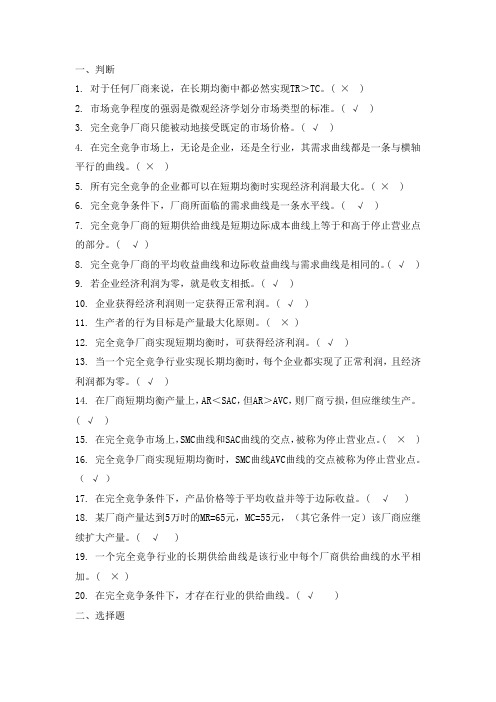
一、判断1. 对于任何厂商来说,在长期均衡中都必然实现TR>TC。
( × )2. 市场竞争程度的强弱是微观经济学划分市场类型的标准。
( √ )3. 完全竞争厂商只能被动地接受既定的市场价格。
( √ )4. 在完全竞争市场上,无论是企业,还是全行业,其需求曲线都是一条与横轴平行的曲线。
( × )5. 所有完全竞争的企业都可以在短期均衡时实现经济利润最大化。
( × )6. 完全竞争条件下,厂商所面临的需求曲线是一条水平线。
( √ )7. 完全竞争厂商的短期供给曲线是短期边际成本曲线上等于和高于停止营业点的部分。
( √ )8. 完全竞争厂商的平均收益曲线和边际收益曲线与需求曲线是相同的。
( √ )9. 若企业经济利润为零,就是收支相抵。
( √ )10. 企业获得经济利润则一定获得正常利润。
( √ )11. 生产者的行为目标是产量最大化原则。
( × )12. 完全竞争厂商实现短期均衡时,可获得经济利润。
( √ )13. 当一个完全竞争行业实现长期均衡时,每个企业都实现了正常利润,且经济利润都为零。
( √ )14. 在厂商短期均衡产量上,AR<SAC,但AR>AVC,则厂商亏损,但应继续生产。
( √ )15. 在完全竞争市场上,SMC曲线和SAC曲线的交点,被称为停止营业点。
( × )16. 完全竞争厂商实现短期均衡时,SMC曲线AVC曲线的交点被称为停止营业点。
(√)17. 在完全竞争条件下,产品价格等于平均收益并等于边际收益。
( √ )18. 某厂商产量达到5万时的MR=65元,MC=55元,(其它条件一定)该厂商应继续扩大产量。
( √ )19. 一个完全竞争行业的长期供给曲线是该行业中每个厂商供给曲线的水平相加。
( × )20. 在完全竞争条件下,才存在行业的供给曲线。
( √ )二、选择题1.下列哪一种说法不是完全竞争市场的特征( B )。
微观经济学课件及课后答案4
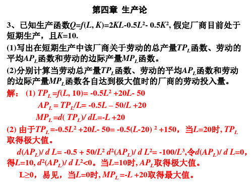
3、已知生产函数Q=f(L, K)=2KL-0.5L2- 0.5K2, 假定厂商目前处于 短期生产,且K=10.
(1)写出在短期生产中该厂商关于劳动的总产量TPL函数、劳动的 平均APL函数和劳动的边际产量MPL函数。 (2)分别计算当劳动总产量TPL函数、劳动的平均APL函数和劳动 的边际产量MPL函数各自达到极大值时的厂商的劳动投入量。 解: (1) TPL =f(L, 10)= -0.5L2 +20L- 50
产的扩展线方程为K 3
L 3
,
即 2L
10 L1/ 3 K 1/ 3 3
PK K / PL
PK
5 L2/ 3 K 2/ 3 3
P, L
当PL=1,PK=1, Q=1000时,厂商长期生产的扩展线方程为2L=K.
厂商实现最小成本的要素投入组合满足下列方程组
所以 ,
2L K
Q
5L1/ 3 K 2/ 3
6、假设某厂商的短期生产函数为 Q 35L 8L2 L3 。 求:(1)该企业的平均产量函数和边际产量函数。 (2)如果企业使用的生产要素的数量 L=6,是否处于短期生产的合理区间? 为什么? 解:(1)平均产量函数 APL Q / L 35 8L L2 ,
边际产量函数 M PL d Q/ dL3 5 1 6 L 23 L (2)当 APL MPL 时,L=4(取正根);当 MPL=0 时,L=7(取正根)。 当企业使用的生产要素的数量 L=6,介于 4 与 7 之间,处于短期生产的合 理区间。
1000
L 100 3 2, K 200 3 2
(2)
Q KL,
KL
Q K
(K
L2 L)2
,
Q L
微观经济学课后练习题参考答案4
第四章 生产论一、选择题:二、名词解释:1、边际产量:指最后一单位生产要素的投入,所带来的总产量的变化量,简称MP2、平均产量:指平均每单位生产要素投入的产出量,简称AP3、边际报酬递减规律:在技术水平不变的情况下,当把一种可变的生产要素投入到一种或几种不变的生产要素中时,最初这种生产要素的增加会使产量增加,但当它的增加超过一定程度时,增加的产量将要递减。
4、等产量线:表示其它条件不变时,为生产一定的产量所需投入的两种生产要素之间的各种可能组合的轨迹。
5、边际技术替代率:指在产量不变的情况下,当某种生产要素增加一单位时,与另一生产要素所减少的数量的比率。
6、等成本线:指在生产要素价格不变的情况下,生产者花费一定的总成本能购买的两种生产要素最大可能性组合的轨迹。
7、扩展线:指在技术既定和要素价格不变情况下,不同产量水平的最优投入组合点的轨迹。
即不同产量的等产量曲线与等成本线相切的切点联接起来所形成的曲线。
8、规模报酬:规模报酬就是探讨这样一种投入—产出的数量关系,当各种要素同时增加或减少一定比率时,生产规模变动所引起产量的变化情况。
9、规模经济:是指随着生产规模扩大,产品平均成本下降的情况。
三、问答题:1、分析说明生产要素投入的经济区域。
答:生产要素投入的经济区域又称生产要素的合理投入区,指理性的生产者所限定的生产要素投入的数量范围。
具体讲,要分短期和长期两种情况来分析。
(1)如果生产处于短期,并且只有一种生产要素投入数量是可变的,那么该要素的合理投入区处于平均产量最大值点与边际产量等于0的点之间,即L 3<L ﹤L 4 ,在L 3的左边,生产要素投入L 的边际产量超过此时的平均水平,相对于固定投入而言,变动投入数量相对不足,所以理性的生产者不会把投入数量停留在这一范围内。
而在L 4的右边,L 的边际产量为负,很显然,厂商不会把投入增加到这一范围内。
由此可见,如何理性的生产者既不会将生产停留在第Ⅰ阶段,也不会将生产扩张到第Ⅲ阶段,所以,生产只能在第Ⅱ阶段进行。
微观经济学第四章课后练习答案

1、什么是欲望和效用?马斯洛把人的欲望分为哪五个层次?效用和使用价值的关系.答:1)欲望是一种缺乏的感觉与求得满足的愿望。
这也就是说,欲望是不足之感与求足之愿的统一,两者缺一都不能称为欲望。
2)效用是从消费某种物品中所得到的满足程度。
3)马斯洛把人的欲望分为五个层次:第一,基本生理的需要,这是人类最基本的欲望;第二,安全的需要;第三,归属和爱的需要;第四,尊重的需要,这是人更高层次的社会需要;第五,自我实现的需要,这是人最高层次的欲望.2、基数效用论和序数效用论的基本观点是什么?它们各采用何种分析方法?答:1)基数效用论基本观点是:效用是可以用计量并加总求和的,效用的大小是可以用基数(1,2,3…)来表示,正如长度单位可以用米来表示一样。
2)序数效用论是为了弥补基数效用论的缺点而提出来的另一种研究消费者行为的理论。
其基本观点是:效用作为一种心理现象无法计量,也不能加总求和,只能表示出满足程度的高低与顺序,因此,效用只能用序数(第一、第二、第三…)来表示.3)基数效用论采用的是边际效用分析法;序数效用论采用的是无差异曲线分析法.3、什么叫“边际”?总效用和边际效用的关系如何?答:1)边际的含义是增量,指自变量增加1单位所引起的因变量的增加量.2)总效用是指从消费一定量某种物品中所得到的总满足程度;边际效用是指某种物品的消费量每增加1单位所增加的满足程度.消费量变动做引起的效用的变动即位边际效用。
当边际效用为正数时,总效用是增加的;但边际效用为零时,总效用达到最大;当边际效用为负数时,总效用减少。
4、什么是边际效用递减规律?边际效用为什么递减?答:1)随着消费者对某种物品消费量的增加,他从该物品连续增加的消费单位中所得到的边际效用是递减的,这就被称为边际效用递减规律.2)认为边际效用递减规律成立的学派,用两个理由来支持他们的论断。
一是从人的生理和心理的角度来进行解释,认为随着相同消费品的连续增加,从每一单位消费品中所感受到的满足程度和对重复刺激的反应程度是递减的.二是从商品的多用途的角度来进行解释,认为消费者总是将第一单位的消费品用在最重要的用途上,第二单位的消费品用在次重要的用途上,如此等等.这样,消费品的边际效用,就随消费品的用途重要性的递减而递减。
微观经济学 --- 第四章{生产者理论} 参考答案 (上海商学院)
第四章 参考答案一、名词解释1.生产者(producer)是指能够对生产和销售做出统一生产决策,且努力将若干种投入转化为产出的经济单位。
2.生产函数(product function)是指在一定时期内,在技术水平不变的情况下,生产中所运用的各种生产要素的数量和能产生的最大产量之间的关系。
3.生产要素(factors of production)一般是指劳动、土地、资本和企业家才能等。
4.固定比例投入生产函数(fixed-ratio input product function)的形式可以描述为⎪⎭⎫⎝⎛=v K u L Q ,min ,其中Q 为产量,L 、K 分别为劳动和资本的投入量,u 、v 分别为劳动和资本的生产技术系数,表示生产一单位产品所需的劳动和资本投入量。
5.一种可变要素的生产函数:表示在技术水平和其他投入不变的条件下,一种可变生产要素的投入量与其所生产的最大产量之间的关系的函数。
6.短期生产(short-run production)是指生产者来不及调整全部生产要素的数量,至少有一种生产要素的数量是固定不变的时间周期。
7.长期生产(long-run production)是指生产者可以调整全部生产要素的时间周期。
8.柯布----道格拉斯生产函数(Cobb-Douglas product function)的形式可以描述为βαK AL Q =,其中Q 为产量,L 、K 分别为劳动和资本投入量,A 、α和β为参数,α和β分别表示劳动和资本所得在总产量中所占份额,α<0,β<0。
9.总产量(total product)是指与一定的可变要素劳动的投入量相对应的最大产量。
10.平均产量(average product)是总产量与所使用的可变要素劳动的投入之比。
11.边际产量(marginal product)是增加一单位可变要素劳动投入量所增加的产量。
12.边际报酬递减规律(law of diminishing marginal returns)是指在技术水平不变的条件下,连续等量地把一种可变生产要素增加到其他生产要素数量不变的生产过程中,当这种生产要素的投入量小于某一特定值时,增加该要素投入所带来的边际产量是递增的,超过这个特定值时,所带来的边际产量是递减的。
平狄克《微观经济学》课后答案 3-4

CHAPTER 3CONSUMER BEHAVIORChapter 3 builds the foundation to derive the demand curve in Chapter 4. In order to understand demand theory, students must have a firm grasp of indifference curves, the marginal rate of substitution, the budget line, and optimal consumer choice. Utility theory may be discussed independently from consumer choice. Many students find utility functions to be a more abstract concept than preference relationships. However, if you plan to discuss uncertainty in Chapter 5, you will need to cover marginal utility. Even if you cover utility theory only briefly, make sure students are comfortable with the term utility because it appears frequently in Chapter 4.When introducing indifference curves, stress that physical quantities are represented on the two axes. After discussing supply and demand, students may think that price should be on the vertical axis. To develop indifference curves, start with any point in the Cartesian plane and ask for points that are more (and less) preferred. This will divide the plane into four quadrants. Then ask between which points they will be indifferent. Once students grasp the concept of preference points, introduce the notion of a “preference hill.” Using the example of a topographical map or a well-drawn three dimensional figure, point out that a three-dimensional figure is being collapsed into two dimensions.The marginal rate of substitution, MRS , is confusing to students. Some confuse the MRS with the ratio of the two quantities. If this is the case, point out that the slope is equal to the ratio of the rise, ∆Y, and the run, ∆X . This ratio is equal to the ratio of the intercepts of a line just tangent to the indifference curve. As we move along a convex indifference curve, these intercepts and the MRS change. Another problem is the terminology “of X for Y .” This is confusing because we are not substituting “X for Y ,” but Y for one unit of X . Exercise (6) discusses this point, but you may want to offer other exercises to stress it.1. What does transitivity of preferences mean?Transitivity of preferences implies that if someone prefers A to B and prefers B to C , then he orshe prefers A to C .satisfaction. This trading continues until the highest level of satisfaction is achieved.6. Explain why consumers are likely to be worse off when a product that they consume is rationed.If the maximum quantity of a good is fixed by decree and desired quantities are not available forpurchase, then there is no guarantee that the highest level of satisfaction can be achieved. Theconsumer will not be able to give up the consumption of other goods in order to obtain more of therationed good. Only if the amount rationed is greater than the desired level of consumption canthe consumer still maximize satisfaction without constraint. (Note: rationing may imply ahigher level of social welfare because of equity or fairness considerations across consumers.)7. Upon merging with West Germany’s economy, East German consumers indicated a preference for Mercedes-Benz automobiles over Volkswagen automobiles. However, when they converted their savings into deutsche marks, they flocked to Volkswagen dealerships. How can you explain this apparent paradox?Three assumptions are required to address this question: 1) that a Mercedes costs more than aVolkswagen; 2) that the East German consumers’ utility function comprises two goods,automobiles and all other goods evaluated in deutsche marks; and 3) that East Germans haveincomes. Based on these assumptions, we can surmise that while once-East German consumersmay prefer a Mercedes to a Volkswagen, they either cannot afford a Mercedes or they prefer abundle of other goods plus a Volkswagen to a Mercedes alone.8. Describe the equal marginal principle. Explain why this principle may not hold if increasing marginal utility is associated with the consumption of one or both goods.The equal marginal principle states that the ratio of the marginal utility to price must be equalacross all goods to obtain maximum satisfaction. This explanation follows from the same logicexamined in Review Question 5. Utility maximization is achieved when the budget is allocatedso that the marginal utility per dollar of expenditure is the same for each good.If marginal utility is increasing, the consumer maximizes satisfaction by consuming ever largeramounts of the good. Thus, the consumer would spend all income on one good, assuming aconstant price, resulting in a corner solution. With a corner solution, the equal marginalprinciple cannot hold.9. What is the difference between ordinal utility and cardinal utility? Explain why the assumption of cardinal utility is not needed in order to rank consumer choices.Ordinal utility implies an ordering among alternatives without regard for intensity of preference.For example, the consumer’s first choice is preferred to their second choice. Cardinal utilityimplies that the intensity of preferences may be quantified. An ordinal ranking is all that isneeded to rank consumer choices. It is not necessary to know how intensely a consumer prefersbasket A over basket B; it is enough to know that A is preferred to B.10. The price of computers has fallen substantially over the past two decades. Use this drop in price to explain why the Consumer Price Index is likely to substantially understate the cost-of-living index for individuals who use computers intensively.The consumer price index measures the changes in the weighted average of the prices of thebundle of goods purchased by consumers. The weights equal the share of consumer's expenditureson all of the goods in the bundle. A base year is chosen, and the weights for that year are used tocompute the CPI in that and subsequent years. When the price of a good falls substantially then aconsumer will substitute towards that good, altering the share of that consumer's income spent oneach good. By using the base year's weights the CPI does not take into account that large pricechanges alter these expenditure shares, and so gives an inaccurate measure of changes in the costof living.For example, assume Fred spends 10% of his income on computers in 1970, and that Fred'sexpenditure shares in 1970 were used as the weights to calculate Fred's CPI in subsequent years.If Fred's demand for computers was inelastic, then reductions in the price of computers (relativeto other goods) would reduce the share of his income spent on computers. After 1970 a CPI thatused Fred's 1970 expenditure shares as weights would give a 10% weight to the falling price ofcomputers, even though Fred spent less that 10% of his income on computers. So long as theprices of other goods rose, or fell less than 10%, then the CPI gives too little weight to the changesin the prices of other goods, and understates the changes in Fred's cost of living.1. In this chapter, consumer preferences for various commodities did not change during the analysis. Yet in some situations, preferences do change as consumption occurs. Discuss why and how preferences might change over time with consumption of these two commodities:a. cigarettesThe assumption that preferences do not change is a reasonable one if choices are independentacross time. It does not hold, however, when “habit-forming” or addictive behavior is involved, asin the case of cigarettes: the consumption of cigarettes in one period influences their consumptionin the next period.b. dinner for the first time at a restaurant with a special cuisineWhile there may not be anything physically addictive in dining at new and different restaurants, one can become better informed about a particular restaurant. One may enjoy choosing more new and different restaurants, or one may be tired of choosing another new and different place to4.a.c. tothis graphically?, the quantity of butter by B, the Let Bill’s income be represented by Y, the price of butter by PB, and the quantity of margarine by M. Then the general form of the price of margarine by PMbudget constraint is:5.the their a.c. If both Smith and Jones pay the same prices for their refreshments, will their marginal rates ofsubstitution of alcoholic for nonalcoholic drinks be the same or different? Explain.In order to maximize utility, the consumer must consume quantities such that the MRS betweenany two commodities is equal to the ratio of prices. If Smith and Jones are rational consumers,their MRS must be equal because they face the same market prices. But because they havedifferent preferences, they will consume different amounts of the two goods, alcoholic andnonalcoholic. At those different levels, however, their MRS are equal.6. Anne is a frequent flyer whose fares are reduced (through coupon giveaways) by 25 percent after she flies 25,000 miles a year, and then by 50 percent after she flies 50,000 miles. Can you graph the budget line that Anne faces in making her flight plans for the year?In Figure 3.6, we plot miles flown, M , against all other goods, G , in dollars. The budgetconstraint is:Y = P M M + P G G , or.⎪⎪⎭⎫ ⎝⎛-=G M G P P M P Y G The slope of the budget line is -P P M G. In this case, the price of miles flown changes as the number of miles flown changes, so the budget curve is kinked at 25,000 and at 50,000 miles. Suppose P M is $1 per mile for less than or equal to 25,000 miles. Then P M = $0.75 for 25,000 < M ≥ 50,000 and P M = $0.50 for M > 50,000. Also, let P G = $1.00. Then the slope of the budget line from A to B is -1, the slope of the budget line from B to C is -0.75, and the slope of the budget line from B to D is -0.5.8. Suppose that Samantha and Jason both spend $24 per week on video and movie entertainment.U = 12 U = 24Food Clothing Food Clothing 1.0 12.0 1.0 24.01.5 8.02.0 12.02.0 6.03.0 8.012 = 1F + 3C , or ⎪⎪⎭⎝-=34.See Figure 3.10.a.c. What is the utility-maximizing choice of food and clothing? (Hint: Solve the problemgraphically.)The highest level of satisfaction occurs where the budget line is tangent to the highestindifference curve. In Figure 3.10.a this is at the point F = 6 and C = 2. To check this answer,note that it exhausts Jane’s income, 12 = 6P F + 2P C . Also, this bundle yields a satisfaction of 12,as (6)(2) = 12. See Figure 3.10.a.d. What is the marginal rate of substitution of food for clothing when utility is maximized?At the utility-maximizing level of consumption, the slope of the indifference curve is equal to theslope of the budget constraint. Since the MRS is equal to the negative slope of the indifferencecurve, the MRS in this problem is equal to one-third. Thus, Jane would be willing to give upone-third of a unit of clothing for one unit of food.e. Suppose that Jane buys 3 units of food and 3 units of clothing with her $12 budget. Would hermarginal rate of substitution of food for clothing be greater or less than 1/3? Explain.If Jane buys 3 units of food for $1.00 per unit and 3 units of clothing for $3.00 per unit, she wouldspend all her income. However, she would obtain a level of satisfaction of only 9, whichrepresents a sub-optimal choice. At this point, the MRS is greater than one-third, and thus, atthe prices she faces, she would welcome the opportunity to give up clothing to get more food. Sheis willing to trade clothing for food until her MRS is equal to the ratio of prices. See Figure3.10.c.Figure 3.10.c11. The utility that Meredith receives by consuming food F and clothing C is given by u(F,C) = FC. Suppose that Meredith’s income in 1990 is $1,200 and the prices of food and clothing are $1 per unit for each. However, by 1995 the price of food has increased to $2 and the price of clothing to $3. Let 100 represent the cost of living index for 1990. Calculate the ideal and the Laspeyres cost-of-living index for Meredith for 1995. (Hint: Meredith will spend equal amounts on food and clothing with these preferences.)Laspeyres IndexThe Laspeyres index represents how much more Meredith would have to spend in 1995 versus 1990 ifshe consumed the same amounts of food and clothing in 1995 as she did in 1990. That is, the Laspeyresindex for 1995 (L) is given by:L = 100 (Y ')/Ywhere Y’ represents the amount Meredith would spend at 1995 prices consuming the same amount offood and clothing as in 1990: Y ' = P 'F F + P 'C C = 2F + 3C, where F and C represent the amounts of foodand clothing consumed in 1990.We thus need to calculate F and C, which make up the bundle of food and clothing which maximizesMeredith’s utility given 1990 prices and her income in 1990. Use the hint to simplify the problem:Since she spends equal amounts on both goods, P F F = P C C. Or, you can derive this same equationmathematically: With this utility function, MU C = ∆U/∆C = F, and MU F = ∆U/∆F = C. To maximizeutility, Meredith chooses a consumption bundle such that MU F /MU C = P F /P C , which again yields P F F =P C C.From the budget constraint, we also know that:P F F +P C C = YCombining these two equations and substituting the values for the 1990 prices and income yields thesystem of equations:C = F and C + F = 1,200Solving these two equations, we find that:C = 600 and F = 600Therefore, the Laspeyres cost-of-living index is:L = 100(2F + 3C)/Y = 100[(2)(600) + (3)(600)]/1200 = 250Ideal IndexThe ideal index represents how much more Meredith would have to spend in 1995 versus 1990 if sheconsumed amounts of food and clothing in 1995 which would give her the same amount of utility as shehad in 1990. That is, the ideal index for 1995 (I) is given by:I = 100(Y'')/Y, where Y'' = P'F F + P'C C' = 2F' + 3C'where F' and C' are the amount of food and clothing which give Meredith the same utility as she had in1990. F' and C' must also be such that Meredith spends the least amount of money at 1995 prices toattain the 1990 utility level.The bundle (F',C') will be on the same indifference curve as (F,C) and the indifference curve at this point will be tangent to a budget line with slope -(P'F /P'C ), where P'F and P'C are the prices of food and clothing in 1995. Since Meredith spends equal amounts on the two goods, we know that 2F' = 3C'. Since this bundle lies on the same indifference curve as the bundle F = 600, C = 600, we also know that F'C' = (600)(600).Cslope 1P slope F C =-H K slope slope F C =-'H KFigure 3.11Solving for F' yields:F'[(2/3)F'] = 360,000 or F' =[(/),)]32360000 = 734.8From this, we obtain C':C' = (2/3)F' = (2/3)734.8 = 489.9We can now calculate the ideal index: I = 100(2F' + 3C')/Y = 100[2(734.8) + (3)(489.9)]/1200 = 244.9CHAPTER 4INDIVIDUAL AND MARKET DEMANDChapter 4 relies on two important ideas from Chapter 3: the influence of price and income changes on the budget line and optimal consumer choice. The chapter focuses on price changes, individual demand, market demand, demand elasticity, and consumer surplus. These concepts are crucial to understanding the application of demand and supply analysis in Chapter 9 as well as the discussion of market failure in Parts III and IV. Chapter 4 also discusses the derivation of the individual’s demand curve with a discussion of substitution and income effects. The analytical tools students learn in this chapter will be important for the discussion of factor supply and demand in Chapter 14.When discussing the derivation of demand, review how the budget curve pivots around an intercept as price changes and how optimal quantities change as the budget line pivots. Once students understand the effect of price changes on consumer choice, they can grasp the derivation of the price consumption path and the individual demand curve. Remind students that the price a consumer is willing to pay is a measure of the marginal benefit of consuming another unit.When covering the aggregation of individual demands, stress that this is equivalent to the summation of individual demand curves horizontally. Students might think that they can add linear demand functions, e.g., add Q P =-1 plus Q P =-23 to arrive at Q P =-35 or 223Q P =-. Students must be reminded, instead, to write the demand curve in inverse form, with price as a function of quantity, and then add. Thus, we add P = 1 - Q to P = 1 - 2Q to obtain P = 2 - 3Q .Price elasticity of demand and consumer surplus are referred to throughout the text, but the mathematics of price elasticity of demand is difficult for many students. Before discussing the algebra, encourage students to develop an intuitive grasp of elasticity as a measure of the sensitivity of the quantity demanded to changes in price.The easiest algebraic representation of elasticity is %%∆∆QP. As you expand on this expression, make sure thatstudents can distinguish between the slope of a line and an elasticity at each point. One effective teaching method is using a linear demand curve to show that while the slope is constant, the elasticity changes throughout the range of prices. The text relies on this relationship in the discussion of the monopolist’s determination of the profit-maximizing quantity in Chapter 10. The exercises given here are progressive in their difficulty, i.e., the last exercise is much harder than the first. Exercises (1) and (7) assume student understanding of demand elasticity, and a grasp of income elasticity is needed for Exercise (9).Although this chapter introduces consumer surplus, it is not extensively discussed until Chapter 9; producer surplus is covered in Chapter 8. If you postpone the discussion of consumer surplus, do not assign Exercise (4). Once students understand consumer surplus, they will find it to be an extremely useful tool. See Example 4.5.Section 4.2 discusses income and substitution effects. An understanding of these effects is aided by the discussion of normal and inferior goods. This is also a good time to reinforce the concept of relative prices, i.e., a decrease in the price of one good increases the relative price of the other good. Giffen goods, while infrequently encountered, provide a way to discuss the importance of income and substitution effects.Finally, there are other special topics in this chapter and its Appendix. An application of network externalities is given in Example 4.5. The first part of Section 4.6, “Empirical Estimation of Demand,” is straightforward, particularly if you have covered the forecasting section of Chapter 2. However, the l ast part, “The Form of the Demand Relationship,” is difficult for students who do not understand logarithms. The Appendix is intended for students with a background in calculus.1.How is an individual demand curve different from a market demand curve? Which curve is likely to be more price elastic? (Hint: Assume that there are no network externalities.)The market demand curve is the horizontal summation of the individual demand curves. Thegraph of market demand shows the relation between each price and the sum of individualquantities. Because price elasticities of demand may vary by individual, the price elasticity ofdemand is likely to be greater than some individual price elasticities and less than others.2.Is the demand for a particular brand of product, such as Head skis, likely to be more price elastic or price inelastic than the demand for the aggregate of all brands, such as downhill skis? Explain.Individual brands compete with other brands. If the two brands are similar, a small change inthe price of one good will encourage many consumers to switch to the other brand. Becausesubstitutes are readily available, the quantity response to a change in one brand’s price is moreelastic than the quantity response for all brands. Thus, the demand for Head skis is more elasticthan the demand for downhill skis.3.Tickets to a rock concert sell for $10. But at that price, the demand is substantially greater than the available number of tickets. Is the value or marginal benefit of an additional ticket greater than, less than, or equal to $10? How might you determine that value?If, at $10, demand exceeds supply, then consumers are willing to bid up the market price to a levelwhere the quantity demanded is equal to the quantity supplied. Since utility-maximizingconsumers must be willing to pay more than $10, then the marginal increase in satisfaction(value) is greater than $10. One way to determine the value of tickets would be to auction off ablock of tickets. The highest bid would determine the value of the tickets.4.Suppose a person allocates a given budget between two goods, food and clothing. If food is an inferior good, can you tell whether clothing is inferior or normal? Explain.If an individual consumes only food and clothing, then any increase in income must be spent oneither food or clothing (Hint: we assume there are no savings). If food is an inferior good, then,as income increases, consumption falls. With constant prices, the extra income not spent on foodmust be spent on clothing. Therefore, as income increases, more is spent on clothing, i.e. clothingis a normal good.5. Which of the following combinations of goods are complements and which are substitutes? Could they be either in different circumstances? Discuss.a. a mathematics class and an economics classIf the math class and the economics class do not conflict in scheduling, then the classes could beeither complements or substitutes. The math class may illuminate economics, and theeconomics class can motivate mathematics. If the classes conflict, they are substitutes.b. tennis balls and a tennis racketTennis balls and a tennis racket are both needed to play a game of tennis, thus they arecomplements.c. steak and lobsterFoods can both complement and substitute for each other. Steak and lobster can compete, i.e., besubstitutes, when they are listed as separate items on a menu. However, they can also functionas complements because they are often served together.d. a plane trip and a train trip to the same destinationTwo modes of transportation between the same two points are substitutes for one another.e. bacon and eggsBacon and eggs are often eaten together and are, therefore, complementary goods. Byconsidering them in relation to something else, such as pancakes, bacon and eggs can function assubstitutes.6.Which of the following events would cause a movement along the demand curve for U.S.-produced clothing, and which would cause a shift in the demand curve?a. the removal of quotas on the importation of foreign clothesThe removal of quotas will shift the demand curve inward for domestically-produced clothes,because foreign-produced goods are substitutes for domestically-produced goods. Both theequilibrium price and quantity will fall as foreign clothes are traded in a free marketenvironment.b. an increase in the income of U.S. citizensWhen income rises, expenditures on normal goods such as clothing increase, causing the demandcurve to shift out. The equilibrium quantity and price will increase.c. a cut in the industry’s costs of producing domestic clothes that is passed on to the market inthe form of lower clothing pricesA cut in an industry’s costs will shift the supply curve out. The equilibrium price an d quantitywill increase.7. For which of the following goods is a price increase likely to lead to a substantial income (as well as substitution) effect?a. saltSmall income effect, small substitution effect: The amount of income that is spent on salt isrelatively small, but since there are few substitutes for salt, consumers will not readily substituteaway from it. As the price of salt rises, real income will fall only slightly, thus leading to a smalldecline in consumption.b. housingLarge income effect, no substitution effect: The amount of income spent on housing is relativelylarge for most consumers. If the price of housing were to rise, real income would be reducedsubstantially, thereby reducing the consumption of all other goods. However, consumers wouldfind it impossible to substitute for housing, in general.c. theater ticketsSmall income effect, large substitution effect: The amount of income that is spent on theatertickets is relatively small, but consumers can substitute away from the theater tickets by choosingother forms of entertainment (e.g., television and movies). As the price of theater tickets rises,real income will fall only slightly, thus leading to a small decline in consumption.d. foodLarge income effect, no substitution effect: As with housing, the amount of income spent on food isrelatively large for most consumers. Price increases for food will reduce real incomesubstantially, thereby reducing the consumption of all other commodities. Although consumerscan substitute out of particular foods, they cannot substitute out of food in general.8. Suppose that the average household in a state consumes 500 gallons of gasoline per year. A 10-cent gasoline tax is introduced, coupled with a $50 annual tax rebate per household. Will the household be better or worse off after the new program is introduced?If the household does not change its consumption of gasoline, it will be unaffected by thetax-rebate program. It still gets 500 gallons of gasoline. To the extent that the householdreduces its gas consumption through substitution, it must be better off.9. Which of the following three groups is likely to have the most, and which the least, price-elastic demand for membership in the Association of Business Economists?a. studentsThe major difference among the groups is the level of income. We know that if the consumptionof a good constitutes a large percentage of an individual’s income, then the demand for the goodwill be relatively elastic. If we assume that a membership in the Association of BusinessEconomists is likely to be a large expenditure for students, we may conclude that the demand willbe relatively elastic for this group.b. junior executivesThe level of income for junior executives will be larger than that of students, but smaller thanthat of senior executives. Therefore, the demand for a membership for this group will be lesselastic than that of the students but more elastic than that of the senior executives.c. senior executivesThe high earnings among senior executives will result in a relatively inelastic demand formembership.1. The ACME corporation determines that at current prices the demand for its computer chips has a price elasticity of -2 in the short run, while the price elasticity for its disk drives is -1.a. If the corporation decides to raise the price of both products by 10 percent, what will happento its sales? To its sales revenue?We know the formula for the elasticity of demand is:EQP P=%%∆∆.For computer chips, EP= -2, so a 10 percent increase in price will reduce the quantity sold by 20percent. For disk drives, EP= -1, so a 10 percent increase in price will reduce sales by 10 percent.Sales revenue is equal to price times quantity sold. Let TR1 = P1Q1be revenue before the pricechange and TR2 = P2Q2be revenue after the price change.For computer chips:∆TR cc = P2Q2 - P1Q1∆TR cc= (1.1P1 )(0.8Q1 ) - P1Q1 = -0.12P1Q1, or a 12 percent decline.For disk drives:∆TR dd = P2Q2 - P1Q1∆TR dd = (1.1P1 )(0.9Q1 ) - P1Q1 = -0.01P1Q1, or a 1 percent decline.Therefore, sales revenue from computer chips decreases substantially, -12 percent, while the salesrevenue from disk drives is almost unchanged, -1 percent.b. Can you tell from the available information which product will generate the most revenue forthe firm? If yes, why? If not, what additional information would you need?No. Although we know the responsiveness of demand to changes in price, we need to know bothquantities and prices of the products to determine total sales revenue.2. Refer to Example 4.3 on the aggregate demand for wheat. From 1981 to 1990, domestic demand grew in response to growth in U.S. income levels. As a rough approximation, the domestic demand curve in 1990 was QDD= 1200 - 55P. Export demand, however, remained about the same, due to。
微观经济学参考答案 第四章参考答案

[参考答案]一、判断题1.T2.T3.T4.F5.T6.T7.F8.F9.F 10.T二、填空题1.152.小于3.递增4.2K/3L5.26.生产函数7.大于、减、增加 8.可否调整生产规模三、选择题1.D 2.B 3.D 4.B 5.B 6.B 7.A 8.A 9.C 10.C四、名词解释1.生产函数:从一个企业来讲,生产函数是指企业投入和产出之间的函数关系,即在一定的技术水平条件下,某种产品产出的数量取决于所使用的各种生产要素在一定组合比例下的投入数量。
从一个社会来讲,生产函数是指整个社会投入和产出之间的函数关系,产出可以国民生产总值来表示,各种投入可以高度抽象为劳动L、资本K两种要素。
2.柯布—道格拉斯生产函数:由美国数学家柯布和经济学家道格拉斯共同设计出来的一种生产函数,其形式为:Q=A LαKβ式中,A为技术系数,L为劳动的投入量,K为资本的投入量,α和β分别表示劳动和资本在生产过程的相对重要性,α表示劳动在总产量中所占的份额;β表示资本在总产量中所占的份额,并且,0<α、β<1。
柯布—道格拉斯生产函数具有许多良好的性质,在经济理论和实践中被广泛使用。
3.边际产量:是指在生产技术水平条件和其他投入要素不变的条件下,每增加一个单位可变投入要素所得到的总产量的增加量。
边际产量是总产量曲线上某一点的切线的斜率。
例如,劳动的边际产量可表示为:MP L=ΔTP L/ΔL。
4.等产量曲线:是一条表明能够取得相等产量的两种可变投入的各种组合的曲线,是指企业在生产技术水平不变的条件下,为获得相等产量而选择的两种要素各个不同组合点相联接形成的一条曲线。
5.边际技术替代率:是指等产量线上某一点切线的斜率,它表示两种可变投入要素变动微量之间的替代比例关系。
以MRTS 表示边际技术替代率,则劳动对资本的边际技术替代率为MRTS LK=ΔK/ΔL。
6.等成本线:是指在成本和要素价格不变的条件下,生产者可以购买到的两种生产要素各种不同数量组合点连接形成的曲线。
高鸿业微观经济学第四版四五章课后题答案

第4章 课后习题详解1.下面是一张一种可变生产要素的短期生产函数的产量表:(1)在表中填空。
(2)该生产函数是否表现出边际报酬递减如果是,是从第几单位的可变要素投入量开始的答:(1)利用短期生产的总产量(TP )、平均产量(AP )和边际产量(MP )之间的关系,可以完成对该表的填空,其结果如表4-2所示:(2)是。
由上表中数据可知,从第5单位的可变要素投入量开始出现规模报酬递减。
所谓边际报酬递减是指短期生产中一种可变要素的边际产量在达到最高点以后开始逐步下降的这样一种普遍的生产现象。
本题的生产函数表现出边际报酬递减的现象,具体地说,由表可见,当可变要素的投入量由第4单位增加到第5单位时,该要素的边际产量由原来的24下降为12。
2.用图说明短期生产函数(,)Q f L K 的TP L 曲线、AP L 曲线和MP L 曲线的特征及其相互之间的关系。
答:短期生产函数的TP L 曲线、AP L 曲线和MP L 曲线的综合图,如图4-5所示。
图4-5 生产函数曲线由图4-5可见,在短期生产的边际报酬递减规律的作用下,MP L 曲线呈现出先上升达到最高点A 以后又下降的趋势。
由边际报酬递减规律决定的MP L 曲线出发,可以方便地推导出TP L 曲线和AP L 曲线,并掌握它们各自的特征及其相互之间的关系。
关于TP L 曲线。
由于LL dTP MP dL=,所以,当MP L >0时,TP L 曲线是上升的;当MP L <0时,TP L 曲线是下降的;而当MP L =0时,TP L 曲线达最高点。
换言之,在L =L 3时,MP L 曲线达到零值的B 点与TP L 曲线达到最大值的B'点是相互对应的。
此外,在L <L 3即MP L >0的范围内,当MP L '>0时,TP L 曲线的斜率递增,即TP L 曲线以递增的速率上升;当MP L '<0时,TP L 曲线的斜率递减,即TP L 曲线以递减的速率上升;而当MP L '=0时,TP L 曲线存在一个拐点,换言之,在L =L 1时,MP L 曲线斜率为零的A 点与TP L 曲线的拐点A'是相互对应的。
《微观经济学》第4章个别需求与市场需求答案

第四章个别需求与市场需求第4章依赖于第3章两个很重要的观点:价格影响和收入导致预算线的变动,以及如何判断消费者的最佳选择。
本章涉及到衍生出的汇成图表的价格和收入的变动引起的个人需求的变动,来判断当价格发生变化时的收入和替代效应,衍生出市场需求,需求弹性以及消费者剩余。
这些内容都是理解在第9章和第三、四大部分讨论市场缺陷中对需求供给分析应用中很重要的内容。
学生在这一章所掌握的分析工具对第14章分析供给需求因素都很重要。
在讨论需求的起源时,复习一下预算线在价格发生变动时是如何旋转的,并且旋转后的物品数量有多理想。
一旦学生理解了价格变化对消费者选择的影响,他们就能画出价格消费轨迹,和个人需求曲线。
提醒学生消费者愿意支付的价格时衡量边际消费收益的另一个尺度。
收入和替代效应对学生来说通常都比较难理解,他们经常对于在图形上辨认是哪种效应感到很困难。
强调替代效应是表示在改变相关价格时变动一部分需求(是预算线的旋转),而收入效应是说改变购买力时对一部分需求的改变(是预算线的移动)。
正常物品和劣等物品的区别在于判断收入效应的方向。
你可以说明如果物品为劣等商品并且收入效应非正常的大(吉芬商品)时,需求曲线只能斜向上。
多举例比较有好处。
你甚至可以忽略这一课题,如果你没有花太多时间来准备的话。
劳动力空余的选择问题和派生出的劳动力供给曲线能比较好的解释收入和替代效(第14章)。
把个人需求曲线汇总到一起,突出这是等同于个人需求曲线的总和。
为了得到市场需求曲线,你必须要求从P=f(q)的形式再变成Q=f(P)的形式。
这种有转折的求市场需求曲线对学生来讲是新的。
强调这个是因为在所有的价格上不是所有的消费者都在市场上。
弹性的内容在此被重新介绍并详述。
尤其是对弹性与收入,点弹性和弧弹性的关系做了解释。
许多学生发现弹性这部分内容比较神奇但是又很令人疑惑。
要指出这仅仅是比曲线斜率更精确的测量价格变化时需求数量的变化,因为它是无单位的。
- 1、下载文档前请自行甄别文档内容的完整性,平台不提供额外的编辑、内容补充、找答案等附加服务。
- 2、"仅部分预览"的文档,不可在线预览部分如存在完整性等问题,可反馈申请退款(可完整预览的文档不适用该条件!)。
- 3、如文档侵犯您的权益,请联系客服反馈,我们会尽快为您处理(人工客服工作时间:9:00-18:30)。
Managerial EconomicsHOMEWOEK SET#4 Name:Class:Student #:(Due day: Next class)Part 1:1. Price ceiling are inefficient because:a)both producers and consumers lose.b)Producers lose, consumers may gain or lose, but a loss occurs onnet.c)Producers lose, consumer gain, but a loss occurs on net.d)Producers and consumer may gain or lose, but a loss occurs on net.e)None of the above is correct.Choose: b) Consumers gain from a lower price, but lose because they are able to buy less. Produces clearly lose from the regulated price. There is always a welfare loss from price ceilings ( assuming that the price ceiling is binding).Figure 12. Refer to Figure 1. At price 0E and quantity Q*, consumer surplus isthe areaa)0FCQ*.b)AFC.c)EFC.d)AEC.e)none of the above.Choose: c)3.Refer to Figure 1. At price 0E and quantity Q*, producer surplus isthe areaa)0ACQ*.b)0ECQ*.c)0FCQ*.d)EFC.e)none of the above.Choose: e) Producer surplus is the area ECA.4.Refer to Figure 1. At price 0E and quantity Q*, the deadweight lossisa)0ACQ*.b)0ECQ*.c)0FCQ*.d)EFC.e)none of the above.Choose: e) The deadweight loss is 0.5. Refer to Figure 1. At price 0H and quantity Q1, consumer surplus isthe areaa)EDGF.b)0FGQ1.c)HFGB.d)EFC.e)none of the above.Choose: c)6. Refer to Figure 1. At price 0H and quantity Q1, producer surplus isthe areaa)0ABQ1.b)0EDQ1.c)AHB.d)0FGQ1.e)none of the above.Choose: c)7. Refer to Figure 1. At price 0H and quantity Q1, the deadweight lossisa)DGC.b)BDC.c)BGC.d)0FGQ1.e)none of the above.Choose: c)8.If the supply of basketball is perfectly elastic, a tax of $3 perbasketball will increase the consumer price by:a)$3.b)More than $1.50, but less than $3.c)$1.50.d)Less than $1.50.e)$0 (the price to consumers will not change)Choose: a) All of the tax is passed on to consumers with perfectly elastic supply.9. For a monopolist, changes in demand will lead to changes ina)price with no change in output.b)output with no change in price.c)both price and quantity.d)any of the above can be true.Choose: c)10. Monopoly power results from the ability toa)set price equal to marginal cost.b)equate marginal cost to marginal revenue.c)set price above average variable cost.d)set price above marginal cost.Choose: d)11. The percentage "markdown" due to monopsony power is equal toa)(P - MC)/Pb)1/EDc)(MV - P)Pd)P[1 + (1/ED)]Choose: c)12. Lerner's index of monopoly power is L=(P-MC)/P.This implies that:a) L=0 for a perfectly competitive firm.b)the larger L is the smaller the degree of monopoly power.c)L always has a value between zero and one.d)the larger L is the higher profits are.e)a) and c)Choose:e) Recall that P=MC for a competitive firm, so L=0 in that case. With In general, 0<L<1.13. A jewelry store does not set fixed prices for its produces. Instead,the manager decides how much to charge each customer for each item.In this case, the store is practicing:a) first-degree price discrimination.b) second-degree price discrimination.c) third-degree price discrimination.d) tying.e) None of the above is correct.Choose:a) Each customer pays the manager's estimate of their reservation price.In a competitive market, the following supply and demand equations are given:Supply P = 5 + 0.36Q Demand P = 100 - 0.04Qwhere P represents price per unit in dollars, and Q represents rate ofsales in units per year.a)Determine the equilibrium price and sales rate.b)Determine the deadweight loss that would result if the government wereto impose a price ceiling of 40 dollars per unit.Solution:a.Equate supply and demand to get equilibrium values.5+0.36Q=100-0.04Q0.4Q=95Q=237.5 units per yearThe equilibrium price isP = 5 + 0.36(237.5) = $90.50 per unit.b.With a price ceiling of $40, the deadweight loss is the triangle between supply and demand bounded by Q of 237.5 and the new sales rate at P of 40.Rearrange supply in terms of P.P = 5 + 0.36QAt P = 40,Q' = 97.22 units per year.The base of the triangle (rotated 90 degrees) is the vertical distance between the heights of supply and demand when Q = 97.22Height of demand = P = 100 - 0.04(97.22) = 96.11Height of supply = P = 5 + 0.36(97.22) = 40.00Triangle base is the difference =56.11Height of triangle = Q - Q' = 237.5 – 97.22 = 140.28Deadweight loss = 1/2 b h = (1/2)(56.11)(140.28) = $3935.5650352030 50 100Hawkins has a monopoly on Oatmeal Stout in the local market. The demand is: 1100250.2=-⇔=-D Q P P Q The resulting marginal revenue function is()50.=-MR Q Q Hawkins marginal cost of producing Oatmeal Stout is()15.2=+MC Q Q Calculate Hawkins profit maximizing output. Calculate the social cost of Hawkins monopoly power.Solution:Hawkins will set marginal revenue equal to marginal cost to find optimal output. ()()150530.2=-==+⇒=MR Q Q MC Q Q Q At this output level, Hawkins charges $35 per unit. The choke price is $50 while Hawkins reservation price is $5. Consumer surplus is ()1503530225.2=-=CS Producer surplus is PS = 0.5(20 - 15)(30) + (35 – 20)(30) = 675. Total surplus in the local Oatmeal Stout market is $900 when Hawkins has monopoly power. If Hawkins did not have monopoly power, the price of Oatmeal Stout would equal Hawkins marginal cost. We can find this output level by setting consumer's price as a function of output equal to Hawkins marginal cost.1150545.22=-==+⇒=P Q MC Q Q At this output level, the price of Oatmeal Stout is $27.50. Consumer surplus is ()15027.5045506.25.2'=-=CS Producer surplus is ()127.50545506.25.2'=-=PS Total surplus when Hawkins does not have monopoly power would be $1,012.50. Thus, society loses 112.50 of surplus due to Hawkins’ monopoly power in the local Oatmeal Stout market.The manufacturing of paper products causes damage to a local river when the manufacturing plant produces more than 1,000 units in a period. To discourage the plant from producing more than 1,000 units, the local community is considering placing a tax on the plant. The long-run costcurve for the paper producing firm is: ()2,,1500=+q C q t tq where q is thenumber of units of paper produced and t is the per unit tax on paper production. The relevant marginal cost curve is: (),.750=+q MC q t t If the manufacturing plant can sell all of its output for $2, what is the firm's optimal output if the tax is set at zero? What is the minimum tax rate necessary to ensure that the firm produces no more than 1,000 units? How much are the firm's profits reduced by the presence of a tax?Solution:In the absence of a tax, we know the plant will maximize profits where marginal cost is equal to the price (given average costs exceed the market price). That is, ()(),0021,500.750=+=⇒=q MC q q Thus, without a tax, we know the plant will produce at a level that will cause damage to the river. The firms profits at thislevel are: ()()()21,50021,50001,5001,500.1,500⎧⎫⎪⎪=-+=⎨⎬⎪⎪⎩⎭π To ensure that the plant doesn'tgo beyond 1,000 units of production, the community needs to make sure the firm's marginal cost is equivalent to the market price at 1,000 units or less. That is, ()1000121000,221.75033=+=⇒=-=MC t t t A tax of 23 or greater will ensure the plant will not produce beyond 1,000 units. If we set the tax rate at 23, the firm'sprofits will be: ()()()21,0002221,0001,000666.1,50033⎧⎫⎪⎪=-+=⎨⎬⎪⎪⎩⎭π Implementation of a tax equal to 2/3 will result in profits declining by 55.6%.。