Matlab实现格子玻尔兹曼方法

格子boltzmann方法

格子boltzmann方法
格子Boltzmann方法是一种基于格子模型的统计力学方法，用于计算和模拟多体系统的平衡态和非平衡态性质。

它以物质由大量的微观粒子组成的假设为基础，通过在一个分割成小格子的空间中定义离散的状态，并考虑这些粒子之间的相互作用来描述系统的行为。

在格子Boltzmann方法中，将系统中的宏观性质与微观粒子的状态之间建立联系。

通过定义一个格子上的离散状态，如在每个格子上确定粒子是否存在或具有某些属性，并通过考虑粒子之间的相互作用以及它们在不同的状态之间转移的过程，可以模拟出系统的动力学行为。

这种方法常用于模拟气体动力学、流体力学、固体力学等领域。

格子Boltzmann方法的优点在于它能够处理复杂多体系统，并在很大程度上简化了真实系统的描述。

它可以考虑系统中的不均匀性，如存在的物理场的作用，并可以模拟非平衡态及各种传输过程，如热传导、质量传输等。

格子Boltzmann 方法还可以通过调节格子模型的分辨率以及模型参数的选择来适应不同尺度和
条件下的模拟需求。

然而，格子Boltzmann方法也有一些局限性，如对于高密度和高速度流体的模拟需要更细致的离散化格子，会增加计算复杂度。

此外，由于需要离散化描述系统，格子Boltzmann方法在处理连续和非连续性质之间的界面时可能存在困难。

因此，在具体应用时需要综合考虑这些因素，并结合其他技术和方法进行分析和模拟。

格子波兹曼方法

格子波兹曼方法
格子波兹曼方法（Lattice Boltzmann Method, LBM）是一种广泛应用于计算流
体力学领域的数值方法。

它基于分子动力学模型，通过离散化空间网格和时间步长来模拟复杂的流体流动问题。

格子波兹曼方法通过将流体宏观物理量离散化到网格上的节点，使用分布函数
描述流体粒子的运动。

流体粒子在相邻节点之间以一种特定的方式进行碰撞和传播，模拟流体的宏观行为。

格子波兹曼方法相对于传统的Navier-Stokes方程求解方法具有多个优势。

首先，它因其并行化的能力而广泛应用于高性能计算中。

其次，LBM的离散化框架使得
它在处理具有复杂边界条件和多相流问题时更加灵活。

此外，LBM对于非连续和
非均匀流体介质的模拟效果也相对较好。

格子波兹曼方法在各个领域都有广泛的应用。

在流体力学领域，LBM被用于
模拟自由表面流动、湍流现象和多孔介质中的流动行为。

在微观领域，LBM也被
用于模拟微观流体力学现象，例如微管流动和纳米颗粒悬浮体的输运行为。

除了流体力学领域，格子波兹曼方法还被应用于其他科学领域。

例如，它被用
于模拟热传导、传质过程、相变以及复杂物质的输运现象。

此外，LBM还被用于
模拟生物流体力学、地下水流动、大气动力学和地震波传播等问题。

综上所述，格子波兹曼方法是一个高效且灵活的数值方法，用于模拟复杂的流
体流动问题。

它在计算流体力学领域以及其他科学领域都有广泛的应用前景。

这种方法的进一步发展和应用将有助于我们更好地理解和预测流体行为，并解决相关领域的实际问题。

溶质运移中多孔介质弥散度影响因素的SPH模拟研究

溶质运移中多孔介质弥散度影响因素的SPH模拟研究饶登宇;白冰【摘要】借助光滑粒子流体动力学(SPH)方法,本文从流体质点运动和溶质扩散的物理本质出发,设计并进行孔隙尺度下多孔介质中溶质运移的仿真实验,进而分析多孔介质弥散度影响因素,并讨论弥散度与多孔介质结构参数的关系.通过离散化N-S 方程和Fick扩散方程,建立描述孔隙水流动的SPH水动力模型和描述溶质分子扩散的扩散模型,求解出在低Pe数下对流扩散方程的一维定解问题,检验了模型的准确性.在高Pe数流场中,进行了恒定流速的黏性流体穿透多孔介质薄层的仿真实验,计算结果可准确模拟出过水断面上各流体质点的流速差异、流体质点在多孔介质中的弥散过程以及流体质点的迂曲绕流过程;通过建立三段理想化的孔隙通道模型,发现在迂曲路径相同时,速度差对机械弥散度仍有显著影响.最后,为探究弥散度与多孔介质结构参数的关系,生成了多组随机粒径的二维多孔介质进行溶质穿透仿真实验.计算结果表明,弥散度与流速变异系数、迂曲度、迂曲路径差以及不均匀系数大致呈正相关,与孔隙率呈负相关.【期刊名称】《水利学报》【年(卷),期】2019(050)007【总页数】11页(P824-834)【关键词】多孔介质;孔隙尺度;光滑粒子法;溶质运移;弥散度【作者】饶登宇;白冰【作者单位】北京交通大学土木建筑工程学院,北京 100044;北京交通大学土木建筑工程学院,北京 100044【正文语种】中文【中图分类】TV161 研究背景流体在多孔介质中流动的现象广泛存在于工业制造、能源开发、农业生产、环境治理等各个方面［1］。

认识多孔介质渗流的溶质迁移扩散规律，将为水土污染治理、垃圾填埋场污染评估、核废料处置库的安全性评估等环境岩土工程问题，提供新的理论依据和解决办法。

如果能够在孔隙尺度下从物理本质出发模拟多孔介质中溶质的运移弥散过程，有助于理解弥散现象产生的物理机制，厘清多孔介质弥散度的影响因素。

溶质在土体中的迁移主要包括对流和水动力弥散两个过程［1］。

水泥3D打印喷头内浆体流动的MRT-LBM分析

水泥3D打印喷头内浆体流动的MRT-LBM分析吴伟伟;黄筱调;方成刚;李媛媛【摘要】水泥3D打印时,水泥浆体在喷头内的流动性对挤出成型有重要影响.以水泥、水、聚羧酸减水剂、改性棒土和纤维素醚作为原始打印材料,根据流变特性测试,采用Herschel-Bulkley模型作为水泥浆体的流变模型,并利用多松弛时间的格子Boltzmann方法(MRT-LBM)对浆体在喷头中的流动进行了分析,引入矩函数来描述松弛过程中的碰撞步,并利用泊肃叶流的理论解对MRT模型进行了验证.在进行实际仿真时,以雷诺数作为准则进行物理单位和格子单位之间的转换,获得相关的流线图和速度场分布图.结果表明:水泥浆体在螺槽截面的流动呈现环流形状,环流的中心在(0. 5W,0. 7h)位置处;根据速度场的分布,在螺槽横截面的左下角和右下角不存在流体流动,适当增大螺杆速度或螺槽宽度有助于水泥浆体在螺槽内的有效输送.【期刊名称】《南京工业大学学报（自然科学版）》【年(卷),期】2018(040)005【总页数】6页(P79-84)【关键词】水泥3D打印;Herschel-Bulkley流体;多松弛时间的LBM;数值模拟;流线;速度分布【作者】吴伟伟;黄筱调;方成刚;李媛媛【作者单位】南京工业大学机械与动力工程学院,江苏省工业装备数字制造及控制技术重点实验室,江苏南京 211800;南京工业大学机械与动力工程学院,江苏省工业装备数字制造及控制技术重点实验室,江苏南京 211800;南京工业大学机械与动力工程学院,江苏省工业装备数字制造及控制技术重点实验室,江苏南京 211800;南京工业大学机械与动力工程学院,江苏省工业装备数字制造及控制技术重点实验室,江苏南京 211800【正文语种】中文【中图分类】TH12对浆体在喷头内部的流动进行分析,可以很好揭示其流动规律,流线图可以描述浆体在腔体中的主要流动区域和环流的形成,速度场分布图可以描述各速度分量沿不同方向的分布情况,速度较大的区域更有利于浆体的输送,速度较小的区域往往受黏性系数和机械结构的影响,因此合理的机械结构有助于浆体在喷头内部的流动。

格子玻尔兹曼MATLAB运用(LBGK_D2Q9_poiseuille_channel2D)

%GianniSchenaJuly2005,***************% Lattice Boltzmann LBE, geometry: D2Q9, model: BGK% Application to permeability in porous mediaRestart=false % to restart from an earlier convergencelogical(Restart);if Restart==false;close all, clear all% start from scratch and clean ...Restart=false;% type of channel geometry ;% one of the flollowing flags == truePois_test=true, % no obstacles in the 2D channel% porous systemsobs_regolare=false %obs_irregolare=false %tic% IN% |vvvv| + y% |vvvv| ^% |vvvv| | -> + x% OUT% Pores in 2D : Wet and Dry locations (Wet ==1 , Dry ==0 )wXh_Dry=[3,1];wXh_Wet=[3,4];if obs_regolare, % with internal obstaclesA=repmat([zeros(wXh_Dry),ones(wXh_Wet)],[1,3]);A=[A,zeros(wXh_Dry)];B=ones(size(A));C=[A;B] ; D=repmat(C,4,1);D=[B;D]endif obs_irregolare, % with int obstaclesA1=repmat([zeros(wXh_Dry),ones(wXh_Wet)],[1,3]);A1=[A1,zeros(wXh_Dry)] ;B=ones(size(A1));C1=repmat([ones(wXh_Wet),zeros(wXh_Dry)],[1,3]); C1=[C1,ones(wXh_Dry)]; E=[A1;B;C1;B];D=repmat(E,2,1);D=[B;D]endif ~Pois_testfigure,imshow(D,[])Channel2D=D;Len_Channel_2D=size(Channel2D,1); % LengthWidth=size(Channel2D,2); % should not be hodChannel_2D_half_Width=Width/2,end% test without obstacles (i.e. 2D channel & no obstacles)if Pois_test%over-writes the definition of the pore spaceclear Channel2DLen_Channel_2D=36, % lunghezza canale 2dChannel_2D_half_Width=8; Width=Channel_2D_half_Width*2;Channel2D=ones(Len_Channel_2D,Width); % define wet area%Channel2D(6:12,6:8)=0; % put fluid obstacleimshow(Channel2D,[]);end[Nr Mc]=size(Channel2D); % Number rows and Munber columns% porosityporosity=nnz(Channel2D==1)/(Nr*Mc)% FLUID PROPERTIES% physical propertiescs2=1/3; %cP_visco=0.5; % [cP] 1 CP Dinamic water viscosity 20 Cdensity=1.; % fluid densityLky_visco=cP_visco/density; % lattice kinematic viscosityomega=(Lky_visco/cs2+0.5).^-1; % omega: relaxation frequency%Lky_visco=cs2*(1/omega - 0.5) , % lattice kinematic viscosity%dPdL= Pressure / dL;% External pressure gradient [atm/cm]uy_fin_max=-0.2;%dPdL = abs( 2*Lky_visco*uy_fin_max/(Channel_2D_half_Width.^2) );dPdL=-0.0125;uy_fin_max=dPdL*(Channel_2D_half_Width.^2)/(2*Lky_visco); % Poiseuille Gradient;% max poiseuille final velocity on the flow profileuy0=-0.001; ux0=0.0001; % linear vel .. inizialization%% uy_fin_max=-0.2; % max poiseuille final velocity on the flow profile % omega=0.5, cs2=1/3; % omega: relaxation frequency% Lky_visco=cs2*(1/omega - 0.5) , % lattice kinematic viscosity% dPdL = abs( 2*Lky_visco*uy_fin_max/(Channel_2D_half_Width.^2) ); % Poiseuille Gradient;%uyf_av=uy_fin_max*(2/3);; % average fluid velocity on the profilex_profile=([-Channel_2D_half_Width:+Channel_2D_half_Width-1]+0.5);uy_analy_profile=uy_fin_max.*(1- ( x_profile/Channel_2D_half_Width).^2 ); % analytical velocity profileav_vel_t=1.e+10; % inizialization (t=0)%PixelSize= 5; % [Microns]%dL=(Nr*PixelSize*1.0E-4); % sample hight [cm]%% EXPERIMENTAL SET-UP% inlet and outlet buffersinb=2, oub=2; % inlet and outlet buffers thickness% add fluid at the inlet (top) and outlet (down)inlet=ones(inb,Mc); outlet=ones(oub,Mc);Channel2D=[ [inlet]; Channel2D ;[outlet] ] ; % add flux in and down (E to W)[Nr Mc]=size(Channel2D); % update size% boundaries related to the experimental set upwb=2; % wall thicknessChannel2D=[zeros(Nr,wb), Channel2D , zeros(Nr,wb)]; % add walls (no fluid leak)[Nr Mc]=size(Channel2D); % update sizeuy_analy_profile=[zeros(1,wb), uy_analy_profile, zeros(1,wb) ] ; % take into account wallsx_pro_fig=[[x_profile(1)-[wb:-1:1]], [x_profile,[1:wb]+x_profile(end)] ];% Figure plots analytical parabolic profilefigure(20), plot(x_pro_fig,uy_analy_profile,'-'), grid on,title('Analytical parab. profile for Poiseuille planar flow in a channel') % VISUALIZE PORE SPACE & FLUID OSTACLES & MEDIAL AXISfigure, imshow(Channel2D); title('Vassel geometry');Channel2D=logical(Channel2D);% obstacles for Bounce Back ( in front of the grain)Obstacles=bwperim(Channel2D,8); % perimeter of the grains for bounce back Bound.Cond.border=logical(ones(Nr,Mc));border([1:inb,Nr-oub:Nr],[wb+2:Mc-wb-1])=0;Obstacles=Obstacles.*(border);figure, imshow(Obstacles); title(' Fluid obstacles (in the fluid)' );%Medial_axis=bwmorph(Channel2D,'thin',Inf); %figure, imshow(Medial_axis); title('Medial axis');figure(10) % used to visualize evolution of rhofigure(11) % used to visualize uxfigure(12) % used to visualize uy (i.e. top -> down)% INDICES% Wet locations etc.[iabw1 jabw1]=find(Channel2D==1); % indices i,j, of active lattice locations i.e. porelena=length(iabw1); % number of active location i.e. of pore space lattice cellsija= (jabw1-1)*Nr+iabw1; % equivalent single index (i,j)->> ija for active locations% absolute (single index) position of the obstacles in for bounce back in Channel2D% Obstacles[iobs jobs]=find(Obstacles);lenobs=length(iobs); ijobs=(jobs-1)*Nr+iobs; % as above% Medial axis of the pore space[ima jma]=find(Medial_axis); lenma=length(ima); ijma= (jma-1)*Nr+ima; % as above% Internal wet locations : wet & ~obstables% (i.e. internal wet lattice location non in contact with dray locations)[iawint jawint]=find(( Channel2D==1 & ~Obstacles)); % indices i,j, of active lattice locationslenwint=length(iawint); % number of internal (i.e. not border) wet locations ijaint= (jawint-1)*Nr+iawint; % equivalent singlNxM=Nr*Mc;% DIRECTIONS: E N W S NE NW SW SE ZERO (ZERO:Rest Particle)% y^% 6 2 5 ^ NW N NE% 3 9 1 ... +x-> +y W RP E% 7 4 8 SW S SE% -y% x & y components of velocities , +x is to est , +y is to nordEast=1; North=2; West=3; South=4; NE=5; NW=6; SW=7; SE=8; RP=9;N_c=9 ; % number of directions% versors D2Q9C_x=[1 0 -1 0 1 -1 -1 1 0];C_y=[0 1 0 -1 1 1 -1 -1 0]; C=[C_x;C_y]% BOUNCE BACK SCHEME% after collision the fluid elements densities f are sent back to the% lattice node they come from with opposite direction% indices opposite to 1:8 for fast inversion after bounceic_op = [3 4 1 2 7 8 5 6]; % i.e. 4 is opposite to 2 etc.% PERIODIC BOUNDARY CONDITIONS - reinjection rulesyi2=[Nr , 1:Nr , 1]; % this definition allows implemening Period Bound Cond %yi2=[1, Nr , 2:Nr-1 , 1,Nr]; % re-inj the second last to as first% directional weights (density weights)w0=16/36. ; w1=4/36. ; w2=1/36.;W=[ w1 w1 w1 w1 w2 w2 w2 w2 w0];%c constants (sound speed related)cs2=1/3; cs2x2=2*cs2; cs4x2=2*cs2.^2;f1=1/cs2; f2=1/cs2x2; f3=1/cs4x2;f1=3., f2=4.5; f3=1.5; % coef. of the f equil.% declarative statemetsf=zeros(Nr,Mc,N_c); % array of fluid density distributionfeq=zeros(Nr,Mc,N_c); % f at equilibriumrho=ones(Nr,Mc); % macro-scopic densitytemp1=zeros(Nr,Mc);ux=zeros(Nr,Mc); uy=zeros(Nr,Mc); uyout=zeros(Nr,Mc); % dimensionless velocitiesuxsq=zeros(Nr,Mc); uysq=zeros(Nr,Mc); usq=zeros(Nr,Mc); % higher degree velocities% initialization arrays : start values in the wet areafor ia=1:lena % stat values in the active cells only ; 0 outsidei=iabw1(ia); j=jabw1(ia);f(i,j,:)=1/9; % uniform density distribution for a startenduy(ija)=uy0; ux(ija)=ux0; % initialize fluid velocitiesrho(ija)=density;% EXTERNAL (Body) FORCES e.g. inlet pressure or inlet-outlet gradient% directions: E N W S NE NW SW SE ZEROforce = -dPdL*(1/6)*1*[0 -1 0 1 -1 -1 1 1 0]'; %;%... E N E S NE NW SW SE RP ...% the pressure pushes the fluid down i.e. N to S% While .. MAIN TIME EVOLUTION LOOPStopFlag=false; % i.e. logical(0)Max_Iter=3000; % max allowed number of iterationCheck_Iter=1; Output_Every=20; % frequency of check & outputCur_Iter=0; % current iteration counter inizializationtoler=1.0e-8; % tollerance to declare convegenceCond_path=[]; % recording values of the convergence criteriumdensity_path=[]; % recording aver. density values for convergenceend% ends if restartif(Restart==true)StopFlag=false; Max_Iter=Max_Iter+3000; toler=1.0e-12;endwhile(~StopFlag)Cur_Iter=Cur_Iter+1 % iteration counter update% density and momentsrho=sum(f,3); % densityif Cur_Iter >1 % use inizialization ux uy to start% Moments ... Note:C_x(9)=C_y(9)=0ux=zeros(Nr,Mc); uy=zeros(Nr,Mc);for ic=1:N_c-1;ux = ux + C_x(ic).*f(:,:,ic) ; uy = uy + C_y(ic).*f(:,:,ic) ;end% uy=f(:,:,2) +f(:,:,5)+f(:,:,6)-f(:,:,4)-f(:,:,7)-f(:,:,8); % in short !% ux=f(:,:,1) +f(:,:,5)+f(:,:,8)-f(:,:,3)-f(:,:,6)-f(:,:,7); % in short !end%%%%%%%%%%%%%%%%%%%%%%%%%%%%%%%%%%%%%%%%%%%%%%%%%%%%%%%%%%%%%ux(ija)=ux(ija)./rho(ija); uy(ija)=uy(ija)./rho(ija);uxsq(ija)=ux(ija).^2; uysq(ija)=uy(ija).^2;usq(ija)=uxsq(ija)+uysq(ija); %% weighted densities : rest particle, principal axis, diagonalsrt0 = w0.*rho; rt1 = w1.*rho; rt2 = w2.*rho;% Equilibrium distribution% main directions ( + cross)feq(ija)= rt1(ija) .*(1 +f1*ux(ija) +f2*uxsq(ija) -f3*usq(ija));feq(ija+NxM*(2-1))= rt1(ija) .*(1 +f1*uy(ija) +f2*uysq(ija)-f3*usq(ija));feq(ija+NxM*(3-1))= rt1(ija) .*(1 -f1*ux(ija) +f2*uxsq(ija)-f3*usq(ija));%feq(ija+NxM*(3)=f(ija)-2*rt1(ija)*f1.*ux(ija); % much faster... !! feq(ija+NxM*(4-1))= rt1(ija) .*(1 -f1*uy(ija) +f2*uysq(ija)-f3*usq(ija));% diagonals (X diagonals) (ic-1)feq(ija+NxM*(5-1))= rt2(ija) .*(1 +f1*(+ux(ija)+uy(ija))+f2*(+ux(ija)+uy(ija)).^2 -f3.*usq(ija));feq(ija+NxM*(6-1))= rt2(ija) .*(1 +f1*(-ux(ija)+uy(ija))+f2*(-ux(ija)+uy(ija)).^2 -f3.*usq(ija));feq(ija+NxM*(7-1))= rt2(ija) .*(1 +f1*(-ux(ija)-uy(ija))+f2*(-ux(ija)-uy(ija)).^2 -f3.*usq(ija));feq(ija+NxM*(8-1))= rt2(ija) .*(1 +f1*(+ux(ija)-uy(ija))+f2*(+ux(ija)-uy(ija)).^2 -f3.*usq(ija));% rest particle (.) ic=9feq(ija+NxM*(9-1))= rt0(ija) .*(1 - f3*usq(ija));%Collision (between fluid elements)omega=relaxation frequencyf=(1.-omega).*f + omega.*feq;%%%%%%%%%%%%%%%%%%%%%%%%%%%%%%%%%%%%%%%%%%%%%%%%%%%%%%%%%%add external body force due to the pressure gradient prop. to dPdL for ic=1:N_c;%-1for ia=1:lenai=iabw1(ia); j=jabw1(ia);% if Obstacles(i,j)==0 % the i,j is not aderent to the boundaries% if ( f(i,j,ic) + force(ic) ) >0; %! avoid negative distributions%i=1 ;% force only on the first row !f(i,j,ic)= f(i,j,ic) + force(ic);% end% endendend% % STREAM% Forward Propagation step & % Bounce Back (collision fluid with obstacles) %f(:,:,9) = f(:,:,9); % Rest element do not movefeq = f; % temp storage of f in feqfor ic=1:1:N_c-1, % select velocity layeric2=ic_op(ic); % selects the layer of the velocity opposite to ic for BBtemp1=feq(:,:,ic); %% from wet location that are NOT on the border to other wet locationsfor ia=1:1:lenwint % number of internal (i.e. not border) wet locations i=iawint(ia); j=jawint(ia); % so that we care for the wet space only !i2 = i+C_y(ic); j2 = j+C_x(ic); % Expected final locations to move i2=yi2(i2+1); % i2 corrected for PBC when necessary (flow out re-fed to inlet)% i.e the new position (i2,j2) is sure another wet location% therefore normal propagation from (i,j) to (i2,j2) on layer ic f(i2,j2,ic)=temp1(i,j); % see circshift(..) fnct for circularly shiftsend ; % i and j single loop% from wet locations that ARE on the border of obstaclesfor ia=1:1:lenobs % wet border locationsi=iobs(ia); j=jobs(ia); % so that we care for the wet space only ! i2 = i+C_y(ic); j2 = j+C_x(ic); % Expected final locations to move i2=yi2(i2+1); % i2 corrected for PBCif( Channel2D(i2,j2) ==0 ) % i.e the new position (i2,j2) is dry f(i,j,ic2) =temp1(i,j); % invert direction: bounce-back in the opposite direction ic2else% otherwise, normal propagation from (i,j) to (i2,j2) on layer icf(i2,j2,ic)=temp1(i,j); % see circshift(..) fnct for circularly shiftsend ; % b.b. and propagationsend ; % i and j single loop% special treatment for Corners% f(1,wb+1,ic)=temp1(Nr,Mc-wb);f(1,Mc-wb,ic)=temp1(Nr,wb+1);% f(Nr,wb+1,ic)=temp1(1,Mc-wb);f(Nr,Mc-wb,ic)=temp1(1,wb+1);end ; % for ic direction% ends of Forward Propagation step & Bounce Back Sections% re-calculate uy as uyout for convergencerho=sum(f,3); % density% check velocityuyout= zeros(Nr,Mc);for ic=1:N_c-1;uyout= uyout + C_y(ic).*f(:,:,ic) ; % flow dim.less velocity out end% uyout(ija)=uyout(ija)./rho(ija); % from momentum to velocity% Convergence check on velocity valuesif (mod(Cur_Iter,Check_Iter)==0) ; % check for convergence every'Check_Iter' iterations% variables monitored% mean density andvect=rho(ija); vect=vect(:);cur_density=mean(vect);% mean 'interstitial' velocity% uy(ija)=uy(ija)/rho(ija); ?vect=uy(ija); av_vel_int= mean(vect) ; % seepage velocity (in the wet area)% on the whole cross-sectional area of flow (wet + dry)av_vel_int=av_vel_int*porosity, % av. vel. on the wet + dry area %av_vel_int=mean2(uy),av_vel_tp1 = av_vel_int;Condition=abs( abs(av_vel_t/av_vel_tp1 )-1), % should --> 0Cond_path=[Cond_path, Condition]; % records the convergence path (value)density_path=[density_path, cur_density];%av_vel_t=av_vel_tp1; % time t & t+1if (Condition < toler) | (Cur_Iter > Max_Iter)StopFlag=true;display( 'Stop iteration: Convergence met or iteration exeeding the max allowed' )display( ['Current iteration: ',num2str(Cur_Iter),...' Max Number of iter: ',num2str(Max_Iter)] )break% Terminate execution of WHILE .. exit the time evolution loop.end% if(Condition < tolerendif (mod(Cur_Iter,Output_Every)==0) ; % Output from loop every ...%if (Cur_Iter>60) ; % Output from loop every ...rho=sum(f,3); % densityfigure(10); imshow(rho,[0.1 0.9]); title(' rho'); % visualize density evolutionfigure(11); imshow(ux,[ ]); title(' ux'); % visualize fluid velocity horizontalfigure(12); imshow(-uy,[ ]); title(' uy'); % visualize fluid velocity downfigure(14), imshow(-uyout,[]), title('uyout'); % vis vel flow out up=2; % linear section to visualize up from the lower rowfigure(15), hold off, feather(ux(Nr-up,:),uy(Nr-up,:)),figure(15), hold on , plot(uy_analy_profile,'r-')title('Analytical vs LB calculated, fluid velocity parabolicprofile')pause(3); % time given to visualize properlyend% every% pause(1);end% End main time Evolution Loop% Output & Draw after the end of the time evolutionfigure, plot(Cond_path(2:end)); title('convergence path')%figure, plot(density_path(2:end)); title('density convergence path') figure, plot( [uy(Nr-up,:)-uy_analy_profile] ); title('difference : LB - Analytical solution')toc% Permeability KK_Darcy_Porous_Sys= (av_vel_int*porosity)/dPdL*Lky_visco , K_Analy_2D_Channel=(Width^2)/12。

格子boltzmann方法的原理与应用

格子Boltzmann方法的原理与应用1. 原理介绍格子Boltzmann方法（Lattice Boltzmann Method）是一种基于格子空间的流体模拟方法。

它是通过离散化输运方程，以微分方程的形式描述气体或流体的宏观运动行为，通过在格子点上的分布函数进行更新来模拟流体的动态行为。

格子Boltzmann方法的基本原理可以总结为以下几点：1.分布函数：格子Boltzmann方法中，将流场看作是由离散的分布函数表示的，分布函数描述了在各个速度方向上的分布情况。

通过更新分布函数，模拟流体的宏观行为。

2.离散化模型：为了将连续的流场问题转化为离散的问题，格子Boltzmann方法将流场划分为一个个的格子点，每个格子点上都有一个对应的分布函数。

通过对分布函数进行离散化，实现流场的模拟。

3.背离平衡态：格子Boltzmann方法假设流体运动迅速趋于平衡态，即分布函数以指定的速度在各个方向上收敛到平衡分布。

通过在更新分布函数时引入碰撞过程，模拟流体的运动过程。

4.离散速度模型：分布函数描述了流体在各个速度方向上的分布情况，而格子Boltzmann方法中使用的离散速度模型决定了分布函数的更新方式。

常见的离散速度模型有D2Q9、D3Q15等。

2. 应用领域格子Boltzmann方法作为一种计算流体力学方法，已经在各个领域得到了广泛的应用。

以下是一些常见的应用领域：2.1 流体力学模拟格子Boltzmann方法具有良好的可并行性和模拟精度，适用于复杂流体流动的模拟。

它可以用于模拟包括自由表面流动、多相流动、多物理场耦合等在内的各种复杂流体力学问题。

2.2 细胞生物力学研究格子Boltzmann方法在细胞力学研究中也有广泛应用。

通过模拟流体在细胞表面的流动，可以研究细胞运动、变形和介观流的形成机制。

格子Boltzmann方法在细胞生物力学领域的应用已成为一个重要的研究方向。

2.3 多相流模拟格子Boltzmann方法在多相流动模拟中的应用也非常广泛。

格子boltzmann方法

格子boltzmann方法格子玻尔兹曼方法是一种常用的数值计算方法，它主要用于模拟稀薄气体等流体力学问题。

下面我将从方法原理、模拟过程和应用领域三个方面详细介绍格子玻尔兹曼方法。

首先，格子玻尔兹曼方法基于玻尔兹曼方程和格子Boltzmann方程，通过将连续的物理系统离散化为网格系统进行模拟。

网格系统中的每个格子代表一个微观粒子的状态，而碰撞、传输和外部力的作用通过计算和更新这些格子的状态来实现。

该方法主要包含两个步骤：碰撞和传输。

在碰撞过程中，格子中的粒子通过相互作用和碰撞来改变其速度和方向，从而模拟了分子之间的碰撞过程。

在传输过程中，碰撞后的粒子根据流体的速度场进行移动，从而模拟了背景流场对粒子运动的影响。

其次，在格子玻尔兹曼方法中，模拟的过程可以简化为两个部分：演化和碰撞。

在每个时间步长内，系统首先根据粒子速度和位置的信息计算出相应格点上的分布函数，然后通过碰撞步骤更新这些分布函数以模拟粒子之间的碰撞效应。

通过迭代演化和碰撞步骤，系统的宏观行为可以得到。

格子玻尔兹曼方法中最常用的碰撞操作是BGK碰撞算子，它根据粒子的速度和位置信息计算出新的分布函数，并用该新分布函数代替原来的分布函数。

而在传输过程中，粒子通过碰撞后得到的新速度和方向进行移动。

最后，格子玻尔兹曼方法在流体力学领域具有广泛的应用，特别是在稀薄气体流动、微纳尺度流动和多相流等问题中。

由于其适用于模拟分子尺度和介观尺度流动问题，因此在利用普通的Navier-Stokes方程难以模拟的问题中表现出了良好的效果。

此外，格子玻尔兹曼方法还可以用于模拟流动中的热传导问题、气体分子在多孔介质中的传输问题以及颗粒与流体相互作用等多种复杂流动现象。

近年来，随着计算机性能的不断提高，格子玻尔兹曼方法也得到了快速发展，在模拟大规模真实流体问题方面取得了不错的结果。

总结来说，格子玻尔兹曼方法通过将连续的物理系统离散化为网格系统，模拟粒子碰撞和传输过程，实现了对流体力学问题的数值模拟。

受限玻尔兹曼机matlab编程实现

受限玻尔兹曼机matlab编程实现受限玻尔兹曼机（Restricted Boltzmann Machine, RBM）是一种常用于机器学习和深度学习的无监督学习模型。

它具有强大的模式识别和特征提取能力，被广泛应用于图像识别、自然语言处理等领域。

在本文中，我们将深入探讨受限玻尔兹曼机在MATLAB中的编程实现，并分享一些对该模型的观点和理解。

第一部分：受限玻尔兹曼机简介在这一部分中，我们将简要介绍受限玻尔兹曼机的基本概念和原理。

我们将探讨其结构和工作原理，以及其与其他神经网络模型的比较。

我们还将讨论受限玻尔兹曼机在无监督学习中的应用，以及为什么它被广泛使用。

第二部分：受限玻尔兹曼机的MATLAB编程实现在这一部分中，我们将详细介绍如何使用MATLAB实现一个受限玻尔兹曼机模型。

我们将讨论如何定义网络结构、初始化参数，以及如何使用反向传播算法进行模型训练。

我们还将分享一些在MATLAB中编写受限玻尔兹曼机代码时的技巧和注意事项。

第三部分：利用受限玻尔兹曼机进行特征提取在这一部分中，我们将探讨如何利用受限玻尔兹曼机进行特征提取。

我们将介绍如何将输入数据编码为受限玻尔兹曼机的隐藏层表示，并讨论如何从隐藏层中重构输入数据。

我们还将讨论如何使用受限玻尔兹曼机进行降维和数据可视化。

第四部分：案例研究和应用实例在这一部分中，我们将分享一些受限玻尔兹曼机在实际问题中的应用实例。

我们将介绍一些经典的案例研究，包括图像识别、文本生成等领域。

我们还将讨论一些当前的研究热点和挑战，以及对受限玻尔兹曼机未来发展的展望。

总结和回顾：受限玻尔兹曼机的优势和局限性在这一部分中，我们将对前文的内容进行总结和回顾。

我们将强调受限玻尔兹曼机作为一种无监督学习模型的优势和局限性，并讨论其与其他模型的比较。

我们还将提出一些进一步研究和探索受限玻尔兹曼机的方向，以及对该模型的未来发展的看法。

我对受限玻尔兹曼机的观点和理解通过研究和编程实践，我认为受限玻尔兹曼机是一种强大而灵活的机器学习模型。

格子玻尔兹曼方法计算流体matlab

格子玻尔兹曼方法（Lattice Boltzmann Method，简称LBM）是一种用于模拟流体流动行为的计算方法。

它利用微观格子模型和玻尔兹曼方程来描述流体的宏观运动行为，通过离散化的方式进行流体动力学模拟，是流体力学领域中的一种重要数值模拟方法。

而在计算机辅助科学和工程领域，使用MATLAB进行格子玻尔兹曼方法的模拟已经成为一种常见的做法。

格子玻尔兹曼方法的核心思想是通过在空间网格上建立分布函数，利用离散速度模型对流体的密度和速度进行描述，并通过碰撞和迁移操作来模拟流体的宏观行为。

与传统的有限差分或有限元方法相比，格子玻尔兹曼方法具有更好的并行性和可扩展性，特别适用于复杂流体流动问题和多尺度现象的模拟。

在MATLAB中实现格子玻尔兹曼方法，一般需要以下几个步骤：1. 设置模拟参数首先需要确定流体的基本性质，如密度、粘度等，以及模拟的空间和时间范围。

这些参数将直接影响到模拟的精度和收敛性。

2. 网格初始化在MATLAB中，可以通过创建二维或三维的网格数据结构来表示流体的位置和速度场。

根据模拟的要求，可以选择不同的网格类型和边界条件。

3. 碰撞和迁移格子玻尔兹曼方法的核心操作是碰撞和迁移步骤。

通过离散化的碰撞算子和迁移规则，可以更新流体的分布函数，从而模拟流体分子的运动和相互作用。

4. 边界处理在模拟过程中，需要对流体的边界进行特殊处理，以保证边界条件的正确性。

这涉及到处理入流、出流、固壁等情况，需要根据具体情况进行适当的修改。

5. 结果可视化在模拟结束后，可以利用MATLAB的绘图和可视化工具对流体的密度、速度、压力等物理量进行可视化。

这对于结果分析和验证模拟的有效性非常重要。

格子玻尔兹曼方法计算流体流动在MATLAB中的实现，既需要理解流体动力学的基本原理，又需要熟练运用MATLAB的编程技巧。

通过对模拟参数和算法的合理选择，以及对结果的准确分析，可以得到符合实际的流体流动模拟结果。

在MATLAB中实现格子玻尔兹曼方法的流体模拟过程中，除了以上的基本步骤外，还可能会涉及到优化算法、并行计算、多物理场耦合等更复杂的问题。

格子玻尔兹曼方法

格子玻尔兹曼方法格子玻尔兹曼方法是一种常用的计算统计力学模型的方法，广泛应用于气体动力学、固体物理学和许多其他领域。

该方法的核心思想是将系统离散化为一个个格子，并根据统计力学原理来描述格子上微观粒子的运动和相互作用。

格子玻尔兹曼方法的基本假设是，系统中的粒子在每个格点上服从玻尔兹曼方程。

这个方程描述了粒子的速度分布随时间如何演化，从而可以通过求解这个方程来得到系统的宏观性质。

格子玻尔兹曼方法实际上是对连续介质玻尔兹曼方程的一种离散化近似，使得计算变得更加简单和高效。

在格子玻尔兹曼方法中，物质被建模为由大量格子组成的网格，每个格子上都有一个速度分布函数，描述了在该格点上特定速度的粒子的数量。

这个分布函数满足玻尔兹曼方程，它包含了碰撞项和输运项，分别描述了粒子之间的碰撞以及粒子在空间中的迁移。

格子玻尔兹曼方法的核心步骤包括对网格进行离散化、求解速度分布函数、计算碰撞项和输运项。

具体来说，首先将空间离散化为网格，每个格点上包含一个速度分布函数。

然后，根据玻尔兹曼方程进行时间演化，包括粒子的运动、碰撞和散射。

通过对速度分布函数做适当的近似以及采用合适的边界条件，可以得到网格上的宏观性质，如密度、速度和温度等。

格子玻尔兹曼方法的优点之一是它可以处理高速度流动和非平衡态系统，同时也适用于复杂的几何结构和边界条件。

此外，格子玻尔兹曼方法还可以方便地与其他模拟方法相结合，例如分子动力学和有限元法，从而更加准确地描述系统的动力学行为和宏观性质。

然而，格子玻尔兹曼方法也存在一些限制和挑战。

首先，随着网格的细化，计算量将呈指数级增长，从而限制了其在大规模问题上的应用。

其次，格子玻尔兹曼方法是一种经验性和近似性的方法，涉及到许多参数和调整。

因此，在具体应用中需要进行合适的模型选择和参数校准，以确保计算结果的准确性和可信度。

总之，格子玻尔兹曼方法是一种重要的计算统计力学模型的方法，通过将系统离散化为网格，并求解离散化的速度分布函数，可以得到系统的宏观性质。

【江苏省自然科学基金】_数值模拟研究_期刊发文热词逐年推荐_20140815

2008年序号 1 2 3 4 5 6 7 8 9 10 11 12 13 14 15 16 17 18 19 20 21 22 23 24 25 26 27 28 29 30 31 32 33 34 35 36 37 38 39 40 41 42 43 44 45 46 47 48 49 50 51 52
探空资料同化换热器抚仙湖抗扭刚度扩散微通道微观结构微观偏析微流道微注射模具微成形微弯曲微塑性成形微型化微化工机械系统强对流天气威胁指数强对流天气延性应力波广西地区平面光波光路干侵入巷道支护巷道围岩展向速度局部抽吸局部守恒律局部封装对称翼型对流有效位能室内实验大雾大暴雨多道搭接多通道外包钢-砼组合梁复合顶板城市化地形强迫固城湖流域喷射电镀吸合电压叶轮参数化造型参数优化压缩实验华南暴雨力学条件剪力连接系数初始温度场冻结冲击矿压冰雹
竖井稳流试验离散leibnitz法则磁感应强度分布破坏机理研究进展电磁场频率电磁场分布生消机制理论计算公式熔接缝煤柱优化灰色关联分析激光熔凝激光打标激光合金化激光加热激光冲击波温微挤压成形混沌激光器阵列混合有限分析法液气射流泵液气两相流液态水含量涡量控制海陆作用浇口流动特性流动应力泵装置泡状流沿空掘巷水力模型水力性能水力压裂氮素气候效应残余应力模型试验楔形光纤植被类型枝晶生长构造方法板翅结构材料参数测量有限元分析暖干盖斯特劳哈尔(strouhal)数斑图数值算法数值分析敏感性试验摩擦推进效率
科研热词数值模拟激光技术边界层激光重熔温度场尺度效应螺旋进气道电磁软接触连铸激光熔覆柴油机收敛性差分格式守恒性大涡结构地形龙卷风鼓度法高强让压锚杆风切变顶板岩性非线性有限元分析非线性平衡方程(nbe) 非线性静载试验雾集合卡尔曼滤波(enkf) 降雨强度阶梯串联法锚杆支护铝基四元合金钢液高度钛合金钎焊辐射冷却轴流泵贯流泵设计计算模拟裂缝扩展表面粗糙度表面改性技术血管支架自适应多重网格法自主推进俯仰振荡翼型脉冲耦合扩张绿化综述结晶器纳米结构涂层纯扭等效矩形近似

Matlab实现玻尔兹曼晶格模拟

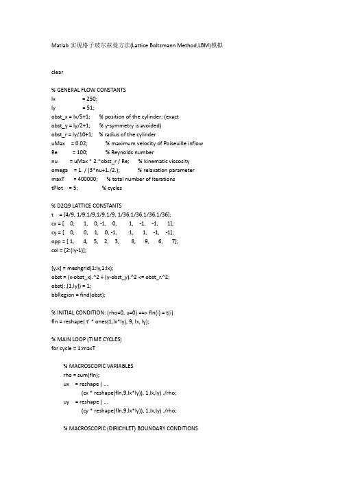
Matlab实现格子玻尔兹曼方法(Lattice Boltzmann Method,LBM)模拟clear% GENERAL FLOW CONSTANTSlx = 250;ly = 51;obst_x = lx/5+1; % position of the cylinder; (exactobst_y = ly/2+1; % y-symmetry is avoided)obst_r = ly/10+1; % radius of the cylinderuMax = 0.02; % maximum velocity of Poiseuille inflowRe = 100; % Reynolds numbernu = uMax * 2.*obst_r / Re; % kinematic viscosityomega = 1. / (3*nu+1./2.); % relaxation parametermaxT = 400000; % total number of iterationstPlot = 5; % cycles% D2Q9 LATTICE CONSTANTSt = [4/9, 1/9,1/9,1/9,1/9, 1/36,1/36,1/36,1/36];cx = [ 0, 1, 0, -1, 0, 1, -1, -1, 1];cy = [ 0, 0, 1, 0, -1, 1, 1, -1, -1];opp = [ 1, 4, 5, 2, 3, 8, 9, 6, 7];col = [2:(ly-1)];[y,x] = meshgrid(1:ly,1:lx);obst = (x-obst_x).^2 + (y-obst_y).^2 <= obst_r.^2;obst(:,[1,ly]) = 1;bbRegion = find(obst);% INITIAL CONDITION: (rho=0, u=0) ==> fIn(i) = t(i)fIn = reshape( t' * ones(1,lx*ly), 9, lx, ly);% MAIN LOOP (TIME CYCLES)for cycle = 1:maxT% MACROSCOPIC VARIABLESrho = sum(fIn);ux = reshape ( ...(cx * reshape(fIn,9,lx*ly)), 1,lx,ly) ./rho;uy = reshape ( ...(cy * reshape(fIn,9,lx*ly)), 1,lx,ly) ./rho;% MACROSCOPIC (DIRICHLET) BOUNDARY CONDITIONS% Inlet: Poiseuille profileL = ly-2; y = col-1.5;ux(:,1,col) = 4 * uMax / (L*L) * (y.*L-y.*y);uy(:,1,col) = 0;rho(:,1,col) = 1 ./ (1-ux(:,1,col)) .* ( ...sum(fIn([1,3,5],1,col)) + ...2*sum(fIn([4,7,8],1,col)) );% Outlet: Zero gradient on rho/uxrho(:,lx,col) = rho(:,lx-1,col);uy(:,lx,col) = 0;ux(:,lx,col) = ux(:,lx-1,col);% COLLISION STEPfor i=1:9cu = 3*(cx(i)*ux+cy(i)*uy);fEq(i,:,:) = rho .* t(i) .* ...( 1 + cu + 1/2*(cu.*cu) ...- 3/2*(ux.^2+uy.^2) );fOut(i,:,:) = fIn(i,:,:) - ...omega .* (fIn(i,:,:)-fEq(i,:,:));end% MICROSCOPIC BOUNDARY CONDITIONSfor i=1:9% Left boundaryfOut(i,1,col) = fEq(i,1,col) + ...18*t(i)*cx(i)*cy(i)* ( fIn(8,1,col) - ...fIn(7,1,col)-fEq(8,1,col)+fEq(7,1,col) );% Right boundaryfOut(i,lx,col) = fEq(i,lx,col) + ...18*t(i)*cx(i)*cy(i)* ( fIn(6,lx,col) - ...fIn(9,lx,col)-fEq(6,lx,col)+fEq(9,lx,col) );% Bounce back regionfOut(i,bbRegion) = fIn(opp(i),bbRegion); end% STREAMING STEPfor i=1:9fIn(i,:,:) = ...circshift(fOut(i,:,:), [0,cx(i),cy(i)]);end% VISUALIZATIONif (mod(cycle,tPlot)==0)u = reshape(sqrt(ux.^2+uy.^2),lx,ly);u(bbRegion) = nan;imagesc(u');axis equal off; drawnowendend。

格子玻尔兹曼MATLAB运用(LBGK_D2Q9_poiseuille_channel2D)

%GianniSchenaJuly2005,***************% Lattice Boltzmann LBE, geometry: D2Q9, model: BGK% Application to permeability in porous mediaRestart=false % to restart from an earlier convergencelogical(Restart);if Restart==false;close all, clear all% start from scratch and clean ...Restart=false;% type of channel geometry ;% one of the flollowing flags == truePois_test=true, % no obstacles in the 2D channel% porous systemsobs_regolare=false %obs_irregolare=false %tic% IN% |vvvv| + y% |vvvv| ^% |vvvv| | -> + x% OUT% Pores in 2D : Wet and Dry locations (Wet ==1 , Dry ==0 )wXh_Dry=[3,1];wXh_Wet=[3,4];if obs_regolare, % with internal obstaclesA=repmat([zeros(wXh_Dry),ones(wXh_Wet)],[1,3]);A=[A,zeros(wXh_Dry)];B=ones(size(A));C=[A;B] ; D=repmat(C,4,1);D=[B;D]endif obs_irregolare, % with int obstaclesA1=repmat([zeros(wXh_Dry),ones(wXh_Wet)],[1,3]);A1=[A1,zeros(wXh_Dry)] ;B=ones(size(A1));C1=repmat([ones(wXh_Wet),zeros(wXh_Dry)],[1,3]); C1=[C1,ones(wXh_Dry)]; E=[A1;B;C1;B];D=repmat(E,2,1);D=[B;D]endif ~Pois_testfigure,imshow(D,[])Channel2D=D;Len_Channel_2D=size(Channel2D,1); % LengthWidth=size(Channel2D,2); % should not be hodChannel_2D_half_Width=Width/2,end% test without obstacles (i.e. 2D channel & no obstacles)if Pois_test%over-writes the definition of the pore spaceclear Channel2DLen_Channel_2D=36, % lunghezza canale 2dChannel_2D_half_Width=8; Width=Channel_2D_half_Width*2;Channel2D=ones(Len_Channel_2D,Width); % define wet area%Channel2D(6:12,6:8)=0; % put fluid obstacleimshow(Channel2D,[]);end[Nr Mc]=size(Channel2D); % Number rows and Munber columns% porosityporosity=nnz(Channel2D==1)/(Nr*Mc)% FLUID PROPERTIES% physical propertiescs2=1/3; %cP_visco=0.5; % [cP] 1 CP Dinamic water viscosity 20 Cdensity=1.; % fluid densityLky_visco=cP_visco/density; % lattice kinematic viscosityomega=(Lky_visco/cs2+0.5).^-1; % omega: relaxation frequency%Lky_visco=cs2*(1/omega - 0.5) , % lattice kinematic viscosity%dPdL= Pressure / dL;% External pressure gradient [atm/cm]uy_fin_max=-0.2;%dPdL = abs( 2*Lky_visco*uy_fin_max/(Channel_2D_half_Width.^2) );dPdL=-0.0125;uy_fin_max=dPdL*(Channel_2D_half_Width.^2)/(2*Lky_visco); % Poiseuille Gradient;% max poiseuille final velocity on the flow profileuy0=-0.001; ux0=0.0001; % linear vel .. inizialization%% uy_fin_max=-0.2; % max poiseuille final velocity on the flow profile % omega=0.5, cs2=1/3; % omega: relaxation frequency% Lky_visco=cs2*(1/omega - 0.5) , % lattice kinematic viscosity% dPdL = abs( 2*Lky_visco*uy_fin_max/(Channel_2D_half_Width.^2) ); % Poiseuille Gradient;%uyf_av=uy_fin_max*(2/3);; % average fluid velocity on the profilex_profile=([-Channel_2D_half_Width:+Channel_2D_half_Width-1]+0.5);uy_analy_profile=uy_fin_max.*(1- ( x_profile/Channel_2D_half_Width).^2 ); % analytical velocity profileav_vel_t=1.e+10; % inizialization (t=0)%PixelSize= 5; % [Microns]%dL=(Nr*PixelSize*1.0E-4); % sample hight [cm]%% EXPERIMENTAL SET-UP% inlet and outlet buffersinb=2, oub=2; % inlet and outlet buffers thickness% add fluid at the inlet (top) and outlet (down)inlet=ones(inb,Mc); outlet=ones(oub,Mc);Channel2D=[ [inlet]; Channel2D ;[outlet] ] ; % add flux in and down (E to W)[Nr Mc]=size(Channel2D); % update size% boundaries related to the experimental set upwb=2; % wall thicknessChannel2D=[zeros(Nr,wb), Channel2D , zeros(Nr,wb)]; % add walls (no fluid leak)[Nr Mc]=size(Channel2D); % update sizeuy_analy_profile=[zeros(1,wb), uy_analy_profile, zeros(1,wb) ] ; % take into account wallsx_pro_fig=[[x_profile(1)-[wb:-1:1]], [x_profile,[1:wb]+x_profile(end)] ];% Figure plots analytical parabolic profilefigure(20), plot(x_pro_fig,uy_analy_profile,'-'), grid on,title('Analytical parab. profile for Poiseuille planar flow in a channel') % VISUALIZE PORE SPACE & FLUID OSTACLES & MEDIAL AXISfigure, imshow(Channel2D); title('Vassel geometry');Channel2D=logical(Channel2D);% obstacles for Bounce Back ( in front of the grain)Obstacles=bwperim(Channel2D,8); % perimeter of the grains for bounce back Bound.Cond.border=logical(ones(Nr,Mc));border([1:inb,Nr-oub:Nr],[wb+2:Mc-wb-1])=0;Obstacles=Obstacles.*(border);figure, imshow(Obstacles); title(' Fluid obstacles (in the fluid)' );%Medial_axis=bwmorph(Channel2D,'thin',Inf); %figure, imshow(Medial_axis); title('Medial axis');figure(10) % used to visualize evolution of rhofigure(11) % used to visualize uxfigure(12) % used to visualize uy (i.e. top -> down)% INDICES% Wet locations etc.[iabw1 jabw1]=find(Channel2D==1); % indices i,j, of active lattice locations i.e. porelena=length(iabw1); % number of active location i.e. of pore space lattice cellsija= (jabw1-1)*Nr+iabw1; % equivalent single index (i,j)->> ija for active locations% absolute (single index) position of the obstacles in for bounce back in Channel2D% Obstacles[iobs jobs]=find(Obstacles);lenobs=length(iobs); ijobs=(jobs-1)*Nr+iobs; % as above% Medial axis of the pore space[ima jma]=find(Medial_axis); lenma=length(ima); ijma= (jma-1)*Nr+ima; % as above% Internal wet locations : wet & ~obstables% (i.e. internal wet lattice location non in contact with dray locations)[iawint jawint]=find(( Channel2D==1 & ~Obstacles)); % indices i,j, of active lattice locationslenwint=length(iawint); % number of internal (i.e. not border) wet locations ijaint= (jawint-1)*Nr+iawint; % equivalent singlNxM=Nr*Mc;% DIRECTIONS: E N W S NE NW SW SE ZERO (ZERO:Rest Particle)% y^% 6 2 5 ^ NW N NE% 3 9 1 ... +x-> +y W RP E% 7 4 8 SW S SE% -y% x & y components of velocities , +x is to est , +y is to nordEast=1; North=2; West=3; South=4; NE=5; NW=6; SW=7; SE=8; RP=9;N_c=9 ; % number of directions% versors D2Q9C_x=[1 0 -1 0 1 -1 -1 1 0];C_y=[0 1 0 -1 1 1 -1 -1 0]; C=[C_x;C_y]% BOUNCE BACK SCHEME% after collision the fluid elements densities f are sent back to the% lattice node they come from with opposite direction% indices opposite to 1:8 for fast inversion after bounceic_op = [3 4 1 2 7 8 5 6]; % i.e. 4 is opposite to 2 etc.% PERIODIC BOUNDARY CONDITIONS - reinjection rulesyi2=[Nr , 1:Nr , 1]; % this definition allows implemening Period Bound Cond %yi2=[1, Nr , 2:Nr-1 , 1,Nr]; % re-inj the second last to as first% directional weights (density weights)w0=16/36. ; w1=4/36. ; w2=1/36.;W=[ w1 w1 w1 w1 w2 w2 w2 w2 w0];%c constants (sound speed related)cs2=1/3; cs2x2=2*cs2; cs4x2=2*cs2.^2;f1=1/cs2; f2=1/cs2x2; f3=1/cs4x2;f1=3., f2=4.5; f3=1.5; % coef. of the f equil.% declarative statemetsf=zeros(Nr,Mc,N_c); % array of fluid density distributionfeq=zeros(Nr,Mc,N_c); % f at equilibriumrho=ones(Nr,Mc); % macro-scopic densitytemp1=zeros(Nr,Mc);ux=zeros(Nr,Mc); uy=zeros(Nr,Mc); uyout=zeros(Nr,Mc); % dimensionless velocitiesuxsq=zeros(Nr,Mc); uysq=zeros(Nr,Mc); usq=zeros(Nr,Mc); % higher degree velocities% initialization arrays : start values in the wet areafor ia=1:lena % stat values in the active cells only ; 0 outsidei=iabw1(ia); j=jabw1(ia);f(i,j,:)=1/9; % uniform density distribution for a startenduy(ija)=uy0; ux(ija)=ux0; % initialize fluid velocitiesrho(ija)=density;% EXTERNAL (Body) FORCES e.g. inlet pressure or inlet-outlet gradient% directions: E N W S NE NW SW SE ZEROforce = -dPdL*(1/6)*1*[0 -1 0 1 -1 -1 1 1 0]'; %;%... E N E S NE NW SW SE RP ...% the pressure pushes the fluid down i.e. N to S% While .. MAIN TIME EVOLUTION LOOPStopFlag=false; % i.e. logical(0)Max_Iter=3000; % max allowed number of iterationCheck_Iter=1; Output_Every=20; % frequency of check & outputCur_Iter=0; % current iteration counter inizializationtoler=1.0e-8; % tollerance to declare convegenceCond_path=[]; % recording values of the convergence criteriumdensity_path=[]; % recording aver. density values for convergenceend% ends if restartif(Restart==true)StopFlag=false; Max_Iter=Max_Iter+3000; toler=1.0e-12;endwhile(~StopFlag)Cur_Iter=Cur_Iter+1 % iteration counter update% density and momentsrho=sum(f,3); % densityif Cur_Iter >1 % use inizialization ux uy to start% Moments ... Note:C_x(9)=C_y(9)=0ux=zeros(Nr,Mc); uy=zeros(Nr,Mc);for ic=1:N_c-1;ux = ux + C_x(ic).*f(:,:,ic) ; uy = uy + C_y(ic).*f(:,:,ic) ;end% uy=f(:,:,2) +f(:,:,5)+f(:,:,6)-f(:,:,4)-f(:,:,7)-f(:,:,8); % in short !% ux=f(:,:,1) +f(:,:,5)+f(:,:,8)-f(:,:,3)-f(:,:,6)-f(:,:,7); % in short !end%%%%%%%%%%%%%%%%%%%%%%%%%%%%%%%%%%%%%%%%%%%%%%%%%%%%%%%%%%%%%ux(ija)=ux(ija)./rho(ija); uy(ija)=uy(ija)./rho(ija);uxsq(ija)=ux(ija).^2; uysq(ija)=uy(ija).^2;usq(ija)=uxsq(ija)+uysq(ija); %% weighted densities : rest particle, principal axis, diagonalsrt0 = w0.*rho; rt1 = w1.*rho; rt2 = w2.*rho;% Equilibrium distribution% main directions ( + cross)feq(ija)= rt1(ija) .*(1 +f1*ux(ija) +f2*uxsq(ija) -f3*usq(ija));feq(ija+NxM*(2-1))= rt1(ija) .*(1 +f1*uy(ija) +f2*uysq(ija)-f3*usq(ija));feq(ija+NxM*(3-1))= rt1(ija) .*(1 -f1*ux(ija) +f2*uxsq(ija)-f3*usq(ija));%feq(ija+NxM*(3)=f(ija)-2*rt1(ija)*f1.*ux(ija); % much faster... !! feq(ija+NxM*(4-1))= rt1(ija) .*(1 -f1*uy(ija) +f2*uysq(ija)-f3*usq(ija));% diagonals (X diagonals) (ic-1)feq(ija+NxM*(5-1))= rt2(ija) .*(1 +f1*(+ux(ija)+uy(ija))+f2*(+ux(ija)+uy(ija)).^2 -f3.*usq(ija));feq(ija+NxM*(6-1))= rt2(ija) .*(1 +f1*(-ux(ija)+uy(ija))+f2*(-ux(ija)+uy(ija)).^2 -f3.*usq(ija));feq(ija+NxM*(7-1))= rt2(ija) .*(1 +f1*(-ux(ija)-uy(ija))+f2*(-ux(ija)-uy(ija)).^2 -f3.*usq(ija));feq(ija+NxM*(8-1))= rt2(ija) .*(1 +f1*(+ux(ija)-uy(ija))+f2*(+ux(ija)-uy(ija)).^2 -f3.*usq(ija));% rest particle (.) ic=9feq(ija+NxM*(9-1))= rt0(ija) .*(1 - f3*usq(ija));%Collision (between fluid elements)omega=relaxation frequencyf=(1.-omega).*f + omega.*feq;%%%%%%%%%%%%%%%%%%%%%%%%%%%%%%%%%%%%%%%%%%%%%%%%%%%%%%%%%%add external body force due to the pressure gradient prop. to dPdL for ic=1:N_c;%-1for ia=1:lenai=iabw1(ia); j=jabw1(ia);% if Obstacles(i,j)==0 % the i,j is not aderent to the boundaries% if ( f(i,j,ic) + force(ic) ) >0; %! avoid negative distributions%i=1 ;% force only on the first row !f(i,j,ic)= f(i,j,ic) + force(ic);% end% endendend% % STREAM% Forward Propagation step & % Bounce Back (collision fluid with obstacles) %f(:,:,9) = f(:,:,9); % Rest element do not movefeq = f; % temp storage of f in feqfor ic=1:1:N_c-1, % select velocity layeric2=ic_op(ic); % selects the layer of the velocity opposite to ic for BBtemp1=feq(:,:,ic); %% from wet location that are NOT on the border to other wet locationsfor ia=1:1:lenwint % number of internal (i.e. not border) wet locations i=iawint(ia); j=jawint(ia); % so that we care for the wet space only !i2 = i+C_y(ic); j2 = j+C_x(ic); % Expected final locations to move i2=yi2(i2+1); % i2 corrected for PBC when necessary (flow out re-fed to inlet)% i.e the new position (i2,j2) is sure another wet location% therefore normal propagation from (i,j) to (i2,j2) on layer ic f(i2,j2,ic)=temp1(i,j); % see circshift(..) fnct for circularly shiftsend ; % i and j single loop% from wet locations that ARE on the border of obstaclesfor ia=1:1:lenobs % wet border locationsi=iobs(ia); j=jobs(ia); % so that we care for the wet space only ! i2 = i+C_y(ic); j2 = j+C_x(ic); % Expected final locations to move i2=yi2(i2+1); % i2 corrected for PBCif( Channel2D(i2,j2) ==0 ) % i.e the new position (i2,j2) is dry f(i,j,ic2) =temp1(i,j); % invert direction: bounce-back in the opposite direction ic2else% otherwise, normal propagation from (i,j) to (i2,j2) on layer icf(i2,j2,ic)=temp1(i,j); % see circshift(..) fnct for circularly shiftsend ; % b.b. and propagationsend ; % i and j single loop% special treatment for Corners% f(1,wb+1,ic)=temp1(Nr,Mc-wb);f(1,Mc-wb,ic)=temp1(Nr,wb+1);% f(Nr,wb+1,ic)=temp1(1,Mc-wb);f(Nr,Mc-wb,ic)=temp1(1,wb+1);end ; % for ic direction% ends of Forward Propagation step & Bounce Back Sections% re-calculate uy as uyout for convergencerho=sum(f,3); % density% check velocityuyout= zeros(Nr,Mc);for ic=1:N_c-1;uyout= uyout + C_y(ic).*f(:,:,ic) ; % flow dim.less velocity out end% uyout(ija)=uyout(ija)./rho(ija); % from momentum to velocity% Convergence check on velocity valuesif (mod(Cur_Iter,Check_Iter)==0) ; % check for convergence every'Check_Iter' iterations% variables monitored% mean density andvect=rho(ija); vect=vect(:);cur_density=mean(vect);% mean 'interstitial' velocity% uy(ija)=uy(ija)/rho(ija); ?vect=uy(ija); av_vel_int= mean(vect) ; % seepage velocity (in the wet area)% on the whole cross-sectional area of flow (wet + dry)av_vel_int=av_vel_int*porosity, % av. vel. on the wet + dry area %av_vel_int=mean2(uy),av_vel_tp1 = av_vel_int;Condition=abs( abs(av_vel_t/av_vel_tp1 )-1), % should --> 0Cond_path=[Cond_path, Condition]; % records the convergence path (value)density_path=[density_path, cur_density];%av_vel_t=av_vel_tp1; % time t & t+1if (Condition < toler) | (Cur_Iter > Max_Iter)StopFlag=true;display( 'Stop iteration: Convergence met or iteration exeeding the max allowed' )display( ['Current iteration: ',num2str(Cur_Iter),...' Max Number of iter: ',num2str(Max_Iter)] )break% Terminate execution of WHILE .. exit the time evolution loop.end% if(Condition < tolerendif (mod(Cur_Iter,Output_Every)==0) ; % Output from loop every ...%if (Cur_Iter>60) ; % Output from loop every ...rho=sum(f,3); % densityfigure(10); imshow(rho,[0.1 0.9]); title(' rho'); % visualize density evolutionfigure(11); imshow(ux,[ ]); title(' ux'); % visualize fluid velocity horizontalfigure(12); imshow(-uy,[ ]); title(' uy'); % visualize fluid velocity downfigure(14), imshow(-uyout,[]), title('uyout'); % vis vel flow out up=2; % linear section to visualize up from the lower rowfigure(15), hold off, feather(ux(Nr-up,:),uy(Nr-up,:)),figure(15), hold on , plot(uy_analy_profile,'r-')title('Analytical vs LB calculated, fluid velocity parabolicprofile')pause(3); % time given to visualize properlyend% every% pause(1);end% End main time Evolution Loop% Output & Draw after the end of the time evolutionfigure, plot(Cond_path(2:end)); title('convergence path')%figure, plot(density_path(2:end)); title('density convergence path') figure, plot( [uy(Nr-up,:)-uy_analy_profile] ); title('difference : LB - Analytical solution')toc% Permeability KK_Darcy_Porous_Sys= (av_vel_int*porosity)/dPdL*Lky_visco , K_Analy_2D_Channel=(Width^2)/12。

格子玻尔兹曼算法

格子玻尔兹曼算法
格子玻尔兹曼算法是一种基于微观粒子运动的计算流体力学方法，它可以用来模拟流体的运动和传输过程。

该算法的核心思想是将流体分成许多小的格子，然后在每个格子内模拟流体粒子的运动和相互作用，从而得到整个流体的宏观运动状态。

格子玻尔兹曼算法的基本原理是通过离散化的方式来模拟流体的微观运动。

在每个格子内，流体粒子的运动状态可以用一个分布函数来描述，该函数包含了流体粒子在不同速度下的密度和速度信息。

通过对分布函数的离散化和更新，可以得到流体的宏观运动状态，如速度、密度和压力等。

格子玻尔兹曼算法的优点是可以处理复杂的流体运动和传输过程，如湍流、多相流和热传导等。

同时，该算法具有高效、可扩展和易于并行化等特点，可以在大规模计算机集群上进行高性能计算。

然而，格子玻尔兹曼算法也存在一些挑战和限制。

首先，该算法需要对流体的微观运动进行离散化，因此需要选择合适的离散化方法和参数，以保证模拟结果的准确性和稳定性。

其次，该算法需要进行大量的计算和存储，因此需要高性能计算机和存储系统的支持。

最后，该算法在处理复杂流体问题时，需要考虑多种物理过程的相互作用，因此需要进行多物理场的耦合和协同计算。

格子玻尔兹曼算法是一种重要的计算流体力学方法，它可以用来模
拟各种复杂的流体运动和传输过程。

随着计算机技术的不断发展和进步，该算法将在更广泛的领域得到应用和发展。

格子boltzmann方法的理论及应用

格子boltzmann方法的理论及应用
格子波尔兹曼方法(Grid Boltzmann Method, GBM)是一种非离散化处理方法，其基本
思想是在空间上采用格点，并建立格点微分方程组来解决复杂流体或者其他相关物理问题. GBM以较少的计算量就可达到快速、精确求解流体动力学问题，而且将空间和时间分离，
大大减少计算量和存储量，可以说是比传统有限元技术和有限差分技术更加有效的一种方法.
格子波尔兹曼方法的具体原理是：格子波尔兹曼方法是将空间上的解释解划分成一系
列的蒙特卡洛格子点，这样可以以非离散化处理。

针对与流体物理仿真相关的变量，以格
点位置为基底，可以使用波尔兹曼分布Y(v)来描述，将原本复杂的多体相互作用模型转化为简单的蒙特卡洛定值模型，由此通过空间离散的方式可以求解波尔兹曼方程；具体的应
用也很广泛，可以应用在流体动力学中，可用来模拟很多液体问题，比如湍流传播和燃烧
等方面；在地形风化中可以用来模拟流域洪水演变和地形演化、土壤流失问题；在水质污
染领域，可以用来模拟河流污染物质运行规律；在非牛顿流体中，可用来模拟非牛顿流体
动力学问题；在金属粒子、微粒或者多组分液体中，可用来模拟粒子间相互作用，甚至可
以应用在非弹性波中进行数值模拟.
格子波尔兹曼方法因其独特的优越性深受广泛重视，在国内外都有大量的研究，结合
其他的数值方法，用于模拟复杂的流体物理系统，改善计算效率，提高建模的准确性。

GBM具有更快的计算速度和精度优势，在现代的科学技术领域有着广泛的应用，如流体动
力学，地形风化，水质污染等问题。

该方法不仅可用作模拟计算复杂流体运动，而且可以
用于半定常及强力学分析中。

格子波尔兹曼方法

格子波尔兹曼方法是一种用于表示动力学系统的数值求解方法，由波
尔兹曼在1945年提出。

该方法可以用来模拟复杂的非线性动力学系统，在物理学、电子学、数学等领域都有着广泛的应用。

格子波尔兹曼方法是常微分方程计算的一种数值方法，可以用于多元
常微分方程。

该方法是把一个描述某力学系统的多元常微分方程组，
分别代入单元函数，离散化格点，细分各个区间；然后求解出这一系
统的运动规律。

为了能够计算出更加精准的结果，在计算中应使用尽
可能小的初始粒子，这样就能更好地模拟出真实的物理现象。

除了可以用于计算多元常微分方程的格子波尔兹曼方法外，它还可用
于计算经典力学下的库伦方程组。

库伦方程是一种解析由动量守恒定
律推出的动能方程，当研究的物体有一定的变形时，就不能得到准确
的解。

在这种情况下，就可以使用格子波尔兹曼方法来求解库伦方程，以更准确地模拟物体的运动。

格子波尔兹曼方法广泛应用于物理学和工程学，尤其是在计算多元常
微分方程和库伦方程组时推广。

它可以用来模拟微观结构系统的动力学，如粒子系统和空气动力学，也可以用于流体力学，热力学，电磁
学等。

此外，格子波尔兹曼方法也可以用于解决由非线性未知依赖性
的复杂动力学系统。

总之，格子波尔兹曼方法在物理和工程领域十分重要，在不断求精的
工作中减少了模型的复杂度，使推理和计算更加精确，为工程人员提
供了一种新的建模方式。

玻尔兹曼方程的蒙特卡洛模拟matlab

一、介绍玻尔兹曼方程及其意义玻尔兹曼方程是描述气体分子运动和统计力学行为的基本方程之一，它被广泛应用于研究气体动力学、等离子体物理学和流体力学等领域。

玻尔兹曼方程可以用来描述气体分子在外力和碰撞作用下的运动状态和分布规律，是建立气体动力学理论模型和计算模拟的重要基础。

二、玻尔兹曼方程的蒙特卡洛模拟原理蒙特卡洛方法是一种基于随机抽样的计算模拟方法，它通过大量的随机抽样实验来逼近复杂系统的统计特性和行为规律。

在玻尔兹曼方程的模拟研究中，蒙特卡洛方法可以被应用于模拟气体分子的运动轨迹、碰撞行为和能量传递过程，从而得到气体的动力学特性和统计规律。

三、利用matlab进行玻尔兹曼方程的蒙特卡洛模拟在实际研究中，matlab作为一种强大的科学计算和数值模拟软件，可以被广泛用于玻尔兹曼方程的蒙特卡洛模拟研究。

利用matlab编程，可以实现气体分子的随机运动模拟、碰撞过程模拟和能量转移模拟，从而得到气体力学性质和统计规律的数值模拟结果。

四、matlab编程实现玻尔兹曼方程的蒙特卡洛模拟方法1. 确定气体分子的初始位置和速度分布，随机生成气体分子的初始状态参数。

2. 设置气体分子的运动模拟范围和时间步长，确定模拟的时间和空间尺度。

3. 根据玻尔兹曼方程的碰撞积分表达式和分布函数表达式，编写碰撞模拟和分布函数更新的数值计算代码。

4. 建立气体分子的碰撞模拟和能量转移模拟模型，编写碰撞判定和动量能量转移的数值模拟算法。

5. 进行玻尔兹曼方程的蒙特卡洛模拟计算，得到气体分子的运动轨迹和分布规律的数值模拟结果。

6. 分析和解释模拟结果，得到气体力学性质和统计规律的数值模拟结论。

五、matlab实例代码示例```matlab确定模拟参数N = 1000; 气体分子数L = 10; 模拟尺度t = 100; 模拟时间初始化气体分子状态pos = rand(N, 3) * L; 随机生成气体分子的初始位置vel = randn(N, 3); 随机生成气体分子的初始速度模拟气体分子的运动和碰撞for i = 1:t更新气体分子的位置和速度pos = pos + vel; 更新气体分子的位置vel = vel + randn(N, 3) * 0.1; 模拟气体分子的随机运动检测气体分子的碰撞idx = detect_collision(pos, L); 判定气体分子的碰撞vel(idx, :) = -vel(idx, :); 碰撞反弹end分析模拟结果统计气体分子的分布规律和能量特性```六、总结与展望玻尔兹曼方程的蒙特卡洛模拟是一种重要的研究方法，它可以帮助研究人员理解气体动力学和统计力学行为，并且可以为气体流体力学和等离子体物理学等领域的研究提供重要的数值模拟支持。

受限玻尔兹曼机matlab实现

受限玻尔兹曼机（Restricted Boltzmann Machine）的介绍与实现1. 什么是受限玻尔兹曼机受限玻尔兹曼机（Restricted Boltzmann Machine，简称RBM）是一种基于概率模型的人工神经网络，属于无监督学习算法。

它由一个可见层和一个隐藏层组成，可用于对数据进行特征提取、降维、生成模型等任务。

RBM的结构简单、训练高效，并且在很多领域都取得了成功应用。

RBM的核心思想是通过最大化数据的似然函数来学习模型参数。

其基本原理和数学推导可以参考相关文献和论文。

在本文中，我们将重点介绍如何使用Matlab实现一个简单的受限玻尔兹曼机。

2. 受限玻尔兹曼机的实现步骤2.1 数据预处理在开始实现之前，我们需要对输入数据进行预处理。

通常情况下，我们会将输入数据进行归一化处理，使其数值范围在0到1之间。

2.2 初始化模型参数RBM的模型参数包括可见层与隐藏层之间的权重矩阵W、可见层与隐藏层的偏置向量b和c。

我们可以使用随机数生成器来初始化这些参数。

num_visible_units = size(data, 2); % 可见层神经元数量num_hidden_units = 100; % 隐藏层神经元数量W = randn(num_visible_units, num_hidden_units); % 初始化权重矩阵b = zeros(1, num_visible_units); % 初始化可见层偏置向量c = zeros(1, num_hidden_units); % 初始化隐藏层偏置向量2.3 训练模型RBM的训练过程通常使用对比散度（Contrastive Divergence）算法，它是一种近似最大似然估计方法。

训练过程包括两个阶段：正向传播和反向传播。

正向传播正向传播是指从可见层到隐藏层的信息传递过程。

在正向传播时，我们首先计算隐藏层的激活概率，并根据激活概率生成隐藏层的状态。

流体动力学的格子boltzmann方法及其具体实现

流体动力学的格子boltzmann方法及其具体实现格子Boltzmann方法是以Boltzmann方程为基础的，该方程描述了流体中粒子的运动。

格子Boltzmann方法将模拟的流体区域划分为一个个离散的格子，并在每个格子中表示流体的宏观属性，如密度、速度等。

在每个格子中，通过计算碰撞和分布函数来模拟粒子的运动。

具体实现格子Boltzmann方法的步骤如下：1.离散化：首先，将流体区域离散化为一个个格子。

格子的大小可以根据需要进行调整。

2.分布函数：在每个格子中，引入分布函数来描述粒子的密度和速度。

分布函数是一个概率密度函数，表示在给定位置和速度的条件下，粒子在该位置具有该速度的概率。

3.碰撞模拟：在每个格子中，模拟粒子之间的碰撞。

根据碰撞模型，计算粒子之间的相互作用，并更新分布函数。

4.传输：根据速度和分布函数，计算粒子的传输过程。

传输过程描述了粒子从一个格子到另一个格子的流动。

5.边界条件：在模拟流体区域的边界上，需要设置适当的边界条件。

边界条件可以影响流体的流动模式。

6.时间步进：通过迭代计算，不断更新格子中的分布函数。

每个时间步长都对应着碰撞和传输的过程。

格子Boltzmann方法与其他常用的计算流体力学方法相比具有一些优势：1. 高效性：格子Boltzmann方法使用离散化格子的方式来模拟流体运动，计算量相对较小，能够高效地处理大规模流体问题。

2. 并行性：由于格子Boltzmann方法的计算是在各个格子之间进行的，因此可以方便地实现并行计算，利用多核处理器或分布式计算系统，加速计算速度。

3. 多尺度：格子Boltzmann方法可以在不同的尺度上进行模拟，从宏观的流体行为到微观的分子动力学。

4. 可分析性：格子Boltzmann方法建立在Boltzmann方程的基础上，可以通过对方程的分析来推导流体的宏观行为。

总结而言，格子Boltzmann方法是一种基于离散化格子的流体动力学模拟方法，通过计算碰撞和传输过程来模拟流体的运动。

【VIP专享】格子玻尔兹曼MATLAB运用(LBGK_D2Q9_poiseuille_channel2D)

% Gianni Schena July 2005, schena@units.it% Lattice Boltzmann LBE, geometry: D2Q9, model: BGK% Application to permeability in porous mediaRestart=false % to restart from an earlier convergencelogical(Restart);if Restart==false;close all, clear all% start from scratch and clean ...Restart=false;% type of channel geometry ;% one of the flollowing flags == truePois_test=true, % no obstacles in the 2D channel% porous systemsobs_regolare=false %obs_irregolare=false %tic% IN% |vvvv| + y% |vvvv| ^% |vvvv| | -> + x% OUT% Pores in 2D : Wet and Dry locations (Wet ==1 , Dry ==0 )wXh_Dry=[3,1];wXh_Wet=[3,4];if obs_regolare, % with internal obstaclesA=repmat([zeros(wXh_Dry),ones(wXh_Wet)],[1,3]);A=[A,zeros(wXh_Dry)];B=ones(size(A));C=[A;B] ; D=repmat(C,4,1);D=[B;D]endif obs_irregolare, % with int obstaclesA1=repmat([zeros(wXh_Dry),ones(wXh_Wet)],[1,3]);A1=[A1,zeros(wXh_Dry)] ;B=ones(size(A1));C1=repmat([ones(wXh_Wet),zeros(wXh_Dry)],[1,3]); C1=[C1,ones(wXh_Dry)]; E=[A1;B;C1;B];D=repmat(E,2,1);D=[B;D]endif ~Pois_testfigure,imshow(D,[])Channel2D=D;Len_Channel_2D=size(Channel2D,1); % LengthWidth=size(Channel2D,2); % should not be hodChannel_2D_half_Width=Width/2,end% test without obstacles (i.e. 2D channel & no obstacles)if Pois_test%over-writes the definition of the pore spaceclear Channel2DLen_Channel_2D=36, % lunghezza canale 2dChannel_2D_half_Width=8; Width=Channel_2D_half_Width*2;Channel2D=ones(Len_Channel_2D,Width); % define wet area%Channel2D(6:12,6:8)=0; % put fluid obstacleimshow(Channel2D,[]);end[Nr Mc]=size(Channel2D); % Number rows and Munber columns% porosityporosity=nnz(Channel2D==1)/(Nr*Mc)% FLUID PROPERTIES% physical propertiescs2=1/3; %cP_visco=0.5; % [cP] 1 CP Dinamic water viscosity 20 Cdensity=1.; % fluid densityLky_visco=cP_visco/density; % lattice kinematic viscosityomega=(Lky_visco/cs2+0.5).^-1; % omega: relaxation frequency%Lky_visco=cs2*(1/omega - 0.5) , % lattice kinematic viscosity%dPdL= Pressure / dL;% External pressure gradient [atm/cm]uy_fin_max=-0.2;%dPdL = abs( 2*Lky_visco*uy_fin_max/(Channel_2D_half_Width.^2) );dPdL=-0.0125;uy_fin_max=dPdL*(Channel_2D_half_Width.^2)/(2*Lky_visco); % Poiseuille Gradient;% max poiseuille final velocity on the flow profileuy0=-0.001; ux0=0.0001; % linear vel .. inizialization%% uy_fin_max=-0.2; % max poiseuille final velocity on the flow profile % omega=0.5, cs2=1/3; % omega: relaxation frequency% Lky_visco=cs2*(1/omega - 0.5) , % lattice kinematic viscosity% dPdL = abs( 2*Lky_visco*uy_fin_max/(Channel_2D_half_Width.^2) ); % Poiseuille Gradient;%uyf_av=uy_fin_max*(2/3);; % average fluid velocity on the profilex_profile=([-Channel_2D_half_Width:+Channel_2D_half_Width-1]+0.5);uy_analy_profile=uy_fin_max.*(1- ( x_profile /Channel_2D_half_Width).^2 ); % analytical velocity profileav_vel_t=1.e+10; % inizialization (t=0)%PixelSize= 5; % [Microns]%dL=(Nr*PixelSize*1.0E-4); % sample hight [cm]%% EXPERIMENTAL SET-UP% inlet and outlet buffersinb=2, oub=2; % inlet and outlet buffers thickness% add fluid at the inlet (top) and outlet (down)inlet=ones(inb,Mc); outlet=ones(oub,Mc);Channel2D=[ [inlet]; Channel2D ;[outlet] ] ; % add flux in and down (E to W)[Nr Mc]=size(Channel2D); % update size% boundaries related to the experimental set upwb=2; % wall thicknessChannel2D=[zeros(Nr,wb), Channel2D , zeros(Nr,wb)]; % add walls (nofluid leak)[Nr Mc]=size(Channel2D); % update sizeuy_analy_profile=[zeros(1,wb), uy_analy_profile, zeros(1,wb) ] ; % take into account wallsx_pro_fig=[[x_profile(1)-[wb:-1:1]], [x_profile, [1:wb]+x_profile(end)] ];% Figure plots analytical parabolic profilefigure(20), plot(x_pro_fig,uy_analy_profile,'-'), grid on,title('Analytical parab. profile for Poiseuille planar flow in achannel')% VISUALIZE PORE SPACE & FLUID OSTACLES & MEDIAL AXISfigure, imshow(Channel2D); title('Vassel geometry');Channel2D=logical(Channel2D);% obstacles for Bounce Back ( in front of the grain)Obstacles=bwperim(Channel2D,8); % perimeter of the grains for bounce back Bound.Cond.border=logical(ones(Nr,Mc));border([1:inb,Nr-oub:Nr],[wb+2:Mc-wb-1])=0;Obstacles=Obstacles.*(border);figure, imshow(Obstacles); title(' Fluid obstacles (in the fluid)' );%Medial_axis=bwmorph(Channel2D,'thin',Inf); %figure, imshow(Medial_axis); title('Medial axis');figure(10) % used to visualize evolution of rhofigure(11) % used to visualize uxfigure(12) % used to visualize uy (i.e. top -> down)% INDICES% Wet locations etc.[iabw1 jabw1]=find(Channel2D==1); % indices i,j, of active lattice locations i.e. porelena=length(iabw1); % number of active location i.e. of pore spacelattice cellsija= (jabw1-1)*Nr+iabw1; % equivalent single index (i,j)->> ija for active locations% absolute (single index) position of the obstacles in for bounce back in Channel2D% Obstacles[iobs jobs]=find(Obstacles);lenobs=length(iobs); ijobs= (jobs-1)*Nr+iobs; % as above% Medial axis of the pore space[ima jma]=find(Medial_axis); lenma=length(ima); ijma= (jma-1)*Nr+ima; % as above% Internal wet locations : wet & ~obstables% (i.e. internal wet lattice location non in contact with dray locations)[iawint jawint]=find(( Channel2D==1 & ~Obstacles)); % indices i,j, of active lattice locationslenwint=length(iawint); % number of internal (i.e. not border) wet locationsijaint= (jawint-1)*Nr+iawint; % equivalent singlNxM=Nr*Mc;% DIRECTIONS: E N W S NE NW SW SE ZERO (ZERO:Rest Particle)% y^% 6 2 5 ^ NW N NE% 3 9 1 ... +x-> +y W RP ESW S SE% 7 4 8% -y% x & y components of velocities , +x is to est , +y is to nordEast=1; North=2; West=3; South=4; NE=5; NW=6; SW=7; SE=8; RP=9;N_c=9 ; % number of directions% versors D2Q9C_x=[1 0 -1 0 1 -1 -1 1 0];C_y=[0 1 0 -1 1 1 -1 -1 0]; C=[C_x;C_y]% BOUNCE BACK SCHEME% after collision the fluid elements densities f are sent back to the% lattice node they come from with opposite direction% indices opposite to 1:8 for fast inversion after bounceic_op = [3 4 1 2 7 8 5 6]; % i.e. 4 is opposite to 2 etc.% PERIODIC BOUNDARY CONDITIONS - reinjection rulesyi2=[Nr , 1:Nr , 1]; % this definition allows implemening Period Bound Cond%yi2=[1, Nr , 2:Nr-1 , 1,Nr]; % re-inj the second last to as first% directional weights (density weights)w0=16/36. ; w1=4/36. ; w2=1/36.;W=[ w1 w1 w1 w1 w2 w2 w2 w2 w0];%c constants (sound speed related)cs2=1/3; cs2x2=2*cs2; cs4x2=2*cs2.^2;f1=1/cs2; f2=1/cs2x2; f3=1/cs4x2;f1=3., f2=4.5; f3=1.5; % coef. of the f equil.% declarative statemetsf=zeros(Nr,Mc,N_c); % array of fluid density distributionfeq=zeros(Nr,Mc,N_c); % f at equilibriumrho=ones(Nr,Mc); % macro-scopic densitytemp1=zeros(Nr,Mc);ux=zeros(Nr,Mc); uy=zeros(Nr,Mc); uyout=zeros(Nr,Mc); % dimensionless velocitiesuxsq=zeros(Nr,Mc); uysq=zeros(Nr,Mc); usq=zeros(Nr,Mc); % higher degree velocities% initialization arrays : start values in the wet areafor ia=1:lena % stat values in the active cells only ; 0 outside i=iabw1(ia); j=jabw1(ia);f(i,j,:)=1/9; % uniform density distribution for a startenduy(ija)=uy0; ux(ija)=ux0; % initialize fluid velocitiesrho(ija)=density;% EXTERNAL (Body) FORCES e.g. inlet pressure or inlet-outlet gradient% directions: E N W S NE NW SW SE ZEROforce = -dPdL*(1/6)*1*[0 -1 0 1 -1 -1 1 1 0]'; %;E N E S NE NW SW SE RP ...%...% the pressure pushes the fluid down i.e. N to S% While .. MAIN TIME EVOLUTION LOOPStopFlag=false; % i.e. logical(0)Max_Iter=3000; % max allowed number of iterationCheck_Iter=1; Output_Every=20; % frequency of check & outputCur_Iter=0; % current iteration counter inizializationtoler=1.0e-8; % tollerance to declare convegenceCond_path=[]; % recording values of the convergence criteriumdensity_path=[]; % recording aver. density values for convergenceend% ends if restartif(Restart==true)StopFlag=false; Max_Iter=Max_Iter+3000; toler=1.0e-12;endwhile(~StopFlag)Cur_Iter=Cur_Iter+1 % iteration counter update% density and momentsrho=sum(f,3); % densityif Cur_Iter >1 % use inizialization ux uy to start% Moments ... Note:C_x(9)=C_y(9)=0ux=zeros(Nr,Mc); uy=zeros(Nr,Mc);for ic=1:N_c-1;ux = ux + C_x(ic).*f(:,:,ic) ; uy = uy + C_y(ic).*f(:,:,ic) ;end% uy=f(:,:,2) +f(:,:,5)+f(:,:,6)-f(:,:,4)-f(:,:,7)-f(:,:,8); % in short !% ux=f(:,:,1) +f(:,:,5)+f(:,:,8)-f(:,:,3)-f(:,:,6)-f(:,:,7); % in short !end%%%%%%%%%%%%%%%%%%%%%%%%%%%%%%%%%%%%%%%%%%%%%%%%%%%%%%%%%%%%%ux(ija)=ux(ija)./rho(ija); uy(ija)=uy(ija)./rho(ija);uxsq(ija)=ux(ija).^2; uysq(ija)=uy(ija).^2;usq(ija)=uxsq(ija)+uysq(ija); %% weighted densities : rest particle, principal axis, diagonalsrt0 = w0.*rho; rt1 = w1.*rho; rt2 = w2.*rho;% Equilibrium distribution% main directions ( + cross)feq(ija)= rt1(ija) .*(1 +f1*ux(ija) +f2*uxsq(ija) -f3*usq(ija));feq(ija+NxM*(2-1))= rt1(ija) .*(1 +f1*uy(ija) +f2*uysq(ija) -f3*usq(ija));feq(ija+NxM*(3-1))= rt1(ija) .*(1 -f1*ux(ija) +f2*uxsq(ija) -f3*usq(ija));%feq(ija+NxM*(3)=f(ija)-2*rt1(ija)*f1.*ux(ija); % much faster... !!feq(ija+NxM*(4-1))= rt1(ija) .*(1 -f1*uy(ija) +f2*uysq(ija) -f3*usq(ija));% diagonals (X diagonals) (ic-1)feq(ija+NxM*(5-1))= rt2(ija) .*(1 +f1*(+ux(ija)+uy(ija))+f2*(+ux(ija)+uy(ija)).^2 -f3.*usq(ija));feq(ija+NxM*(6-1))= rt2(ija) .*(1 +f1*(-ux(ija)+uy(ija)) +f2*(-ux(ija)+uy(ija)).^2 -f3.*usq(ija));feq(ija+NxM*(7-1))= rt2(ija) .*(1 +f1*(-ux(ija)-uy(ija)) +f2*(-ux(ija)-uy(ija)).^2 -f3.*usq(ija));feq(ija+NxM*(8-1))= rt2(ija) .*(1 +f1*(+ux(ija)-uy(ija))+f2*(+ux(ija)-uy(ija)).^2 -f3.*usq(ija));% rest particle (.) ic=9feq(ija+NxM*(9-1))= rt0(ija) .*(1 - f3*usq(ija));%Collision (between fluid elements)omega=relaxation frequencyf=(1.-omega).*f + omega.*feq;%%%%%%%%%%%%%%%%%%%%%%%%%%%%%%%%%%%%%%%%%%%%%%%%%%%%%%%%%%add external body force due to the pressure gradient prop. to dPdL for ic=1:N_c;%-1for ia=1:lenai=iabw1(ia); j=jabw1(ia);% if Obstacles(i,j)==0 % the i,j is not aderent to the boundaries% if ( f(i,j,ic) + force(ic) ) >0; %! avoid negative distributions%i=1 ;% force only on the first row !f(i,j,ic)= f(i,j,ic) + force(ic);% end% endendend% % STREAM% Forward Propagation step & % Bounce Back (collision fluid with obstacles)%f(:,:,9) = f(:,:,9); % Rest element do not movefeq = f; % temp storage of f in feqfor ic=1:1:N_c-1, % select velocity layeric2=ic_op(ic); % selects the layer of the velocity opposite to ic for BBtemp1=feq(:,:,ic); %% from wet location that are NOT on the border to other wet locationsfor ia=1:1:lenwint % number of internal (i.e. not border) wet locationsi=iawint(ia); j=jawint(ia); % so that we care for the wetspace only !i2 = i+C_y(ic); j2 = j+C_x(ic); % Expected final locations to movei2=yi2(i2+1); % i2 corrected for PBC when necessary (flow out re-fed to inlet)% i.e the new position (i2,j2) is sure another wet location% therefore normal propagation from (i,j) to (i2,j2) on layer icf(i2,j2,ic)=temp1(i,j); % see circshift(..) fnct forcircularly shiftsend ; % i and j single loop% from wet locations that ARE on the border of obstaclesfor ia=1:1:lenobs % wet border locationsi=iobs(ia); j=jobs(ia); % so that we care for the wet space only !i2 = i+C_y(ic); j2 = j+C_x(ic); % Expected final locations to movei2=yi2(i2+1); % i2 corrected for PBCif( Channel2D(i2,j2) ==0 ) % i.e the new position (i2,j2) is dryf(i,j,ic2) =temp1(i,j); % invert direction: bounce-back in the opposite direction ic2else% otherwise, normal propagation from (i,j) to (i2,j2) on layer icf(i2,j2,ic)=temp1(i,j); % see circshift(..) fnct for circularly shiftsend ; % b.b. and propagationsend ; % i and j single loop% special treatment for Corners% f(1,wb+1,ic)=temp1(Nr,Mc-wb); f(1,Mc-wb,ic)=temp1(Nr,wb+1);% f(Nr,wb+1,ic)=temp1(1,Mc-wb); f(Nr,Mc-wb,ic)=temp1(1,wb+1);end ; % for ic direction% ends of Forward Propagation step & Bounce Back Sections% re-calculate uy as uyout for convergencerho=sum(f,3); % density% check velocityuyout= zeros(Nr,Mc);for ic=1:N_c-1;uyout= uyout + C_y(ic).*f(:,:,ic) ; % flow dim.less velocity out end% uyout(ija)=uyout(ija)./rho(ija); % from momentum to velocity% Convergence check on velocity valuesif (mod(Cur_Iter,Check_Iter)==0) ; % check for convergence every'Check_Iter' iterations% variables monitored% mean density andvect=rho(ija); vect=vect(:);cur_density=mean(vect);% mean 'interstitial' velocity% uy(ija)=uy(ija)/rho(ija); ?vect=uy(ija); av_vel_int= mean(vect) ; % seepage velocity (in the wet area)% on the whole cross-sectional area of flow (wet + dry)av_vel_int=av_vel_int*porosity, % av. vel. on the wet + dry area%av_vel_int=mean2(uy),av_vel_tp1 = av_vel_int;Condition=abs( abs(av_vel_t/av_vel_tp1 )-1), % should --> 0Cond_path=[Cond_path, Condition]; % records the convergence path (value)density_path=[density_path, cur_density];%av_vel_t=av_vel_tp1; % time t & t+1if (Condition < toler) | (Cur_Iter > Max_Iter)StopFlag=true;display( 'Stop iteration: Convergence met or iteration exeeding the max allowed' )display( ['Current iteration: ',num2str(Cur_Iter),...' Max Number of iter: ',num2str(Max_Iter)] )break% Terminate execution of WHILE .. exit the time evolution loop.end% if(Condition < tolerendif (mod(Cur_Iter,Output_Every)==0) ; % Output from loop every ...%if (Cur_Iter>60) ; % Output from loop every ...rho=sum(f,3); % densityfigure(10); imshow(rho,[0.1 0.9]); title(' rho'); % visualize density evolutionfigure(11); imshow(ux,[ ]); title(' ux' ); % visualize fluid velocity horizontalfigure(12); imshow(-uy,[ ]); title(' uy' ); % visualize fluid velocity downfigure(14), imshow(-uyout,[]), title('uyout'); % vis vel flow out up=2; % linear section to visualize up from the lower rowfigure(15), hold off, feather(ux(Nr-up,:),uy(Nr-up,:)),figure(15), hold on , plot(uy_analy_profile,'r-')title('Analytical vs LB calculated, fluid velocity parabolic profile')pause(3); % time given to visualize properlyend% every% pause(1);end% End main time Evolution Loop% Output & Draw after the end of the time evolutionfigure, plot(Cond_path(2:end)); title('convergence path')%figure, plot(density_path(2:end)); title('density convergence path') figure, plot( [uy(Nr-up,:)-uy_analy_profile] ); title('difference : LB - Analytical solution')toc% Permeability KK_Darcy_Porous_Sys= (av_vel_int*porosity)/dPdL*Lky_visco ,K_Analy_2D_Channel=(Width^2)/12。