FITTING教程
(笔记)QuartusII9.1完全操作教程

(笔记)Quartus II 与DE2 入门指导(Digital Logic)(DE2)作者:yf.x来源:博客园发布时间:2010-03-04 21:18 阅读:1218 次原文链接[收藏] Version 1.0By yf.x03/03/2010Abstract通过一个简单的实例介绍Quartus II 9.1和DE2基本使用方法。
Introduction典型的计算机辅助设计流程开始新建一个项目(project)Verilog设计输入编译设计管脚分配仿真设计电路规划、配置FPGA器件测试设计的电路一个典型的FPGA计算机辅助设计流程如图1所示。
图1 FPGA CAD设计流程设计流程的步骤:•设计输入(Design Entry)-- 用原理图或者硬件描述语言说明设计的电路。
•综合(Synthesis)-- 将输入的设计综合成由FPGA芯片的逻辑元件(logic elements)组成的电路。
•功能仿真(Functional Simulation)-- 测试、验证综合的电路功能正确与否,不考虑延时。
•适配(Fitting)-- 将工程的逻辑和时序要求与器件的可用资源相匹配。
它将每个逻辑功能分配给最佳逻辑单元位置,进行布线和时序分析,并选定相应的互连路径和引脚分配。
•时序分析(Timing Analysis)-- 通过对适配电路的传播延迟的分析,提供电路的性能指标。
•时序仿真(Timing Simulation)-- 验证电路的功能和时序的正确性。
•编程和下载配置(Programming and Configuration)-- 在FPGA上实现设计的电路。
本文主要介绍Quartus II 的基本特性。
演示如何用Verilog HDL在Quartus II平台设计和实现电路。
包括:•创建一个项目(project)•用Verilog代码设计输入•综合•适配•分配管脚•仿真•编程与下载1 创建一个项目(1)启动Quartus II ,选择File > New Project Wizard,弹出窗口(图2)图2 新建项目向导(2)选择Next,如图3输入项目路径和项目名。
Matlabcurvefittingtool用法图文教程
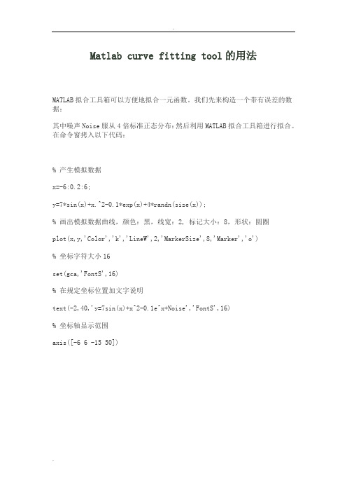
Matlab curve fitting tool的用法MATLAB拟合工具箱可以方便地拟合一元函数。
我们先来构造一个带有误差的数据:其中噪声Noise服从4倍标准正态分布:然后利用MATLAB拟合工具箱进行拟合。
在命令窗拷入以下代码:% 产生模拟数据x=-6:0.2:6;y=7*sin(x)+x.^2-0.1*exp(x)+4*randn(size(x));% 画出模拟数据曲线,颜色:黑,线宽:2, 标记大小:8,形状:圆圈plot(x,y,'Color','k','LineW',2,'MarkerSize',8,'Marker','o')% 坐标字符大小16set(gca,'FontS',16)% 在规定坐标位置加文字说明text(-2,40,'y=7sin(x)+x^2-0.1e^x+Noise','FontS',16)% 坐标轴显示范围axis([-6 6 -15 50])运行结果:Fig-1拟合步骤如下:1)打开Curve fitting tool: 在命令窗中直接键入 cftool,这时显示出拟合工具窗的GUI:Fig-22)选择Data,在X Data 和 Y Data 中选择数据,必要的话加上权数据,在 D ata set name 框中给你拟合的数据起名(例如 xy),然后按Create data set,则数据在拟合工具窗显现。
Fig-33)按Fitting 键,显示拟合编辑器:Fig-4按Creat data set,我们从数据窗中看到了刚才保存的拟合数据xy。
Fig-5在拟合曲线类型框(Type of fit)中有很多类拟合函数形式,比如选中多项式后,下面的窗口会显示不同次数的多项式选项,比如选择3次多项式(Cubic Pl oynomial)Custom Equations 代表用户自定义函数。
pdms中文教程_.结构建库

VPDVANTAGE Plant Design System工厂三维布置设计管理系统PDMS结构建库培训手册型钢库PDMS已经提供了较完善的元件库,包括型材截面、配件和节点库。
但不一定十分齐全,所以PDMS提供了非常方便的建库工具,这些功能都可在PARAGON中实现。
设计库、元件库和等级库之间的关系等级库(Specificaion)是设计库与元件库之间的桥梁。
设计者在等级库中选择元件后,等级中的元件自动找到对应的元件库中的元件;元件库中的几何形状和数据被设计库参考。
如下图。
型钢库层次结构型钢库World下包含了许多元件库和等级库,它们也是一种树状结构库。
下图就是型钢库层次结构:型钢等级库层次结构等级库相当于元件库的索引,其目的是为设计人员提供一个选择元件的界面,它的层次结构既与界面的关系如下图所示。
本章主要内容:1.定义型钢截面(Profile)2.定义型钢配件(Fitting)3.定义节点(Joint)定义型钢截面(Profile)练习一:定义型钢截面库1.元件库最终的层次结构如下:2.以管理员身份(如SYSTEM)登录PARAGON模块,再进入Paragon>Steelwork子模块。
3.在4.选择菜单Create>Section,创建新的STSE,5.在刚创建的STSE下,选择菜单Create>Element,创建三个元素:“ref.DTSE”、“ref.GMSS”和“ref.PTSS”。
现在的数据库结构如下:6.设置。
选择Settings>Referance Data… 和Display>Members…按下图设置:7.鼠标指向CATA层,选择菜单Create>Section,创建新的STSE:example/PRFL/BOX。
8.选择菜单Create>Category>For Profiles,创建新的STCA,如下图:9.鼠标指向STCA:example/PRFL/REF.DTSE层,在命令行中键入命令:“NEW DTSE /BOX/EQUAL/DTSE”,这样新建了一个DTSE,如下图。
使用Origin处理'电磁感应'实验数据教程【原创】
之后点击“Finish”,并在原来的下拉菜单中选择你新建的模型:
点击:
,即பைடு நூலகம்~
选择: 这时会自动弹出如下窗口:
输入名称(随便啦),点击“NEXT”(当然,你也可以随便改改),之后会出现下图:
注意,在这里,你应输入“自变量”、“因变量”所对应的符号。和待确定的系数。 我以一次函数拟合为例,那么填写就如下:
之后点击“Next”,之后会出现下图:
在这里↓,输入你的函数形式(模型),如"A+B*x",不要空格,符号应和你之前给出的符号 一致:
此处可以选择你要编辑的坐标轴对象:
这里的属性我就不说了,很简单:
提示一下,如果大家想把坐标刻度显示在里面,可在 处更改。
这是我完成的效果图,不算太难看吧↓
这个选项卡中的
7、其它功能 除了“多项式拟合”外,我们也可以自建函数,进行拟合,方法如下: 还是要先画散点图 之后点击“Analysis”--->“Fitting”--->“Nonlinear Curve Fit”--->“Open Dialog” 会弹出如下对话框:
“Polynomial Fit”为多项式拟合,选择其子菜单中的:“Open Dialog”--->OK 即可,当然, 你也可以更改一些相关参数。
6、美化 当然你也可以对图像进行美化,双击图表中的各元素即可完成:“颜色”、“线条粗细”等的 编辑。 下面以“坐标轴”为例,举个简单的例子:
双击坐标轴,即可弹出如下对话框:
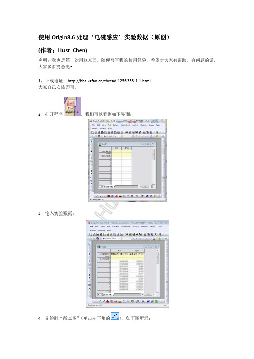
使用 Origin8.6 处理‘电磁感应’实验数据(原创) (作者:Hust_Chen)
声明:我也是第一次用这东西,随便写写我的使用经验,希望对大家有帮助。有问题的话, 大家多多提意见~
SAS公司的JMP软件培训教程

Time
8:00am 8:00am 8:00am 8:00am 8:00am 8:30am 8:30am 8:30am 8:30am 8:30am 9:00am 9:00am 9:00am 9:00am 9:00am 9:30am
File>new. 使用已有数据表单;
点击:File>open 点击如下所示的图标也可。
新建,打开,保存
8/1/2024 03:21
5
JMP操作
选择所需行或列: 连续可鼠标拖放,非连续可CTRL+CLICK
增加行及增加列: 方法1、在空白的相依行处或相应列出双
击即可增加一行或一列。 方法2、点击:Raws>Add rows增加行 点击:cols>add columns增加
在Constant前打勾,并在其后栏目内填5。
Chart Type选为Mean,R,S.并在其下的 Mean及R前的框内打勾。
选中K Sigma,并在其前的栏目内填入3。 即我们以3Sigma标准来做控制图。
8/1/2024 03:21
35
制作Xbar-R图
点击
Chart, 既可 得出 控制 图。
8/1/2024 03:2缺陷(或打开 工作表:02-jmp trma-paretochart)。
2、点击图标: Pareto Charts只将 defects加入Y。见下 页图。
3、点击OK,既可得 出柏拉图。
8/1/2024 03:21
21
柏拉图
8/1/2024 03:21
Test for Normality
如何正确的看待Fitting且正确调节坐垫高度——希望这篇推文可以帮到你!

如何正确的看待Fitting且正确调节坐垫高度——希望这篇推文可以帮到你!对于每一个资深或者即将成为资深车友的公路自行车爱好者,fitting绝对是一个绕不过去的问题,每个人都会在漫长的公路车骑行过程中碰到各种各样的疼痛、麻木、僵硬,在无数次谷歌、百度、各大论坛发帖或者看帖寻求答案无果之后,会产生一个“我一定要去作一次fitting”的想法。
一部分人作了fitting,心愿得到了满足,但我相信作过fitting的人肯定还会碰到这样或那样的问题。
这些问题到底怎样解决,如何破解fitting的迷思,下面是个人的一些看法。
一、“孩子,正确的坐垫位置是一切的开始”你也许在很多地方看到这句话,你不能对它再认同更多了,你也听说过过高或过低的坐垫位置会导致膝盖问题、肌肉不平衡、输出水平低。
基本上,很多人都陷入了坐垫位置的迷思,无法破解,只能作fitting求破解。
我的意见:一个正规的(但不一定非常贵的)fitting是应该的,fitter会用专业工具测量你的跨高,大腿和小腿的长度,测量你踩踏时膝盖弯曲的角度,最终给出你的坐垫高度(distancefrom bottom bracket to the saddle五通到坐垫距离)和setback(坐垫鼻头垂线和五通中心垂线的距离)。
这两个数据非常关键,它是你今后对公路车进行调整的基准,但是,这两个值并非一成不变,请不要以毫米为精确度让自己的新车或新坐垫符合这两个数值,理由如下:每个人都有自己骑公路车的方式,有些人从来不超过30公里每小时,有些人从来不能忍受35公里每小时以下的速度,有些人骑上车以后就像电扇一样转动他们的双腿,另外一些人则像是在爬很陡的楼梯(踏频很慢)。
不同的骑车方式对坐垫位置的影响很大,下面详细描述:A.你骑得越快,踩踏板的力度越大时,你的坐垫应该越高(坐杆拔出更多),setback值更小(坐垫往前推)。
B.你骑得越慢,或者骑得很快但是踏频也很高导致你平均踩踏力量并不高时,你的坐垫应该更加靠后,并且加大setback值。
教你如何0成本进行BikeFitting

教你如何0成本进行BikeFitting关于Bike Fitting,我们曾经转载过一篇《什么是Bike Fitting》,可是普通车友很难有机会接触到专业的Fitting,或者不愿意花大价钱去进行Fitting,有没有什么办法可以进行简单的Fitting呢?麻省理工大学的人体工程学研究实验室的一项研究发现,另一种通过肢体长度进行自行车fitting的办法可以达到98%的准确率,对于普通车友选购单车,进行简单的fitting十分具有参考价值。
Timze博士的研究中有关生物学和对称性的一些链接是很难理解的,就为大家化繁为简的讲解一下吧。
Bike Fitting有3个基本参数:座垫高度、座垫到把立距离和把立位置。
座垫到把立距离:如图,将手臂置于座垫前,中指应该刚好碰到把立的中心。
这个是用于量度座垫到把立的距离。
鞍座高度:然后确定座垫高度。
腋窝置于座垫,中指刚好碰到BB顶端。
之前的研究已经确定每人股骨和前臂的比例是永恒的,所以这个测量方式很科学。
把立的高度和长度:把立的高度和长度和座垫的位置直接关联。
由于这部分与个体灵活性大有关联,所以测量结果有些许浮动空间。
不过,研究亦已证实躯干的旋转度和手指尺寸是有必然联系的。
专业车手可用3根手指量度把立的高度(如图),把立顶端到头管顶端应是刚刚好3根手指宽度。
老人、通勤者和骑行驴友则需要4(有时甚至达5)根手指宽度。
把立长度不可调节,所以在购买时需特别留意。
如图将拇指和食指形成90°角,当拇指固定在头管顶中心时,你的中指应该和把立尾端齐平。
以上就是通过肢体进行Fitting的全部内容,是不是很简单呢?虽然并没有专业Bike Fitting那么精准,但是对于购车和简易调节已经有很高的参考价值,不需要再额外找车店甚至花钱进行Fitting了。
fitting测量方法

fitting测量方法(最新版1篇)篇1 目录1.findmotifs.pl 概述2.findmotifs.pl 的统计方法3.findmotifs.pl 的应用实例4.findmotifs.pl 的优点与局限性篇1正文1.findmotifs.pl 概述findmotifs.pl 是一种用于寻找基因调控元件的生物信息学工具,可以帮助研究者发掘基因组中的潜在调控序列。
在基因调控研究中,这些序列对于了解基因表达调控机制具有重要意义。
2.findmotifs.pl 的统计方法findmotifs.pl 主要采用统计方法来识别基因组中的潜在调控序列。
它通过对基因组数据进行深入分析,寻找其中频繁出现的短序列,从而揭示这些序列可能具有的调控功能。
具体来说,findmotifs.pl 会根据用户设定的参数,对输入的基因组数据进行筛选和排序,然后通过统计分析方法检验候选序列的显著性。
3.findmotifs.pl 的应用实例findmotifs.pl 在实际应用中可以帮助研究者快速有效地发掘基因组中的调控序列。
例如,研究者在分析某个生物体的基因组时,可以通过使用 findmotifs.pl 寻找到可能调控该生物体特定基因表达的序列。
这些序列可以为研究者提供关于基因调控机制的宝贵信息,有助于深入理解生物过程。
4.findmotifs.pl 的优点与局限性findmotifs.pl 作为一种生物信息学工具,具有以下优点:(1)高效性:findmotifs.pl 能够快速地处理大量基因组数据,为研究者节省时间和精力。
(2)准确性:通过采用统计方法,findmotifs.pl 可以在很大程度上确保所识别出的调控序列具有显著性。
然而,findmotifs.pl 也存在一定的局限性:(1)依赖输入数据质量:findmotifs.pl 的分析结果受到输入数据的影响,如果输入数据质量不高,可能会影响分析结果的准确性。
(2)需要专业技能:尽管 findmotifs.pl 操作简单,但对于生物信息学领域的研究者来说,仍需要具备一定的专业技能来正确地使用该工具并解释分析结果。
Training_AutoBlade_Fitting

初始文件准备
建立原始叶型的geomturbo文 件格式
用户界面(GUI)
进入AutoBlade_Fitting模块界面, 并,建立相应的工程项目
拓扑(结构)定义 选取目标几何文件
执行初始拟合 ห้องสมุดไป่ตู้式拟合
定义叶轮机械结构类型 (轴流?离心?)
选择将拟合的原始叶型文件 (In geomturbo file format)
1. 为什么要进行参数化拟合
在叶轮表达形式中,可以分为CAD模型、离散点模型、参数化模型,大部分的叶轮造型最 终给出的形状都是以CAD模型或者离散点形式给出的,这样描述一个三维叶轮则需要复杂的 三维曲面或者数量庞大的离散点坐标。而通过参数化拟合,可以将一个复杂的叶轮用若干个 简单的控制参数来表达,在这个基础上,使用人员可以很方面的通过控制几何参数的变化来 实现叶轮的改型。另外,对于三维叶轮的优化,如果直接对以离散点形式或者CAD模型形式 存在的叶型,则是无法实现的,因为需要控制的参数可能是成千上万个,而通过拟合后得到 参数化的叶型,在优化中,仅需要对某几个参数进行自动调整合控制,便可以得到对应的合 理叶型形状。这样,控制过程比较直观而且可靠。
3.1 3.3
3.2
Page 6
尤迈克(北京)流体工程技术有限公司
Step 3. 项目管理
1. 新建工程项目或者打开已经存在的工程文件(.iec)
2. 选择AutoBlade_Fitting功能模块
注:该提示子窗口仅会在新建工程项目 时出现,打开已有项目的操作不会出现 该选项。
Page 7
尤迈克(北京)流体工程技术有限公司
*注: 1. 初始化拟合失败,则软件会提示“Initialization process failed”的信息,此 时主要原因是: a. 几何拓扑结构的不正确造成的。此时,需要检查几何拓扑 结构; b. 对于纯离心式叶轮(例如扩压器),还需要在AutoBlade界面中的 Stacking Laws选项下,将“Meridional Location”中Additional Setting选项下的 LE和TE更改为; 2. 不正确的原始文件Geomturbo文件格式也可能导致初始化拟合失败; 3. 具体失败的原因可以从工程项目下的日志文件.log中查找。
FITTING 技术手册

610
406
1219
813
813
610
450
457.0
478
284
686
457
1372
914
914
686
500
508.0
529
316
762
508
1524
1016
1016
762
550
559
-
343
838
559
-
-
-
-
600
610
630
381
914
610
-
-
-
-
650
660
-
405
991
660
-
-
-
-
700
B16.9、ASME Bl6.11 的代号均为 AS;SHJ408、SHJ409、SHJ410 的代号均为 SH,余此类推。
7.举例说明
例 1 GBl2459 标准的公称通径 350×300、外径为 A 系列、壁厚等级 Sch40、材料为 20 的对焊异
径三通的代号为:
BTR 350×300A—S40—C2 GB 例 2 GB/T13401 标准的公称通径 600、外径为 B 系列、壁厚等级 Sch10s 材料 1Cr18Ni9Ti 的对 焊 90°长半径弯头的代号为:
Cutting Material
外观检查
Visual Examination
校形 Calibration
热处理 Heat
Treatment
成形 Forming
表面处理 Surface Treatment
平头 Cutting End
GInaFiT手册说明书
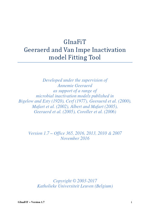
GInaFiTGeeraerd and Van Impe Inactivationmodel Fitting ToolDeveloped under the supervision ofAnnemie Geeraerdas support of a range ofmicrobial inactivation models published in Bigelow and Esty (1920), Cerf (1977), Geeraerd et al. (2000), Mafart et al. (2002), Albert and Mafart (2005),Geeraerd et al. (2005), Coroller et al. (2006) Version 1.7 – Office 365, 2016, 2013, 2010 & 2007November 2016Copyright © 2003-2017Katholieke Universiteit Leuven (Belgium)Disclaimer and SupportDisclaimerGInaFiT and this manual come without ANY WARRANTY and are provided “AS-IS”. The softwar e GInaFiT is copyrighted by the Katholieke Universiteit Leuven (KULeuven, Belgium). It is not permitted to include GInaFiT in any other application. The program is for research purposes only and should not be solely relied upon for any reason.AcknowledgementsOn publishing/presenting the results obtained with GInaFiT, you are kindly invited to refer to A.H. Geeraerd, V.P. Valdramidis, J.F. Van Impe, 2005. GInaFiT, a freeware tool to assess non-log-linear microbial survivor curves. International Journal of Food Microbiology, 102, 95-105 and to the original research publications for the model(s) you selected for your case-study (as provided in the Excel result-sheet(s) and this user manual).FeedbackIf you would have comments or suggestions regarding the installation, use or content of GInaFiT, or if you would be willing to provide a short user testimonial, please contact *****************************.be, associate professor at www.mebios.be. Your comments and user testimonials are highly appreciated.UpdatesPossible future updates will be accessible via the GInaFit homepage http://www.ginafit.be/ Compatibility with different Microsoft® Office Excel® versionsThe GInaFiT version that you have obtained together with this manual is compatible with Microsoft®Office Excel® 365, Microsoft® Office Excel® 2016, Microsoft® Office Excel® 2013, Microsoft®Office Excel® 2010 and Microsoft® Office Excel® 2007, and in principle it should work for any language (though we did obviously not test for every language). Installation instructions are provided below.Since Version 1.6 GInaFiT is not compatible anymore with Microsoft® Office Excel® 2003,also called Microsoft® Office Excel® XP. If you would be interested in receiving Version 1.5 (Version 1.7 contains bug fixes not implemented in Version 1.5) for Microsoft®Office Excel®2003/XP, please contact *****************************.be.Installation of GInaFiT Office365/2016/2013/2010For the installation instructions for GInaFiT Office 2007, please refer to page 11 of this manual.An essential requirementPlease carefully consider the following essential requirement before proceeding to the installation of GInaFiT in Office 365/2016/2013/2010: the MS-Excel Add-In “Solver” is installed.This requirement can be verified by looking under the Excel worksheet tab “Data”. Solver should be visible in the right corner, as indicated in the next figure.If the Solver is not appearing under the worksheet tab “Data”, it needs to be installed. This is to be performed by following this procedure:∙Click the File tab.∙The Microsoft Office Backstage view opens∙Click Options;∙The Options dialog box appears. Select Add-InsAt the bottom of the Add-Ins screen, select “Excel Add-Ins” und er the drop-down list next to “Manage”. It is likely (but not guaranteed) that “Excel Add-Ins” is already appearing here. Then proceed by hitting the button Go∙The item “Solver Add-in” has to be ticked in the list, i.e. the “v” should be visible before the Solver Add-In. Alternatively, it may be the case that the Solver name is indicated with its equivalent name in the language of your Windows version. If this is the case, select the Solver with this other name.∙Press OK∙The Solver should now be visible in the right corner under the Excel menu tab “Data”, as indicated in the next figure.Installation of GInaFiT.xlaIt is suggested to place the file GInaFiT.xla in the directoryc:\Program Files\Microsoft Office\Office14\ADDINSor in a similar directory for an Office version in a language different from English. Nevertheless, placing at any other location like, for example, C:\temp, is always possible.Start MS-Excel with a blank work sheet.∙Click the File tab.∙The Microsoft Office Backstage view opens∙Click Options;∙The Options dialog box appears. Select Add-Ins∙At the bottom of the Add-Ins screen, select “Excel Add-Ins” under the drop-down list next to “Manage”. It is likely (but not guaranteed) that “Excel Add-Ins” is already appearing here. Then proceed by hitting the button Go.∙In the Add-In screen tick the Add-In GInaFiT when present in the list or select the GInaFiT.xla file by browsing to the directory selected at the start of this installation procedure.∙Press OK and please read carefully the two screens appearing.∙From this moment on the button GInaFiT will be present in the Worksheet tab Add-Ins (last tab)How to remove GInaFiTStart MS-Excel with a blank work sheet.∙Click the File tab.∙The Microsoft Office Backstage view opens∙Click Options;∙The Options dialog box appears. Select Add-Ins∙At the bottom of the Add-Ins screen, select “Excel Add-Ins” under the drop-down list next to “manage”. It is likely (but not guaranteed) that “Ex cel Add-Ins” is already appearing here. Then proceed by hitting the button Go∙In the Add-In screen untick the Add-In GInaFiT.∙ A screen appears, press OK on that screen.∙Delete the GInaFiT.xla file from the directory selected at the start of the installation procedure.Installation of GInaFit Office 2007An essential requirementPlease carefully consider the following essential requirement before proceeding to the installation of GInaFiT Office 2007: the MS-Excel Add-In “Solver” is installed.This requirement can be verified by looking under the Excel worksheet tab “Data”. Solver should be visible in the right corner, as indicated in the next figure.If the Sol ver is not appearing under the worksheet tab “Data”, it needs to be installed. This is to be performed with the procedure∙Hit the Office Button (this is the Circle with the Office logo in the upper left corner of the Excel application)∙Hit the button “Excel Options”∙Select Add-Ins∙At the bottom of the Add-Ins screen, select “Excel Add-Ins” under the drop-down list next to “manage”. It is likely (but not guaranteed) that “Excel Add-Ins” is alreadyappearing here. Then proceed by hitting the button Go.∙The item “Solver Add-in” has to be ticked in the list, i.e. the “v” should be visible before the Solver Add-In. Alternatively, it may be the case that the Solver name is indicated with its equivalent name in the language of your Windows version. If this is the case, select the Solver with this other name.∙Press OK∙The Solver should now be visible in the right corner under the Excel menu tab “Data”, as indicated in the next figure.Installation of GInaFiT.xlaIt is suggested to place the file GInaFiT.xla in the directoryc:\Program Files\Microsoft Office\Office12\ADDINSor in a similar directory for an Office version in a language different from English. Nevertheless, placing at any other location like, for example, C:\temp, is always possible.Start MS-Excel with a blank work sheet.∙Hit the Office Button (this is the Circle with the Office logo in the upper left corner of the Excel application)∙Hit the button “Excel Options”∙Select Add-Ins∙At the bottom of the Add-Ins screen, select “Excel Add-Ins” under the drop-down list next to “manage”. It is likely (but not guaranteed) that “Excel Add-Ins” is already appearing here. Then proceed by hitting the button Go.∙In the Add-In screen tick the Add-In GInaFiT when present in the list or select the GInaFiT.xla file by browsing to the directory selected at the start of this installation procedure.∙Press OK and please read carefully the two screens appearing.∙From this moment on the button GInaFiT will be present in the Worksheet tab Add-Ins (last tab)How to remove GInaFiTStart MS-Excel with a blank work sheet.∙Hit the Office Button (this is the Circle with the Office logo in the upper left corner of the Excel application)∙Hit the button “Excel Options”∙Select Add-Ins∙At the bottom of the Add-Ins screen, select “Excel Add-Ins” under the drop-down list next to “manage”. It is likely (but not guaranteed) that “Excel Add-Ins” is already appearing here. Then proceed by hitting the button Go∙In the Add-In screen untick the Add-In GInaFiT.∙Delete the GInaFiT.xla file from the directory selected at the start of the installation procedure.How to use GInaFiT1.Select the data to be modelled in the Excel sheet. The first column should be time, the second columnshould be LOG10(N).2.Select the model to be applied out of the ten different models available as can be seen in the figurebelow.3. A new sheet is inserted with the same name as the name of the original sheet followed by the nameof the model selected, e.g., Sheet1 would result in Sheet1_Geeraerd_Shoulder_Tail. The result is demonstrated below.GInaFiT output when selecting the “Gee raerd et al., 2000: Log-Linear + Shoulder” Menu-Item for the case-study at hand.A short advice on the use of GInaFiTThe tool is useful for testing ten different types of microbial survival models on user-specific experimental data relating the evolution of the microbial population with time. The ten model types are: (i) classical log-linear curves, (ii) curves displaying a so-called shoulder before a log-linear decrease is apparent, (iii) curves displaying a so-called tail after a log-linear decrease, (iv) survival curves displaying both shoulder and tailing behavior, (v) concave curves, (vi) convex curves, (vii) convex/concave curves followed by tailing, (viii) biphasic inactivation kinetics, (ix) biphasic inactivation kinetics preceded by a shoulder, and (x) curves with a double concave/convex shape. The models were originally published as Bigelow and Esty (1920), Cerf (1977), Geeraerd et al. (2000), Mafart et al. (2002), Albert and Mafart (2005), Geeraerd et al. (2005) and Coroller et al. (2006).Next to the obtained parameter values, the following statistical measures are automatically reported: standard errors of the parameter values, the Sum of Squared Errors, the (Root) Mean Sum of Squared Errors, the R² and the adjusted R². In addition, t4D, the time needed for a 4 log reduction of the initial microbial population, as originally proposed by Buchanan et al. (1993), is also automatically reported (for data sets covering at least 4 decimal reductions).The tool can be used in two ways. On one hand, for end-users having already a qualitative idea of the general shape of their survival curves, the choice for one of the model types is obvious. On the other hand, if the end-user does not have a clear idea yet, two or more of the different model types available can be tested and compared. The time for a 4 decimal reduction can be useful to summarize the information present in a data set, for example, if a common survivor curve shape can not be selected for a range of different conditions tested.Additionally, the tool has some built-in features testing for mis-use, for example, when trying to identify a model with tailing on data not having a tail or when using a too limited number of data points (observations) in comparison with the number of parameters in the model type chosen (the number of parameters ranges from 2 to 5 for the ten model types available).Further illustration on the use of GInaFiT can be found in Geeraerd et al. (2005). If the use or interpretation of GInaFiT results would raise questions, please contact us at *****************************.be.ReferencesAlbert I. and P. Mafart 2005. “A modified Weibull model for bacterial inactivation”.International Journal of Food Microbiology, 100, 197-211Bigelow W.D. and J.R. Esty 1920. “The thermal death point in relation to typical thermophylic organisms”. Journal of Infectious Diseases, 27, 602Buchanan R.L., Golden M.H. and Whiting R.C. 1993. “Differentiation of the effects of pH and lactic or acetic acid concentration on the kinetics of Listeria monocytogenes inactivation”.Journal of Food Protection, 56, 474-478, 484.Cerf O. 1977. “A review. Tailing of surv ival curves of bacterial spores”. Journal of Applied Microbiology, 42, 1-19Coroller L., I. Leguerinel, E. Mettler, N. Savy and P. Mafart 2006. “General model, based on two mixed Weibull distributions of bacterial resistance, for describing various shapes of inactivation curves”. Applied and Environmental Microbiology, 72, 6493-6502.Geeraerd A.H., C.H. Herremans and J.F. Van Impe 2000. “Structural model requirements to describe microbial inactivation during a mild heat treatment”. International Journal of Food Microbiology, 59, 185-209Geeraerd A.H., V.P. Valdramidis and J.F. Van Impe 2005. “GInaFiT, a freeware tool to assess non-log-linear microbial survivor curves”. International Journal of Food Microbiology, 102, 95-105 Geeraerd A.H. and J.F. Van Impe 2007. “GinaFiT. Revealing the time-dependence of microbial survival under food processing, food preservation or environmental stress conditions”. In: Nychas, G.-J.E., Taoukis, P., Koutsoumanis, K., Van Impe, J. and Geeraerd, A. (Eds.), 5th International Conference Predictive Modelling in Foods - Conference Proceedings, 163-164, Agricultural University of Athens, Athens (ISBN 978-960-89313-7-4) [5th International Conference Predictive Modelling in Foods, Athens (Greece), 16-19 September, 2007]Mafart P., O. Couvert, S. Gaillard and I. Leguerinel 2002. “On calculating steril ity in thermal preservation methods: application of the Weibull frequency distribution model.” International Journal of Food Microbiology, 72, 107-113AcknowledgementsAnnemie Geeraerd is associate professor at the Division MeBioS –Mechatronics, Biostatistics and Sensors at the Biosystems Department at KULeuven –www.mebios.be. My colleagues Benny Depre, Maarten Hertog and Bram Van de Poel are gratefully acknowledged for their help in realizing this GInaFiT Version 1.6 and its manual. Dr. Vicente Gomez, CSIC, Spain is gratefully acknowledged for reporting a bug in Version 1.5.Mieke Janssen, Arnout Standaert, Vasilis Valdramidis and Karen Vereecken (at that time working at KULeuven/BioTeC, Department of Chemical Engineering) are gratefully acknowledged for their help in testing an earlier version of this tool, as well as Marie Cornu (who was affiliated with AFSSA, now ANSES in Paris) for her help to establish an earlier French version.Concerning the test phase of the language-independent version of GInaFiT (from Version 1.4.2 on), the following persons are especially to be acknowledged: Antonio Valero Díaz (Department of Food Science and Technology, University of Cordoba, Spain), Laurent Guillier (Ecole Nationale Vétérinaire d'Alfort, Maisons-Alfort, France), Philipp Hammer (Institute for Hygiene and Food Safety, Federal Research Center of Nutrition and Food, Kiel, Germany) and Xiaohe Wu (College of Food Science & Nutritional Engineering, China Agriculture University, Beijing, China).。
CATIA DMU Fitting 电子样车拆装分析培训教程

DMU Fitting 电子样机拆装分析
产品拆装分析可对产品拆装过程进行演示,也可在拆装过程中进行动态的 检查产品与周围零部件之间的关系。FIT包括产品拆装路径的定义和优化, 拆装过程中的动态干涉检查、工具空间校核等。
DMU拆装仿真(DMU Simulation)工具条
之后我们可以用光顺的命令对找 出的轨迹作光顺处理
轨迹记录器 (Track)
颜色变化指令 (Color Action)
编辑序列 (Edit Sequence) 编辑和进行试验 (Edit&&perform Experiment) 仿真播放器
(Player) 包络体 ( Swept Volume)
设置干涉检查模式 (Clash Detection)
距离及距离带分析 (Distance and Band Analysis)
点击出现如下对话框:
点击选择需要做出包络 体的件出现如下对话框:
路径追踪器 这个功能可以使你很容易找到最佳的拆装路径,但是在此之前你必须有一个存在 的仿真。
选择仿真后点击该命令出现:
忽略已存在的干涉。当装配的部件之间本身存在干涉,而当执行 “Path Finder”的时候不希望考虑干涉问题就把其选中。 最终结果
干涉检查(Clash)
光顺(Smooth)
爆炸视图 (Exploding)
路径追踪器
(Path finder) 复位
(Reset Position) 可拆装的组件 (Shuttle)
运动物体所留下的轨迹 点击它,会出现轨迹的对话框:
设置模拟时间
轨迹记录 轨迹修改
重新使用镜头(移动顺 序中增加另外的路径)轨迹顺序修改来自轨迹删除轨迹防真器
matlab曲线拟合

Smooth选项卡各选项的功能:
.Original data set 用于挑选需要拟合的 数据集; .Smoothed data set平滑数据的名称; .Method用于选择平滑数据的方法,每一个 相应数据用通过特殊的曲线平滑方法所计 算的结果来取代。平滑数据的方法包括: (ⅰ)Moving average 用移动平均值进 行替换; (ⅱ)Lowess局部加权散点图平滑数据, 采用线性最小二乘法和一阶多项式拟合得 到的数据进行替换;
.Smoothed data sets 对于所有平滑数 据集进行列表。可以增加平滑数据集,通 过单击Create smoothed data set按 钮,可以创建经过平滑的数据集。 .View按钮 打开查看数据集的GUI,以散点 图方式和工作表方式查看数据,可以选择 排除异常值的方法。 .Rename用于重命名。 .Delete可删去数据组。 .Save to workspace保存数据集。
.y=polyval(p,x,[],mu)
用x=(x-u1)/u2代替x,其中mu是一个
二维向量[u1,u2], u1=mean(x),u2=std(x),通过这 样处理数据,使数据合理化。
[y,delta]=polyval(p,x,s) [y,delta]=polyval(p,x,s,mu) 产生置信区间y±delta。如果误差结果服从 标准正态分布,则实测数据落在y±delta区 间内的概率至少为50%。
例:根据表中数据进行4阶多项式拟合
X 1 3 4 4 5 2 6 1 7 1 8 2 9 3 10 4 F(x) 10 5
>> >> >> >> >>
小调整让骑行更舒适:如何在家做简易fitting?骑行装备与器材公路车山地车

小调整让骑行更舒适:如何在家做简易fitting?骑行装备与器材公路车山地车这篇文章只给大家讲两个参数:Stack和Reach从水平上管设计的车架开始,上管长度一直被当做提供自行车尺寸估算值的合理指标,之所以说是估算值,因为即使同样的上管长度,不同的座管角度、不同的五通下沉量会导致Reach值(五通中心到头管中心的水平距离)不一样。
但一些品牌开始追求人性化设计的车架开始将上管设计成倾斜,意味着有更低的跨高(下车时更不容易卡住蛋),这时再依据上管长度来估算车架尺寸就会出现比较大的偏差。
倾斜上管设计的车架形式,使得根据车架上管长度来选车架的方法会跟Fitting出现较大的差异,而现代的Fitting大多以Reach值和Stack值作为选车架或搭配把组长度的依据,从下图可以看出车架设计具体的参数定义。
Reach和Stack的定义都跟五通中心和头管中心相关,不同的是Reach值是水平距离,Stack值是垂直距离;倾斜上管的车架一般不会关心上管长度,而是用有效上管长度来代替。
▲现在大多数厂商都会给出Stack和Reach参数,方便车手根据Fitting的结果来选车架一个帮我做Fitting的前同事说了一番中肯的评论:“我不管你骑的是纸箱还是什么,只要上面有五通中心和车把,我们都可以把它进行尺寸化”。
这里他并没有把量测上管或座管作为将车架尺寸化的重要参数。
过去的钢架公路车受限于设计理念和制作工艺,立管和上管的长度尺寸往往呈等比例正相关,而立管长度一般会被当作车架尺寸的参数。
随着制作工艺的改变,如今的车架设计不再墨守成规,上管长度跟立管长度比例一般都不相同,所以也就不能在用上管长度来估算车架的尺寸。
所有的这一切很大程度上是意大利设计方法和几个传统的坐垫高度量测方法来影响了车架尺寸的认定。
随着现代车架设计,在倾斜上管型式的车架上量测上管长度显然已经没有太多意义,你要是向现代的车架厂商说要订制车架,他们首先会问你的是“你需要多大的Reach和Stack值?”虽然现在也还有一些品牌坚守水平上管设计(我听到有人讲BMC,其实也不算),但是他们也不会把上管长度列入几何表,更别说现在的座管已经不是圆形的,而是水滴形或其他异型,要抓取座管中心到头管中心来量测上管长度已经很不准确了。
TutorialLigandFittingwithCoot-CCP4:教程配体配合黑鸭-CCP4

Tutorial:Ligand Fitting with CootCCP4School APS2010May20,20101IntroductionWe have a protein structure(which is well-refined).However,we have not yet identified the ligand position-indeed we don’t even know if the ligand is bound or not.In this tutorial,we will build a ligand and search the density for this ligand, add the ligand to main protein molecule and refine and validate the ligand.2Experimental DetailsThis protein is the catalytic domain of poly(ADP-ribose)polymerase2crystallised from PEG3350(polyethylene glycol),Tris and cryoprotected using glycerol.3StartingSo let’s load the protein coordinates ligand-fitting-no-ligand.pdb and the associated MTZfile which is e File→AutoOpen MTZ.4SMILESNow what is the ligand that we want tofind?It’s3-aminobenzamideFigure1:3-amino-benzamideHow do we make a3D model of this ligand?We use a SMILES string(and LIBCHECK).So what is the SMILES string for3-aminobenzamide?1available,as usual,from /coot/tutorial/If you can’t draw out the SMILES string,try this link in your browser:/cgi-bin/propertiesdraw the molecule there and hit the“Calculate Properties”button-the next pages gives you the SMILES string.We need to convert this SMILES string representation to a molecule.In Coot we do that using File→SMILES...2Enter you SMILES string in the second of the two entry boxes.Press”Go”.After a few moments(in which Coot runs LIBCHECK)a molecule will appear at the centre of the screen.Is it the molecule that you wanted?Note:check the hydrogens and planarity.5Fitting LigandsWe how the correct ligand now,So let’s move on to search the map for entities of this kind.Calculate→Other Modelling T ool→Find Ligands...We have2maps from which to choose.For now,let’s choose the2mFo-DFc map andfind density clusters above1.0sigma.Make sure that you select the correct map and protein molecule and have selected the ligand that you made with the SMILES string.Press”Find’Em!”What do you see!?Y ou should see4hits.Let’s use the Fitted Ligands dialog to navigate to these hits.Do we like all the hits?If not,why not?Let’s worry about any problematicfittings later on and for now,let’s concentrate on the nicelyfitting solutions.If you like the any of the hits,merge them into the main protein molecule.Using Calculate→Merge Molecules,In the top pane,select the ligand hits thatfit nicely by ticking them.In the lower option menu,select the protein model.Then click”Merge”.Now we have 2representations of the ligands,which can be confusing,so let’s use the Display Manager to undisplay the Fitted Ligands that we merged into the main protein.Using the Fitted Ligand dialog,navigate to the newly added monomers and optimise thefit to density-we’ll use Real Space Refinement to do e the blue target on right-hand toolbar and click an atom in the residue twice.Do you like the result of the refinement?What is the torsion angle of the carboxy-amine? 6PresentationWe can emphasise the atom positions using Extensions→Representations→Hi-light Interesting Site.Nice?Maybe...2Note that thefirst line is the three letter code,conventionally this is3uppercase letters,e.g.LIG, DRG,XXX.Note that if you use several different SMILES strings,they each should have a different 3-letter-code.7Problem AreasOK,now we havefitted the nicelyfitting ligands,let’s go back to the problematic blobs.Validate→Find unmodelled blobsWe shall search the2mFo-DFc as did previously using the same protein model (which now has the3-aminobenzamidefitted).Press”Find blobs”3 We should get a dialog with two blobs listed.Examine those two blobs.We know that3-aminobenzamide does notfit these blobs well.What else could these blobs be?Let’s look at the crystallization and freezing conditions?Any clues?Now,we don’t necessarily know the3-letter-codes of the molecules that might fit these blobs.We can use the searching tool in Coot to convert between a molecule name and its3-letter-code.File→Search Monomer Library...add the molecule name to the entry box and press”Search”You will see a list of molecule that include the text you typed as part of the molecule names.If you click on any of those buttons,Coot runs LIBCHECK and generates a molecule and puts it at the centre of the screen.You can do this for the3or4different molecules that you think this blob might be.The centre of the screen is a bit crowded now.Undisplay those new ligands.To easily identify the bestfitting ligand at the site,let’s do ligandfitting here.Calculate→Other Modelling T ools→Find LigandsSelect the2mFo-DFc map as usual,and the main protein as before and the ligands to search for are the3or4newly created ligands.This time we will Search”Right Here”.You can turn onflexible ligands if you like,but this will slow down the search considerably.8Tidying UpReal Space refinement is the tool to tidy things ing the blue circle icon on the right,then click click on an atom in the residue4.When we are happy with ourfit,we can merge this new ligand into the main protein ligand as we did before.9NCS LigandsYou may have noticed by now that there are2protein chains related by non-crystallographic symmetry.We can exploit this NCS to helpfit ligands.We have fitting a ligand that bound to the”A”chain,now let’s use NCS to position a ligand in related position in the”B”chain of the protein.Extensions→NCS→NCS Ligands...The protein with the NCS is the main protein as usual,the molecule containing the ligand is also the main protein as usual(if we have done the merge mentioned above).We need to know the chain ID of the ligand that we havefitted into the ”A”chain,to do that double left-click an an atom in the ligand.In the graphics you will see something like:"C1/1XXX/E"-so the chain-id is"E".Also the status bar at the bottom shows information about the clicked atom.3we could also use Validate→Difference Map Peaks to navigate to these positions.4or(quicker)simply press the”R”key(if you have the key bindings set up).So enter that chain-id in the”Molecule containing ligand””Chain ID”entry. Then”Find Candidate positions”.Afitted ligands dialog box pops up and you can use the buttons in that dialog to navigate to the NCS ligand positions.Refine this NCS ligand position if needed and merge it into the main molecule. 10For the AdventurousIf you are feeling adventurous,you can run refmac:Calculate→Model/Fit/Refine →Run Refmac...Choose an MTZfile for Refmac and use thefile selector to choose the same MTZfile that we used in the beginning.Examine the resulting molecule.Are there any problems left tofix?。
PDMS教程 3
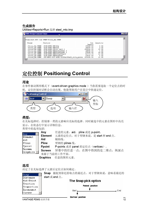
生成报告Utilities>Reports>Run 选择 steel_mto.tmp定位控制 Positioning Control用途在事件驱动图形模式下(event-driven graphics mode )当你需要选取一个定位点的时候,定位控制对话框会自动出现。
他能帮助用户在设计中快速定位。
类型:在光标选择时,控制那一类的元素响应光标的选择。
同时被选中的元素在图形中高亮显示,在状态行中显示详细信息。
类型中的选项包括:Any 任意的元素,aid , pline 或是 p-point 。
Element 元素的定位点,对于型钢来说,是start 和end 点。
Aid 辅助线。
Pline 型钢的 plines 线。
Ppoint P-points 或者 panel 的定位点(vertices )。
Screen 屏幕中的任意一点,在图中得到的是二维点,纵深点来源于当前的工作平面。
Graphics 任意的图形元素。
选项决定了在光标选择了元素后定位点如何确定。
Snap 捕捉到靠近拾取点的最近点。
对于型钢来说,意味着最近的Distance在输入栏中输入数值,光标能拾取到距最近捕捉点给定距离的点。
负值则向相反方向。
Mid-Point光标拾取到中心点。
Fraction 在输入栏中输入分割份数,光标捕捉到最近的分割点。
Proportion 在输入栏中输入分割比例,光标捕捉到最近的分割点。
例如0.25 。
Intersect两个元素的交点。
Cursor光标在元素上拾取的任意一点。
练习十七:组LIST1.点取Creat Lists按钮,弹出List/Collections对话框。
2.A dd->List,键入描述为A。
3.在Member List中定位到设备框架柱子SBFR EQUIPRACK/MAIN/COLUMNS。
4.Add->CE members,完成后关闭对话框。
练习十八:修改型钢截面形式将设备框架柱子截面形式改成混凝土形式。
fitting测量方法

fitting测量方法(原创实用版)目录1.FITTING 测量方法的概述2.FITTING 测量方法的步骤3.FITTING 测量方法的优缺点4.FITTING 测量方法的应用案例正文一、FITTING 测量方法的概述FITTING 测量方法是一种用于测量物体大小、形状和表面特性的科学方法。
它通过将测量数据与数学模型相结合,从而得到物体的精确信息。
FITTING 测量方法广泛应用于各种领域,如机械制造、航空航天、生物医学等。
二、FITTING 测量方法的步骤FITTING 测量方法主要包括以下几个步骤:1.采集数据:首先需要对物体进行测量,获取其大小、形状等各方面的数据。
2.选择模型:根据测量数据和物体的特性,选择合适的数学模型来描述物体。
3.拟合参数:将测量数据代入数学模型,通过最小二乘法或其他优化算法,求解模型中的参数。
4.验证模型:通过比较拟合后的模型与实际测量数据的误差,判断模型的准确性和可靠性。
5.应用模型:将拟合得到的模型应用于实际问题中,如预测物体在不同条件下的性能等。
三、FITTING 测量方法的优缺点FITTING 测量方法具有以下优点:1.高精度:通过拟合参数,可以得到物体的精确信息。
2.适用范围广:几乎适用于所有需要测量物体大小、形状和表面特性的领域。
3.灵活性:可以根据实际需求选择不同的数学模型,具有较强的适应性。
然而,FITTING 测量方法也存在一定的缺点:1.对初始参数敏感:在拟合过程中,初始参数的设置会对拟合结果产生较大影响。
2.计算复杂度高:拟合过程涉及到高维空间的搜索,计算量较大。
3.受测量数据质量影响:测量数据的质量对拟合结果具有直接影响。
四、FITTING 测量方法的应用案例FITTING 测量方法在许多领域都有广泛应用,例如:1.在航空航天领域,FITTING 方法可以用于测量飞行器的外形,以确保其在特定条件下的飞行性能。
2.在生物医学领域,FITTING 方法可以用于测量人体器官的尺寸,为疾病诊断和治疗提供依据。
fitting测量方法

fitting测量方法拟合是一种常用的测量方法,它可以帮助确定一个函数或数学模型与实际数据的拟合程度。
拟合方法在科学研究中广泛应用于数据处理、模型选择和参数估计等领域。
本文将介绍拟合的基本概念、常见的拟合方法以及实际应用中的注意事项。
拟合的基本概念:拟合是指通过调整函数或模型的参数,使其与实际测量数据最为吻合。
在拟合过程中,拟合函数与实际数据之间的离差最小化是一种常见的目标。
拟合分为线性拟合和非线性拟合两种类型。
线性拟合是指通过调整线性函数的斜率和截距,使其与数据点之间的离差最小化。
非线性拟合是指通过调整一般的非线性函数,使其与数据点之间的离差最小化。
常见的拟合方法:1.最小二乘法:最小二乘法是一种常见的拟合方法,它通过最小化拟合函数与实际数据之间的平方差,来确定最佳拟合参数。
最小二乘法广泛应用于线性和非线性拟合中。
在线性拟合中,最小二乘法可以通过矩阵求解来得到解析解。
在非线性拟合中,最小二乘法常用于迭代求解,通过反复调整参数值来逼近最佳拟合结果。
2.曲线拟合:曲线拟合用于拟合非线性函数或曲线。
曲线拟合可以通过最小二乘法和其他优化算法来实现。
常见的曲线拟合方法包括多项式拟合、指数拟合和幂函数拟合等。
在实际应用中,选择合适的曲线形式可以帮助准确拟合数据。
3.非参数拟合:非参数拟合是指基于统计方法,不对拟合函数做任何假设,直接通过测量数据得到拟合结果。
常见的非参数拟合方法包括核密度估计、最小距离估计和局部回归估计等。
非参数拟合在复杂数据分析中具有灵活性和鲁棒性的优势。
拟合的注意事项:1.数据预处理:在进行拟合之前,需要对原始数据进行预处理。
常见的数据预处理包括异常值处理、缺失值处理和数据平滑等。
预处理可以提高拟合结果的准确性和稳定性。
2.模型选择:拟合过程中需要选择合适的拟合模型。
选择模型需要考虑数据的特点和研究目标。
一般来说,简单模型比复杂模型更容易解释和应用,但可能对数据的拟合效果较差。
模型选择可以通过信息准则、交叉验证和贝叶斯估计等方法来进行。
- 1、下载文档前请自行甄别文档内容的完整性,平台不提供额外的编辑、内容补充、找答案等附加服务。
- 2、"仅部分预览"的文档,不可在线预览部分如存在完整性等问题,可反馈申请退款(可完整预览的文档不适用该条件!)。
- 3、如文档侵犯您的权益,请联系客服反馈,我们会尽快为您处理(人工客服工作时间:9:00-18:30)。
Copyright DASSAULT SYSTEMES 2002
7
About Shuttle
Create a group of objects to be manipulated in a Track action
Manipulator
Shuttles are groups of components placed everywhere in the assembly.
2
Copyright DASSAULT SYSTEMES 2002
Table of Contents
PRODUCT SYNTHESIS SOLUTIONS: DMU Fitting Table of Contents Fitting Customization Customizing Fitting Managing Actions About Tracks Actions About Shuttles Defining Time Duration of each Track Segment Editing Track Object ject General Process: Creating a Track Exporting / Importing Tracks Managing Fitting Simulations Managing Sequences Editing Gantt Chart Checking Clash Generating Video Files Performing an Experiment Browsing an Experiment Using Specific Tools Finding Path Automatically Smoothing Path Computing Swept Volume Exploding Course Summary
Copyright DASSAULT SYSTEMES 2002
1-2 3 4 5 6 7 8 9 10 11 12 13 14 15 16 17 18 19 20 21 22 23 24 25
3
Fitting Customization
You will become familiar with Fitting options
The Smart Target feather can be used for moving shuttle Smart Target allows you to move components with accurately 1) 2) 3) 4) 5) Double-click on the shuttle you want to move in the specification tree click Double-click on the Target Icon inside the Manipulation dialog box click Select the component you want to move and next a geometry of it (point, lane, axis etc.) Select on the second component (where you want the first one to be moved) another geometry (point, lane, axis etc.) Select a geometric element on the shuttle and then on the on the receiving component
Create a multi-speed Track to simulate real mounting/demounting process speed
When you are creating your Track you can set a different speed for each part of it: - Click on the More button - You can see a blue time bar - The green lines correspond to the intermediates shots - Drag-and-Drop these lines to modify the duration of each segment Drop
Customizing Fitting
Copyright DASSAULT SYSTEMES 2002
4
Customizing Fitting
You will define thanks to the Customization:
-The default Options for Shuttles Angular Validation -The automatic smooth -The activation of Clash beep -The automatic Track update -The default options for Automatic Insert - The deactivation of static clash -The Default Manipulation mode during simulation -Define Snap sensitivity -Use Voxelisation for Fast Clash detection
- It is less useful in Spline mode because it modifies the tack to keep spline continuity - That does not affect the total track time
Copyright DASSAULT SYSTEMES 2002 10
In this course you will learn the V5R8 DMU Fitting Specific Tools
Targeted audience
Designers
Prerequisites:
0.5 day
DMU Basic V5R9 DMU Navigator V5R9 DMU Space Analysis V5R9
Copyright DASSAULT SYSTEMES 2002 6
About Track Action
A Track is a single path easily accessible in order to mount and un un-mount products It is the same work that in DMU Navigator : In Navigator you use Tracks essentially for Cameras In Fitting you use Tracks for Products and Shuttles
When the moving object is a Camera or a Section plane: clicking the Edit button display the Properties dialog box.
Copyright DASSAULT SYSTEMES 2002
11
General Process: Creating a Track
1
From CATIA Window Select the product and choose the interpolo define time duration of each segment
4
Record the new position in the track when satisfied Modify the product position
A shuttle is defined by: Shuttle Axis Components (shuttles, parts, product…) Optionally: a reference and/ or Angle limitation
Shuttle axis
Use this option to move one shuttle relatively to another shuttle or product
CATIA Training
Foils
DMU Fitting Simulator
Version 5 Release 9 June 2002 EDU-DMU-E-FIT-FF-V5R9 EDU
Copyright DASSAULT SYSTEMES 2002
1
DMU Fitting
Objectives of the Course
In the case of the Shuttle as reference, the reference shuttle is displayed as children.
Vector
Angle
Copyright DASSAULT SYSTEMES 2002
8
Moving components within a Shuttle
(5)
(3)
Copyright DASSAULT SYSTEMES 2002
(4)
A coincidence constraint is created
Another coincidence constraint is created
9
Defining Time Duration of each Track Segment
Copyright DASSAULT SYSTEMES 2002
5
Managing Actions
You will become familiar with Track Manipulation