模数转换器(ADC)的几种主要类型
常用的几种类型的ADC基本原理及特点

常用的几种类型的ADC基本原理及特点ADC(Analog-to-Digital Converter)是将模拟信号转换为数字信号的电路设备。
常用的几种类型的ADC包括逐次逼近型ADC、闲置型ADC、逐次逼近逐比例型ADC和Σ-Δ ADC。
以下将对这几种ADC的基本原理及特点进行详细介绍。
1.逐次逼近型ADC:逐次逼近型ADC是一种较为常见的ADC类型,它的基本原理是通过逐步逼近的方式将输入的模拟信号转换为数字信号。
它的特点如下:-逐次逼近型ADC采用“二分法”的思路进行逼近,通过与参考电压的比较,逐渐缩小量化的范围,最终得到相应的数字编码。
-逐次逼近型ADC的精度受到量化误差的影响,即使进行足够多次的逼近,也无法完全消除量化误差。
-逐次逼近型ADC可以通过增加逼近的次数来提高精度,但这也会增加转换的时间。
-逐次逼近型ADC适用于中等精度要求的应用场景,如音频信号的采集与处理。
2.闲置型ADC:闲置型ADC是一种高效率、低功耗的ADC类型,其基本原理是通过比较参考电压和输入信号的大小来进行转换。
它的特点如下:-闲置型ADC通过比较器和逻辑电路进行信号转换,具有较快的转换速度和较低的功耗。
-闲置型ADC的精度受到比较器的精度限制,比较器的噪声和非线性等因素会对转换精度产生影响。
-闲置型ADC适用于要求高速转换和低功耗的应用场景,如无线通信系统和嵌入式系统。
3.逐次逼近逐比例型ADC:逐次逼近逐比例型ADC是一种综合了逐次逼近和闲置两种ADC的优点的混合型ADC,其基本原理是通过逼近和比例两个步骤完成信号的转换。
它的特点如下:-逐次逼近逐比例型ADC先进行逐步逼近的过程,然后在逼近的基础上通过比例运算进行转换,可以提高转换的精度。
-逐次逼近逐比例型ADC的特点与逐次逼近型ADC和闲置型ADC相结合,既具有逐次逼近型ADC的高精度,又具有闲置型ADC的高效率和低功耗。
-逐次逼近逐比例型ADC适用于对高分辨率和高速转换要求的应用,如高性能音频处理和图像采集。
ADC选型经典指南
ADC选型手册一ADC的定义模数转换器即A/D转换器,或简称ADC,(简称a/d转换器或adc,analog to digital converter)通常是指一个将模拟信号转变为数字信号的电子元件。
通常的模数转换器是将一个输入电压信号转换为一个输出的数字信号。
由于数字信号本身不具有实际意义,仅仅表示一个相对大小。
故任何一个模数转换器都需要一个参考模拟量作为转换的标准,比较常见的参考标准为最大的可转换信号大小。
而输出的数字量则表示输入信号相对于参考信号的大小。
二 ADC的基本原理在A/D转换中,因为输入的模拟信号在时间上是连续的,而输出的数字信号是离散量,所以进行转换时只能按一定的时间间隔对输入的模拟信号进行采样,然后再把采样值转换为输出的数字量。
通常A/D转换需要经过采样、保持量化、编码四个步骤。
也可将采样、保持合为一步,量化、编码合为一步,共两大步来完成。
(1)采样和保持:采样,就是对连续变化的模拟信号进行定时测量,抽取其样值。
采样结束后,再将此取样信号保持一段时间,使A/D转换器有充分的时间进行A/D转换。
采样-保持电路就是完成该任务的。
其中,采样脉冲的频率越高,采样越密,采样值就越多,其采样-保持电路的输出信号就越接近于输入信号的波形。
因此,对采样频率就有一定的要求,必须满足采样定理即:fs≥2fImax其中fImax 是输入模拟信号频谱中的最高频率(2)量化和编码:所谓量化,就是把采样电压转换为以某个最小单位电压△ 的整数倍的过程。
分成的等级称为量化级 ,A 称为量化单位。
所谓编码 , 就是用二进制代码来表示量化后的量化电平。
采样后得到的采样值不可能刚好是某个量化基准值 , 总会有一定的误差 , 这个误差称为量化误差。
显然 , 量化级越细 , 量化误差就越小 , 但是 , 所用的二进制代码的位数就越多 , 电路也将越复杂。
量化方法除了上面所述方法外 , 还有舍尾取整法 , 这里不再赘述。
AD和DA转换器的分类及其主要技术指标

AD和DA转换器的分类及其主要技术指标AD和DA转换器(Analog-to-Digital and Digital-to-Analog converters)是电子设备中常用的模数转换器和数模转换器。
AD转换器将连续的模拟信号转换成对应的离散数字信号,而DA转换器则将离散的数字信号转换成相应的连续模拟信号。
本篇文章将介绍AD和DA转换器的分类以及它们的主要技术指标。
一、AD转换器分类AD转换器主要分为以下几个类型:1.逐次逼近型AD转换器(Successive Approximation ADC)逐次逼近型AD转换器是一种常见且常用的AD转换器。
它采用逐渐逼近的方法逐位进行转换。
其基本原理是将模拟输入信号与一个参考电压进行比较,不断调整比较电压的大小,确保比较结果与模拟输入信号的差别小于一个允许误差。
逐次逼近型AD转换器的转换速度相对较快,精度较高。
2.模数积分型AD转换器(Sigma-Delta ADC)模数积分型AD转换器是一种利用高速和低精度的ADC与一个可编程数字滤波器相结合的技术。
它通过对输入信号进行高速取样并进行每个采样周期的累积和平均,降低了后续操作所需的带宽。
模数积分型AD转换器具有较高的分辨率和较好的线性度,适用于高精度应用。
3.并行型AD转换器(Parallel ADC)并行型AD转换器是一种通过多个比较器并行操作的AD转换器。
它的转换速度较快,但其实现成本相对较高。
并行型AD转换器适用于高速数据采集和信号处理。
4.逐渐逼近型AD转换器(Ramp ADC)逐渐逼近型AD转换器是一种通过线性递增电压与输入信号进行比较的转换器。
它利用逐渐逼近的方法寻找与输入信号最接近的电压值,然后以此电压值对应的时间来估计输入信号的值。
逐渐逼近型AD转换器转换速度较慢,但精度较高。
5.其他类型AD转换器除了上述几种常见的AD转换器类型外,还有其他一些特殊的AD转换器类型,如比例调制型AD转换器、索耳转换器等。
模数转换器(ADC)原理及分类
模数转换器(ADC)原理及分类解析在仪器仪表系统中,常常需要将检测到的连续变化的模拟量如:温度、压力、流量、速度、光强等转变成离散的数字量,才能输入到计算机中进行处理。
这些模拟量经过传感器转变成电信号(一般为电压信号),经过放大器放大后,就需要经过一定的处理变成数字量。
实现模拟量到数字量转变的设备通常称为模数转换器(ADC),简称A/D。
通常情况下,A/D转换一般要经过取样、保持、量化及编码4个过程。
取样是将随时间连续变化的模拟量转换为时间离散的模拟量。
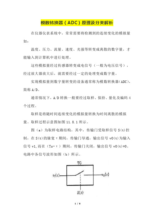
取样过程示意图如图11.8.1所示。
图(a)为取样电路结构,其中,传输门受取样信号S(t)控制,在S(t)的脉宽τ期间,传输门导通,输出信号vO(t)为输入信号v1,而在(Ts-τ)期间,传输门关闭,输出信号vO(t)=0。
电路中各信号波形如图(b)所示。
图11.8.1 取样电路结构(a)图11.8.1 取样电路中的信号波形(b)通过分析可以看到,取样信号S(t)的频率愈高,所取得信号经低通滤波器后愈能真实地复现输入信号。
但带来的问题是数据量增大,为保证有合适的取样频率,它必须满足取样定理。
取样定理:设取样信号S(t)的频率为fs,输入模拟信号v1(t)的最高频率分量的频率为fimax,则fs与fimax必须满足下面的关系fs ≥2fimax,工程上一般取fs>(3~5)fimax。
将取样电路每次取得的模拟信号转换为数字信号都需要一定时间,为了给后续的量化编码过程提供一个稳定值,每次取得的模拟信号必须通过保持电路保持一段时间。
取样与保持过程往往是通过取样-保持电路同时完成的。
取样-保持电路的原理图及输出波形如图11.8.2所示。
图11.8.2 取样-保持电路原理图图11.8.2 取样-保持电路波形图电路由输入放大器A1、输出放大器A2、保持电容CH和开关驱动电路组成。
电路中要求A1具有很高的输入阻抗,以减少对输入信号源的影响。
为使保持阶段CH上所存电荷不易泄放,A2也应具有较高输入阻抗,A2还应具有低的输出阻抗,这样可以提高电路的带负载能力。
adc模数转换器原理

adc模数转换器原理模数转换器(ADC)是一种非常重要的电子电路,它可以将模拟信号转换为数字信号,以便电路中的微处理器可以对其进行处理。
随着科技的发展,ADC的性能也在不断提高,可以提供更多功能和性能,以满足不断变化的需求。
本文将重点介绍ADC的工作原理,以及其在现有技术中的应用。
ADC的基本原理是将模拟信号(如模拟电压或电流)转换成数字信号,然后通过串行数据总线将其传送到微处理器其他部分。
ADC的类型主要分为抽样-持续转换(SAR)和按位逐次抽样(S&S)两种,其中SAR类型ADC更加常用。
SAR类型ADC的工作原理主要是将电路中的输入信号反复地采样,并使用内部电压参考或外部电压参考进行比较,以确定最终输出值。
采样率和参考电压是控制转换精度的关键因素,采样率越高,参考电压越精准,最终转换的精度就越高。
此外,随着科技的发展,ADC的性能也在不断提高。
近年来,ADC 技术可以实现多种性能,如低功耗、高动态范围、高采样率和高精度等功能。
通过不断的技术进步,ADC已经可以用于传感器、医疗影像、音频应用、声纳应用、无线通信和军事应用等多个领域。
最后,ADC技术也取得了很大的发展,能够为上述应用提供更优质的服务。
例如,最新的ADC技术可以实现低功耗、高转换速率和极高的精度,以满足当今快速变化的应用需求。
综上所述,ADC模数转换器是一种关键电路,它可以将模拟信号转换为数字信号,以便电路中的微处理器可以对其进行处理。
它的原理是采样-持续转换,依靠内部或外部参考电压进行比较,以确定最终输出值,并可用于多种应用场合,比如传感器、音频应用等。
由于技术的不断进步,ADC可以实现低功耗、高转换速率和极高的精度,以满足现有应用的需求。
ADC的结构方案概述
ADC的结构方案概述ADC,即模数转换器(Analog-to-Digital Converter),是将模拟信号转换为数字信号的一种电子设备。
在现代电子技术中,ADC广泛应用于各个领域,如通信、控制系统、医疗设备等。
ADC的结构设计有多种方案,本文将对其中的几种典型结构进行概述和介绍。
1.逐次逼近型ADC逐次逼近型ADC是最常见的一种结构方案。
它采用一个逐次逼近算法,从最高位开始逐步逼近输入信号的大小。
该结构主要包括一个比较器、一个数字-模拟转换器和一个数字逻辑控制器。
在每个时钟周期内,逻辑控制器生成一个比较阈值,并将其与输入信号进行比较。
根据比较结果,控制器调整阈值,逐步逼近输入信号的大小,直至达到所需精度。
逐次逼近型ADC的优点是结构简单、实现容易。
缺点是转换速度较慢,适用于低速应用场景。
2.并行型ADC并行型ADC是一种高速的转换器结构方案。
它使用多个比较器并行工作,将输入信号划分成多个子区间,然后分别进行转换。
每个子区间由一个比较器和一个数字-模拟转换器处理。
最后,将各个子区间的数字结果合并,得到最终的转换结果。
并行型ADC的优点是高速、高精度,适用于需要高速转换的应用。
缺点是硬件成本高,布线复杂。
3. Sigma-Delta型ADCSigma-Delta型ADC是一种低速高精度的转换器方案,常用于声音和音频信号的数字化处理。
它利用了噪声和过采样的技术,将输入信号与一个高频的参考信号进行混合,并通过一个积分运算器对混合信号进行积分平均。
通过高频参考信号的累积效应,有效抑制了噪声对转换结果的影响。
最后,通过一个数字滤波器对输出进行滤波,得到最终的数字结果。
Sigma-Delta型ADC的优点是高精度、抗干扰能力强。
缺点是转换速度较慢,不适用于高速应用。
4.均匀量化型ADC均匀量化型ADC是一种基于均匀量化原理的转换器方案。
它采用一个多电平比较器和一个分级量化器进行转换。
多电平比较器将输入信号与一组参考电平进行比较,然后将比较结果转化为数字码。
ADC的分类比较及性能指标
ADC的分类比较及性能指标1 A/D转换器的分类与比较 (1)1.1 逐次比较式ADC (1)1.2 快闪式(Flash)ADC (2)1.3 折叠插值式(Folding&Interpolation)ADC (3)1.4 流水线式ADC (4)1.5 ∑-Δ型ADC (6)1.6 不同ADC结构性能比较 (6)2 ADC的性能指标 (7)2.1 静态特性指标 (7)2.2 动态特性指标 (11)1 A/D转换器的分类与比较A/D转换器(ADC)是模拟系统与数字系统接口的关键部件,长期以来一直被广泛应用于雷达、通信、电子对抗、声纳、卫星、导弹、测控系统、地震、医疗、仪器仪表、图像和音频等领域。
随着计算机和通信产业的迅猛发展,进一步推动了ADC在便携式设备上的应用并使其有了长足进步,ADC正逐步向高速、高精度和低功耗的方向发展。
通常,A/D转换器具有三个基本功能:采样、量化和编码。
如何实现这三个功能,决定了A/D转换器的电路结构和工作性能。
A/D转换器的分类很多,按采样频率可划分为奈奎斯特采样ADC和过采样ADC,奈奎斯特采样ADC又可划分为高速ADC、中速ADC和低速ADC;按性能划分为高速ADC和高精度ADC;按结构划分为串行ADC、并行ADC和串并行ADC。
在频率范围内还可以按电路结构细分为更多种类。
中低速ADC可分为积分型ADC、过采样Sigma-Delta型ADC、逐次逼近型ADC、Algonithmic ADC;高速ADC可以分为闪电式ADC、两步型ADC、流水线ADC、内插性ADC、折叠型ADC和时间交织型ADC。
下面主要介绍几种常用的、应用最广泛的ADC结构,它们是:逐次比较式(S A R)ADC、快闪式(F l a s h)ADC、折叠插入式(F o ld i n g&Interpolation)ADC、流水线式(Pipelined)ADC和∑-Δ型A/D转换器。
1.1 逐次比较式ADC图1 SAR ADC原理图图1是SAR ADC的原理框图。
adc的种类工作原理和用途

adc的种类工作原理和用途ADC(Analog-to-Digital Converter)即模数转换器,是一种电子设备,用于将连续的模拟信号转换成离散的数字信号。
ADC在现代电子设备中得到了广泛的应用,下面将详细介绍ADC的种类、工作原理和用途。
一、ADC的种类根据其工作原理和结构,ADC可以分为以下几种主要类型:1. 逐次逼近式(Successive Approximation)ADC:逐次逼近式ADC 采用逼近法对输入模拟信号进行逐级逼近,最终得到一个数字输出。
它通过与模拟输入进行比较,并根据比较结果逐步逼近输入信号的真实值。
逐次逼近式ADC是一种广泛应用的ADC类型,具有较高的转换速度和较低的功耗。
2. 并行式ADC(Parallel ADC):并行式ADC将模拟信号按位数进行分割,每个位数均通过特定的电路进行转换,最后将结果合并成一个完整的数字输出。
并行式ADC具有较高的转换速度,但由于其需要大量的电路,使得成本和功耗较高。
3. 逐次逼近型逐次逼近系统(Pipeline ADC):逐次逼近型逐次逼近系统采用多级的逐次逼近ADC进行串联,以提高整个系统的转换速度。
每个电路将输入信号一次逼近一位,并将逼近结果传到下一级,直到最终得到完整的数字输出。
逐次逼近型逐次逼近系统ADC具有较高的转换速度和较低的功耗,广泛应用于高速数据转换领域。
4. Sigma-Delta ADC:Sigma-Delta ADC采用了过采样和噪声整形的技术,通过对输入信号进行高速取样,然后通过滤波器和数字处理器来获取高精度的输出。
Sigma-Delta ADC具有较高的转换精度和动态范围,常用于音频和通信等领域。
二、ADC的工作原理ADC的工作原理主要是将模拟信号经过一系列的步骤转换成数字信号。
以下是一般ADC的工作流程:1.采样:将模拟信号在采样保持电路中进行取样,将连续的模拟信号转换为离散的样本。
2.量化:将采样后的模拟信号转换为相应的数字数值。
ADC分类及参数

ADC分类•直接转换模拟数字转换器〔Direct-conversion ADC〕,或称Flash模拟数字转换器〔Flash ADC〕•循续渐近式模拟数字转换器〔Successive approximation ADC〕•跃升-比较模拟数字转换器〔Ramp-pare ADC〕•威尔金森模拟数字转换器〔Wilkinson ADC•集成模拟数字转换器〔Integrating ADC〕•Delta编码模拟数字转换器〔Delta-encoded ADC〕•管道模拟数字转换器〔Pipeline ADC〕•Sigma-Delta模拟数字转换器〔Sigma-delta ADC〕•时间交织模拟数字转换器〔Time-interleaved ADC〕•带有即时FM段的模拟数字转换器•时间延伸模拟数字转换器〔Time stretch analog-to-digital converter, TS-ADC1、闪速型2、逐次逼近型3、Sigma-Delta型1. 闪速ADC闪速ADC是转换速率最快的一类ADC.闪速ADC在每个电压阶跃中使用一个比较器和一组电阻.2. 逐次逼近ADC逐次逼近转换器采用一个比较器和计数逻辑器件完成转换.转换的第一步是检验输入是否高于参考电压的一半,如果高于,将输出的最高有效位<MSB>置为1.然后输入值减去输出参考电压的一半,再检验得到的结果是否大于参考电压的1/4,依此类推直至所有的输出位均置"1"或清零.逐次逼近ADC所需的时钟周期与执行转换所需的输出位数相同.3. Sigma-delta ADCSigma-delta ADC采用1位DAC、滤波和附加采样来实现非常精确的转换,转换精度取决于参考输入和输入时钟频率.Sigma -delta转换器的主要优势在于其较高的分辨率.闪速和逐次逼近ADC采用并联电阻或串联电阻,这些方法的问题在于电阻的精确度将直接影响转换结果的精确度.尽管新式ADC采用非常精确的激光微调电阻网络,但在电阻并联中仍然不甚精确.sigma-delta转换器中不存在电阻并联,但通过若干次采样可得到收敛的结果.Sigma-delta转换器的主要劣势在于其转换速率.由于该转换器的工作机理是对输入进行附加采样,因此转换需要耗费更多的时钟周期.在给定的时钟速率条件下,Sigma-delta转换器的速率低于其它类型的转换器;或从另一角度而言,对于给定的转换速率,Sigma-delta转换器需要更高的时钟频率.Sigma-delta转换器的另一劣势在于将占空<duty cycle>信息转换为数字输出字的数字滤波器的结构很复杂,但Sigma-delta转换器因其具有在IC裸片上添加数字滤波器或DSP功能而日益得到广泛应用.Atmel AVR127: Understanding ADC ParametersThis application note is about the basic concepts of analog-to-digital converter <ADC> and the parameters that determine the performance of an ADC.These ADC parameters are of good importance since they determine the accuracy of the ADC’s output.The parameters can be broadly classified into static performance parameters and dynamic performance parameters.Static performance parameters are those parameters that are not relatedto ADC’s input signal.These parameters are measured and analyzed for all types of ADCs<ADCs integrated within the microcontroller or standalone ADCs whose operating frequency are usually higher>.Instead, dynamic performance parameters are related to ADC’s input signal and their effects are significant with higher frequencies.Major static parameters include gain error, offset error, full scale error and linearity errorswhereas some important dynamic parameters include signal-to-noise ratio <SNR>, total harmonic distortion <THD>,signal to noise and distortion <SINAD> and effective number of bits <ENOB>. Basic ConceptsAn ADC is an electronic system or a module that has analog input, reference voltage input and digital outputs.The ADC convert the analog input signal to a digital output value that represents the size of the analog input paring to the reference voltage.It basically samples the input analog voltage and produces an output digital code for each sample taken.Figure 1-1. Basic diagram of ADCTo get a better picture about the ADC concepts, let us first look into some basic ADC terms used.1.1 Input Voltage RangeThe input voltage range of an ADC is determined by the reference voltage<VREF> applied to the ADC.A reference voltage can be either internal voltage or external voltage by applying a voltage on an external pin of the microcontroller.Generally reference voltage can be selected by configuring the corresponding register’s bit field of the microcontroller.ADC will saturate with a analog voltage higher than the reference voltage,so the designer must make sure that the analog input voltage does not exceed the reference voltage.The input voltage range is also called as conversion range.If ADC runs in signed mode <the mode produces signed output codes>, it allows negative analog input voltages.In such cases the analog input range is from –VREF to +VREF.An ADC which accepts both positive and negative input voltages is calledas bipolar ADCwhereas an ADC that accepts only positive input voltage is called as unipolar ADC.1.2 ResolutionThe entire input voltage range <from 0V to VREF> is divided into a number of sub-ranges.Each sub range is assigned a single output digital code.A sub range is also called LSB <least significant bits> and the number of sub ranges is usually in powers of two.The total number of sub ranges is called the resolution of the ADC.For an example, an ADC with eight LSBs has the resolution of three bits <2^3 = 8>.If an ADC’s resolution is three bits then it also means that the code width of the output is three bits.1.3 QuantizationThe LSB is determined if input analog voltage lies in the lowest sub-range of the input voltage range.For example, consider an ADC with VREF as 2V and resolution as three bits.Now the 2V is divided into eight sub-ranges, so the LSB voltage is within250mV.Now an input voltage of0V as well as 250mV is assigned to the same output digital code000.This process is called as quantization.1.4 Conversion ModeA conversion mode determines how the ADC processes the input and performs the conversion operation.A standard ADC has basically two types of conversion modes.1. Single ended conversion mode.2. Differential conversion mode.1.4.1 Single Ended Conversion ModeIn single ended conversion, only one analog input is taken and the ADC sampling and conversion is done on that input.In single ended conversion ADC can be configured to operate in unsigned or signed mode.The analog is connected to ADC has non-inverting<+> input and inverting<-> inputwhich should be differently connected under signed or unsigned mode.For example in signed mode of operation, the single-ended input may begiven to the non-inverting input of the ADCand the inverting input of the ADC is grounded.This is depicted in Figure 1-2. In this case the reference voltage is from –VREF to + VREF,which means it allows negative input voltages.In unsigned single-ended mode, the single-ended input is given to the non-inverting input of the ADCas before and the inverting input of the ADC is supplied with some fixed voltage value VFIXEDwhich is usually half of the reference voltage minus a fixed offset> as shownin Figure 1-3.In this case the input voltage range is from 0V to VREF, which means it does not allows negative input voltages.1.4.2 Differential ConversionIn differential conversion mode, two analog inputs are taken and applied tothe inverting and non-inverting inputs of the ADC,either directly or after doing some amplification by selecting some programmable amplification stages <gain amplifier stage>.Differential conversions are usually operated in signed mode, wherethe MSB of the output code acts as the sign bit.Also the reference voltage is from - VREF to +VREF for signed mode. This is shown in the Figure 1-41.5 Ideal ADCAn ideal ADC is just a theoretical concept, and cannot be implemented in real life.It has infinite resolution, where every possible analog input value gives a unique digital outputfrom the ADC within the specified conversion range.An ideal ADC can be described mathematically by a linear transfer function,as shown in Figure 1-5 and Figure 1-6.1.6 Perfect ADCTo define a perfect ADC, the concept of quantization must be used.Due to the digital nature of an ADC, continuous output values are not possible.The perfect ADC performs the quantization process during conversion.This results in a staircase transfer function where each step represents one LSB.If the reference voltage is 2V, say, and the ADC resolution is three bits,then the step width bees 250mV <1LSB>.The input analog voltage range from 0V to 250mV will be assigned the digital output code 000and the input analog voltage range from 251mV to 500mV will be assignedthe digital code 001 and so on.This is depicted in Figure 1-7 which shows the transfer function of a perfect 3-bit ADC operating in single ended mode.Figure 1-8, given below, shows the transfer function of a perfect 3-bit ADC operating in differential mode.NOTE The reference voltage is from -1V to +1V in this case and the MSB acts as sign bit.From the Figure 1-7, it is obvious that an input voltage of 0V produces an output code 000.At the same time, an input voltage of 250mV also produces the same output code 000.This explains the quantization error due to the process of quantization.As the input voltage rises from 0V, the quantization error also rises from0LSBand reaches a maximum quantization error of 1LSB at 250mV.Again the quantization error increases from 0 to 1LSB as the input rises from 250mV to 500mV.This maximum quantization error of 1LSB can be reduced to ±0.5LSB by shifting the transfer function towards left through 0.5LSB.Figure 1-9 depicts the quantization adjusted perfect transfer function together with the ideal transfer function.As seen on the figure, the perfect ADC equals the ideal ADC on the exact midpoint of every step.This means that the perfect ADC essentially rounds input values to the nearest output step value.Similarly Figure 1-10 is for differential ADC.Quantization error is the only error when perfect ADC is considered.But in case of real ADC, there are several other errors other than quantization error as explained below.1.7 Offset ErrorThe offset error is defined as the deviation of the actual ADC’s transfer functionfrom the perfect ADC’s transfer function at the point of zero to the transition measured in the LSB bit.When the transition from output value 0 to 1 does not occur at an input value of 0.5LSB,then we say that there is an offset error.With positive offset errors, the output value is larger than 0 when the input voltage is less than 0.5LSB from below.With negative offset errors, the input value is larger than 0.5LSB when the first output value transition occurs.In other words, if the actual transfer function lies below the ideal line, there is a negative offset and vice versa.Positive and negative offsets are shown in Figure 1-11 and Figure 1-12 respectively measured with double ended arrows.In Figure 1-11, the first transition occurs at 0.5LSB and the transition is from 1 to 2.But 1 to 2 transitions should occur at 1.5LSB for perfect case.So the difference <Perfect – Real = 1.5LSB – 0.5LSB = +1LSB> is the offset error.Similarly in the Figure 1-12, the first transition occurs at 2LSB and the transition is from 0 to 1.But 0 to 1 transition should occur at 0.5LSB for perfect case.So the difference <Perfect – Real = 0.5LSB – 2LSB = -1.5LSB> is the offset error.It should be noted that offset errors limit the available range for the ADC.A large positive offset error causes the output value to saturate at maximum before the input voltage reaches maximum.A large negative offset error gives output value 0 for the smallest input voltages.1.8 Gain ErrorThe gain error is defined as the deviation of the last step’s midpoint of the actual ADC from the last step’s midpoint of the ideal ADC,after pensated for offset error.After pensating for offset errors, applying an input voltage of 0 always give an output value of 0.However, gain errors cause the actual transfer function slope to deviate from the ideal slope.This gain error can be measured and pensated for by scaling the output values.The example of a 3-bit ADC transfer function with gain errors is shown in Figure 1-13and Figure 1-14.If the transfer function of the actual ADC occurs above the ideal straight line, then it produces positive gain error and vice versa.The gain error is calculated as LSBs from a vertical straight line drawn between the midpoint of the last step of the actual transfer curve and the ideal straight line.In Figure 1-13, the output value saturates before the input voltage reaches its maximum.The vertical arrow shows the midpoint of the last output step.In Figure 1-14, the output value has only reached six when the input voltage is at its maximum.This results in a negative deviation for the actual transfer function.1.9 Full Scale ErrorFull scale error is the deviation of the last transition <full scale transition> of the actual ADCfrom the last transition of the perfect ADC, measured in LSB or volts.Full scale error is due to both gain and offset errors.In Figure 1-15, the deviation of the last transitions between the actual and ideal ADC is 1.5LSB.1.10 Non-linearityThe gain and offset errors of the ADC can be measured and pensated using some calibration procedures. When offset and gain errors are pensated for, the actual transfer function should now be equal to the transfer function of perfect ADC. However, non-linearity in the ADC may cause the actual curve to deviate slightly from the perfect curve, even if the two curves are equal around 0 and at the point where the gain error was measured. There are two major types of non-linearity that degrade the performance of ADC. They are differential non-linearity <DNL> and integral non-linearity <INL>.1.10.1 Differential non-linearity <DNL>Differential non-linearity <DNL> is defined as the maximum and minimum difference in the step width between actual transfer function and the perfect transfer function. Non-linearity produces quantization steps with varying widths, some narrower and some wider.For the case of ideal ADC, the step width should be 1LSB.But an ADC with DNL shows step widths which are not exactly 1LSB.In Figure 1-16, in a maximum case the width of the step with output value 101 is 1.5LSB which should be 1LSB.So the DNL in this case would be +0.5LSB. Whereas in a minimum case, the width of the step with output value 001 is only 0.5LSB which is 0.5LSB less than the expected width. So the DNL now would be ±0.5LSB.1.10.2 Missing codeThere are some special cases wherein the actual transfer function of the ADC would look as in the Figure 1-17.In the example below, the first code transition <from 000 to 001> is caused by an input change of 250mV. This is exactly as it should be. The second transition, from 001 to 010, has an input change that is 1.25LSB, so is too large by 0.25LSB. The input change for the third transition is exactly the right size. The digital output remains constant when the input voltage changes from 1000mV to 1500mV and the code 100 can never appear at the output. It is missing. the highter the resolution of the ADC is, of the less severity the missing code is. An ADC with DNL error less than ±1LSB guarantees no missing code.1.10.3 Integral non-linearity <INL>Integral non-linearity <INL> is defined as the maximum vertical difference between the actual and the ideal curve.It indicates the amount of deviation of the actual curve from the ideal transfer curve.INL can be interpreted as a sum of DNLs. For example several consecutive negative DNLs raise the actual curve above the ideal curve as shown in Figure 1-16 and the INL in this case would be positive. Negative INLs indicate that the actual curve is below the ideal curve. This means that the distribution of the DNLs determines the integral linearity of the ADC. The INL can be measured by connecting the midpoints of all output steps of actual ADC and finding the maximum deviation from the ideal curve in terms of LSBs. From the Figure 1-18, we can note that the maximum INL is +0.75LSB.1.11 Absolute errorAbsolute error or absolute accuracy is the total unpensated error and includes quantization error, offset error, gain error and non-linearity. So in a perfect case, the absolute error is 0.5LSB which is due to the quantization error. Gainand offset errors are more significant contributors of absolute error. The absolute error represents a reduction in the ADC range. So users should therefore consider keep some margins against the minimum and maximum input values to avoid the absolute error impact.1.12 Signal to noise ratio <SNR>SNR is defined as the ratio of the output signal voltage level to the output noise level. It is usually represented in decibels <dBs> and calculated with the following formula.For example if the output signal amplitude is 1V<RMS> and the output noise amplitude is 1mV<RMS>,then the SNR value would be 60dB. To achieve better performance, the SNR value should be higher.The above mentioned formula is a general definition for SNR. The SNR value of an ideal ADC is given by:SNR <dB> = 6.02N+1.76<dB>where N is the resolution <no. of bits> of the ADC.For example an ideal 10-bit ADC will have an SNR of approximately 62dB.1.13 Total harmonic distortion <THD>Whenever an input signal of a particular frequency passes through a non-linear device, additional content is added at the harmonics of the original frequency. For example, assume an input signal having frequency f. Then the harmonic frequencies are 2f, 3f, 4f, etc. So non-linearity in the converter will produce harmonics that were not present in the original signal. These harmonic frequencies usually distort the output which degrades the performance of the system. This effect can be measured using the term called total harmonic distortion <THD>. THD is defined as the ratio of the sum of powers of the harmonic frequency ponents to the power of thefundamental/original frequency ponent. In terms of RMS voltage, the THD is given by,The THD should have minimum value for less distortion. As the input signal amplitude increases, the distortion also increases. The THD value also increases with the increase in the frequency.1.14 Signal to noise and distortion <SINAD>Signal to noise and distortion <SINAD> is a bination of SNR and THD parameters. It is defined as the ratio of the RMS value of the signal amplitude to the RMS value of all other spectral ponents, including harmonics, but excluding DC. For representing the overall dynamic performance of an ADC, SINAD is a good choice since it includes both the noise and distortion ponents. SINAD can be calculated with SNR and THD as given below.1.15 ENOBEffective number of bits <ENOB> is the number of bits with which the ADC behaves like a perfect ADC.It is another way of representing the signal to noise ratio and distortion<SINAD> and is derived from the formula specified in Section 2.11 as given below:1.16 ADC timingsBasically an ADC takes some time for startup, sampling and holding and for conversion.Out of these, the startup time is more concerned with ADCs of high end microcontrollers that operate at higher frequencies.1.16.1 Startup timeStartup time contains the minimum time <in clock cycles> needed to guarantee the best converted valueafter the ADC has been enabled either for the first time or after a wake up from some of the sleep modes.1.16.2 Sample and hold timeUsually after giving a trigger to an ADC to start a conversion, it take some time <in clock cycles> to charge the internal capacitor to a stable value so that the conversion result is accurate. This time is called as sample time. This time must be considered carefully especially when multiple channels are used during conversion. In such case there is a minimum time <in clock cycles> needed to guarantee the best converted value between two ADC channel switching. After the sampling time, the number of clock cycles it takes to convert the charge or the voltage across the internal sampling capacitor into corresponding digital code is called the hold time.1.16.3 Settling timeWhen using multiple channels, there may be cases in which each channel may have different gain and offset configurations. Switching between these channels requires some amount of time, before beginning the sample and hold phase, in order to have good results. Especially care should be taken when switching between differential channels. Once a differential channel is selected, the ADC should wait for some amount of time for some of the analog circuits <for example the automatic offset cancellation circuitry> to stabilize to the new value. This time is called as settling time. So ADC conversion should not be started before this time. Doing so will produce an erroneous output. The same settling time should be observed for the first differential conversion after changing the ADC reference.1.16.4 Conversion timeConversion time is the bination of the sampling time and the hold time, usually represented in number of clock cycles. The conversion time is the main parameter in deciding the speed of the ADC. Also the startup time, sample and hold time and the settling time are all software configurable in ADC’s of some high end microcontrollers.1.17 Sampling rate, throughput rate and bandwidthSampling rate is defined as the number of samples in one second.Bandwidth represents the maximum frequency of the input analog signal that can be given to the ADC.Sampling rate and bandwidth followNyquist sampling theorem.为了不失真地恢复模拟信号,采样频率应该不小于模拟信号频谱中最高频率的2倍.Fs ≥ Fn = 2 Fh采样率越高,稍后恢复出的波形就越接近原信号,但是对系统的要求就更高,转换电路必须具有更快的转换速度.采样是将一个信号〔即时间或空间上的连续函数〕转换成一个数值序列〔即时间或空间上的离散函数〕.采样定理指出,如果信号是带限的,并且采样频率大于信号带宽的2倍,那么,原来的连续信号可以从采样样本中完全重建出来.从信号处理的角度来看,此采样定理描述了两个过程:其一是采样,这一过程将连续时间信号转换为离散时间信号;其二是信号的重建,这一过程离散信号还原成连续信号.从采样定理中,我们可以得出结论:如果已知信号的最高频率fH,采样定理给出了保证完全重建信号的最低采样频率.这一最低采样频率称为临界频率或奈奎斯特频率,通常表示为fN相反,如果已知采样频率,采样定理给出了保证完全重建信号所允许的最高信号频率.以上两种情况都说明,被采样的信号必须是带限的,即信号中高于某一给定值的频率成分必须是零,或至少非常接近于零,这样在重建信号中这些频率成分的影响可忽略不计.在第一种情况下,被采样信号的频率成分已知,比如声音信号,由人类发出的声音信号中,频率超过5 kHz的成分通常非常小,因此以10 kHz的频率来采样这样的音频信号就足够了. 在第二种情况下,我们得假设信号中频率高于采样频率一半的频率成分可忽略不计.这通常是用一个低通滤波器来实现的.According to this theorem, the sampling rate should be at least twice the bandwidth of the input signal.Consider the case of single ended conversion where one conversion takes 13 ADC clock cycles.Assuming the ADC clock frequency to be 1MHz, then approximately 77k samples will be converted in one second.That means the sampling rate is 77k.So according to Nyquist theorem,the maximum frequency of the analog input signal is limited to 38.5kHzwhich represents the bandwidth of the ADC in single ended mode.Taking the same case above, if 1MHz is the maximum clock frequencythat can be applied to an ADC which takes at least 13 ADC clock cycles for converting one sample,then 77k samples per second is said to be the maximum throughput rate of the ADC.When using differential mode, the bandwidth is also limited to the frequency of the internal differential amplifier.So before giving the analog input to the ADC, any frequency ponents above the mentioned bandwidthshould be filtered using external filter to avoid any non-linearity1.18 Impedances and capacitances of ADCInside the ADC, the sample and hold circuit of the ADC contains a resistance-capacitance <RADC & CADC> pair in a low pass filter arrangement.The CADC is also called as sampling capacitor. Whenever an ADC start conversion signal is issued, the sampling switch between the RADC – CADC pair is closed so that the analog input voltage charges the sampling capacitor through the resistance RADC. The input impedance of the ADC is the bination of RADC and the impedance of the capacitor.As the sampling capacitor gets charged to the input voltage, the current through RADC reduces and ends up with a minimum value when voltage across the sampling capacitor equals the input voltage. So the minimum input impedance of the ADC equals RADC.In the source side, the ideal source voltage is subject to some resistance called the source resistance <RSRC> and some capacitance called source capacitance <CSRC> present in the source module. Because of the presence of RSRC, the current entering the sample and hold circuit reduces.So this reduction in current increases the time to charge the sampling capacitance thereby reducing the speed of the ADC. Also the presence of CSRC makes the source to first charge it pletely before charging the sampling capacitor.This reduces the accuracy of the ADC since the sampling capacitor may not be pletely charged.1.19 OversamplingOversampling is a process of sampling the analog input signal at a sampling rate significantly higher than the Nyquist sampling rate.The main advantages of oversampling are:1. It avoids the aliasing problem, since the sampling rate is higher pared to the Nyquist sampling rate.2. It provides a way of increasing the resolution of the ADC. For example, to implement a 14-bit converter,it is enough to have a 10-bit converter which can run at 256 times the target sampling rate.Averaging a group of 256 consecutive 10-bit samples adds four bits to the resolution of the average,producing a single sample with 14-bit resolution.3. The number of samples required to get additional n bits is = 22n .4. It improves the SNR of the ADC.Understanding analog to digital converter specificationsConfused by analog-to-digital converter specifications?Here's a primer to help you decipher them and make theright decisions for your project.Although manufacturers use mon terms to describe analog-to-digital converters <ADCs>, the way ADC makers specify the performance of ADCs in data sheets can be confusing, especially for a newers. But to select the correct ADC for an application, it's essential to understand the specifications. This guide will help engineers to better understand the specifications monly posted in manufacturers' data sheets that describe the performance of successive approximation register <SAR> ADCs.ABCs of ADCsADCs convert an analog signal input to a digital output code. ADC measurements deviate from the ideal due to variations in the manufacturing process mon to all integrated circuits <ICs> and through various sources of inaccuracy in the analog-to-digital conversion process. The ADC performance specifications will quantify the errors that are caused by the ADC itself.ADC performance specifications are generally categorized in two ways: DC accuracy and dynamic performance. Most applications use ADCs to measure a relatively static, DC-like signal <for example, a temperature sensor or strain-gauge voltage> or a dynamic signal<such as processing of a voice signal or tone detection>. The application determines which specifications the designer will consider the most important.For example, a DTMF decoder samples a telephone signal to determine which button is depressed on a touchtone keypad. Here, the concern is the measurement of a signal's power <at a given set of frequencies> among other tones and noise generated by ADC measurement errors. In this design, the engineer will be most concerned with dynamic performance specifications such as signal-to-noise ratio and harmonic distortion. In another example, a system may measure a sensor output to determine the temperatureof a fluid. In this case, the DC accuracy of a measurement is prevalent so the offset, gain, and nonlinearities will be most important.DC accuracyMany signals remain relatively static, such as those from temperature sensors or pressure transducers. In such applications, the measured voltage is related to some physical measurement, and the absolute accuracy of the voltage measurement is important. The ADC specifications that describe this type of accuracy are offset error, full-scale error, differential nonlinearity <DNL>, and integral nonlinearity <INL>. These four specifications build a plete description of an ADC's absolute accuracy.Although not a specification, one of the fundamental errors in ADC measurement is a result of the data-conversion processitself: quantization error. This error cannot be avoided in ADC measurements. DC accuracy, and resulting absolute error are determined by four specs—offset, full-scale/gain error, INL, and DNL. Quantization error is an artifact of representing an analog signal with a digital number <in other words, an artifact of analog-to-digital conversion>. Maximum quantization error is determined by the resolution of the measurement <resolution of the ADC, or measurement if signal is oversampled>. Further, quantization error will appear as noise, referred to as quantization noise in the dynamic analysis. For example, quantization error will appear as the noise floor in an FFT plot of a measured signal input to an ADC, which I'll discuss later in the dynamic performance section>.The ideal transfer functionThe transfer function of an ADC is a plot of the voltage input to the ADC versus the code's output by the ADC. Such a plot is not continuous but is a plot of 2N codes, where N is the ADC's resolution in bits. If you were to connect the codes by lines <usually at code-transition boundaries>, the ideal transfer function would plot a straight line. A line drawn through the points at each code boundary would begin at the origin of the plot, and the slope of the plot for each supplied ADC would be the same as shown in Figure 1.Figure 1 depicts an ideal transfer function for a 3-bit ADC with reference points at code transition boundaries. The output code will be its lowest <000> at less than 1/8 of the full-scale <the size of this ADC's code width>. Also,。
ADC种类及参数选择

ADC的分类特性和参数选择尽管A/D转换器的种类很多,但目前广泛应用的主要有:逐次逼近式A/D转换器、双积分式A/D转换器、V/F变换式A/D转换器,新型的Σ-Δ型A/D转换器。
逐次逼近寄存器型(SAR)模拟数字转换器(ADC)是采样速率低于5Msps (每秒百万次采样)的中等至高分辨率应用的常见结构。
SAR ADC的分辨率一般为8位至16位,具有低功耗、小尺寸等特点。
这些特点使该类型ADC具有很宽的应用范围,例如便携/电池供电仪表、笔输入量化器、工业控制和数据/信号采集等。
顾名思义,SAR ADC实质上是实现一种二进制搜索算法。
所以,当内部电路运行在数兆赫兹(MHz)时,由于逐次逼近算法的缘故,ADC采样速率仅是该数值的几分之一。
SAR ADC的架构:尽管实现SAR ADC的方式千差万别,但其基本结构非常简单(见图1)。
模拟输入电压(VIN)由采样/保持电路保持。
为实现二进制搜索算法,N位寄存器首先设置在中间刻度(即:100... .00,MSB设置为1)。
这样,DAC输出(VDAC)被设为VREF/2,VREF是提供给ADC的基准电压。
然后,比较判断VIN是小于还是大于VDAC。
如果VIN大于VDAC,则比较器输出逻辑高电平或1,N位寄存器的MSB保持为1。
相反,如果VIN小于VDAC,则比较器输出逻辑低电平,N位寄存器的MSB清0。
随后,SAR控制逻辑移至下一位,并将该位设置为高电平,进行下一次比较。
这个过程一直持续到LSB。
上述操作结束后,也就完成了转换,N位转换结果储存在寄存器内。
图1. 简单的N位SAR ADC架构图2给出了一个4位转换示例,y轴(和图中的粗线)表示DAC的输出电压。
本例中,第一次比较表明VIN < VDAC。
所以,位3置为0。
然后DAC被置为01002,并执行第二次比较。
由于VIN > VDAC,位2保持为1。
DAC置为01102,执行第三次比较。
根据比较结果,位1置0,DAC又设置为01012,执行最后一次比较。
模数转换器的分类及优缺点
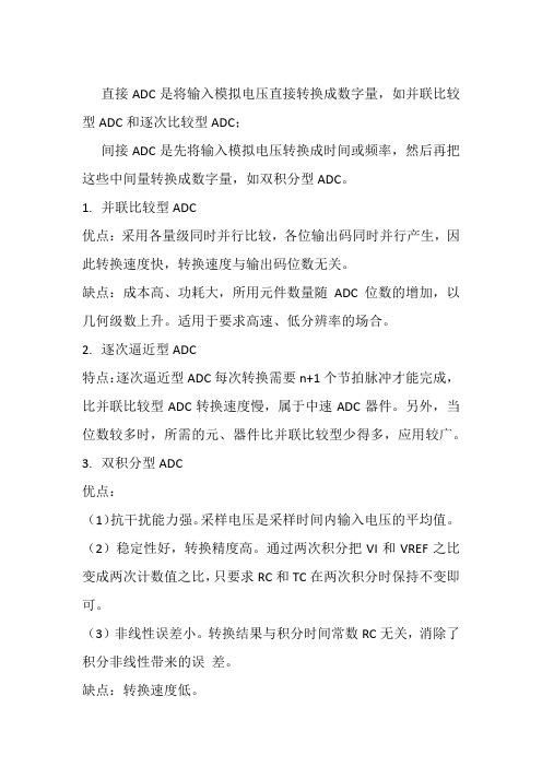
直接ADC是将输入模拟电压直接转换成数字量,如并联比较型ADC和逐次比较型ADC;
间接ADC是先将输入模拟电压转换成时间或频率,然后再把这些中间量转换成数字量,如双积分型ADC。
1.并联比较型ADC
优点:采用各量级同时并行比较,各位输出码同时并行产生,因此转换速度快,转换速度与输出码位数无关。
缺点:成本高、功耗大,所用元件数量随ADC位数的增加,以几何级数上升。
适用于要求高速、低分辨率的场合。
2.逐次逼近型ADC
特点:逐次逼近型ADC每次转换需要n+1个节拍脉冲才能完成,比并联比较型ADC转换速度慢,属于中速ADC器件。
另外,当位数较多时,所需的元、器件比并联比较型少得多,应用较广。
3.双积分型ADC
优点:
(1)抗干扰能力强。
采样电压是采样时间内输入电压的平均值。
(2)稳定性好,转换精度高。
通过两次积分把VI和VREF之比变成两次计数值之比,只要求RC和TC在两次积分时保持不变即可。
(3)非线性误差小。
转换结果与积分时间常数RC无关,消除了积分非线性带来的误差。
缺点:转换速度低。
常用的几种类型的ADC基本原理及特点
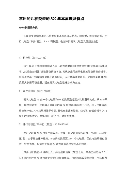
常用的几种类型的ADC基本原理及特点AD转换器的分类下面简要介绍常用的几种类型的基本原理及特点:积分型、逐次逼近型、并行比较型/串并行型、Σ-Δ调制型、电容阵列逐次比较型及压频变换型。
1)积分型(如TLC7135)积分型AD工作原理是将输入电压转换成时间(脉冲宽度信号)或频率(脉冲频率),然后由定时器/计数器获得数字值。
其优点是用简单电路就能获得高分辨率,但缺点是由于转换精度依赖于积分时间,因此转换速率极低。
初期的单片AD转换器大多采用积分型,现在逐次比较型已逐步成为主流。
2)逐次比较型(如TLC0831)逐次比较型AD由一个比较器和DA转换器通过逐次比较逻辑构成,从MSB开始,顺序地对每一位将输入电压与内置DA转换器输出进行比较,经n次比较而输出数字值。
其电路规模属于中等。
其优点是速度较高、功耗低,在低分辩率(<12位)时价格便宜,但高精度(>12位)时价格很高。
3)并行比较型/串并行比较型(如TLC5510)并行比较型AD采用多个比较器,仅作一次比较而实行转换,又称FLash(快速)型。
由于转换速率极高,n位的转换需要2n-1个比较器,因此电路规模也极大,价格也高,只适用于视频AD转换器等速度特别高的领域。
串并行比较型AD结构上介于并行型和逐次比较型之间,最典型的是由2个n/2位的并行型AD转换器配合DA转换器组成,用两次比较实行转换,所以称为Half flash(半快速)型。
还有分成三步或多步实现AD转换的叫做分级(Multistep/Subrangling)型AD,而从转换时序角度又可称为流水线(Pipelined)型AD,现代的分级型AD中还加入了对多次转换结果作数字运算而修正特性等功能。
这类AD速度比逐次比较型高,电路规模比并行型小。
4)Σ-Δ(Sigma/FONT>del ta)调制型(如AD7705)Σ-Δ型AD由积分器、比较器、1位DA转换器和数字滤波器等组成。
第15章-模拟数字转换器ADC(自学内容)

外部触发转换选用通用定时器1的捕获比较器2
ADC_ExternalTrigConv_T1_CC2
外部触发转换选用通用定时器1的捕获比较器1
ADC_ExternalTrigConv_T1_CC1
描述
ADC_ExternalTrigConv
ADC_ScanConvMode 参数指定 ADC 工作在扫描模式(多通道)还是单次(单通道)模式。如果设置为 ENABLE ,就是扫描模式,设置 DISABLE 就是单次模式. ADC_ContinuousConvMode 参数指定转换是连续的还是单次的。如设置 ENABLE 就是连续的,设置 DISABLE 是单次的. ADC_NbrOfChannel 参数指定使用序列规则组中 ADC 通道的数目. 可以取 1 到 16. ADC_DataAlign 参数指定数据对齐方式.
函数原形
ADC_InitTypeDef 结构: 该结构定义在 stm32f10x_adc.h 文件中。 typedef struct { u32 ADC_Mode; FunctionalState ADC_ScanConvMode; FunctionalState ADC_ContinuousConvMode; u32 ADC_ExternalTrigConv; u32 ADC_DataAlign; u8 ADC_NbrOfChannel; } ADC_InitTypeDef
三、校准 ADC有一个内置自校准模式。校准可大幅减小因内部电容器组的变化而造成的准精度误差。 通过设置ADC_CR2寄存器的CAL位启动校准。一旦校准结束,CAL位被硬件复位,可以开始正常转换。 注意: 1、建议在每次上电后执行校准。 2、启动校准前,ADC必须处于关电状态(ADON=’0’)超过至少两个ADC时钟周期。
adc的种类,工作原理和用途

adc的种类,工作原理和用途ADC(Analog-to-Digital Converter,模拟-数字转换器)是一种将连续的模拟信号转换为离散的数字信号的设备。
在现代电子系统中,ADC起着至关重要的作用。
本文将介绍ADC的种类、工作原理和用途。
一、ADC的种类1.并行ADC:并行ADC(Parallel ADC)是一种高速、高精度的转换器。
它将多个转换单元并行工作,以提高整体转换速度。
并行ADC适用于高速数据采集和实时信号处理场景。
2.串行ADC:串行ADC(Serial ADC)是一种低速、低精度的转换器。
它通过串行传输数据,逐位完成模拟信号到数字信号的转换。
串行ADC适用于对速度要求不高的场景,如通信系统和传感器信号处理。
3.流水线ADC:流水线ADC(Pipeline ADC)是一种高效的多级转换器。
它将整个转换过程分为多个阶段,每个阶段按照一定顺序依次完成。
流水线ADC能够在较低的时钟频率下实现高速转换。
4.积分式ADC:积分式ADC(Integrating ADC)是一种基于积分原理的转换器。
它通过测量输入信号与参考信号的积分差值,实现模拟信号到数字信号的转换。
积分式ADC具有高精度和低漂移的特点。
5.闪烁ADC:闪烁ADC(Flash ADC)是一种高速、高精度的转换器。
它利用多个并行转换单元,在纳秒级时间内完成模拟信号的转换。
闪烁ADC适用于高性能数据采集和实时信号处理。
二、ADC的工作原理1.采样:ADC通过采样定理确定采样频率,将高速变化的模拟信号转换为离散的数字信号。
采样定理指出,采样频率必须大于信号带宽的2倍,以确保信号的完整性。
2.量化:采样后的模拟信号需要进行量化,将其转换为二进制数字序列。
量化的过程通常采用均匀量化或非均匀量化方法。
3.编码:量化后的二进制数字序列需要进行编码,以便存储和传输。
常用的编码方式有努塞尔编码、韦弗编码等。
4.转换:ADC将编码后的二进制数字序列转换为数字信号,从而实现模拟信号到数字信号的转换。
ADC

SPECIFICATION1. 模数转换技术(概述)模数转换包括采样、保持、量化、编码四个过程。
采样就是将一个连续变化的信号X(t)转换成时间上离散的采样信号X(n)。
根据奈奎斯特采样定理,对于采样(t)信号X(t),如果采样频率fs大于或等于2fmax(fmax为X(t)最高频率成分,则可以无失真地重建恢复原始信号。
实际上,由于模数转换器器件的非线性失真,量化噪声及接收机噪声等因素的影响,采样速率一般取fs=2.5fmax 。
通常采样脉冲的宽度TW是很短的,故采样输出是断续的窄脉冲。
要把一个采样输出信号数字化,需要将采样输出所得的瞬时模拟信号保持一段时间,这就是保持过程。
量化是将连续幅度的抽样信号转换成离散时间、离散幅度的数字信号,量化的主要问题就是量化误差。
假设噪声信号在量化电平中是均匀分布的,则量化噪声均方值与量化间隔和模数转换器的输入阻抗值有关。
编码是将量化后的信号编码成二进制代码输出。
2. ADC的种类(1)传统型:积分型ADC(低速),逐次逼近型ADC(中速),并行ADC(高速)(2)其它型:中速:pipeline algorithmic ADC 高速:interpolating ADC folding ADC two-step ADCmultiple-bit pipeline ADCtime-iterleaved ADC高性能:delta-sigma ADC(中高速)3. 主要性能要求(1)高速参考速度10MHz—165MHz(采样频率)估算需要50MHz—80MHz(2)精度分辨率8位,10位(各一个)(3)高动态范围(4)低功耗(5)低噪声(6)面积小4. 不同种类的ADC工作原理及性能简述(1)积分型(dual-slope)ADC:积分型模数转换器[图1]包含积分器、比较器、计数器、时钟发生器和一些控制逻辑。
转换开始前,积分器的输出电压为0伏,计数器的状态为0,转换开始后,积分器对输入电压进行积分,其输出电压线性下降。
adc 采样电容的 结构类型
adc 采样电容的结构类型
ADC(模数转换器)采样电容的结构类型主要有以下几种:
1. 陶瓷电容:陶瓷电容具有高介电常数、低等效串联电阻(ESR)和低成本等优点,适用于高精度和高频率的ADC采样。
2. 薄膜电容:薄膜电容具有低ESR、低漏电流、高绝缘电阻和良好的温度稳定性等优点,适用于高精度和高稳定的ADC采样。
3. 电解电容:电解电容具有高电容量、低ESR和低成本等优点,适用于低精度、大电流和高电压的ADC采样。
4. 电感电容(LC)滤波器:LC滤波器由一个电感和一个电容组成,用于将输入信号的频率分量滤除,只保留所需的频率分量,适用于频率选择性和抗干扰性要求较高的ADC采样。
5. 集成电容:集成电容是将多个电容集成在一个芯片上,具有体积小、成本低、可靠性高等优点,适用于需要高密度和小型化的ADC采样。
不同的结构类型适用于不同的应用场景,需要根据具体需求选择合适的结构类型。
ADC种类及参数选择

ADC的分类特性和参数选择尽管A/D转换器的种类很多,但目前广泛应用的主要有:逐次逼近式A/D转换器、双积分式A/D转换器、V/F变换式A/D转换器,新型的Σ-Δ型A/D转换器。
逐次逼近寄存器型(SAR)模拟数字转换器(ADC)是采样速率低于5Msps (每秒百万次采样)的中等至高分辨率应用的常见结构。
SAR ADC的分辨率一般为8位至16位,具有低功耗、小尺寸等特点。
这些特点使该类型ADC具有很宽的应用范围,例如便携/电池供电仪表、笔输入量化器、工业控制和数据/信号采集等。
顾名思义,SAR ADC实质上是实现一种二进制搜索算法。
所以,当内部电路运行在数兆赫兹(MHz)时,由于逐次逼近算法的缘故,ADC采样速率仅是该数值的几分之一。
SAR ADC的架构:尽管实现SAR ADC的方式千差万别,但其基本结构非常简单(见图1)。
模拟输入电压(VIN)由采样/保持电路保持。
为实现二进制搜索算法,N位寄存器首先设置在中间刻度(即:100... .00,MSB设置为1)。
这样,DAC输出(VDAC)被设为VREF/2,VREF是提供给ADC的基准电压。
然后,比较判断VIN是小于还是大于VDAC。
如果VIN大于VDAC,则比较器输出逻辑高电平或1,N位寄存器的MSB保持为1。
相反,如果VIN小于VDAC,则比较器输出逻辑低电平,N位寄存器的MSB清0。
随后,SAR控制逻辑移至下一位,并将该位设置为高电平,进行下一次比较。
这个过程一直持续到LSB。
上述操作结束后,也就完成了转换,N位转换结果储存在寄存器内。
图1. 简单的N位SAR ADC架构图2给出了一个4位转换示例,y轴(和图中的粗线)表示DAC的输出电压。
本例中,第一次比较表明VIN < VDAC。
所以,位3置为0。
然后DAC被置为01002,并执行第二次比较。
由于VIN > VDAC,位2保持为1。
DAC置为01102,执行第三次比较。
根据比较结果,位1置0,DAC又设置为01012,执行最后一次比较。
- 1、下载文档前请自行甄别文档内容的完整性,平台不提供额外的编辑、内容补充、找答案等附加服务。
- 2、"仅部分预览"的文档,不可在线预览部分如存在完整性等问题,可反馈申请退款(可完整预览的文档不适用该条件!)。
- 3、如文档侵犯您的权益,请联系客服反馈,我们会尽快为您处理(人工客服工作时间:9:00-18:30)。
模数转换器(ADC)的几种主要类型
现在的软件无线电、数字图像采集都需要有高速的A/D采样保证有效性和精度,一般的测控系统也希望在精度上有所突破,人类数字化的浪潮推动了A/D转换器不断变革,而A/D转换器是人类实现数字化的先锋。
A/D转换器发展了30多年,经历了多次的技术革新,从并行、逐次逼近型、积分型ADC,到近年来新发展起来的∑-Δ型和流水线型ADC,它们各有其优缺点,能满足不同的应用场合的使用。
逐次逼近型、积分型、压频变换型等,主要应用于中速或较低速、中等精度的数据采集和智能仪器中。
分级型和流水线型ADC主要应用于高速情况下的瞬态信号处理、快速波形存储与记录、高速数据采集、视频信号量化及高速数字通讯技术等领域。
此外,采用脉动型和折叠型等结构的高速ADC,可应用于广播卫星中的基带解调等方面。
∑-Δ型ADC主应用于高精度数据采集特别是数字音响系统、多媒体、地震勘探仪器、声纳等电子测量领域。
下面对各种类型的ADC作简要介绍。
1.逐次逼近型
逐次逼近型ADC是应用非常广泛的模/数转换方法,它包括1个比较器、1个数模转换器、1个逐次逼近寄存器(SAR)和1个逻辑控制单元。
它是将采样输入信号与已知电压不断进行比较,1个时钟周期完成1位转换,N位转换需要N个时钟周期,转换完成,输出二进制数。
这一类型ADC的分辨率和采样速率是相
互矛盾的,分辨率低时采样速率较高,要提高分辨率,采样速率就会受到限制。
优点:分辨率低于12位时,价格较低,采样速率可达1MSPS;与其它ADC相比,功耗相当低。
缺点:在高于14位分辨率情况下,价格较高;传感器产生的信号在进行模/数转换之前需要进行调理,包括增益级和滤波,这样会明显增加成本。
2.积分型ADC
积分型ADC又称为双斜率或多斜率ADC,它的应用也比较广泛。
它由1个带有输入切换开关的模拟积分器、1个比较器和1个计数单元构成,通过两次积分将输入的模拟电压转换成与其平均值成正比的时间间隔。
与此同时,在此时间间隔内利用计数器对时钟脉冲进行计数,从而实现A/D转换。
积分型ADC两次积分的时间都是利用同一个时钟发生器和计数器来确定,因此所得到的D表达式与时钟频率无关,其转换精度只取决于参考电压VR。
此外,由于输入端采用了积分器,所以对交流噪声的干扰有很强的抑制能力。
能够抑制高频噪声和固定的低频干扰(如50Hz或60Hz),适合在嘈杂的工业环境中使用。
这类ADC主要应用于低速、精密测量等领域,如数字电压表。
优点:分辨率高,可达22位;功耗低、成本低。
缺点:转换速率低,转换速率在12位时为100~300SPS。
3.并行比较A/D转换器
并行比较ADC主要特点是速度快,它是所有的A/D转换器中速度最快的,现代发展的高速ADC大多采用这种结构,采样速率能达到1GSPS以上。
但受到功率和体积的限制,并行比较ADC的分辨率难以做的很高。
这种结构的ADC所有位的转换同时完成,其转换时间主取决于比较器的开关速度、编码器的传输时间延迟等。
增加输出代码对转换时间的影响较小,但随着分辨率的提高,需要高密度的模拟设计以实现转换所必需的数量很大的精密分压电阻和比较器电路。
输出数字增加一位,精密电阻数量就要增加一倍,比较器也近似增加一倍。
并行比较ADC的分辨率受管芯尺寸、输入电容、功率等限制。
结果重复的并联比较器如果精度不匹配,还会造成静态误差,如会使输入失调电压增大。
同时,这一类型的ADC由于比较器的亚稳压、编码气泡,还会产生离散的、不精确的输出,即所谓的“火花码”。
优点:模/数转换速度最高。
缺点:分辨率不高,功耗大,成本高。
4.压频变换型ADC
压频变换型ADC是间接型ADC,它先将输入模拟信号的电压转换成频率与其成正比的脉冲信号,然后在固定的时间间隔内对此脉冲信号进行计数,计数结果即为正比于输入模拟电压信号的数字量。
从理论上讲,这种ADC的分辨率可以无限增加,只要采用时间长到满足输出频率分辨率要求的累积脉冲个数的宽度即可。
优点:精度高、价格较低、功耗较低。
缺点:类似于积分型ADC,其转换速率受到限制,12位时为100~300SPS。
5.∑-Δ型ADC
∑-Δ转换器又称为过采样转换器,它采用增量编码方式即根据前一量值与后一量值的差值的大小来进行量化编码。
∑-Δ型ADC包括模拟∑-Δ调制器和数字抽取滤波器。
∑-Δ调制器主要完成信号抽样及增量编码,它给数字抽取滤波器提供增量编码即∑-Δ码;数字抽取滤波器完成对∑-Δ码的抽取滤波,把增量编码转换成高分辨率的线性脉冲编码调制的数字信号。
因此抽取滤波器实际上相当于一个码型变换器。
优点:分辨率较高,高达24位;转换速率高,高于积分型和压频变换型ADC;价格低;内部利用高倍频过采样技术,实现了数字滤波,降低了对传感器信号进行滤波的要求。
缺点:高速∑-△型ADC的价格较高;在转换速率相同的条件下,比积分型和逐次逼近型ADC的功耗高。
6.流水线型ADC
流水线结构ADC,又称为子区式ADC,它是一种高效和强大的模数转换器。
它能够提供高速、高分辨率的模数转换,并且具有令人满意的低功率消耗和很小的芯片尺寸;经过合理的设计,还可以提供优异的动态特性。
流水线型ADC由若干级级联电路组成,每一级包括一个采样/保持放大器、一个低分辨率的ADC和DAC以及一个求和电路,其中求和电路还包括可提供增益的级间放大器。
快速精确的n位转换器分成两段以上的子区(流水线)来完成。
首级电路的采样/保持器对输入信号取样后先由一个m位分辨率粗A/D转换器对输入进行量化,接着用一个至少n位精度的乘积型数模转换器(MDAC)产生一个对应于量化结果的模/拟电平并送至求和电路,求和电路从输入信号中扣除此模拟电平。
并将差值精确放大某一固定增益后关交下一级电路处理。
经过各级这样的处理后,最后由一个较高精度的K位细A/D转换器对残余信号进行转换。
将上述各级粗、细A/D的输出组合起来即构成高精度的n位输出。
优点:有良好的线性和低失调;可以同时对多个采样进行处理,有较高的信号处理速度,典型的为Tconv<100ns;低功率;高精度;高分辨率;可以简化电路。
缺点:基准电路和偏置结构过于复杂;输入信号需要经过特殊处理,以便穿过数级电路造成流水延迟;对锁存定时的要求严格;对电路工艺要求很高,电路板上设计得不合理会影响增益的线性、失调及其它参数。
目前,这种新型的ADC结构主要应用于对THD和SFDR及其它频域特性要求较高的通讯系统,对噪声、带宽和瞬态相应速度等时域特性要求较高的CCD成像系统,对时域和频域参数都要求较高的数据采集系统。