(完整)SPSS实验指导手册(定稿)
SPSS和SAS统计实验指导书

实用标准文档SPSS和SAS统计实验指导书(学生用)王慧、欧晓华、王立平等编经济与贸易系市场营销教研室2006年4月目录实验一:统计描述 (3)1.均值(Mean)和均值标准误差(S.E.mean) (3)2.中位数(Median) (5)3.众数(Mode) (6)4.全距(Range) (7)5.方差(Variance)和标准差(Standard Deviation) (8)6.四分位数(Quartiles)和十分位数(Deciles) (10)7.频数(Frequency) (12)8.峰度(Kurtosis) (14)9.偏度(Skewness) (16)实验二:均值比较和T检验 (17)1.均值比较 (17)2.单一样本T检验 (20)3.两独立样本T检验 (21)4.两配对样本T检验 (23)实验三:相关分析 (26)1.实验理论概述 (26)2.二元定距变量的相关分析 (26)3.二元定序变量的相关分析 (33)4.偏相关分析 (36)5.距离相关分析 (41)实验四:回归分析 (51)1.一元线性回归 (51)2.多元线性回归分析 (57)实验一:统计描述实验内容:均值、中位数、众数、全距、方差与标准差、四分位数、十分位数、频数、峰度、偏度实习目的:掌握SPSS基本的统计描述方法,可以对要分析的数据的总体特征有比较准确的把握,从而为以后实验项目选择其他更为深入的统计分析方法打下基础。
实验一要研究的问题:输入SPSS保存。
1.均值(Mean)和均值标准误差(S.E.mean)问题:求该班级在一次数学测验中的平均成绩和其标准差★实验步骤:『步骤1』单击“Analyze”菜单“Descriptive statistics”项中的“Frequencies”命令,如图1-1所示。
图1-1 选择Frequencies菜单『步骤2』弹出Frequencies对话框,如图1-2所示,在对话框左侧的便利列表中选择“数学”,单击按钮使之添加到Variable(s)框中。
SPSS实验指导书(全)

《SPSS统计软件应用》实验指导书目录1.实验一 SPSS的数据管理2.实验二描述性统计分析3.实验三均值检验4.实验四相关分析5.实验五因子分析6.实验六聚类分析7.实验七回归分析8.实验八判别分析实验一SPSS的数据管理一、实验目的1.熟悉SPSS的菜单和窗口界面,熟悉SPSS各种参数的设置;2.掌握SPSS的数据管理功能。
二、实验内容及步骤统计分析离不开数据,因此数据管理是SPSS的重要组成部分。
详细了解SPSS 的数据管理方法,将有助于用户提高工作效率。
SPSS的数据管理是借助于数据管理窗口和主窗口的File、Data、Transform等菜单完成的。
(一) SPSS进行统计处理的基本过程SPSS是Statistics Package for Social Sciences(社会科学统计软件包)的缩写,被广泛应用于社会科学和自然科学的各个领域中。
SPSS功能强大,但操作简单,这一特点突出地体现在它统一而简单的使用流程中。
SPSS进行统计处理的基本过程如图6-1所示:其基本步骤如下:1. 数据的录入将数据以电子表格的方式输入到SPSS中(*.sav, 是SPSS独有的格式),也可以从其它可转换的数据文件中读出数据。
数据录入的工作分两个步骤,一是定义变量,二是录入变量值。
2. 数据的预分析在原始数据录入完成后,要对数据进行必要的预分析,如数据分组、排序、分布图、平均数、标准差的描述等,以掌握数据的基本特点和基本情况,保证后续工作的有效性,也为确定应采用的统计检验方法提供依据。
3. 统计分析按研究的要求和数据的情况确定统计分析方法,然后对数据进行统计分析。
4. 统计结果可视化在统计过程进行完后,SPSS会自动生成一系列数据表,其中包含了统计处理产生的整套数据。
为了能更形象地呈现数据,需要利用SPSS提供的图形生成工具将所得数据可视化。
如前所述,SPSS提供了许多图形来进行数据的可视化处理,使用时可根据数据的特点和研究的需求来进行选择。
SPSS实验手册

PASW统计分析方法与应用(实验手册)北京师范大学管理学院2010年3月Experiment 1:Creating and Editing a Data File1. Set up the variables described above for the grades.sav file, using appropriate variable names,variable labels, and variable values. Enter the data for the first five students into the data file.2. Perhaps the instructor of the classes in the grades.sav dataset teaches these classes at two different schools. Create a new variable in this dataset named school, with values of 1 and 2. Create variable labels, where 1 is the name of a school you like, and 2 is the name of a school you don’t like. Save your dataset with the name gradesme.sav.3. Which of the following variable names will SPSS accept, and which will SPSS reject? For those that SPSS will reject, how could you change the variable name to make it “legal”?agefirstname@edusex.gradenotanxeceudateiq4. Using the grades.sav file, make the gpa variable values (which currently have two digits after the decimal place) have no digits after the decimal point. You should be able to do this without retyping any numbers. Note that this won’t actually round the numbers, but it will change the way they are displayed and how many digits are displayed after the decimal point for statistical analyses you perform on the numbers.5. Using grades.sav, search for a student who got 121 on the final exam. What is his or her name?6. Why is each of the following variables defined with the measure listed? Is it possible for any of these variables to be defined as a different type of measure?ethnicity Nominalextrcred Ordinalquiz4 Scalegrade Nominal7. Ten people were given a test of balance while standing on level ground, and ten other people were given a test of balance while standing on a 30° slope. Their scores follow. Set up the appropriate variables, and enter the data into SPSS.Scores of people standing on level ground: 56, 50, 41, 65, 47, 50, 64, 48, 47, 57 Scores of people standing on a slope: 30, 50, 51, 26, 37, 32, 37, 29, 52, 548. Ten people were given two tests of balance, first while standing on level ground and then whilestanding on a 30° slope. Their scores follow. Set up the appropriate variables, and enter the datainto SPSS.Participant: 1 2 3 4 5 6 7 8 9 10Score standing on level ground: 56 50 41 65 47 50 64 48 47 57Score standing on a slope: 38 50 46 46 42 41 49 38 49 55Experiment 2:Managing DataSome of the exercises that follow change the original data file. If you wish to leave the data in their original form, don’t save your changes.Case Summaries1. Using the grades.sav file, list variables (in the original order) from id to quiz5, first 30 students consecutive, number cases, fit on one page by editing.2. Using the helping3.sav file, list variables hclose, hseveret, angert, hcontrot, sympathi, worry, obligat, hcopet, first 30 cases, number cases, fit on one page by editing.3. List the first 20 students in the grades.sav file, with the lower division students listed first, followed by the upper division students.Missing Values4. Using the grades.sav file delete the quiz1 scores for the cases selected in exercise 3, above. Replace the (now) missing scores with the average score for all other students in the class.Computing Variables5. Now that you have changed the quiz1 scores (in exercise 4), recalculate total (the sum of all five quizzes and the final) and percent (100 times the total divided by the points possible, 125).6. Using the divorce.sav file compute a variable named spirit (spirituality) that is the mean of sp8 through sp57 (there should be 18 of them). Print out id, sex, and the new variable spirit, first 30 cases, edit to fit on one page.7. Using the grades.sav file, compute a variable named quizsum that is the sum of quiz1 through quiz5. Print out variables id, lastname, firstnam, and the new variable quizsum, first 30, all on one page.Recode Variables8. Using the grades.sav file, compute a variable named grade2 according to the instructions on page 55. Print out variables id, lastname, firstnam, grade and the new variable grade2, first 30, edit to fit all on one page. If done correctly, grade and grade2 should be identical.9. Recode the passfail variable so that D’s and F’s are failing, and A’s, B’s, and C’s are passing.ing the helping3.sav file, redo the coding of the ethnic variable so that Black = 1, Hispanic = 2,Asian = 3, Caucasian = 4, and Other/DTS = 5. Now change the value labels to be consistent with reality (that is the coding numbers are different but the labels are consistent with the original ethnicity). Print out the variables id and ethnic, first 30 cases.Selecting Casesing the divorce.sav file select females (sex = 1); print out id and sex, first 40 subjects, numbered,fit on one page.12. Select all of the students in the grades.sav file whose previous GPA’s are less than 2, and whose percent ages for the class is greater than 85.13. Using the helping3.sav file, select females (gender = 1) who give more than the average amount of help (thelplnz > 0). Print out id, gender, thelplnz, first 40 subjects, numbered, fit on one page.Sorting Cases14.Alphabetize the grades.sav file by lastname, firstnam, first 40 cases.ing the grades.sav file, sort by id (ascending order). Print out id, total, percent, and grade, first 40 subjects, fit on one page.Experiment 3:GraphsAll of the following exercises use the grades.sav sample data file.1. Using a bar chart, examine the number of students in each section of the class along with whether or not student attended the review session. Does there appear to be a relation between these variables?2. Using a line graph, examine the relationship between attending the review session and section on the final exam score. What does this relationship look like?3. Create a boxplot of quiz 1 scores. What does this tell you about the distribution of the quiz scores?Create a boxplot of quiz 2 scores. How does the distribution of this quiz differ from the distribution of quiz 1? Which case number is the outlier?4. Create an error bar graph highlighting the 95% confidence interval of the mean for each of the three section s’ final exam scores. What does this mean?5. Based on the examination of a histogram, does it appear that students’ previous GPA’s are normally distributed?6. Create the scatterplot described in Step 5g. What does the relationship appear to be between gender and academic performance (total)? Add a regression line to this scatterplot. What does this regression line tell you?Experiment 4:Frequencies1. Using the divorce.sav file display frequencies for sex, eth, status. Print output to show frequencies for all three; edit output so it fits on one page. Include three bar graphs of these data and provide labels to clarify what each one means.2. Using the graduate.sav file display frequencies for motiv, stable, hostile. Print output to show frequencies for all three; edit output so it fits on one page. Note: this type of procedure is typically done to check for accuracy of data. Motivation (motiv), emotional stability (stable), and hostility (hostile) are scored on 1 to 7 scales. You are checking to see if you have, by mistake, entered any 0s or 8s or 77s.3. Using the helping3.sav file compute percentiles for thelplnz (time helping, measured in z scores), tqualitz (quality of help measured in z scores). Use percentile values 2, 16, 50, 84, 98. Print output and circle values associated with percentiles for thelplnz; box percentile values for tqualitz.4. Using the helping3.sav file compute percentiles for age. Compute every 10th percentile (10, 20, 30, etc.). Edit (if necessary) to fit on one page.5. Using the graduate.sav file display frequencies for gpa, areagpa, grequant. Compute quartiles for these three variables. Edit (if necessary) to fit on one page.6. Using the grades.sav file create a histogram for final. Create a title for the graph that makes clear what is being measured.Experiment 5:Descriptive Statistics1. Using the grades.sav file select all variables except lastname, firstname, grade, passfail. Compute descriptive statistics including mean, standard deviation, kurtosis, skewness. Edit so that you eliminate “S.E. Kurt” and “S.E. Skew” and your chart is easier to interpret, and the output fits on one page.Draw a line through any variable for which descriptives are meaningless (either they are categorical or they are known to not be normally distributed)Place an “*” next to variables that are in the ideal range for both skewness and kurtosisPlace an × next to variables that are acceptable but not excellentPlace a ψ next to any variables that are not acceptable for further analysis2. Using the divorce.sav file select all variables except the indicators (for spirituality, sp8 – sp57, for cognitive coping, cc1 – cc11, for behavioral coping, bc1 – bc12, for avoidant coping, ac1 – ac7, and for physical closeness, pc1 – pc10). Compute descriptive statistics including mean, standard deviation, kurtosis, skewness. Edit so that you eliminate “S.E. Kurt” and “S.E. Skew” and your chart is easier to interpret, and the output fits on two pages.Draw a line through any variable for which descriptives are meaningless (either they are categorical or they are known to not be normally distributed)Place an “*” next to variables that are in the ideal range for both skewness and kurtosisPlace an × next to variables that are acceptable but not excellentPlace a ψ next to any variables that are not acceptable for further analysis3. Create a practice data file that contains the following variables and values:VAR1: 3 5 7 6 2 1 4 5 9 5VAR2: 9 8 7 6 2 3 3 4 3 2VAR3: 10 4 3 5 6 5 4 5 2 9Compute: the mean, the standard deviation, and variance and print out on a single page.Experiment 5:Crosstabulation and χ2 AnalysesFor each of the chi-square analyses computed below:1. Circle the observed (actual) values.2. Box the expected values.3. Put an * next to the unstandardized residuals.4. Underline the significance value that shows whether observed and expected values differ significantly.5. Make a statement about independence of the variables involved.6. STATE THE NATURE OF THE RELATIONSHIP (in normal English, not statistical jargon).7. Is there a significant linear association?8. Does linear association make sense for these variables?9. Is there a problem with low-count cells?10.What would you do about it if there is a problem?1. File: grades.sav. Variables: gender by ethnicity. Select: observed count, expected count, unstandarized residuals; Compute: Chi-square, Phi and Cramer’s V; edit to fit on one page; print out; perform the 10 operations above.2. File: grades.sav. Variables: gender by ethnicity. Prior to analysis, complete the procedure shown in Step 5c (page 111) to eliminate the “Native” category (due to too many low-count cells). Select: observed count, expected count, unstandarized residuals; Compute: Chi-square, Phi and Cramer’s V; edit to fit on one page; print out; perform the 10 operations listed above.3. File: helping3.sav. Variables: gender by problem. Select: observed count, expected count, unstandarized residuals; Compute: Chi-square, Phi and Cramer’s V; edit to fit on one page; print out; perform the 10 operations.4. File: helping3.sav. Variables: school by occupat. Prior to analysis, select cases: “school > 1 & occupat < 6”. Select: observed count, expected count, unstandarized residuals; Compute: Chi-square, Phi and Cramer’s V; edit to fit on one page; print out; perform the 10 operations above.5. File: helping3.sav. Variables: marital by problem. Select: observed count, expected count, unstandarized residuals; Compute: Chi-square, Phi and Cramer’s V; edit to fit on one page; print out; perform the 10 operations listed above.Experiment 6:Bivariate Correlation1. Using the grades.sav file create a correlation matrix of the following variables; id, ethnic, gender, year, section, gpa, quiz1, quiz2, quiz3, quiz4, quiz5, final, total; select one-tailed significance; flag significant correlations.Draw a single line through the columns and rows where the correlations are meaningless.Draw a double line through the correlations where there is linear dependency Circle 3 legitimate NEGATIVE correlations where the significance is p < .05 and explain what they mean.Box 3 legitimate POSITIVE correlations where the significance is p < .05 and explain what they mean.Create a scatterplot of gpa by total and include the regression line. (see Chapter5 for instructions).2. Using the divorce.sav file create a correlation matrix of the following variables; sex, age, sep, mar, status, eth, school, income, avoicope, iq, close, locus, asq, socsupp, spiritua, trauma, lsatisfy; select one-tailed significance; flag significant correlations. Note: Please make use of the Data Files descriptions starting on page 365 for meaning of all variables.Draw a single line through the columns and rows where the correlations are meaningless.Draw a double line through the correlations where there is linear dependency Circle 3 legitimate NEGATIVE correlations where the significance is p < .05 and explain what they mean.Box 3 legitimate POSITIVE correlations where the significance is p < .05 and explain what they mean.Create a scatterplot of close by lsatisfy and include the regression line. (see Chapter 5 for instructions).Create a scatterplot of avoicope by trauma and include the regression line.Experiment 7:The T Test ProcedureFor questions 1- 7, perform the following operations:a) Circle the two mean values that are being comparedb) Circle the appropriate significance value (be sure to consider equal or unequal variance)c) If the results are statistically significant, describe what the results mean.1. Using the grades.sav file, compare men with women (gender) for quiz1, quiz2, quiz3, quiz4, quiz5,final, total.2. Using the grades.sav file, determine whether the following pairings produce significant differences: quiz1 with quiz2, quiz1 with quiz3, quiz1 with quiz4, quiz1 with quiz5.3. Using the grades.sav file, compare the GPA variable (gpa) with the mean GPA of the university of 2.89.4. Using the divorce.sav file, compare men with women (sex) for lsatisfy, trauma, age, school, cogcope, behcope, avoicope, iq, close, locus, asq, socsupp, spiritua.5. Using the helping3.sav file, compare men with women (gender) for age, school, income, tclose, hcontrot, sympathi, angert, hcopet, hseveret, empathyt, effict, thelplnz, tqualitz, tothelp. Please see the Data Files section (page 365) for meaning of each variable.6. Using the helping3.sav file, determine whether the following pairings produce significant differences: sympathi with angert, sympathi with empathy, empahelp with insthelp, empahelp with infhelp, insthelp with infthelp.7. Using the helping3.sav file, compare the age variable (age) with the mean age for North Americans (33.0).8. In an experiment, 10 participants were given a test of mental performance in stressful situations. Their scores were 2, 2, 4, 1, 4, 3, 0, 2, 7, and 5. Ten other participants were given the same test after they had been trained in stress-reducing techniques. Their scores were 4, 4, 6, 0, 6, 5, 2, 3, 6, and 4. Do the appropriate t test to determine if the group that had been trained had different mental performance scores than the group that had not been trained in stress reduction techniques. What do these results mean?9. In a similar experiment, ten participants were given a test of mental performance in stressful situations at the start of the study, were then trained in stress reduction techniques, and were finally given the same test again at the end of the study. In an amazing coincidence, the participants received the same scores as the participants in question 8: The first two people in the study received a score of 2 on the pretest, and a score of 4 on the posttest; the third person received a score of 4 on the pretest and 6 on the posttest; and so on. Do the appropriate t test to determine if there was a significant difference between the pretest and posttest scores. What do these results mean? How was this similar and how was this different than the results in question 1? Why?10. You happen to know that the population mean for the test of mentalperformance in stressful situations is exactly three. Do a t test to determine whether the post test scores in #9 above (the same numbers as the training group scores in #8 above) is significantly different than three. What do these results mean? How was this similar and how was this different than the results in question 2? Why?Experiment 8:The One-Way ANOVA ProcedurePerform one-way ANOVAs with the specifications listed belowPerform one-way ANOVAs with the specifications listed below. If there are significant findings write them up in APA format (or in the professional format associated with your discipline). Examples of correct APA format are shown on the web site. Further, notice that the final five problems make use of the helping3.sav data file.1. File: grades.sav; dependent variable: quiz4; factor: ethnic (2,5); use LSD procedure for post hoc comparisons, compute two planned comparisons. Note that you will need to perform a select-cases procedure to delete the “1 =Native” category.APA Format:A one-way ANOVA revealed marginally significant ethnic differences for scores on Quiz 4, F(3, 96) = 2.27, p = .085. Post hoc comparisons using the LSD procedure with an alpha value of .05 found that Whites (M = 8.04) and Asians (M = 8.35) scored significantly higher than Hispanics (M = 6.27).2. File: helping3.sav; dependent variable: tothelp; factor: ethnic (1,4); use LSD procedure for post hoc comparisons, compute two planned comparisons.3. File: helping3.sav; dependent variable: tothelp; factor: problem (1,4); use LSD procedure for post hoc comparisons, compute two planned comparisons.4. File: helping3.sav; dependent variable: angert; factor: occupat (1,6); use LSD procedure for post hoc comparisons, compute two planned comparisons.5. File: helping3.sav; dependent variable: sympathi; factor: occupat (1,6); use LSD procedure for post hoc comparisons, compute two planned comparisons.6. File: helping3.sav; dependent variable: effict; factor: ethnic (1,4); use LSD procedure for post hoc comparisons, compute two planned comparisons.Experiment 9:Two-Way and Three-Way ANOVAFor the first five problems below, perform the following:Print out the cell means portion of the output.Print out the ANOVA results (main effects, interactions, and so forth).Interpret and write up correctly (APA format) all main effects and interactions. Create multiple-line graphs (or clustered bar charts) for all significant interactions .1. File: helping3.sav; dependent variable: tothelp; independent variables: gender, problem.APA Format:A 2-way ANOVA was conducted to determine the influence of gender and type of problem on the total amount of help given. Results showed a significant main effect for gender in which women (M = .12) gave more help than men (M = -.18), F(1, 529) = 5.54, p = .019. There was also a significant main effect for problem type, F(3, 529) = 1.65, p = .023. Post hoc comparisons using the least significant differences procedure with an alpha value of .05 revealed that subjects helping with a goal disruptive problem spent less time helping (M = -.12) than subjects helping with relational problems (M = .07) or illness problems (M = -.13). There was no significant gender by problem type interaction.2. File: helping3.sav; dependent variable: tothelp; independent variables: gender, income.3. File: helping3.sav; dependent variable: hseveret; independent variables: ethnic, problem.4. File: helping3.sav; dependent variable: thelplnz; independent variables: gender, problem;covariate: tqualitz.5. File: helping3.sav; dependent variable: thelplnz; independent variables: gender, income, marital.6. In an experiment, participants were given a test of mental performance in stressful situations. Some participants were given no stress-reduction training, some were given a short stress-reduction training session, and some were given a long stress-reduction training session. In addition, some participants who were tested had a low level of stress in their lives, and others had a high level of stress in their lives. Perform an ANOVA on these data (listed below).What do these results mean?7. In an experiment, participants were given a test of mental performance in stressful situations. Some participants were given no stress-reduction training, andsome were given a stress-reduction training session. In addition, some participants who were tested had a low level of stress in their lives, and others had a high level of stress in their lives. Finally, some participants were tested after a full night's sleep, and some were tested after an all-night study session on three-way ANOVA. Perform an ANOVA on these data (listed below question 8; ignore the "caffeine" column for now). What do these results mean?8.In the experiment described in problem 7, data were also collected for caffeine levels. Perform an ANOVA on these data (listed below). What do these results mean? What is similar to and different than the results in question 6?Experiment 10:Simple Linear Regression1. Use the anxiety.sav file exercises that followInclude output in as compact a form as is reasonableWrite the linear equation for the predicted exam scoreWrite the quadratic equation for the predicted exam scoreFor subjects numbered 5, 13, 42, and 45Substitute values into the two equations and solve. Show work on a separate page. Then compare in a small table (similar to that on page 182)Linear equation resultsQuadratic equation resultsActual scores for sake of comparison2. Now using the divorce.sav file, test for linear and curvilinear relations between: physical closeness (close) and life satisfaction (lsatisfy)attributional style (ASQ) and life satisfaction (lsatisfy)Print graphs and write linear and quadratic equations for both.3. Examine the relationship between exam score, anxiety and anxiety squared (from the anxiety.sav file) and similar procedures for the two relationships shown in problem 2 (from the divorce.sav file).For each of the three analyses:Box the Multiple RCircle the R SquareUnderline the two (2) B valuesDouble underline the two (2) Sig of T values.In a single sentence (just once, not for each of the 3 problems) identify the meaning of each of the four (4) bulleted items above.4. A researcher is examining the relationship between stress levels and performance on a test of cognitive performance. She hypothesizes that stress levels lead to an increase in performance to a point, and then increased stress decreases performance. She tests ten participants, who have the following levels of stress: 10.94, 12.76, 7.62, 8.17, 7.83, 12.22, 9.23, 11.17, 11.88, and 8.18. When she tests their levels of mental performance, she finds the following cognitive performance scores (listed in the same participant order as above):5.24, 4.64, 4.68, 5.04, 4.17,6.20, 4.54, 6.55, 5.79, and 3.17. Perform a linear regression to examine therelationship between these variables. What do these results mean?5. The same researcher tests ten more participants, who have the following levels of stress: 16, 20, 14, 21, 23, 19, 14, 20, 17, and 10. Their cognitive performance scores are (listed in the same participant order): 5.24, 4.64, 4.68, 5.04, 4.17,6.20, 4.54, 6.55, 5.79, and 3.17. (Note that in an amazing coincidence, these participants have the same cognitive performance scores as the participants in question 4; this coincidence may save you some typing.) Perform a linear regression to examine the relationship between these variables. What do these results mean?6. Create a scatterplot of the variables in question 5. How do results suggest that linear regression might not be the best analysis to perform?7. Perform curve estimation on the data from Question 5. What does this tell you about the data that you could not determine from the analysis in Question 5?8. What is different about the data in Questions 4 and 5 that leads to different results?Experiment 11:Multiple Linear RegressionUse the helping3.sav file for the exercises that follow.Conduct the following THREE regression analysis:Criterion variables:1. thelplnz: Time spent helping2. tqualitz: Quality of the help given3. tothelp: A composite help measure that includes both time and quality Predictors: (use the same predictors for each of the three dependent variables) age: range from 17 to 89angert: Amount of anger felt by the helper toward the needy friendeffict: Helper’s feeling of self-efficacy (competence) in relation to the friend’s problemempathyt: Helper’s empathic tendency as rated by a personality testgender: 1 = female, 2 = malehclose: Helper’s rating of how close the relationship washcontrot: helper’s rating of how controllable the cause of the problem was hcopet: helper’s rating of how well the friend was coping with his or her problem hseveret: helper’s rating of the severity of the problemobligat: the feeling of obligation the helper felt toward the friend in need school: coded from 1 to 7 with 1 being the lowest education, and 7 being the highest (> 19 years)sympathi: The extent to which the helper felt sympathy toward the friend worry: amount the helper worried about the friend in needUse entry value of .06 and removal value of .11.Use stepwise method of entry.Create a table (example below) showing for each of the three analyses Multiple R, R2, then each of the variables that significantly influence the dependent variables. Following the R2, List the name of each variable and then (in parentheses) list its β value. Rank order them from the most influential to least influential from left to right. Include only significant predictors.4. A researcher is examining the relationship between stress levels, self-esteem, coping skills, and performance on a test of cognitive performance (the dependent measure). His data are shown below. Perform multiple regression on these data, entering variables using the stepwise procedure. Interpret the results.Experiment 12:Reliability AnalysisUse the helping3.sav file for the exercises that follow. Measure the internal consistency (coefficient alpha) of the following sets of variables. An “h” in front of a variable name, refers to assessment by the help giver; an “r” in front of a variable name refers to assessment by the help recipient. Compute Coefficient alpha for the following sets of variables, then delete variables until you achieve the highest possible alpha value. Print out relevant results.1. hsevere1, hsevere2, rsevere1, rsevere2 measure of problem severity2. sympath1, sympath2, sympath3, sympath4 measure of helper’s sympathy3. anger1, anger2, anger3, anger4 measure of helper’s anger4. hcompe1, hcompe2, hcope3, rcope1, rcope2, rcope3 how well the recipient is coping5. hhelp1-hhelp15 helper’s rating of time spent helping6. rhelp1-rhelp15 recipient’s rating of time helping7. empathy1-empathy14 helper’s rating of empathy8. hqualit1, hqualit2, hqualit3, rqualit1, rqualit2, rqualit3 quality of help9. effic1-effic15 helper’s belief of self efficacy10. hcontro1, hcontro2, rcontro1, rcontro2 controllability of the cause of the problemFrom the divorce.sav file:11. drelat-dadjust (16 items) factors disruptive to divorce recovery12. arelat-amain2 (13 items) factors assisting recovery from divorce13. sp8-sp57 (18 items) spirituality measures。
新的!《SPSS统计分析》实验指导手册

对结果的简要分析:不同性别在购物因素的选择上存在着一定的差异,男性更多注意于服务质量,而女性更多关注于促销活动。
简介:SPSS统计分析方法的功能强大,应用广泛,熟悉这个软件是分析心理学各种实验数据的前提。
器材:PC机,多媒体设备
方法和程序:
1.SPSS的安装、启动、退出;
2.熟悉SPSS的各种结果浏览窗口、文本输出窗口。
实验二数据文件的建立与保存
目的:学会建立和保存一个SPSS数据文件,对一份心理学调查数据能正确地输入到SPSS文件中。
器材:PC机,多媒体设备
方法和程序:
以多选题.sav数据为例,对不同性别人群的购物因素进行交叉描述,并对不同性别的购物因素作简要分析。
分析:购物因素是一个多选题数据,首先需要设置多选题变量集:Multiple response—define sets—使用二分变量,取值为1,表示选中—输入变量集名称---把要进入变量集的各个变量进入variable in set—add—ok.
目的:通过操作使学生学会对数据进行必要的加工处理。
简介:对同一个数据往往要从各种不同的侧面进行研究,采取多种统计方法进行分析,而不同的统计方法对数据文件结构的要求不尽相同,这就需要对数据文件的结构进行重新调整或转换,以便适合于相应的统计方法,这项工作称为数据管理。
器材:PC机,多媒体设备
方法和程序:
6.根据多重比较的结果,三个类别教师两两之间均存在着显著差异,即新手-熟手-专家教师在教学策略水平上均存在着明显差异。
spss统计软件实验指导书(科大理学院)

统计软件实验指导书河南科技大学理学院统计学系2009年1月目录1.《统计软件实验教学大纲》2.实验一 SPSS基本操作3.实验二 SPSS数据录入与编辑4.实验三数据文件的整理5.实验四统计图的制作与编辑6.实验五基础统计分析7.实验六均值比较与T检验8.实验七单因素方差分析9.实验八多因素方差分析10.实验九两变量的相关分析11.实验十偏相关分析12.实验十一线性回归13.实验十二曲线拟合14.实验十三聚类分析15.实验十四判别分析16.实验十五因子分析17.实验十六非参数检验18.实验十七一个完整的社会统计分析19.实验十八操作考试20.实验报告书写格式课程代码:1010000940统计软件Statistical Software学分:3.5 总学时:72 理论学时:40 实验/实践学时:0/32面向专业:四年制统计学本科专业一、实验教学目标统计软件主要介绍了SPSS软件的应用,结合若干实例全面讲述了SPSS的基本操作功能、图形功能、统计分析功能。
学习本课程后,使学生能够依据数学原理,熟练操作SPSS软件进行统计分析,解决实际问题。
二、实验教学基本要求通过本课程的实验训练,要求达到:(1)掌握SPSS软件基本操作,包括SPSS基本特点和运行环境,SPSS中信息输入与输出,数据文件的编辑等比较基础的知识。
(2)掌握SPSS图形功能,包括二维、三维交互图。
(3)掌握SPSS统计分析功能,包括样本描述与数据准备、参数估计、假设检验、非参数检验、方差分析、回归分析、相关分析、因子分析、聚类分析、判别分析和可靠性分析等。
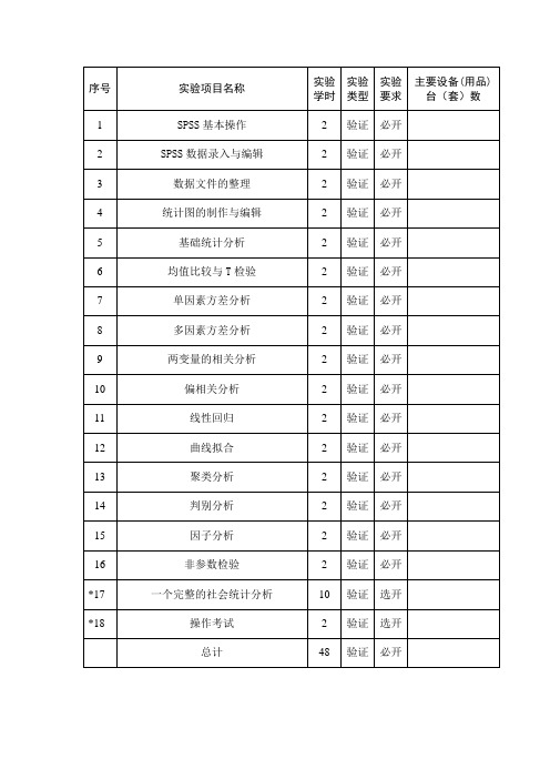
三、实验教材或实验指导书《SPSS统计分析从基础到实践》,罗应婷等主编,北京:电子工业出版社,2007年6月.四、考核方式与评分办法1.实验报告(40%)2.上机检查(40%)3. 上机考勤(20%)五、实验项目设置六、实验内容与实验方式实验方式1.由授课教师讲清上机实验的基本要求和注意事项;2.由授课教师事先布置上机实验的内容,设计要求,操作步骤,并要求学生课前进行准备;3.学生集中在机房上机;4.要求学生每次完成所布置的任务,提交实验报告。
spss实验指导书1
物流系统规划与仿真实验指导计划书一、实验目的实验是《物流系统规划》课程的重要教学环节,通过各种类型软件的仿真模拟和设计性实验教学环节,一方面增强学生解决实际问题的能力,以及加深对物流系统规划与设计的基本概念、基本原理和分析方法的理解,从而进一步激发学生利用物流系统规划与设计知识解决企业生产、管理、市场等问题的实际能力与创造力。
另一方面使学生了解物流系统规划与设计的流程与思想的具体应用,理解数学建模的方法,掌握物流系统软件的使用方法,拓宽学生的知识领域,增强对所学专业的热爱,激发学习的热情并明确学习目的。
二、实验要求(1)了解物流系统规划与建模的过程、方法及应用领域。
(2)掌握物流系统需求预测理论、线性规划理论、整数规划理论及路径规划理论。
(3)掌握统计分析软件SPSS的基本使用方法,并能进行基本的统计结果分析。
(4)掌握数学模型求解软件MathMatic基本的解析式求解方法。
(5)掌握物流规划与建模求解软件Lingo的基本使用方法,并能利用Lingo解决简单的物流优化问题。
三、实验时间、内容及考核标准1、实验时间:第16周——第18周2、实验内容及考核标准(1)实验一:SPSS软件概述实验目的:通过对SPSS软件的使用和讲解,让学生掌握SPSS软件的安装及基本使用功能。
实验课时:2课时实验要求:学习SPSS软件的安装、变量定义、数据录入、文件保存、SPSS绘图、数据预分析以及数据简单分析等基本使用功能。
考核标准:填写实验报告。
总结SPSS统计软件的使用方法,并完成以下实例:实例1:某克山病区测得11例克山病患者与13名健康人的血磷值(mmol/L)如下, 问该地急性克山病患者与健康人的血磷值是否不同?患者: 0.84 1.05 1.20 1.20 1.39 1.53 1.67 1.80 1.87 2.07 2.11健康人: 0.54 0.64 0.64 0.75 0.76 0.81 1.16 1.20 1.34 1.35 1.48 1.56 1.87实例2:某企业利润统计数据绘图。
SPSS实验手册

SPSS实验手册蔡鸣晶编南京信息职业技术学院目录实验一SPSS的数据管理 3 实验二频率分析 (7)实验三描述性分析 (8)实验四探索性分析 (9)实验五交叉表分析 (10)实验六SPSS创建图表 (12)实验七SPSS概率论初步 (14)实验八参数估计 (15)实验九假设检验 (16)附录一实验报告表格17 附录二实验报告样表16实验一 SPSS的数据管理一、实验目的与要求通过本实验,使学生理解并掌握SPSS软件包有关数据文件创建和整理的基本操作,学习如何将收集到的数据输入计算机,建成一个正确的SPSS数据文件,并掌握如何对原始数据文件进行整理,包括数据查询,数据修改、删除,数据的排序等等。
二、实验内容1、定义变量:试录入以下数据文件,并按要求进行变量定义,保存为“数据1-1.sav”数据:1)变量名同表格名,以“()”内的内容作为变量标签。
对性别(Sex)设值标签“男=0;女=1”。
2)正确设定变量类型。
其中学号设为数值型;日期型统一用“mm/dd/yyyy“型号;生活费用货币型。
3)变量值宽统一为10,身高与体重、生活费的小数位2,其余为0。
2、1.试录入以下数据文件,保存为“数据1-2.sav”2.3.试将数据2合并到数据1,合并后的数据文件另存为“数据1-4.sav”。
4.将工资进行重编码,2000以下(含2000)为1,2000-3000为2,3000-4000为3,4000以上为4,重编码的结果保存为“工资等级”。
新数据文件保存为“数据1-5.sav”。
5.求出各职工刚进入公司时的年龄,保存为“初入年龄”。
新数据文件保存为“数据1-6.sav”。
6.试按各职员的工资数进行排秩,排秩要求工资最高的排为第一,相同数额取平均等级。
排秩后的数据文件保存为“数据1-7.sav”。
7.试按各职员的工资数分性别进行排序,要求先排男性,后排女性。
同一性别按工资从高到低排列。
排序后的数据文件保存为“数据1-8.sav”。
【精品文档】spss实验指导书-优秀word范文 (15页)

本文部分内容来自网络整理,本司不为其真实性负责,如有异议或侵权请及时联系,本司将立即删除!== 本文为word格式,下载后可方便编辑和修改! ==spss实验指导书篇一:spss实验指导书第一次课:SPSS统计软件学习(1):建立数据模板实验目的与要求:1、实验目的:学习掌握数据模板的建立的方式方法2、每个学生能够把自己实习小组的调查问卷录入SPSS二、实验用仪器与设备:PC机;SPSS统计软件;网络系统三、实验方法与步骤1、教师讲明本次课的学习内容和要求2、每个学生根据实验指导书把自己实习小组的调查问卷录入SPSS,建立数据模板四、实验步骤与参考资料一、在SPSS建立一个数据模板(即把一份调查问卷的问题录到SPSS上)1、在SPSS中定义问卷上的每一个问题的内容和含义问卷每一个问题一个变量。
所谓在SPSS建立一个数据模板,其实质就是在SPSS中Variable View页面定义问卷上的每一个问题或变量。
其内容包括定义或选择确定变量名、变量类型(type)、变量标签和值标签(label)、缺失值形式(missingvalue)、变量的列格式(column format)、变量对齐方式、变量测度方式(Measure)1)定义变量名:即问卷中每一题的关键词2)定义变量类型(type):有三种基本类型:数值型、字符型和日期型。
一般后面的值标签即问题答案选项录入的是数值就是数值型、录入的是文字就是字符型、录入的是日期就是日期型。
3)定义变量长度:一般采用默认值即可4) 定义小数位数:后面的值标签即问题答案选项录入的数值如是整数就选择0,否则按实际小数位数定5)定义变量标签(label):定义问题或问题提要即调查问卷中该问题或概要6)定义值标签(Value Labels):定义问题答案选项。
这需要点击下拉菜单,在对话框里录入。
7)定义变量缺失值(Missing Value):一般默认为空格8)定义变量的列格式(column format)即显示宽度;9)定义变量对齐方式:采用一般默认即可10)定义变量测度方式(Measure):Scale,数据型测量方式,一般问题答案属定距、定比变量如身高、体重,工资、年龄等选择这种测量方式;Ordinal,排序型测量方式。
SPSS应用软件试验指导手册
S P S S工具简介统计要与大量的数据打交道,涉及繁杂的计算和图表绘制。
现代的数据分析工作如果离开统计软件几乎是无法正常开展。
在准确理解和掌握了各种统计方法原理之后,再来掌握一两种统计分析软件的实际操作,是十分必要的。
常见的统计软件有SAS,SPSS,S-PLUS,MINITAB,EXCEL等。
这些统计软件的功能和作用大同小异,各自有所侧重。
其中的SAS和SPSS是目前在大型企业、各类院校以及科研机构中较为流行的两种统计软件。
特别是SPSS,其界面友好、功能强大、易学、易用,包含了几乎全部尖端的统计分析方法,具备完善的数据定义、操作管理和开放的数据接口以及灵活而美观的统计图表制作。
SPSS在各类院校以及科研机构中更为流行。
在本试验课程中我们选择SPSS作为统计分析应用试验活动的工具。
SPSS(Statistical Product and Service Solutions,意为统计产品与服务解决方案)。
自20世纪60年代SPSS诞生以来,为适应各种操作系统平台的要求经历了多次版本更新,各种版本的SPSS for Windows大同小异,本次试验的试验工具选择了SPSS for Windows 19.0中文版。
1.SPSS的运行模式Spss主要有四种运行模式:(1)批处理模式这种模式把已编写好的程序(语句程序)存为一个文件,提交给[开始]菜单上[SPSS for Windows]→[Production Mode Facility]程序运行。
(2)完全窗口菜单运行模式这种模式通过选择窗口菜单和对话框完成各种操作。
用户无须学会编程,简单易用。
(3)程序运行模式这种模式是在语句(Syntax)窗口中直接运行编写好的程序或者在脚本(script)窗口中运行脚本程序的一种运行方式。
这种模式要求掌握SPSS的语句或脚本语言。
(4)混合运行模式以上各种方法的综合运行方式。
本试验指导手册为初学者提供入门试验教程,采用“完全窗口菜单运行模式”。
SPSS统计软件实验指导书
实验一 SPSS基本操作一、实验目的通过本次实验,了解SPSS的基本特征、结构、运行模式、主要窗口等,对SPSS有一个浅层次的综合认识。
二、实验性质必修,基础层次三、主要仪器及试材计算机及SPSS软件四、实验内容1.操作SPSS的基本方法2.打开文件、保存文件3.认识各种窗口类型4.练习系统参数设置五、实验学时2学时六、实验方法与步骤1.开机2.找到SPSS的快捷按纽或在程序中找到SPSS,打开SPSS3.认识SPSS数据编辑窗、结果输出窗、帮助窗口、图表编辑窗、语句编辑窗4.练习系统参数设置5.关闭SPSS,关机七、实验注意事项1.实验中不轻易改动SPSS的参数设置,以免引起系统运行问题。
2.遇到各种难以处理的问题,请询问指导教师。
3.为保证计算机的安全,上机过程中非经指导教师和实验室管理人员同意,禁止使用移动存储器。
4.每次上机,个人应按规定要求使用同一计算机,如因故障需更换,应报指导教师或实验室管理人员同意。
5.上机时间,禁止使用计算机从事与课程无关的工作。
八、上机作业1.学习掌握spss打开与关闭的各种方法以及各种spss文件类型的打开与保存方法。
2.打开spss5种类型的窗口,认识窗口特征及其功能。
3.熟悉spss系统参数设置的影响,了解spss系统参数设置的基本方法。
4.任选一个菜单中的命令,试用Help获得英文帮助,熟悉获得帮助的操作。
5.熟悉SPSS10个主菜单下面的基本命令。
实验二 SPSS数据录入与编辑一、实验目的通过本次实验,要求掌握SPSS的基本运行程序,熟悉基本的编码方法、了解如何录入数据和建立数据文件,掌握基本的数据文件编辑与修改方法。
二、实验性质必修,基础层次三、主要仪器及试材计算机及SPSS软件四、实验内容1.问卷编码2.录入数据3.保存数据文件4.编辑数据文件五、实验学时2学时(可根据实际情况调整学时)六、实验方法与步骤1.开机2.找到SPSS的快捷按纽或在程序中找到SPSS,打开SPSS3.认识SPSS数据编辑窗4.对一份给出的问卷进行编码和变量定义5.按要求录入数据6.联系基本的数据修改编辑方法7.保存数据文件8.关闭SPSS,关机。
spss操作实验手册精品资料
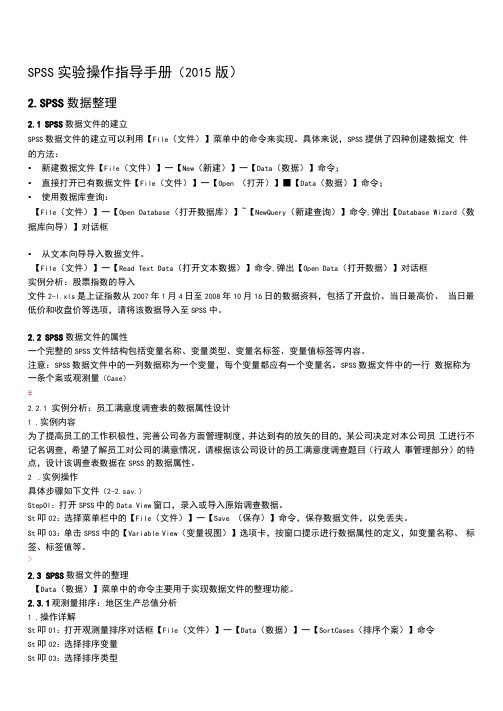
SPSS实验操作指导手册(2015版)2.SPSS数据整理2.1SPSS数据文件的建立SPSS数据文件的建立可以利用【File(文件)】菜单中的命令来实现。
具体来说,SPSS提供了四种创建数据文件的方法:•新建数据文件【File(文件)】一【New(新建)】一【Data(数据)】命令;•直接打开已有数据文件【File(文件)】一【Open (打开)】■【Data(数据)】命令;•使用数据库查询:【File(文件)】一【Open Database(打开数据库)】~【NewQuery(新建查询)】命令,弹出【Database Wizard(数据库向导)】对话框•从文本向导导入数据文件。
【File(文件)】一【Read Text Data(打开文本数据)】命令,弹出【Open Data(打开数据)】对话框实例分析:股票指数的导入文件2-l.xls是上证指数从2007年1月4日至2008年10月16日的数据资料,包括了开盘价、当日最高价、当日最低价和收盘价等选项,请将该数据导入至SPSS中。
2.2SPSS数据文件的属性一个完整的SPSS文件结构包括变量名称、变量类型、变量名标签、变量值标签等内容。
注意:SPSS数据文件中的一列数据称为一个变量,每个变量都应有一个变量名。
SPSS数据文件中的一行数据称为一条个案或观测量(Case)¥2.2.1实例分析:员工满意度调查表的数据属性设计1.实例内容为了提高员工的工作积极性,完善公司各方面管理制度,并达到有的放矢的目的,某公司决定对本公司员工进行不记名调查,希望了解员工对公司的满意情况。
请根据该公司设计的员工满意度调查题目(行政人事管理部分)的特点,设计该调查表数据在SPSS的数据属性。
2.实例操作具体步骤如下文件(2-2.sav.)StepOl:打开SPSS中的Data View窗口,录入或导入原始调查数据。
St叩02:选择菜单栏中的【File(文件)】一【Save (保存)】命令,保存数据文件,以免丢失。
SPSS实验指导书
SPSS实验指导书SPSS统计分析软件概述SPSS(Statistical Package for the Social Science)社会科学统计软件包;SPSS(Statistical Product and Service Solutions)统计产品与服务解决方案。
20世纪60年代末,美国斯坦福大学的三位研究生研制开发了最早的统计分析软件SPSS,并于1975年在芝加哥成立了研发和经营SPSS软件的SPSS公司。
随着微型计算机和操作系统的发展,SPSS公司相继推出了17个版本。
SPSS使用基础(安装和启动略)SPSS有两个基本窗口,分别是数据编辑窗口(Data Editor)和结果输出窗口(Viewer)。
数据编辑窗口(Data Editor)是SPSS的主程序窗口,在软件启动时自动打开,直到退出。
运行时只能打开一个数据编辑窗口,关闭该窗口意味着退出。
该窗口的主要功能:定义SPSS数据的结构、录入编辑和管理待分析的数据。
SPSS的所有统计分析功能都是针对该窗口中的数据的。
这些数据通常以SPSS数据文件的形式保存在计算机磁盘上,其文件扩展名为.sav。
数据编辑窗口由窗口主菜单、工具栏、数据编辑区、系统状态显示区组成。
1、窗口主菜单窗口主菜单将SPSS常用的数据编辑、加工和分析的功能列了出来。
2、工具栏将一些常用的功能以图形按钮的形式组织在工具栏,使操作更加快捷和方便。
3、数据编辑区显示和管理SPSS数据结构和数据内容的区域。
(数据视图和变量视图)4、系统状态显示区显示系统的当前运行状态。
SPSS结果输出窗口(Viewer)该窗口的主要功能是显示管理SPSS统计分析结果、报表及图形,允许同时创建或打开多个输出窗口。
SPSS统计分析的所有输出结果都显示在该窗口中。
输出结果通常以SPSS输出文件的形式保存在计算机的磁盘上,其文件扩展名为.spo。
SPSS的数据编辑窗口是专门负责输入和管理待分析数据的,而输出窗口则负责接收和管理统计分析的结果。
spss软件应用、统计学实验指导书
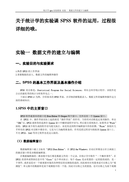
关于统计学的实验课SPSS软件的运用,过程很详细的哦。
实验一数据文件的建立与编辑一、实验目的与实验要求1.熟悉SPSS的工作界面2.掌握数据的录入、数据文件的编辑和操作二、SPSS的基本工作界面及基本操作介绍SPSS的全称是:Statistical Program for Social Sciences,即社会科学统计程序。
该软件是公认的最优秀的统计分析软件包之一。
下面以SPSS 14为例,介绍基本的SPSS界面,并详细讲解数据录入,数据文件的编辑和操作这方面的基础知识。
1.SPSS中的主要窗口SPSS软件最基本的窗口是Data Editor和Output两个窗口。
另外还有一个Syntax窗口。
在SPSS中,操作界面实际上起的就是“操作界面”的作用。
当你用对话框选定某项操作,单击“OK”后,SPSS就将你的选择在Syntax窗口中翻译成程序语句,然后提交系统执行。
如果单击“Paste”按钮,SPSS就不将生成的程序语句提交执行,而是传送到程序编辑窗中供你折腾。
“Paste”按钮在几乎所有的SPSS对话框中都存在,它是专门为编程准备的,作用是把过程语句粘贴到Syntax窗口上。
不光SPSS,SAS等其它软件也是这么做的。
(1)数据编辑窗口数据编辑窗口最上方标有“SPSS Data Editor”。
在SPSS for Windows 启动后屏幕显示在主画面上的激活窗口即是该数据编辑窗。
在数据编辑器的二维表格中每行都是数据文件的一个记录,在统计学中称作“一个概率事件”。
在SPSS的菜单或帮助信息中用“Cases”这个单词表示。
每个Cases是由变量的一定的值组成的,是一个事件,或者说是对一个被观察对象的各种特征的实测值组成的。
因此相对应变量来说可以称之为“观测值”。
单元格中的数据即是某个观测值中的一个值,因此可以称之为变量值,也可以称之为某个观测值,在Help信息中往往使用Case这个单词。
注意到页面下方有Data View和Variable View两个标签。
SPSS实验指导书

SPSS实验指导书三峡大学经济与管理学院2008年6月实验一SPSS基本介绍实验目的掌握什么是SPSS?该软件具有什么功能?熟悉SPSS菜单各项的含义,数据输入、存储以及数据运算与处理等。
实验内容1.什么是SPSS2.SPSS的菜单3.数据输入与保存4.数据编辑整理5.变量重新赋值6.数据的运算与新变量的生成7.数据的排序8.数据分组基本步骤当打开SPSS后,展现在我们面前的界面如下:菜单栏共有10个选项:1.File:文件管理菜单,有关文件的调入、存储、显示和打印等;2.Edit:编辑菜单,有关文本内容的选择、拷贝、剪贴、寻找和替换等; 3.View:显示菜单,有关状况栏、工具条、网格线是否显示,以及数据显示的字体类型、大小等设置;4.Data:数据管理菜单,有关数据变量定义、数据格式选定、观察对象的选择、排序、加权、数据文件的转换、连接、汇总等;5.Transform:数据转换处理菜单,有关数值的计算、重新赋值、缺失值替代等;6.Analyze:统计菜单,有关一系列统计方法的应用;7.Graphs:作图菜单,有关统计图的制作;8.Utilities:用户选项菜单,有关命令解释、字体选择、文件信息、定义输出标题、窗口设计等;实验报告自己草拟10名学生的序号、姓名、统计学成绩、每天学习时间特征资料。
要求:(1)添加性别数据特征;粘贴处(2)按统计学成绩由高到低排序;粘贴处(3)按统计学成绩数量标志进行等距分组。
粘贴处实验二SPSS统计绘图实验目的掌握条形图、线形图、散点图、直方图等常用统计图的绘制方法与技巧。
实验内容1.条形图1.绘制简单条图(单式条图)2.绘制复式条图3.绘制堆积条图(分段条图)定义统计图中数据的表达类型:条图反映了同一变量若干条记录的分组汇总条图反映了不同变量的汇总条图反映了个体观察值2.线形图单线形图(Simple)多线形图(Multiple)垂线形图(Drop-line)3.散点图简单散点图(Simple)——显示一对相关变量关系;重叠散点图(Overlay) ——显示多对相关变量关系;矩阵散点图(Matrix) ——显示多个相关变量关系;3维散点图(3-D) ——显示3个相关变量关系。
SPSS实验指导书

SPSS实验指导书目录上机1:描述统计 (2)一、上机目的 (2)二、上机要求 (2)三、上机演示内容与步骤 (2)四、上机1报告概要 (13)上机2:统计图的绘制 (13)一、上机目的 (13)二、上机演示内容与步骤 (13)三、上机2报告概要 (17)上机3:点估计与区间估计 (18)一、上机目的 (18)二、上机演示内容与步骤 (18)上机4:相关分析 (26)一、上机目的 (26)二、上机演示内容与步骤演示 (26)上机5:回归分析 (30)一、上机目标 (30)二、上机要求 (30)三、上机演示内容与步骤 (30)上机1:描述统计一、上机目的1.学会应用两种以上的方法完成描述统计学所学的统计量的计算程序;如列出数据的频数分布表;计算算术平均数、中位数、众数;计算全距、四分位差、标准差、方差等。
2.能够完成统计图的绘制(主要包括直方图、曲线图、饼形图、茎叶图);3.能够撰写出规范的描述统计分析报告。
二、上机要求1.前20分钟,主讲老师通过例题演示描述统计方法的应用;2.中间70分钟,学生仿照演示题,独立做一个练习题目;期间老师课堂巡视,随时解决学生提出的问题;3.后20分钟,每位同学将自己的计算结果,以Word形式,撰写成统计分析报告,老师给出是否合格的评价。
4.在完成练习题的时候,鼓励学生之间相互交流探讨;5.鼓励学生尝试发现软件的新功能。
三、上机演示内容与步骤下面给出的一个例题是来自SPSS软件自带的数据文件“Employee.data”,该文件包含某公司员工的工资、工龄、职业等变量,我们将利用此例题给出相关的描述统计说明,本例中,我们将以员工的当前工资为例,计算该公司员工当前工资的一些描述统计量,如均值、频数、方差等描述统计量的计算。
计算各项描述统计量值的程序使用步骤如下:步骤1:用SPSS打开已知的数据文件选择菜单“File—>Open—>Data”,在对话框中找到需要分析的数据文件“SPSS/Employee data”,然后选择“打开”。
spss软件实验指导书

SPSS统计分析软件实验指导书经济与管理学院工商管理系统计模拟实习课程组2011年2月目录1.实验一 SPSS的数据基本操作2.实验二描述性统计分析3.实验三均值比较4.实验四相关分析和回归分析5.实验五聚类分析和判别分析6.实验六因子分析和主成分分析《SPSS统计分析软件实验》一、课程实验课所占学时30学时二、实验适用专业经济管理类各专业三、实验的任务、性质和目的统计计算,尤其是多元统计计算往往是十分复杂的,因此需要借助统计软件。
本课程实验正是为了使学生系统地学习SPSS这一统计软件,培养学生根据实际问题建立SPSS数据文件、利用SPSS软件提供的各种统计功能进行统计分析,并结合一定专业知识对分析结果给出合理解释的能力,从而为学生以后从事统计分析工作打下基础。
四、实验方式与基本要求1.由授课教师讲清上机实验的基本要求和注意事项;2.由授课教师事先布置上机实验的内容,设计要求,操作步骤,并要求学生课前进行准备;3.学生集中在机房上机;4.要求学生每次完成所布置的任务,提交实验报告。
五、考核方式与评分办法1.实验报告(60%)2.上机检查(20%)3.考勤(20%)实验一SPSS基本操作一、实验目的1.熟悉SPSS的菜单和窗口界面,熟悉SPSS各种参数的设置;2.掌握SPSS的数据管理功能。
二、实验内容及步骤(一)数据的输入和保存1. SPSS界面当打开SPSS后,展现在我们面前的界面如下:请注意窗口顶部显示为“SPSS for Windows Data Editor”,表明现在所看到的是SPSS的数据管理窗口。
这是一个典型的Windows软件界面,有菜单栏、工具栏。
该界面和EXCEL极为相似,很多操作也与EXCEL类似,同学们可以自己试试。
2.定义变量选择菜单Data==>Define Variable。
系统弹出定义变量对话框如下:对话框最上方为变量名,现在显示为“VAR00001”,这是系统的默认变量名;往下是变量情况描述,可以看到系统默认该变量为数值型,长度为8,有两位小数位,尚无缺失值,显示对齐方式为右对齐;第三部分为四个设置更改按钮,分别可以设定变量类型、标签、缺失值和列显示格式;第四部分实际上是用来定义变量属于数值变量、有序分类变量还是无序分类变量,现在系统默认新变量为数值变量;最下方则依次是确定、取消和帮助按钮。
SPSS实验指导手册(定稿)

实验一 SPSS的数据管理[目的要求]熟悉SPSS的菜单和窗口界面及SPSS的数据管理功能。
[实验内容][实验步骤][实验结果]实验二描述性统计分析 [目的要求]利用SPSS进行描述性统计分析。
[实验内容][实验步骤]1、定义变量,建立数据文件并输入数据。
2、选择菜单“Analyze→Descriptive Statistics→Frequencies”,选择分析变量,要输出的统计量以及要绘制的统计图,即完成了频数分析。
3、在1的基础上,选择菜单“Analyze→Descriptive Statistics→Descriptives”,选择分析变量即完成了描述性分析。
4、在1的基础上,选择菜单“Analyze→Descriptive Statistics→Explore”,选择Dependent变量和Factor变量,要输出的统计量以及要绘制的统计图,即完成了探索分析。
5、在1的基础上,首先对频数变量的值进行加权处理,再选择菜单“Analyze→DescriptiveStatistics→Crosstabs”,选择分组变量和分析变量,然后选择卡方检验,定义列联表单元格中需要计算的指标,即完成了交叉列联表分析。
实验三均值检验[目的要求]利用SPSS进行单样本、两独立样本以及成对样本的均值检验。
[实验内容](一)描述统计(Means过程)某医师测得血红蛋白值(g%)如表3.1,试利用Means过程作基本的描述性统计分析。
实验步骤:1.建立数据文件。
定义4个变量:ID、Gender、Age和HB,分别表示编号、性别、年龄和血红蛋白值。
2. 选择菜单“Analyze→Compare Means→Means”,弹出“Means”对话框。
在对话框左侧的变量列表中,选择变量“血红蛋白值”进入“Dependent List”列表框,选择变量“性别”进入“Independent List”,单击“Next”按钮,选择变量“年龄”进入“Independent List”。
- 1、下载文档前请自行甄别文档内容的完整性,平台不提供额外的编辑、内容补充、找答案等附加服务。
- 2、"仅部分预览"的文档,不可在线预览部分如存在完整性等问题,可反馈申请退款(可完整预览的文档不适用该条件!)。
- 3、如文档侵犯您的权益,请联系客服反馈,我们会尽快为您处理(人工客服工作时间:9:00-18:30)。
(完整)SPSS实验指导手册(定稿)编辑整理:尊敬的读者朋友们:这里是精品文档编辑中心,本文档内容是由我和我的同事精心编辑整理后发布的,发布之前我们对文中内容进行仔细校对,但是难免会有疏漏的地方,但是任然希望((完整)SPSS实验指导手册(定稿))的内容能够给您的工作和学习带来便利。
同时也真诚的希望收到您的建议和反馈,这将是我们进步的源泉,前进的动力。
本文可编辑可修改,如果觉得对您有帮助请收藏以便随时查阅,最后祝您生活愉快业绩进步,以下为(完整)SPSS实验指导手册(定稿)的全部内容。
实验一 SPSS的数据管理[目的要求]熟悉SPSS的菜单和窗口界面及SPSS的数据管理功能.[实验内容][实验步骤][实验结果]实验二描述性统计分析[目的要求]利用SPSS进行描述性统计分析。
[实验内容][实验步骤]1、定义变量,建立数据文件并输入数据.2、选择菜单“Analyze→Descriptive Statistics→Frequencies”,选择分析变量,要输出的统计量以及要绘制的统计图,即完成了频数分析.3、在1的基础上,选择菜单“Analyze→Descriptive Statistics→Descriptives",选择分析变量即完成了描述性分析。
4、在1的基础上,选择菜单“Analyze→Descriptive Statistics→Explore",选择Dependent变量和Factor变量,要输出的统计量以及要绘制的统计图,即完成了探索分析.5、在1的基础上,首先对频数变量的值进行加权处理,再选择菜单“Analyze→DescriptiveStatistics→Crosstabs",选择分组变量和分析变量,然后选择卡方检验,定义列联表单元格中需要计算的指标,即完成了交叉列联表分析。
实验三均值检验[目的要求]利用SPSS进行单样本、两独立样本以及成对样本的均值检验。
[实验内容](一)描述统计(Means过程)某医师测得血红蛋白值(g%)如表3.1,试利用Means过程作基本的描述性统计分析。
3。
11.建立数据文件.定义4个变量:ID、Gender、Age和HB,分别表示编号、性别、年龄和血红蛋白值.2。
选择菜单“Analyze→Compare Means→Means”,弹出“Means"对话框.在对话框左侧的变量列表中,选择变量“血红蛋白值”进入“Dependent List”列表框,选择变量“性别”进入“Independent List”,单击“Next"按钮,选择变量“年龄”进入“Independent List"。
3.单击“Options”按钮,在弹出的“选择描述统计量”对话框中设置输出的描述统计量。
4.单击“OK”按钮,得到输出结果.(二)单样本T检验(One—Sample T Test过程)实验步骤:(三)双样本T检验(Independent—Samples T Test过程)实验步骤:(四)成对样本的均值检验实验四方差分析[目的要求]利用SPSS进行单因素方差分析、多因素方差分析和协方差分析.[实验内容](一)单因素方差分析(One—Way ANOVA过程)(二)多因素方差分析(Univariate过程)实验步骤:1.建立数据文件.定义变量名:编号、大肠杆菌数量、处理方法和排污口的变量名分别为x1、x2、x3和x4,之后输入原始数据。
2。
选择菜单“Analyze→ General Linear Model→ Univariate”,弹出“多因素方差分析”对话框。
在对话框左侧的变量列表中选择变量“大肠杆菌数量"进入“Dependent Variable”框,选择“排污口”和“处理方法”进入“Fixed Factor(s)”框。
3.选择建立多因素方差分析的模型.单击“Univariate"对话框中的“Model”按钮,弹出“Un ivariate: Model"对话框.选中“Full Factorial”单选纽即饱和模型。
4.设置多因素变量的各组差异比较。
单击“Contrasts”按钮,弹出“Univariate:Contrasts”对话框,在“Contrasts”下拉框中选择Simple;单击“Change”按钮可改变多因素变量的各组差异比较类型.5.设置以图形方式展现多因素之间是否存在交互作用。
单击“Plots”按钮,弹出“Univariate:Profile Plots”对话框。
选择变量“排污口"进入“Hor izontal Axis"编辑框,单击“ADD”进入“Plots"框后,选择变量“处理方法”进入“Horizontal Axis”编辑框,单击“ADD”进入“Plots"框。
6.设置均值多重比较类型。
单击“Post Hoc"按钮,弹出“Univariate:Post Hoc Multiple Comparisons for Observed Means”对话框。
将因素“排污口”选入“Post Hoc Test for”列表框,进行多重比较分析。
在“Equal Variances Assumed”复选框组中,选择LSD法进行方差齐时两两均值的比较。
7.设置输出到结果窗口的选项。
单击“Options"按钮,弹出“Univariate:Options”对话框,在“Display”复选框中选择Descriptive statistics和Homogeneity tests。
8.单击“OK”按钮,执行多因素方差分析,得到输出结果。
(三)协方差分析(Univariate过程)政府实施某个项目以改善部分年轻工人的生活状况。
项目实施后开始对年轻工人生活的改善情况进行调查,调查项目包括工人受教育程度、是否实施了该项目、实施项目前的工资(前工资)和实施项目后的工资(后工资)如下表所示.用实施项目后的工资来反映生活状况的改善,要求剔除实施项目前的工资差异,分析工人的受教育程度和该项目实施对工人收入的提高是否1.建立数据文件。
定义5个变量:x1、x2、x3、x4和x5,分别表示编号、前工资、后工资、受教育程度和项目实施。
注意:这5个变量都应是数值型的。
2.选择菜单“Analyze→General Linear Model→Univariate”,弹出“多因素方差分析”对话框。
3.选择进行协方差分析的变量。
在对话框左侧的变量列表中选择变量“后工资”进入“Dependent Variable”框;选择变量“受教育程度”和“项目实施”进入“Fixed Factor(s)"框;选择变量“前工资”进入“Covariate(s)”框.4.选择建立多因素方差分析的模型。
单击“Model”按钮,弹出“Univariate:Model”对话框,选择饱和模型。
5.其他设置与多因素方差分析类似,在此略。
6.单击“OK”按钮,执行协方差分析,得到输出结果。
实验五相关分析和回归分析[目的要求]利用SPSS进行简单相关分析、偏相关分析、距离分析、一元线性回归分析和多性元线回归。
[实验内容](一)两变量的相关分析(Bivariate过程)(二)偏相关分析(Partial 过程)(三)距离分析(Distances过程)(四)一元回归分析(Linear过程)(五)多元回归分析(Linear过程)实验六绘制统计图[目的要求]利用SPSS绘制各种统计图.[实验内容](一)直条图.实验步骤:1.建立数据文件。
原数据输入,DISEASE按冠状动脉机能不全=1、猝死=2、心绞痛=3、心肌梗塞=4输入,BP按正常=1、临界=2、异常=3输入。
2.选择菜单“Graphs→Bar”过程,弹出“Bar Chart”定义选项框。
在定义选项框的上方选择复式直条图“Clustered”。
3.单击“Define"钮,弹出“Define Clustered Bar: Summaries for Groups of Cases”对话框,在左侧的变量列表中选择变量rate,使之进入“Bars Represent”栏的“Other summary function”选项的“Variable”框,选择变量disease,使之进入“Category Axis"框,并选择变量bp进入“Define Clusters by”框.4.单击“Titles”钮,弹出“Titles"对话框,在“Title”栏内输入“血压状态与冠心病各临床型年龄标化发生率的关系”,单击“Continue”按钮返回“Define Clustered Chart: Summaries for Groups of Cases对话框。
5.单击“OK“按钮,得到输出结果。
(二)线图某地调查居民心理问题的存在现状,资料如下表所示,试绘制线图比较不同性别和年龄组的居民心理问题检出情况。
年龄分组心理问题检出率(%)男性女性15—25—35-45-55—65-75—10.5711。
579.5711。
7113.5115.0216.0019.7311.9815.5013.8512.9116.7721.04实验步骤:1.建立数据文件。
定义变量名:心理问题检出率为RATE,年龄分组为AGE,性别为SEX,AGE与SEX可定义为字符变量。
RATE按原数据输入,AGE按分组情况分别输入15—、25—、35—、45-、55-、65-、75—,SEX是男的输入M、女的输入F.2.选择菜单“Graphs→Line”,弹出Line Chart定义选项框,选择” Multiple“绘制多条线图。
3.单击“Define”按钮,弹出“Define Multiple Line: Summaries for Groups of Case s”对话框,在左侧的变量列表中选择变量rate,使之进入“Lines Represent"栏的“Other summary function”选项的“Variable"框,选择变量age,使之进入“Category Axis”框,选择变量sex,使之进入“Define Lines by”框.4.单击“Titles”按钮,弹出“Titles"对话框,在“Title”栏内输入“某地男女性年龄别心理问题检出率比较”,单击“Continue”按钮返回“Define Multiple Line: Summaries for Groups of Cases”对话框。
5.单击“OK"按钮,得到输出结果。
(三)区域图实验内容:在某城市抽样研究20—49岁已婚育龄妇女的避孕现状,频数分布资料参见下表,试绘制区域图。