行列式的计算外文文献及翻译
行列式的计算外文文献及翻译

1 The definition of determinant:n order determinant represented by the symbol nnn n nn a a a a a a a a a 212222111211n D =It represents the n!Algebra and items.These are all possible from different lines in different columns in the N element of the n nj j j a a a 2121 product.n nj j j a a a 2121symbols for )(21)1(n j j j τ-.When n j j j 21 iseven (odd) arrangement of the sign is positive (negative) .That is to sayn nn nj j j j j j j j j a a a 21212121)(n )1(D ∑-=τ.Here are∑nj j j 21 said the summation of all n order.Definition of determinant by inverse number given, should grasp the following four:(1) The total number of n order permutation is !n so the n order determinant expansion there are !n ;(2) Each item is taken from different lines, product of n elements in different columns;(3) The premise in subscript according to the natural number sequence, the parity of the inverse number each item in front of the sign depends on the column index consisting of the arrangement of the evidence, the other half, half of them take the negative; (4) A number is the value of determinant..Example 1: if the permutation inversions number n j j j 21 to I .How much is the inverse number and arrangement of 121j j j j n n -.Analysis:If the number of the original array.1j earlier than 1j large number of 1τ, a number of smaller than 1j number is 1)1(τ--n , and the number of new arrangement of 121j j j j n n -1j earlier than 1j large number of as 1)1(τ--n ; similarly, a number of the original arrangement set before 2j than 2j a large number of 2τ, a number of smaller than 2j number is2)2(τ--n , and the number of new arrangement of 2j earlier than 2j large number of as2)2(τ--n ; followed by analogy, a number of the original arrangement set before k j than k j large number of k τ, t he number of new arrangement in k j before the number greaterthan k j for ),,2,1()(n k k n k =--τ.Solution: a number of set the original permutation of k j than k j large number of k τ, a new arrangement ofk j earlier than k j large number of a number of),,2,1()(n k k n k =--τ. Because of I n =+++τττ 21 so Inverse numberarrangementof121j j j j n n - isI n n k n n n n nk k -=+++-+++-+-=--=-=∑2)1(211)(]01)2()1[(])[(τττττ2 basic theory2.1 Properties of n order determinantProperty 1: Transpose, determinant. That isnnn n n n a a a a a a a a a212222111211=nnn nn n a a a a a a a a a212221212111Property 2: a number multiplied by the determinant of a row is equal to the number is multipliedby this determinant. That is nnn n l l nnn n n l l n a a a a a a a a a k a a a ka ka ka a a a21ln 211121121ln 2111211= Nature 3: if a line is the two set of numbers and then the determinant equals two determinant and the determinant in addition to this, all with the original determinant of the correspondingline.nnn n n n nn n n n n nn n n n n n a a a c c c a a a a a a b b b a a a a a a c b c b c b a a a 21211121121211121121221111211+=+++ Nature 4: if the determinant of two lines of the same so determinant is zero. The so-called two lines of the same is corresponding elements of two lines of equal.Nature 5: if the determinant of the two line is proportional to the determinant is zero.02121ln21112112121ln 2111211==nnn n ini i l l nnn n n ini i l l na a a a a a a a a a a a k a a a a a a a a a a a aNature 6: the same row to another row determinant factor.Nature 7: to wrap column position in two lines of the determinant of No. 2.2 basic theory1 ⎩⎨⎧≠=+++0,0,2211ji D A a A a A a jn in j i j i Where ij A is a cofactor of element ij a . 2 Reduction theoremB CA D A DCB A 1--=3CA CB A =4B A AB =5 the nonzero matrix K left by a row to another row determinant is the new block determinant and the original equal2.3 results of several special determinant 1 triangular determinantnn nnn n a a a a a a a a a 221122211211000=(Triangular determinant )nn nnn n a a a a a a a a a221121222111000=(Lower triangular determinant )2 diagonal determinantnn nna a a a a a 221122110000=3 Symmetric and anti-symmetric determinantnnn n nn a a a a a a a a a D 212222111211=To meet the )2,1,2,1(n j n i a a ji ij ===, D is calledsymmetric determinant000331332312232111312 n n n n nn a a a a a a a a a a a a D =To meet the )2,1,(n j i a a ji ij =-=, D is calledskew-symmetric determinant. If the order of n is odd then 0=D 4 Vandermonde determinant∏≤<≤-----==ni j j i n n n n n nn n a a a a a a a a a a a a a a D 111312112232221321)(1111。
范德蒙行列式的相关应用外文翻译

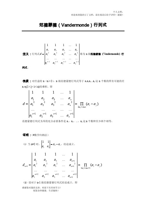
分类号:__________ 学校代码:11059学号:********** 毕业论文外文翻译材料学生姓名:学号: **********专业班级:数学一班指导教师:正文:外文资料译文附件:外文资料原文指导教师评语:签名:年月日范德蒙行列式的相关应用(一)范德蒙行列式在行列式计算中的应用 范德蒙行列式的标准规范形式是:1222212111112111()n n n i j n i j n n n nx x x D x x x x x x x x ≥>≥---==-∏根据范德蒙行列式的特点,将所给行列式包括一些非范德蒙行列式利用各种方法将其化为范德蒙行列式,然后利用范德蒙行列式的结果,把它计算出来。
常见的化法有以下几种:1.所给行列式各列(或各行)都是某元素的不同次幂,但其幂次数排列与范德蒙行列式不完全相同,需利用行列式的性质(如提取公因式,调换各行(或各列)的次序,拆项等)将行列式化为范德蒙行列式。
例1 计算222111222333n n n nD n n n =解 n D 中各行元素都分别是一个数自左至右按递升顺序排列,但不是从0变到n r -。
而是由1递升至n 。
如提取各行的公因数,则方幂次数便从0变到1n -.[]21212111111222!!(21)(31)(1)(32)(2)(1)13331n n n n D n n n n n n nn n ---==-------!(1)!(2)!2!1!n n n =--例2 计算1111(1)()(1)()1111n n n n n n a a a n a a a n D a a a n ---+----=--解 本项中行列式的排列规律与范德蒙行列式的排列规律正好相反,为使1n D +中各列元素的方幂次数自上而下递升排列,将第1n +列依次与上行交换直至第1行,第n 行依次与上行交换直至第2行第2行依次与上行交换直至第n 行,于是共经过(1)(1)(2)212n n n n n ++-+-+++=次行的交换得到1n +阶范德蒙行列式:[][](1)21111(1)211111(1)(1)()(1)()(1)(1)(2)()2(1)((1))!n n n n n n n nn n nk aa a n D a a a n a a a n a a a a a n a a a a n a n k ++---+=--=-----=--------------=∏ 若n D 的第i 行(列)由两个分行(列)所组成,其中任意相邻两行(列)均含相同分行(列);且n D 中含有由n 个分行(列)组成的范德蒙行列式,那么将n D 的第i 行(列)乘以-1加到第1i +行(列),消除一些分行(列)即可化成范德蒙行列式: 例3 计算1234222211223344232323231122334411111sin 1sin 1sin 1sin sin sin sin sin sin sin sin sin sin sin sin sin sin sin sin sin D +Φ+Φ+Φ+Φ=Φ+ΦΦ+ΦΦ+ΦΦ+ΦΦ+ΦΦ+ΦΦ+ΦΦ+Φ解 将D 的第一行乘以-1加到第二行得:123422221122334423232323112233441111sin sin sin sin sin sin sin sin sin sin sin sin sin sin sin sin sin sin sin sin ΦΦΦΦΦ+ΦΦ+ΦΦ+ΦΦ+ΦΦ+ΦΦ+ΦΦ+ΦΦ+Φ再将上述行列式的第2行乘以-1加到第3行,再在新行列式中的第3行乘以-1加到第4行得:12342222141234333412341111sin sin sin sin (sin sin )sin sin sin sin sin sin sin sin i j j i D ≤<≤ΦΦΦΦ==Φ-ΦΦΦΦΦΦΦΦΦ∏例4 计算211122222111111111nnnn nnx x x x x x D x x x ++++++=+++ (1)解 先加边,那么22111111222222222210001111111111111111111n n nn n n n nnnnnx x x x x x D x x x x x x x x x x x x ---+++=+++=+++ 再把第1行拆成两项之和,2211111122111120001111nnn n nnnnnnx x x x x x D x x x x x x =-11111112()(1)()()[2(1)]nnk j i k j j k ni j k nnnk j i i j k ni i x x x x x x x x x x x ≤<≤=≤<≤≤<≤===----=---∏∏∏∏∏∏2.加行加列法各行(或列)元素均为某一元素的不同方幂,但都缺少同一方幂的行列式,可用此方法: 例5 计算2221233312121113n n nnn nx x x D x x x x x x =解 作1n +阶行列式:122222121333312121111n nn nnnn n nz x x x z x x x D z x x x z x x x +==1()()ni j k i l k j nx z x x =≤<≤--∏∏由所作行列式可知z 的系数为D -,而由上式可知z 的系数为:211211(1)()()nn n j k i n j k li x x x x x x -=≥>≥--∑∏通过比较系数得:1211()()nn j k i n j k li D x x x x x x =≥>≥=-∑∏ 3.拉普拉斯展开法运用公式D =1122n n M A M A M A ++来计算行列式的值:例6 计算111111122122111000010010000100100001n n n n n n n n nnx x y y x x D y y x x y y ------=解 取第1,3,21n -行,第1,3,21n -列展开得: 11111111222211111111n n n n n n nn nnx x y y x x y y D x x y y ------==()()j i j i n j i lx x y y ≥>≥--∏4.乘积变换法 例7 设121(0,1,22)nk k k k k ni i s x x x x k n ==+++==-∑,计算行列式01112122n n n nn s s s s s s D s s s ---=解11121111222111nnn iii i nnn n iiii i i nnnn n n iii i i nxxxxx D xxx-=====--====∑∑∑∑∑∑∑∑211111221222222122111122111111()n n n nn n n n nnnnj i l i j nx x x x x x x x x x x x x xxx x x x x -----≤<≤==-∏例8 计算行列式000101011101()()()()()()()()()n n n n n n n n nnnn n n n a b a b a b a b a b a b D a b a b a b ++++++=+++解 在此行列式中,每一个元素都可以利用二项式定理展开,从而变成乘积的和。
行列式的计算方法文献综述
行列式的计算方法文献综述行列式是线性代数中的重要概念,广泛应用于各个科学领域的数学问题中。
在计算行列式的过程中,有多种方法可供选择,本综述将对其中几种主要的计算方法进行介绍和比较。
一、初等变换法:初等变换法是最早也是最基础的行列式计算方法之一、该方法通过对行列式进行一系列的初等行变换,将行列式转化为上(下)三角阵,然后通过对角线上元素的乘积得到行列式的值。
初等变换法的计算过程较为简单,易于操作。
然而,初等变换法需要进行多次的计算操作,当行列式的规模较大时,计算效率会较低。
二、按行(列)展开法:按行(列)展开法是另一种常用的行列式计算方法。
该方法通过选择行或列,将行列式展开为多个较小规模的子行列式,并使用递归的方法计算子行列式的值,最终将这些子行列式的值代入求和得到行列式的值。
按行(列)展开法可以用于计算任意规模的行列式,计算过程相对简单明了。
然而,按行(列)展开法需要进行多次的递归计算,这在计算较大规模的行列式时可能会导致计算时间过长。
三、特征值法:特征值法是一种较为高级的行列式计算方法。
该方法通过求解行列式与特征值之间的关系式,将行列式的计算转化为特征值的计算。
具体而言,首先求解特征值,然后根据特征值求解特征向量,最后代入特征向量计算行列式的值。
特征值法相对于初等变换法和按行(列)展开法而言,计算过程更为复杂,但其思想更加深入和抽象,适用于解决较为复杂的行列式计算问题。
四、Laplace定理:Laplace定理,也称为拉普拉斯展开定理,是另一种重要的行列式计算方法。
该定理通过选择行或列,将行列式展开为多个较小规模的子行列式,然后使用归纳的方法计算子行列式的值,最终将这些子行列式的值代入求和得到行列式的值。
Laplace定理可以看作是按行(列)展开法的一种推广和总结,通过较为规则的计算步骤,使得计算过程更加简洁和高效。
综上所述,行列式的计算方法有初等变换法、按行(列)展开法、特征值法和Laplace定理等。
行列式的计算方法和应用[开题报告]
![行列式的计算方法和应用[开题报告]](https://img.taocdn.com/s3/m/d3fdf277b90d6c85ed3ac636.png)
毕业论文开题报告信息与计算科学行列式的计算方法和应用一、选题的背景、意义(所选课题的历史背景、国内外研究现状和发展趋势)1.选题的背景行列式理论产生于十七世纪末,到十九世纪末,它的理论体系已基本形成了。
1693年,德国数学家莱布尼茨(Leibnie,1646—1716)解方程组时将系数分离出来用以表示未知量,得到行列式原始概念。
当时,莱布尼兹并没有正式提出行列式这一术语。
1729年,英国数学家马克劳林(Maclaurin,1698—1746)以行列式为工具解含有2、3、4个末知量的线性方程组。
在1748年发表的马克劳林遗作中,给出了比菜布尼兹更明确的行列式概念。
1750年,瑞士数学家克拉默(Gramer,1704—1752)更完整地叙述了行列式的展开法则并将它用于解线性方程组。
即产生了克拉默法则。
1772年。
法国数学家范德蒙(Vandermonde,1735—1796)专门对行列式作了理论上的研究,建立了行列式展开法则,用子式和代数余子式表示一个行列式。
1172年,法国数学家拉普拉斯(Laplace。
1749梷1827)推广了范德蒙展开行列式的方法。
得到我们熟知的拉普拉斯展开定理。
1813一1815年,法国数学家柯西(Cauchy,1789—1857,对行列式做了系统的代数处理,对行列式中的元素加上双下标排成有序的行和列,使行列式的记法成为今天的形式。
英国数学家凯菜(Cayley,于1841年对数字方阵两边加上两条竖线。
柯西证明了行列式乘法定理。
1841年,德国数学家雅可比(jacobi)发表的《论行列式的形成与性质》一文,总结了行列式的发展。
同年,他还发表了关于函数行列式的研究文章,给出函数行列式求导公式及乘积定理。
至19世纪末,有关行列的研究成果仍在式不断公开发表,但行列式的基本理论体系已经形成。
行列式的概念最初是伴随着方程组的求解而发展起来的。
行列式的应用早已超出了代数的范围,成为解析几何、数学分析、微分方程、概率统计等数学分支的基本工具,因此对许多人来说,掌握行列式的计算是重要的。
数学 外文翻译 外文文献 英文文献 矩阵
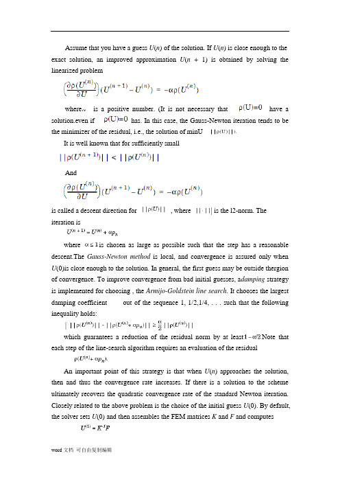
Assume that you have a guess U(n) of the solution. If U(n) is close enough to the exact solution, an improved approximation U(n + 1) is obtained by solving the linearized problemwhere have asolution.has. In this case, the Gauss-Newton iteration tends to be the minimizer of the residual, i.e., the solution of minUIt is well known that for sufficiently smallAndis called a descent direction for , where | is the l2-norm. The iteration iswhere is chosen as large as possible such that the step has a reasonable descent.The Gauss-Newton method is local, and convergence is assured only when U(0)is close enough to the solution. In general, the first guess may be outside thergion of convergence. To improve convergence from bad initial guesses, a damping strategy is implemented for choosing , the Armijo-Goldstein line search. It chooses the largestinequality holds:|which guarantees a reduction of the residual norm by at least Note that each step of the line-search algorithm requires an evaluation of the residualAn important point of this strategy is that when U(n) approaches the solution, then and thus the convergence rate increases. If there is a solution to the scheme ultimately recovers the quadratic convergence rate of the standard Newton iteration. Closely related to the above problem is the choice of the initial guess U(0). By default, the solver sets U(0) and then assembles the FEM matrices K and F and computesThe damped Gauss-Newton iteration is then started with U(1), which should be a better guess than U(0). If the boundary conditions do not depend on the solution u, then U(1) satisfies them even if U(0) does not. Furthermore, if the equation is linear, then U(1) is the exact FEM solution and the solver does not enter the Gauss-Newton loop.There are situations where U(0) = 0 makes no sense or convergence is impossible.In some situations you may already have a good approximation and the nonlinear solver can be started with it, avoiding the slow convergence regime.This idea is used in the adaptive mesh generator. It computes a solution on a mesh, evaluates the error, and may refine certain triangles. The interpolant of is a very good starting guess for the solution on the refined mesh.In general the exact Jacobianis not available. Approximation of Jn by finite differences in the following way is expensive but feasible. The ith column of Jn can be approximated bywhich implies the assembling of the FEM matrices for the triangles containing grid point i. A very simple approximation to Jn, which gives a fixed point iteration, is also possible as follows. Essentially, for a given U(n), compute the FEM matrices K and F and setNonlinear EquationsThis is equivalent to approximating the Jacobian with the stiffness matrix. Indeed, since putting Jn = K yields In many cases the convergence rate is slow, but the cost of each iteration is cheap.The nonlinear solver implemented in the PDE Toolbox also provides for a compromise between the two extremes. To compute the derivative of the mapping , proceed as follows. The a term has been omitted for clarity, but appears again in the final result below.The first integral term is nothing more than Ki,j.The second term is “lumped,” i.e., replaced by a diagonal matrix that contains the row j j = 1, the second term is approximated bywhich is the ith component of K(c')U, where K(c') is the stiffness matrixassociated with the coefficient rather than c. The same reasoning can beapplied to the derivative of the mapping . Finally note that thederivative of the mapping is exactlywhich is the mass matrix associated with the coefficient . Thus the Jacobian ofU) is approximated bywhere the differentiation is with respect to u. K and M designate stiffness and mass matrices and their indices designate the coefficients with respect to which they are assembled. At each Gauss-Newton iteration, the nonlinear solver assembles the matrices corresponding to the equationsand then produces the approximate Jacobian. The differentiations of the coefficients are done numerically.In the general setting of elliptic systems, the boundary conditions are appended to the stiffness matrix to form the full linear system: where the coefficients of and may depend on the solution . The “lumped”approach approximates the derivative mapping of the residual by The nonlinearities of the boundary conditions and the dependencies of the coefficients on the derivatives of are not properly linearized by this scheme. When such nonlinearities are strong, the scheme reduces to the fix-pointiter ation and may converge slowly or not at all. When the boundary condition sare linear, they do not affect the convergence properties of the iteration schemes. In the Neumann case they are invisible (H is an empty matrix) and in the Dirichlet case they merely state that the residual is zero on the corresponding boundary points.Adaptive Mesh RefinementThe toolbox has a function for global, uniform mesh refinement. It divides each triangle into four similar triangles by creating new corners at the midsides, adjusting for curved boundaries. You can assess the accuracy of the numerical solution by comparing results from a sequence of successively refined meshes.If the solution is smooth enough, more accurate results may be obtained by extra polation. The solutions of the toolbox equation often have geometric features like localized strong gradients. An example of engineering importance in elasticity is the stress concentration occurring at reentrant corners such as the MATLAB favorite, the L-shaped membrane. Then it is more economical to refine the mesh selectively, i.e., only where it is needed. When the selection is based ones timates of errors in the computed solutions, a posteriori estimates, we speak of adaptive mesh refinement. Seeadapt mesh for an example of the computational savings where global refinement needs more than 6000elements to compete with an adaptively refined mesh of 500 elements.The adaptive refinement generates a sequence of solutions on successively finer meshes, at each stage selecting and refining those elements that are judged to contribute most to the error. The process is terminated when the maximum number of elements is exceeded or when each triangle contributes less than a preset tolerance. You need to provide an initial mesh, and choose selection and termination criteria parameters. The initial mesh can be produced by the init mesh function. The three components of the algorithm are the error indicator function, which computes an estimate of the element error contribution, the mesh refiner, which selects and subdivides elements, and the termination criteria.The Error Indicator FunctionThe adaption is a feedback process. As such, it is easily applied to a lar gerrange of problems than those for which its design was tailored. You wantes timates, selection criteria, etc., to be optimal in the sense of giving the mostaccurate solution at fixed cost or lowest computational effort for a given accuracy. Such results have been proved only for model problems, butgenerally, the equid is tribution heuristic has been found near optimal. Element sizes should be chosen such that each element contributes the same to the error. The theory of adaptive schemes makes use of a priori bounds forsolutions in terms of the source function f. For none lli ptic problems such abound may not exist, while the refinement scheme is still well defined and has been found to work well.The error indicator function used in the toolbox is an element-wise estimate of the contribution, based on the work of C. Johnson et al. For Poisson'sequation –f -solution uh holds in the L2-normwhere h = h(x) is the local mesh size, andThe braced quantity is the jump in normal derivative of v hr is theEi, the set of all interior edges of thetrain gulation. This bound is turned into an element-wise error indicator function E(K) for element K by summing the contributions from its edges. The final form for the toolbox equation Becomeswhere n is the unit normal of edge and the braced term is the jump in flux across the element edge. The L2 norm is computed over the element K. This error indicator is computed by the pdejmps function.The Mesh RefinerThe PDE Toolbox is geared to elliptic problems. For reasons of accuracy and ill-conditioning, they require the elements not to deviate too much from beingequilateral. Thus, even at essentially one-dimensional solution features, such as boundary layers, the refinement technique must guarantee reasonably shaped triangles.When an element is refined, new nodes appear on its mid sides, and if the neighbor triangle is not refined in a similar way, it is said to have hanging nodes. The final triangulation must have no hanging nodes, and they are removed by splitting neighbor triangles. To avoid further deterioration oftriangle quality in successive generations, the “longest edge bisection” scheme Rosenberg-Stenger [8] is used, in which the longest side of a triangle is always split, whenever any of the sides have hanging nodes. This guarantees that no angle is ever smaller than half the smallest angle of the original triangulation. Two selection criteria can be used. One, pdead worst, refines all elements with value of the error indicator larger than half the worst of any element. The other, pdeadgsc, refines all elements with an indicator value exceeding a user-defined dimensionless tolerance. The comparison with the tolerance is properly scaled with respect to domain and solution size, etc.The Termination CriteriaFor smooth solutions, error equi distribution can be achieved by the pde adgsc selection if the maximum number of elements is large enough. The pdead worst adaption only terminates when the maximum number of elements has been exceeded. This mode is natural when the solution exhibits singularities. The error indicator of the elements next to the singularity may never vanish, regardless of element size.外文翻译假定估计值,如果是最接近的准确的求解,通过解决线性问题得到更精确的值当为正数时,( 有一个解,即使也有一个解都是不需要的。
LINEAR ALGEBRA 线性代数 课文 翻译

4 LINEAR ALGEBRA 线性代数“Linear algebra” is the study of linear sets of equations and their transformation properties. 线性代数是研究方程的线性几何以及他们的变换性质的Linear algebra allows the analysis of rotations in space, least squares fitting, solution of coupled differential equations, determination of a circle passing through three given points, as well as many other problems in mathematics, physics, and engineering.线性代数也研究空间旋转的分析,最小二乘拟合,耦合微分方程的解,确立通过三个已知点的一个圆以及在数学、物理和机械工程上的其他问题The matrix and determinant are extremely useful tools of linear algebra.矩阵和行列式是线性代数极为有用的工具One central problem of linear algebra is the solution of the matrix equation Ax = b for x. 线性代数的一个中心问题是矩阵方程Ax=b关于x的解While this can, in theory, be solved using a matrix inverse x = A−1b,other techniques such as Gaussian elimination are numerically more robust.理论上,他们可以用矩阵的逆x=A-1b求解,其他的做法例如高斯消去法在数值上更鲁棒。
范德蒙德行列式的证明
...
an
2 1
(ai a j )
1 jin1
... ...
...
a n2结论成立,即
感谢您对我的支持,欢迎下次再来学习! 祝您身体健康,生活愉快!
个人文档: 欢迎来到我的豆丁文档,请在阅读后给予评价!谢谢!
1
1
1
...
1
0 dn 0
... 0
a2 a1 a22 a1a2
范德蒙德行列式为零的充分必要条件是 a1,a2,...,an 这 n 个数种至少两个相等。
·证明:(#数学归纳法)
11
(i)当 n=2 时,
a1
a2 a2 a1 ,结论成立。
1 1 1 ... 1
a1 dn1 a12
... a1n2
a2 a22
... a2n2
a3 a32
... a3n2
... an1
个人文档: 欢迎来到我的豆丁文档,请在阅读后给予评价!谢谢!
范德蒙德(Vandermonde)行列式
1
a1 ·定义:行列式 d a12
... a1n1
列式。
1
a2 a22 ... a2 n 1
1
a3 a32 ... a3n1
... 1
... an ... an2 称为 n 级范德蒙德(Vandermonde)行 ... ... ... ann1
a n2 2
a n2 3
...
(a2 a1)(a3 a1)...(an a1) (ai a j ) 2 jin
1
an ... a n2
n
(ai a j ).......................................................|| 1 jin
行列式的计算 毕业论文

行列式的计算摘要: 行列式是研究许多学科的重要工具,因此行列式的计算是大家共同关注的问题.本文介绍了几种特殊而且行之有效的行列式的计算方法.关键词: 范德蒙行列式; 降阶法; 升阶法; 递推法; 数学归纳法; 代数余子式的计算; 拉普拉斯定理展开符号说明: i r 表示第 i 行j c 表示第j 列ij M 表示行列式元素ij a 的余子式 ij A 表示行列式元素ij a 的代数余子式i j kr r + 表示第 i 行的k 倍加到第j 行 i j kc c + 表示第 i 列的k 倍加到第j 列The Calculation of the DeterminantMA Zhi-e(College of Mathematics and Statistics, Northwest Normal University,Lanzhou 730070, Gansu, China)Abstract: The determinant is an important tool to study many disciplines, so the calculation of thedeterminant is a commonly concerned problem. Several particular and effective methods of calculating the determinant are introduced in this paper.Key words: Vandermonde determinant; reducing order method; ascending order method; recursive methods;mathematical induction; calculation of algebraic complement; method of Laplace expansion;引言使用行列式按行(列)展开,可以将行列式写成低一阶的行列式的代数和,从而将行列式降一阶.但是,由于展开式是n 项代数和,因此计算量任很大,可以考虑一些减少计算量的方法,并且选择最佳计算方法.行列式是研究许多学科的重要工具,因此行列式的计算是大家共同关注的问题.课本中只介绍了几种计算方法,本文主要介绍几种特殊而且行之有效的行列式的计算方法,具有针对性.一、化行列式为三角行列式使用行列式的性质将行列式化为三角行列式 ㈠ 箭形行列式例1.1 计算行列式11111201030100n D n= 解 1212,3,111110200030000j nj c c jn j njD n=+-=-=∑ 21!(1)nj n j==-∑ ㈡ 可化为箭形的行列式例1.2 计算n 阶行列式()123123123123,1,2,n nn n i i nx a a a a x a a D a a x a x a i n a a a x =≠=解 ()112311222,1133110000,2,in r r n i ni i n n x a a a a x x a D a x x a x a i n a x x a -+=--=--≠=--箭形行列式()()31211223311100=,2,10101001n n nni i i i i a a x a x a x a x a x a x a x a i n =------≠=--∏()()132122332,110100=,2,001001j nk n k k k n nnc c j niii i i x a a a x a x a x a x a x a x a i n =+==+-----≠=∑∏()111nnk i i k i k k x x a x a ==⎛⎫=+- ⎪-⎝⎭∑∏㈢ 行(列)和相等的行列式例1.3 计算n 阶行列式n x aa axa D a ax=解 ()()()()12,1111111j c cn j nx n a a a aa x n a xa x a D x n a x n a axax+=+-+-==+-⎡⎤⎣⎦+-()12,1010i r r i naa x a a x n a x a-+=-=+-⎡⎤⎣⎦-()()()11n x n a x a -=+--⎡⎤⎣⎦㈣ 相邻行(列)元素差1的行列式 以数字1,2n 为(大部分)元素,且相邻两行(列)元素相差1的n 阶行列式可如下计算:自第一行(列)开始,前行(列)减去后行(列),或自第n 行(列)开始,后行(列)减去前行(列),即可出现大量元素为1或1-的行列式.例1.4.1 计算n 阶行列式,=n ij ij D a a i j =-其中 解 由=ij a i j -得11,2,101221111111013211111214311111=2340111111123101231i i r r n i n n n n n n n D n n n n n n n nn+-+=-------------=-------------12,3,10000120001220012220123241jc cj nn n n nn +=------=--------()()12121n n n --=--例1.4.2 计算n 阶行列式1231234134512=11321221n n n n D n n n n nn n ------解 1,1,2123111*********111111111i ir r n i n n n n n n D n n--+=----=--()12,3,1231201111011110111101111j c cj nn n n n n n n n+=+---=-- ()11111111111211111111c n n n n n nn ---+=--按展开()12,3,1111111111211111111j c c j nn n n n n n+=-----+=---()12,3,1100100121001000jc cj nn n n n n n +=-----+=---()()()()()121221112n n n n n n n ----+=--()()112112n n n n n --+=-二、利用范德蒙行列式结果计算当行列式各行(列)都是某元素的不同次幂的形式,使用行列式的性质将行列式整理成范德蒙行列式.例2 计算行列式12222122221212111n n n n n n n nnnn x x x x x x D x x x x x x ---=解 考虑1n +阶范德蒙行列式()()()()()12222122221212122222121212222121111121211111111n n n n n n n nnnn n n n i j j i nn n n n n n n n n n nnnn n n x x x x x x D x x x x x x x x x x x x x x f x x x x x x x x x x x x x x x x x x x x x ---≤<≤--------+===----∏()1,1n n n n D f x x -+显然,就是辅助行列式中元素的余子式M ,即 ()1,1,1,1==1.n n n n n n n n n D +++++-=-M A A()()()1,1121n n n n ijj i nf x x x x x x x -+≤<≤=-++-∏而由的表达式知,的系数为A()()121n n ijj i nD x x x x x ≤<≤∴=++-∏三、降阶法使用行列式的性质将行列式的某行(列)化为只有一个非零元素,然后按这一行(列)展开,这样就可以将行列式降一阶,每展开一次,行列式的次数可以降低一阶,如此继续进行直到将行列式降到二阶行列式并求其值.这种方法对阶数不高的数字行列式比较适用.例3 计算n 阶行列式0000000000000000n x y x y x D y x y yx=解 ()110000001000000n c n xy y xx y D xy y xxy+=+-按展开()()111nn n n n n x y x y +=--=+-四、升阶法升阶法(也称加边法或镶边法),是在原行列式的基础上增加一行一列(即升一阶)且保持原行列式不变的情况下计算行列式的一种方法.可用升阶法计算的行列式一般应满足各行列含有共同元素的特点,且化简后常变成箭形行列式.例4.1 计算n 阶行列式()11212212120n n n n n na b a a a a b a D b b b a a a b ++=≠+解 1121211211222,3,212111101000=100010r r inn n n n i nn nnn n a a a a a a a b a a b D a a b a b a a a b b -+=+++-=+-+-加边1112111,2211000000000j jnjn j jc c b j nnn a a a a b b b b +=+=++=∑1211n jn j j a b b b b =⎛⎫=+ ⎪ ⎪⎝⎭∑例4.2 计算n 阶行列式2112122122212111nn nn n n n x x x x x x x x x x D x x x x x ++=+解 12211212212221211010101n n n nn n n n x x x x x x x x D x x x x x x x x x x ++=++加边111212,3,12110001001i inx r r i n nx x x x x x --+=+-=-- 1121212,3,11010001001j jni n i xc c j n x x x x -=+=++=∑211ni i x ==+∑五、递推法使用行列式的性质,将所求的n 阶行列式n D 用同样形式的1n -阶行列式1n D -表示出来,建立n D 与1n D -之间的递推关系,有时还可以将n D 用同样形式的比1n -阶更低阶的行列式表示,建立他们之间的递推关系,从而找到递推公式,最终求出n 阶行列式的值.例5.1 证明112211111nn i n i i nn n xxxD a x xa a a a a -=----==--∑证明 ()11111111n n n nn n x D xD a xD a x+----=+-=+-按c 展开()121n n n n n n D xD a x xD a a ---∴=+=++ 221n n n x D a x a --=++ 32321n n nn x D a x a x a ---=+++ =12121n n n n a x a x a x a ---=++++例5.2 计算n 阶行列式000n a aa b aa Db b a b b b= 解 n D n 将中第列元素表示成两数之和,然后拆成两个行列式相加,即()000000n a a a b a a b b a D b b ba a +++=+- 00000000a aa a ab aa b a b b a b b b b bab b ba=+- ()1n -将上式等号右边第一个行列式从第二行起,每一行的倍加到上一行,将第二个行列式按第列展开,得,1000000n n b a b a D aD b bbba---=--n 将上式等号右边第一个行列式按第列展开,得()11n n n D a b aD --=-- … ①a b 由字母与的对称性显然有()11n n n D b a bD --=-- … ②联立①②得,()()1111n n n n n n D aD a b D bD b a ----⎧⎫+=-⎪⎪⎨⎬+=-⎪⎪⎩⎭()()123321n n n n n n a b ab a a b ab b -----≠=-+++当时,可解得D ,()()111n n n a b n a -==--当时,易算出D六、数学归纳法当已知一个n 阶行列式的结果,要证明其等式对于任意的自然数都成立,常使用数学归纳法证明.如果未知n 阶行列式的结果,也可以先计算当1,2,3n =时的行列式值,推导出n 阶行列式的结果,然后使用数学归纳法证明结论的正确性.这种方法通常用在证明n 阶行列式的等于某个值的题目中.例6 证明1212111111111111111111111nn n i i n na a D a a a a a a =-++⎛⎫==+ ⎪⎝⎭++∑ 证明 1111111,.n n D a a a ⎛⎫==+=+ ⎪⎝⎭当时,所以结论成立12111kk k i in k D a a a a =⎛⎫==+ ⎪⎝⎭∑假设时结论成立,即 11k n k D +=+那么当时,将按最后一列拆开,有1122111110111111101111+11101111111111111k kkk a a a a D a a a ++++++=++121121000000=00011111k k k k k k a a a D a a a a D a +++=+12121111kk k k i i a a a a a a a a +=⎛⎫=++ ⎪⎝⎭∑1121111k k i i a a a a ++=⎛⎫=+ ⎪⎝⎭∑ 1n k ∴=+当时,结论亦成立.综上可知, 1212111111111111111111111nn n i i n na a D a a a a a a =-++⎛⎫==+ ⎪⎝⎭++∑.七、代数余子式的计算n ij n D a 设阶行列式=,则有结论1,0,nn ik jk k D i j a A i j ==⎧⎫=⎨⎬≠⎩⎭∑ 或1,0,nn ki kj k D i j a A i j==⎧⎫=⎨⎬≠⎩⎭∑ 利用上述表达式有时可以简化代数余子式的有关计算问题.例7 设n 阶行列式1231201030100n nD n=,求第一行各元素的代数余子式之和11121.n A A A +++解 显然第一行各元素的代数余子式之和可以表示成1112111111201030100n A A A n+++= 1212,3,21111102001!10030000j nj n c c jj nj jn j n=-+==-⎛⎫==- ⎪⎝⎭∑∑八、利用拉普拉斯展开定理计算拉普拉斯定理是行列式按一行或一列展开定理的推广.为了灵活应用拉普拉斯展开定理,必须正确理解其含义.该定理是说在n 阶行列式n D 中任意选定k 个行(列)(1,k n <<且这k 个行(列)不一定相连),位于这k 行(列)中所有k 阶子式i M (共k n C 个)与其相应的代数余子式i A 的乘积之和等于原行列式,即1knc n i i i D M A ==∑需要提醒的是i A 是i M 的代数余子式,计算i A 时不要遗漏其符号,即()111k ki i j j i i A N ++++=-11k k i i i i i j j M N M 其中,和,是所在行和列的序号,是的余子式.在利用拉普拉斯定理进行计算时,为使计算简便,一般选含零多的k 个行(列)展开. 例8 利用拉普拉斯定理计算2n 阶行列式22111324213n nn n n D nn n n +-+=+++解 2n D n n 因为的第1和2两行中不为0的2阶子式只有一个,因此按第1和2行展开,得()1212211213113242n nn n n n n D n n nn +++-++=-+++()()()()()21221222222n nn n D D D ---=-=-==-=-九、一题多解例9 计算n 阶行列式123123123123nn n n n a b a a a a a b a a D a a a ba a a a a b++=++解法1 n D 显然是一个各行和相同的行列式,故将各列都加到第一列上. 然后提取第一个公因子,可得,2323231231111nn nn i n i n a a a a b a a D b a a a ba a a a b=+⎛⎫=++ ⎪⎝⎭+∑12,3110001100100i i na c c i ni i b b a bb-+==⎛⎫=+ ⎪⎝⎭∑ 11nn i i bb a -=⎛⎫=+ ⎪⎝⎭∑解法2 11232,300000in r r n i na b a a a b b D b b bb-+=+-=--箭形12312,3000000i nin i c c i nb a a a a b b b=+=+=∑11nn i i bb a -=⎛⎫=+ ⎪⎝⎭∑解法3 n D 用加边法构造以下与相等的n+1阶行列式1121212122,3,121101000100010inn n r r n n i nn a a a a a a a b a a b D a a ba b a a a bb-+=+-=+=-+- 0n b D=若=0,显然b ≠不妨设0,112112,3110000000j nin i c c bn j na a a ab b D b b=+=+=∑111n ni i b a b =⎛⎫=+ ⎪⎝⎭∑11nn i i bb a -=⎛⎫=+ ⎪⎝⎭∑解法4 12312312312300n n n n n a b a a a a a b a a D a a a ba a a a a b++++=+++12312312312312312312312300n n n na b a a a a b a a a a b a a a a b a a a a ba a a ab a a a a a a a b++++=+++ n n 将上式等号右边的第一个行列式的各行都减去第行,将第二个行列式按第列展开,得11112300000000n n n n n nbb D b bD b a bD a a a a ---=+=+ ()1212n n n n n b a b b a bD ----=++11212n n n n n b a b a b D ----=++=()11121n n n n b a a a b D ---=++++ ()()11121n n n n b a a a b a b ---=+++++11nn i i bb a -=⎛⎫=+ ⎪⎝⎭∑参考文献【1】徐仲.线性代数典型题分析解集.2版.西北工业大学出版社,1997【2】赵慧斌,高旅瑞.线性代数专题分析与解题指导.北京大学出版社,2007,8【3】张天德,蒋晓芸.线性代数习题精选精解.山东科学技术出版社, 2009,12【4】上海交通大学数学系编. 线性代数习题与精解.2版. 上海交通大学出版社, 2004,6【5】刘书田,王中良编. 线性代数学习辅导与解题方法.高等教育出版社, 2003,7【6】徐仲,陆全等.高等代数考研教案. 2版.西北工业大学出版社, 2009,6【7】北京大学数学系几何与代数教研室前代数小组编.高等代数.第3版.高等教育出版社, 2003,2 【8】张禾瑞.高等代数同步辅导及习题全解.第5版.中国矿业大学出版社, 2009,2。
行列式的计算外文文献及翻译

1 行列式的定义:n 阶行列式用符号nnn n nna a a a a a a a a 212222111211n D =表示,它代表n !项的代数和,这些项是一切可能的取自于n D 中不同行不同列的n 个元素的乘积n nj j j a a a 2121,项n nj j j a a a 2121的符号为)(21)1(n j j j τ-,即当n j j j 21为偶(奇)排列时该项的符号为正(负),也就是说n nn nj j j j j j j j j a a a 21212121)(n )1(D ∑-=τ这里∑nj j j 21表示对所有n阶排列求和。
对于用逆序数给出的行列式的定义,应抓住如下四条:(1)n 阶排列的总数是!n 个,故n 阶行列式的展开式中共有!n 项; (2)每项是取自不同行,不同列的n 个元素的乘积;(3)在行下标按自然数顺序排列的前提下,每项前面的正负号取决于列下标组成的排列的逆序数的奇偶性,其中一半取证号另一半取负号;(4)行列式的值是一个数。
例1:如果排列n j j j 21的逆序数为I ,求排列121j j j j n n -的逆序数。
分析:如果设原排列中1j 前比1j 大的数的个数为1τ,则比1j 小的数的个数为1)1(τ--n ,于是新排列121j j j j n n -中1j 前比1j 大的数的个数为1)1(τ--n ;同理,设原排列中2j 前比2j 大的数的个数为2τ,则比2j 小的数的个数为2)2(τ--n ,于是新排列中2j 前比2j 大的数的个数为2)2(τ--n ;依次类推,设原排列中k j 前比k j 大的数的个数为k τ,则新排列中k j 前比k j 大的数的个数为),,2,1()(n k k n k =--τ。
解:设原排列中k j 前比k j 大的数的个数为k τ,则新排列中k j 前比k j 大的数的个数为),,2,1()(n k k n k =--τ。
行列式的计算与应用文献综述

文献综述
——行列式的一些计算方法一、本课题的背景和研究意义
背景:行列式起源于解二、三元线性方程组,然而它的应用早已超过代数的范围、成为研究数学领域各分支的基本工具。
本文主要对行列式的计算方法进行总结归纳,对行列式的应用做一定范围的探讨。
从行列式的的定义和性质入手,以具体实例为依据,对行列式的各种计算方法进行总结、归纳和比较。
研究意义:行列式经常被用于科学和工程计算中,如涉及到的电子工程、控制论、数学物理方程及数学研究等,都离不开行列式.其中最基本的就是行列式的计算,它是学习高等代数的基石,它是求解线性方程组、求逆矩阵及求矩阵特征值的基础。
但行列式的计算方法很多,综合性较强在行列式计算中需要我们多观察总结,便于我们能熟练的计算行列式的值。
目前我常用的计算行列式的方法有化三角形法、降阶法、数学归纳法。
同时我们还总结了几种尚未被大家广泛使用的方法
二、本课题国内外研究现状与发展趋势
行列式的计算一直是代数研究的一个重要课题,国内外学者专家已经总结了很多常用的技巧及方法,研究成果颇为丰硕。
对不同行列式,要针对其特征,选取适当的方法求解。
总结出来的计算方法主要有:定义法、化三角形法、拆行(列)法、降阶法、
升阶法(加边法)等等。
参考文献:
[1]北京大学数学系几何与代数教研室编. 高等代数.北京:高等教育出版社,2003.03第三版.
[2]张禾瑞、郝炳新编.高等代数. 北京:高等教育出版社,1983.07第三版
[3].同济大学数学系编: 工程数学.线性代数. 北京:高等教育出版社,2007.05第五版
[4] 方文波主编.线性代数及其应用.北京:高等教育出版社,2011.02。
行列式的计算毕业论文--中英文对照
X X 大学行列式的计算学生:学号:班级:专业:系别:指导教师:行列式的计算摘要:行列式是高等代数研究中的一个重要工具.本文从行列式的计算出发,通过例题,介绍行列式计算中的一些方法,同时初步给出了一些特殊行列式的计算方法,得出了一些关于行列式计算的技巧.关键词:行列式;三角化法;因式定理法;递推法;数学归纳法引言行列式出现于线性方程组的求解,它最早是一种速记的表达式,现在已经是数学中一种非常有用的工具.行列式是由莱布尼茨和日本数学家关孝和发明的.同时代的日本数学家关孝和在其著作《解伏题元法》中也提出了行列式的概念与算法.1750年,瑞士数学家克拉默(1704-1752)在其著作《线性代数分析导引》中,对行列式的定义和展开法则给出了比较完整、明确的阐述,并给出了现在我们所称的解线性方程组的克拉默法则.稍后,数学家贝祖(1730-1783)将确定行列式每一项符号的方法进行了系统化,利用系数行列式概念指出了如何判断一个齐次线性方程组有非零解.行列式是多门数学分支学科一个工具,在我们学习《高等代数》时,书中只介绍了几种较简单的行列式计算方法,但是在遇到比较复杂或技巧性比较强的行列式时,只局限于书上的几种方法,那解题就有点麻烦.这里我讨论了行列式计算的若干方法,针对不同的行列式来选择相对简单的计算方法,来提高解题的效率.1 基本概念的简单介绍 1.1 n 级行列式定义1]1[n 级行列式nnn n nn a a a a a a a a a 212222111211(1)等于所有取自不同行不同列的n 个元素的乘积nnj j j a a a 2121的代数和.其中n j j j 21是1,2,,n 的一个排列,n nj j j a a a 2121的每一项都按下列规则带有符号:当n j j j 21是偶排列时,nnj j j a a a 2121带有正号,当n j j j 21是奇排列时,n nj j j a a a 2121带有负号.1.2 矩阵在叙述行列式的重要公式和结论以及后面计算行列式过程中可能要用到矩阵及其有关概念,所以在这里简单介绍一下矩阵及其部分概念.定义2]1[由s n ⨯个数排成的s 行(横的)n 列(纵的)的表111212122212n n s s sn a a a a a a a a a ⎛⎫⎪ ⎪⎪⎪⎝⎭(2)称为一个s n ⨯矩阵.特别地,当s n =时,(1)称为(2)的行列式,如果把(2)记作A ,则(1)表示为A .定义3]1[在行列式nnn n nn a a a a a a a a a 212222111211中划去元素ij a 所在的第i 行和第j 列后,剩下的2)1(-n 个元素按照原来的排法构成一个1-n 级行列式nnj n j n n ni j i j i i n i j i j i i n j j a a a a a a a a a a a a a a a a1,1,1,11,11,11,1,11,11,11,111,11,111+-+++-++-+----+-(3)称为元素ij a 的余子式,记作ij M ,而ij j i M +-)1(称为ij a 的代数余子式,记作:ij j i ij M A +-=)1((4)定义4]1[我们把112111222212s s nnsn s na a a a a a a a a ⨯⎛⎫ ⎪ ⎪⎪ ⎪⎝⎭(5) 称为矩阵(2)转置,记作A '或T A ,显然,s n ⨯矩阵的转置是n s ⨯矩阵.定义5]1[在一个n 级行列式D 中任意选定k 行k 列)(n k ≤位于这些行和列的交点上的2k 个元素按照原来的次序组成一个k 级行列式M ,称为行列式D 的一个k 级子式.2 行列式的性质按照行列式的值可分为以下几类: 性质1 行列式值为01) 如果行列式有两行相同,则行列式值为0; 2) 如果行列式有两行成比例,则行列式值为0; 3) 行列式中有一行为0,则行列式的值为0. 性质2 行列式值不变1) 把一行的倍数加到另一行,行列式值不变, 即nnn n kn k k knin k i k i nnn n n kn k k in i i na a a a a a ca a ca a ca a a a a a a a a a a a a a a a a212122111121121212111211+++=(6) 其中R c ∈.2) 行列互换,行列式值不变, 即nn n n n n a a a a a a a a a 212222111211=nnn n n n a a a a a a a a a 212221212111(7)3) 如果行列式的某一行是两组数的和,那么它就等于两个行列式的和, 这两个行列式除这一行外其余与原来行列式对应相同,即nnn n n n nn n n n n nn n n n n n a a a c c c a a a a a a b b b a a a a a a c b c b c b a a a21211121121211121121221111211+=+++(8)性质3 行列式的值改变一行的公因子可以提出去,或者说用一数乘以行列式的一行就等于用该数乘以此行列式nnn n in i i nnn n n in i i n a a a a a a a a a k a a a ka ka ka a a a212111************=(9) 性质4 行列式反号对换行列式两行的位置,行列式反号nnn n in i i kn k k nnn n n kn k k in i i na a a a a a a a a a a a a a a a a a a a a a a a2121211121121212111211-=(10) 3 行列式的计算3.1 一些重要的公式和结论(1) 行列式按行(或列)展开设)(ij a A =为n 级方阵,ij A 为ij a 的代数余子式,则⎩⎨⎧≠==+++ji ji A A a A a A a jn in j i j i ,0,2211 (11)⎩⎨⎧≠==+++ji ji A A a A a A a nj ni j i j i ,0,2211 (12)(2) 设A 为n 级方阵,则A A T =(13)(3) 设A 为n 级方阵,则A k kA n =(14)(4) 设B A ,为n 级方阵,则B A AB =,但B A B A ±≠±(15)BA A B B A AB ===, (但一般地BA AB ≠)(16) (5) (拉普拉斯定理)设在n 级行列式D 中任意取定了)11(-≤≤n k k 个行,由这k 行元素所组成的一切k 级子式与它们的代数余子式的乘积的和等于行列式D .(6) 设A 为m 级方阵,B 为n 级方阵,则:00m m m n nnA A AB B B *==*,但是:0(1)0n mn m n mB A B A =-(17)(7) 德蒙德行列式1222212111112111()n n n j i i j nn n n nx x x D x x x x x x x x ≤<≤---==-∏(18)(8) 一些特殊行列式的值111222nnnλλλλλλλλλ***==***(19)对角行列式上三角行列式下三角行列式111222nnnλλλλλλλλλ***==***(20)次对角行列式次上三角行列式次下三角行列式说明:(19)(20)中的行列式中*号处的元素不全为零. 3.2 低级行列式的计算 3.2.1 利用行列式定义,性质例1计算行列式yxyx x y x y y x y xD +++=3 解:可以直接按照定义把行列式写开,得)(2))((233223y x y xy x y x D +-=-+-+=.3.2.2 利用三角化法例2 计算行列式3112321014D -= 解:利用三角化法:4105502114101232113--=-=D 112(5)011014-=--112(5)01125005-=--=.3.3 n 级行列式的计算 3.3.1 利用定义3.3.2 逐行(列)相减(加)法 3.3.3 利用因式定理法3.3.4 递推降级法3.3.5 拆分法3.3.6 数学归纳法3.3.7 利用公式和定理参考文献[1] 王萼芳,石生明.高等代数[M].大学数学系几何与代数教研室前代数小组编,1988.03.[2] 禾瑞,郝炳新.高等代数[M].高等教育, 1983.04.[3] 志慧,.高等代数分析与选讲[M].师大学数学与信息科学学院,2005.09.[4] 耿锁华.行列式性质的应用[M].审计学院, 2006.01.[5] 高丽,郭海清.两类特殊行历史的计算[M].西南民族大学, 2007.06.[6] 崇华.一类行列式的计算公式[M].大学, 2006.04.[7] 立英,成群.n级行列式的计算方法与技巧[M].XX师学院, 2006.01.[8] 清华,昊,金兰.高等代数容、方法与技巧[M].华中科技大学, 2006.08.[9] 毛纲源.线性代数解题方法技巧归纳(第二版)[M].华中理工大学, 2007.06.The calculation of determinantAbstractDeterminant is an important tool to study in higher algebra. In this paper, from the determinant calculation by examples, introduces some methods of determinant putation, at the same time, the preliminary calculation method is given. Some special determinant, draw some about the determinant calculation skills.KeywordsDeterminant; triangulation; factorization theorem; recursive method; mathematical inductionIntroductionSolving the determinant in linear equations, it is the first expression is a shorthand, now is a very useful tool in mathematics. The determinant is invented by Leibniz and the Japanese mathematician Seki takakazu. Contemporary Japanese mathematician Seki Takakazu in his book "V" thematic method solution also proposed the concept and algorithm of determinant.In 1750, the Swiss mathematician Cramer (1704-1752) in his book "linear algebra analysis guide", the definition of the determinant and expansion gives a relatively plete, clear, and gives now we call the solution of linear equations of the Cramer's rule. Later, the mathematician Bei Zu (17 30-1783) will determine the method of determinant each symbol is a systematic concept, using the coefficient determinant points out how to judge a homogeneous linear equations with non-zero solution.The determinant is one branch of mathematics as a tool, we learn in "Higher Algebra", the bookdescribes only the determinant of some simple calculation methods, but in the face of the plicated or skills relatively strong determinant, several methods are confined to the book, the problem a bit of trouble. Here I discuss some methods for calculating determinant, the determinant to choose according to different method to calculate the relative simple, to improve the efficiency of problem solving.1 A brief introduction to the Basic Concepts1.1 n determinantDefines 1 levels of determinantnnn n nn a a a a a a a a a 212222111211(1)Is equal to the algebraic sum of all taken from different lines of different column n elements of the product n nj j j a a a 2121 Where n j j j 21 is the 1, 2,…, n an order, n nj j j a a a 2121 each one of them according to the following rules with symbols: when n j j j 21 is even permutation, with positive n nj j j a a a 2121, n j j j 21 when is odd permutation, n nj j j a a a 2121 with a minus sign.1.2 matrixMay be used as matrix and its related concept in the process of the determinant of the determinant formula and conclusions and back calculation, so here is simple to introduce the concept of matrix and its parts.Definition 2 by the number of s n ⨯ into s lines (horizontal) n column (vertical) inTable 111212122212n n s s sn a a a a aa a a a ⎛⎫ ⎪ ⎪⎪⎪⎝⎭(2) Known as a s n ⨯ matrix.In particular, when s n =, (1) (2) is called the determinant, if (2) denoted as A, then (1)expressed as a ADefinition 3In the determinant ofnnn n nn a a a a a a a a a 212222111211In return for element ij a in the i and j columns, the rest of the 2)1(-n elements according to the original method consisting of a n-1 determinant ofnnj n j n n ni j i j i i n i j i j i i n j j a a a a a a a a a a a a a a a a1,1,1,11,11,11,1,11,11,11,111,11,111+-+++-++-+----+-(3).Known as the cofactor element ij a type, denoted as ij M , while the ij j i M +-)1( is called the algebraic ij a type, denoted as:ij j i ij M A +-=)1((4).Definition 4 We call 112111222212s s n nsn s na a a aa a a a a ⨯⎛⎫ ⎪ ⎪⎪ ⎪⎝⎭(5)Known as the matrix transpose (2), denoted as A ' or T A , apparently, transpose ofs n ⨯matrix is n s ⨯ .Definition 5 In n determinant of D in any of the selected k row k column )(n k ≤ is located in the intersection of these rows and columns of the 2k elements according to the original order in which a k determinant of M, called a k step determinant of D type.2 Properties of the determinantAccording to the value of determinant can be divided into the following categories: (1) Properties of determinant value is 01) If there are two lines of the same determinant, the determinant value of 0; 2) If the determinant is two in proportion, the determinant value of 0; 3) The determinant of a behavior of 0, the determinant of the value of 0 (2) Properties of determinant.1) The line ratio to another line, the determinant of invariant, i.e.nnn n kn k k knin k i k i nnn n n kn k k in i i na a a a a a ca a ca a ca a a a a a a a a a a a a a a a a212122111121121212111211+++=(6) R c ∈2) Transpose, determinant value unchanged, i.e.nn n n n n a a a a a a a a a 212222111211=nnn n n n a a a a a a a a a 212221212111(7)3) If a row determinant is two sets of numbers and, then it is equal to the two determinant and the two determinant, in addition to the line outside the rest with the original determinant corresponding to the same, i.e.nnn n n n nn n n n n nnn n n n n a a a c c c a a a a a a b b b a a a a a a c b c b c b a a a21211121121211121121221111211+=+++(8)(3)Change properties of determinantThe mon factor line can be put forward to, or use a multiplied by the determinant of a is equal to the number is multiplied by this determinantnn n n in i i n nn n n in i i n a a a a a a a a a k a a a ka ka ka a a a212111************=(9) (4)Properties of determinant inverse number On line two, the number of determinantnnn n in i i kn k k nnn n n kn k k in i i na a a a a a a a a a a a a a a a a a a a a a a a2121211121121212111211-=(10) 3Calculation of determinant3.1 Some important formulas and conclusions(1) The determinant line (or column) expansionLet )(ij a A = be n matrix, the ij A cofactor ij a type, then⎩⎨⎧≠==+++j i ji A A a A a A a jn in j i j i ,0,2211 (11)⎩⎨⎧≠==+++ji ji A A a A a A a nj ni j i j i ,0,2211 (12)(2) Let A be a n matrix,A A T =(13)(3) Let A be a n matrix,A k kA n =(14)(4) Let A, B is n matrix, B A AB =,但B A B A ±≠±(15)BA A B B A AB ===, (, but generally BA AB ≠ ) (16)(5) (Laplasse theorem) In arbitrary n determinant of D in the )11(-≤≤n k k line, product of algebraic all k type consisted of the k elements and their type and is equal to the determinant of D.(6) Let A be a m matrix, B matrix, n,m m m n nnA A AB B B *==*But,0(1)0n mn m n mB A B A =-(17)(7) Van Redmond determinant1222212111112111()n n n j i i j nn n n nx x x D x x x x x x x x ≤<≤---==-∏(18).(8) Some special determinant value111222nnnλλλλλλλλλ***==***(19)111222nnnλλλλλλλλλ***==***(20).Notes: (19) (20) of the determinant of the elements * are not all zero.3.2Calculation of primary determinant3.2.1 Use of the definition of the determinant, properties 1 cases of puting determinant ofyxyx x y x y y x y x D +++=3 Solution: can be directly according to the definition of the determinant is written,)(2))((233223y x y xy x y x D +-=-+-+=.3.2.2 Uses triangulation method 2 cases of puting determinant of3112321014D -= Solution : the use of triangulation method4105502114101232113--=-=D 112(5)011014-=--112(5)01125005-=--=3.3Calculation of level n determinant3.3.1Using the definition3.3.2 Row (column) subtract (add) method 3.3.3 Factor theorem method3.3.4The recursive degradation method3.3.5 Method3.3.6 Mathematical induction3.3.7Using the formula and theoremReference[1] Wang Efang, Ihi Kim algebraic geometry and higher algebra [M]. Department of Peking University Department of mathematics of algebra group coding,1988.03.[2] Zhang Herui, Hao Bingxin. Advanced algebra [M]. Beijing higher education press, 1983.04.[3] Li Zhihui, Li Yongming and [M]. Of Shaanxi Normal University College ofmathematics and information science of higher algebra,2005.09.[4] Geng Suohua. The determinant of the nature of the application [M]. Nanjing Audit University press, 2006.01.[5] Korea, Guo Haiqing. Calculation of [M]. Southwest University for Nationalities press two kinds of special line history, 2007.06.[6] Liu Chonghua. A class of determinantal formula for [M]. Nanning University Press, 2006.04.[7] Yang Liying, Li Chengqun. Calculation methods and skills of primary determinant [M]. Guangxi Teachers Education University press, 2006.01.[8] Sun Qinghua, Sun Hao, Li Jinlan and skill of Higher Algebra content, method of [M]. Huazhong University of Science and Technology press, 2006.08.[9] Hair Gangyuan linear algebra problem solving methods. Techniques (Second Edition) [M]. Huazhong University of science and Technology Press, 2007.06.。
Thedeterminantofamatrix:一个矩阵的行列式
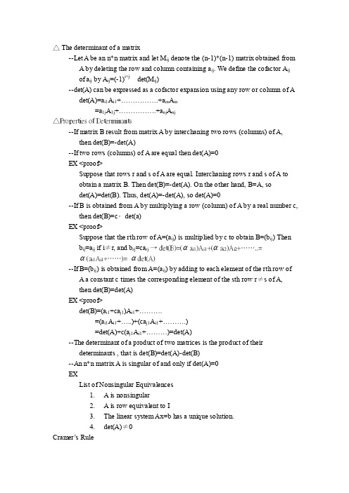
△ The determinant of a matrix--Let A be an n*n matrix and let M ij denote the (n-1)*(n-1) matrix obtained fromA by deleting the row and column containing a ij. We define the cofactor A ijof a ij by A ij=(-1)i+j det(M ij)--det(A) can be expressed as a cofactor expansion using any row or column of A det(A)=a i1A i1+…………….+a in A in=a1j A1j+…………….+a nj A nj△Properties of Determinants--If matrix B result from matrix A by interchaning two rows (columns) of A, then det(B)=-det(A)--If two rows (columns) of A are equal then det(A)=0EX <proof>Suppose that rows r and s of A are equal. Interchaning rows r and s of A toobtain a matrix B. Then det(B)=-det(A). On the other hand, B=A, sodet(A)=det(B). Thus, det(A)=-det(A), so det(A)=0--If B is obtained from A by multiplying a row (column) of A by a real number c, then det(B)=c∙det(a)EX <proof>Suppose that the rth row of A=(a ij) is multiplied by c to obtain B=(b ij) Thenb ij=a ij if i≠r, and b rj=ca rj→ det(B)=(αa i1)A i1+(αa i2)A i2+……..=α(a i1A i1+……)= αdet(A)--If B=(b ij) is obtained from A=(a ij) by adding to each element of the rth row ofA a constant c times the corresponding element of the sth row r≠s of A,then det(B)=det(A)EX <proof>det(B)=(a i1+ca j1)A i1+……….=(a i1A i1+…..)+(ca j1A i1+……….)=det(A)+c(a j1A i1+………)=det(A)--The determinant of a product of two matrices is the product of their determinants , that is det(B)=det(A)-det(B)--An n*n matrix A is singular of and only if det(A)=0EXList of Nonsingular Equivalences1. A is nonsingular2. A is row equivalent to I3.The linear system Ax=b has a unique solution.4.det(A)≠0Cramer’s Rule--Def Let A be an n*n matrix. We define a new matrix called the adjoint of A by⎥⎥⎥⎦⎤⎢⎢⎢⎣⎡=nn n n a a a a adjA ............1111 Thus to form the adjoint , we must replace each term by its cofactor and transpose the matrix--If A is nonsingular, then adjA A A )det(11=-ai1Aj1+ai2Aj2+…………ainAjn=det(A)→A(adjA)=det(A)I I adjA A A =))det(1(→adjA A A )det(11=- EX A=⎥⎥⎥⎦⎤⎢⎢⎢⎣⎡321223212adjA=[ ]= ⎥⎥⎥⎦⎤⎢⎢⎢⎣⎡---134247212⎥⎥⎥⎦⎤⎢⎢⎢⎣⎡---==-134247212)det(11adjA A A --Cramer ’s rule: Let A be an n*n nonsingular matrix, and also let A i be thematrix obtained by replacing the ith column of A by b. x is the unique solution to Ax=b then Xi=)det()det(A A i x=A -1b=b adjA A )()det(1 x i =)det()det()det(......2211A Ai A A b A b A b ni n i i =+++ EXx 1+2x 2+x 3=52x 1+2x 2+x 3=6x 1+2x 2+3x 3=9。
行列式的计算外文文献及翻译

1 The definition of determinant:n order determinant represented by the symbol nnn n nn a a a a a a a a a 212222111211n D =It represents the n!Algebra and items.These are all possible from different lines in different columns in the N element of the n nj j j a a a 2121 product.n nj j j a a a 2121symbols for )(21)1(n j j j τ-.When n j j j 21 iseven (odd) arrangement of the sign is positive (negative) .That is to sayn nn nj j j j j j j j j a a a 21212121)(n )1(D ∑-=τ.Here are∑nj j j 21 said the summation of all n order.Definition of determinant by inverse number given, should grasp the following four:(1) The total number of n order permutation is !n so the n order determinant expansion there are !n ;(2) Each item is taken from different lines, product of n elements in different columns;(3) The premise in subscript according to the natural number sequence, the parity of the inverse number each item in front of the sign depends on the column index consisting of the arrangement of the evidence, the other half, half of them take the negative; (4) A number is the value of determinant..Example 1: if the permutation inversions number n j j j 21 to I .How much is the inverse number and arrangement of 121j j j j n n -.Analysis:If the number of the original array.1j earlier than 1j large number of 1τ, a number of smaller than 1j number is 1)1(τ--n , and the number of new arrangement of 121j j j j n n -1j earlier than 1j large number of as 1)1(τ--n ; similarly, a number of the original arrangement set before 2j than 2j a large number of 2τ, a number of smaller than 2j number is2)2(τ--n , and the number of new arrangement of 2j earlier than 2j large number of as2)2(τ--n ; followed by analogy, a number of the original arrangement set before k j than k j large number of k τ, t he number of new arrangement in k j before the number greaterthan k j for ),,2,1()(n k k n k =--τ.Solution: a number of set the original permutation of k j than k j large number of k τ, a new arrangement ofk j earlier than k j large number of a number of),,2,1()(n k k n k =--τ. Because of I n =+++τττ 21 so Inverse numberarrangementof121j j j j n n - isI n n k n n n n nk k -=+++-+++-+-=--=-=∑2)1(211)(]01)2()1[(])[(τττττ2 basic theory2.1 Properties of n order determinantProperty 1: Transpose, determinant. That isnnn n n n a a a a a a a a a212222111211=nnn nn n a a a a a a a a a212221212111Property 2: a number multiplied by the determinant of a row is equal to the number is multipliedby this determinant. That is nnn n l l nnn n n l l n a a a a a a a a a k a a a ka ka ka a a a21ln 211121121ln 2111211= Nature 3: if a line is the two set of numbers and then the determinant equals two determinant and the determinant in addition to this, all with the original determinant of the correspondingline.nnn n n nnn n n n n nn n n n n n a a a c c c a a a a a a b b b a a a a a a c b c b c b a a a 21211121121211121121221111211+=+++ Nature 4: if the determinant of two lines of the same so determinant is zero. The so-called two lines of the same is corresponding elements of two lines of equal.Nature 5: if the determinant of the two line is proportional to the determinant is zero.02121ln 21112112121ln 2111211==nnn n in i i l l nnn n n in i i l l n a a a a a a a a a a a a k a a a a a a a a a a a aNature 6: the same row to another row determinant factor.Nature 7: to wrap column position in two lines of the determinant of No. 2.2 basic theory1 ⎩⎨⎧≠=+++0,0,2211ji D A a A a A a jn in j i j i Where ij A is a cofactor of element ij a . 2 Reduction theoremB CA D A DCB A 1--=3CA CB A =4B A AB =5 the nonzero matrix K left by a row to another row determinant is the new block determinant and the original equal2.3 results of several special determinant 1 triangular determinantnn nnn n a a a a a a a a a 221122211211000=(Triangular determinant )nn nnn n a a a a a a a a a221121222111000=(Lower triangular determinant )2 diagonal determinantnn nna a a a a a 221122110000=3 Symmetric and anti-symmetric determinantnnn n nn a a a a a a a a a D 212222111211=To meet the )2,1,2,1(n j n i a a ji ij ===, D is calledsymmetric determinant000331332312232111312 n n n n nn a a a a a a a a a a a a D =To meet the )2,1,(n j i a a ji ij =-=, D is calledskew-symmetric determinant. If the order of n is odd then 0=D 4 Vandermonde determinant∏≤<≤-----==ni j j i n n n n n nn n a a a a a a a a a a a a a a D 111312112232221321)(1111。
行列式的计算--中英文对照
行列式的计算摘 要:行列式是高等代数研究中的一个重要工具.本文从行列式的计算出发,通过例题,介绍行列式计算中的一些方法,同时初步给出了一些特殊行列式的计算方法,得出了一些关于行列式计算的技巧.关键词:行列式;三角化法;因式定理法;递推法;数学归纳法引 言行列式出现于线性方程组的求解,它最早是一种速记的表达式,现在已经是数学中一种非常有用的工具.行列式是由莱布尼茨和日本数学家关孝和发明的.同时代的日本数学家关孝和在其著作《解伏题元法》中也提出了行列式的概念与算法.1750年,瑞士数学家克拉默(1704-1752)在其著作《线性代数分析导引》中,对行列式的定义和展开法则给出了比较完整、明确的阐述,并给出了现在我们所称的解线性方程组的克拉默法则.稍后,数学家贝祖 (1730-1783)将确定行列式每一项符号的方法进行了系统化,利用系数行列式概念指出了如何判断一个齐次线性方程组有非零解.行列式是多门数学分支学科一个工具,在我们学习《高等代数》时,书中只介绍了几种较简单的行列式计算方法,但是在遇到比较复杂或技巧性比较强的行列式时,只局限于书上的几种方法,那解题就有点麻烦.这里我讨论了行列式计算的若干方法,针对不同的行列式来选择相对简单的计算方法,来提高解题的效率.1 基本概念的简单介绍 1.1 n 级行列式定义1]1[ n 级行列式nnn n n n a a a a a a a a a 212222111211 (1)等于所有取自不同行不同列的n 个元素的乘积n nj j j a a a 2121的代数和.其中n j j j 21是1,2,,n 的一个排列,n nj j j a a a 2121的每一项都按下列规则带有符号:当n j j j 21是偶排列时,n nj j j a a a 2121带有正号,当n j j j 21是奇排列时,n nj j j a a a 2121带有负号.1.2 矩阵在叙述行列式的重要公式和结论以及后面计算行列式过程中可能要用到矩阵及其有关概念,所以在这里简单介绍一下矩阵及其部分概念.定义2]1[ 由s n ⨯个数排成的s 行(横的)n 列(纵的)的表111212122212n n s s sn a a a a a a a a a ⎛⎫ ⎪ ⎪⎪⎪⎝⎭ (2)称为一个s n ⨯矩阵.特别地,当s n =时,(1)称为(2)的行列式,如果把(2)记作A ,则(1)表示为A .定义3]1[ 在行列式nnn n n n a a a a a a a a a 212222111211中划去元素ij a 所在的第i 行和第j 列后,剩下的2)1(-n 个元素按照原来的排法构成一个1-n 级行列式nnj n j n n ni j i j i i n i j i j i i n j j a a a a a a a a a a a a a a a a1,1,1,11,11,11,1,11,11,11,111,11,111+-+++-++-+----+- (3)称为元素ij a 的余子式,记作ij M ,而ij j i M +-)1(称为ij a 的代数余子式,记作:ij j i ij M A +-=)1( (4)定义4]1[ 我们把112111222212s s nnsn s na a a aa a a a a ⨯⎛⎫ ⎪ ⎪⎪ ⎪⎝⎭ (5) 称为矩阵(2)转置,记作A '或T A ,显然,s n ⨯矩阵的转置是n s ⨯矩阵.定义5]1[ 在一个n 级行列式D 中任意选定k 行k 列)(n k ≤位于这些行和列的交点上的2k 个元素按照原来的次序组成一个k 级行列式M ,称为行列式D 的一个k 级子式. 2 行列式的性质按照行列式的值可分为以下几类: 性质1 行列式值为01) 如果行列式有两行相同,则行列式值为0; 2) 如果行列式有两行成比例,则行列式值为0; 3) 行列式中有一行为0,则行列式的值为0. 性质2 行列式值不变1) 把一行的倍数加到另一行,行列式值不变, 即nnn n kn k k knin k i k i nnn n n kn k k in i i na a a a a a ca a ca a ca a a a a a a a a a a a a a a a a212122111121121212111211+++= (6) 其中R c ∈.2) 行列互换,行列式值不变, 即nnn n n n a a a a a a a a a 212222111211=nnn nn n a a a a a a a a a 212221212111 (7)3) 如果行列式的某一行是两组数的和,那么它就等于两个行列式的和, 这两个行列式除这一行外其余与原来行列式对应相同,即nnn n n n nn n n n n nn n n n n n a a a c c c a a a a a a b b b a a a a a a c b c b cb a a a21211121121211121121221111211+=+++(8)性质3 行列式的值改变 一行的公因子可以提出去,或者说用一数乘以行列式的一行就等于用该数乘以此行列式nnn n in i i nnn n n in i i n a a a a a a a a a k a a a ka ka ka a a a212111************= (9) 性质4 行列式反号对换行列式两行的位置,行列式反号nnn n in i i kn k k nnn n n kn k k in i i na a a a a a a a a a a a a a a a a a a a a a a a2121211121121212111211-= (10) 3 行列式的计算3.1 一些重要的公式和结论(1) 行列式按行(或列)展开设)(ij a A =为n 级方阵,ij A 为ij a 的代数余子式,则⎩⎨⎧≠==+++j i ji A A a A a A a jn in j i j i ,0,2211 (11)⎩⎨⎧≠==+++ji ji A A a A a A a nj ni j i j i ,0,2211 (12)(2) 设A 为n 级方阵,则A A T = (13)(3) 设A 为n 级方阵,则A k kA n = (14)(4) 设B A ,为n 级方阵,则B A AB =,但B A B A ±≠± (15)BA A B B A AB ===, (但一般地BA AB ≠)(16)(5) (拉普拉斯定理)设在n 级行列式D 中任意取定了)11(-≤≤n k k 个行,由这k 行元素所组成的一切k 级子式与它们的代数余子式的乘积的和等于行列式D .(6) 设A 为m 级方阵,B 为n 级方阵,则:00m m m n nnA A AB B B *==*,但是:0(1)0n mn m n mB A B A =- (17)(7) 德蒙德行列式1222212111112111()n n n j i i j nn n n nx x x D x x x x x x x x ≤<≤---==-∏(18)(8) 一些特殊行列式的值111222n nn λλλλλλλλλ***==***(19)对角行列式 上三角行列式 下三角行列式111222nnnλλλλλλλλλ***==***(20)次对角行列式 次上三角行列式 次下三角行列式 说明:(19)(20)中的行列式中*号处的元素不全为零. 3.2 低级行列式的计算 3.2.1 利用行列式定义,性质例1计算行列式y xyx x y x y y x y xD +++=3解:可以直接按照定义把行列式写开,得)(2))((233223y x y xy x y x D +-=-+-+=.3.2.2 利用三角化法例2 计算行列式3112321014D -= 解:利用三角化法:410550211411232113--=-=D 112(5)011014-=--112(5)01125005-=--=.3.3 n 级行列式的计算3.3.1 利用定义3.3.2 逐行(列)相减(加)法 3.3.3 利用因式定理法 3.3.4 递推降级法 3.3.5 拆分法3.3.6 数学归纳法3.3.7 利用公式和定理参考文献[1] 王萼芳,石生明.高等代数[M].大学数学系几何与代数教研室前代数小组编,1988.03.[2] 禾瑞,郝炳新.高等代数[M].高等教育, 1983.04.[3] 志慧,.高等代数分析与选讲[M].师大学数学与信息科学学院,2005.09.[4] 耿锁华.行列式性质的应用[M].审计学院, 2006.01.[5] 高丽,郭海清.两类特殊行历史的计算[M].西南民族大学, 2007.06.[6] 崇华.一类行列式的计算公式[M].大学, 2006.04.[7] 立英,成群.n级行列式的计算方法与技巧[M].师学院, 2006.01.[8] 清华,昊,金兰.高等代数容、方法与技巧[M].华中科技大学, 2006.08.[9] 毛纲源.线性代数解题方法技巧归纳(第二版)[M].华中理工大学, 2007.06.The calculation of determinantAbstractDeterminant is an important tool to study in higher algebra. In this paper, from the determinant calculation by examples, introduces some methods of determinant computation, at the same time, the preliminary calculation method is given. Some special determinant, draw some about the determinant calculation skills.KeywordsDeterminant; triangulation; factorization theorem; recursive method; mathematical inductionIntroductionSolving the determinant in linear equations, it is the first expression is a shorthand, now is a very useful tool in mathematics. The determinant is invented by Leibniz and the Japanese mathematician Seki takakazu. Contemporary Japanese mathematician Seki Takakazu in his book "V" thematic method solution also proposed the concept and algorithm of determinant.In 1750, the Swiss mathematician Cramer (1704-1752) in his book "linear algebra analysis guide", the definition of the determinant and expansion gives a relatively complete, clear, and gives now we call the solution of linear equations of the Cramer's rule. Later, the mathematician Bei Zu (17 30-1783) will determine the method of determinant each symbol is a systematic concept, using the coefficientdeterminant points out how to judge a homogeneous linear equations with non-zero solution.The determinant is one branch of mathematics as a tool, we learn in "Higher Algebra", the book describes only the determinant of some simple calculation methods, but in the face of the complicated or skills relatively strong determinant, several methods are confined to the book, the problem a bit of trouble. Here I discuss some methods for calculating determinant, the determinant to choose according to different method to calculate the relative simple, to improve the efficiency of problem solving.1 A brief introduction to the Basic Concepts1.1 n determinantDefines 1 levels of determinantnnn n nna a a a a a a a a 212222111211(1)Is equal to the algebraic sum of all taken from different lines of different column n elements of the product n nj j j a a a 2121 Where n j j j 21 is the 1, 2,…, n an order,n nj j j a a a 2121 each one of them according to the following rules with symbols: whenn j j j 21 is even permutation, with positive n nj j j a a a 2121, n j j j 21 when is oddpermutation, n nj j j a a a 2121 with a minus sign.1.2 matrixMay be used as matrix and its related concept in the process of thedeterminant of the determinant formula and conclusions and back calculation, so here is simple to introduce the concept of matrix and its parts.Definition 2 by the number of s n ⨯ into s lines (horizontal) n column(vertical) in Table 111212122212n n s s sn a a a a a a a a a ⎛⎫ ⎪ ⎪ ⎪ ⎪⎝⎭(2) Known as a s n ⨯ matrix. In particular, when s n =, (1) (2) is called the determinant, if (2) denoted as A, then (1) expressed as a ADefinition 3In the determinant ofnnn n nna a a a a a a a a 212222111211In return for element ij a in the i and j columns, the rest of the 2)1(-n elements according to the original method consisting of a n-1 determinantofnnj n j n n ni j i j i i n i j i j i i n j j a a a a a a a a a a a a a a a a1,1,1,11,11,11,1,11,11,11,111,11,111+-+++-++-+----+- (3).Known as the cofactor element ij atype, denoted as ij M , while theij j i M +-)1( is called the algebraic ij a type, denoted as:ij j i ij M A +-=)1((4).Definition 4 We call 112111222212s s nnsn s na a a a a a a a a ⨯⎛⎫ ⎪ ⎪⎪ ⎪⎝⎭ (5)Known as the matrix transpose (2), denoted as A ' or T A , apparently, transpose of s n ⨯ matrix is n s ⨯ .Definition 5 In n determinant of D in any of the selected k row k column)(n k ≤ is located in the intersection of these rows and columns of the 2k elements according to the original order in which a k determinant ofM, called a k step determinant of D type.2 Properties of the determinantAccording to the value of determinant can be divided into the following categories:(1) Properties of determinant value is 01) If there are two lines of the same determinant, the determinant value of 0;2) If the determinant is two in proportion, the determinant value of 0; 3) The determinant of a behavior of 0, the determinant of the value of 0(2) Properties of determinant.1) The line ratio to another line, the determinant of invariant, i.e.nnn n kn k k knin k i k i nnn n n kn k k in i i na a a a a a ca a ca a ca a a a a a a a a a a a a a a a a212122111121121212111211+++= (6) R c ∈2) Transpose, determinant value unchanged, i.e.nnn n n n a a a a a a a a a 212222111211=nnn nn n a a a a a a a a a 212221212111 (7)3) If a row determinant is two sets of numbers and, then it is equal tothe two determinant and the two determinant, in addition to the line outside the rest with the original determinant corresponding to the same, i.e.nnn n n n nn n n n n nn n n n n n a a a c c c a a a a a a b b b a a a a a a c b c b c b a a a21211121121211121121221111211+=+++ (8)(3)Change properties of determinantThe common factor line can be put forward to, or use a multiplied by the determinant of a is equal to the number is multiplied by this determinant nn n n in i i nnn n n in i i n a a a a a a a a a k a a a ka ka ka a a a212111************= (9) (4)Properties of determinant inverse numberOn line two, the number of determinantnnn n ini i knk k nnnn n knk k ini i na a a a a a a a a a a a a a a a a a a a a a a a2121211121121212111211-= (10) 3Calculation of determinant3.1 Some important formulas and conclusions(1) The determinant line (or column) expansionLet )(ij a A = be n matrix, the ij A cofactor ij a type, then⎩⎨⎧≠==+++ji ji A A a A a A a jn in j i j i ,0,2211 (11)⎩⎨⎧≠==+++j i ji A A a A a A a nj ni j i j i ,0,2211 (12)(2) Let A be a n matrix,AA T =(13)(3) Let A be a n matrix,Ak kA n =(14)(4) Let A, B is n matrix, B A AB =,但B A B A ±≠± (15)BA A B B A AB ===, (, but generally BA AB ≠ ) (16) (5) (Laplasse theorem) In arbitrary n determinant of D in the)11(-≤≤n k k line, product of algebraic all k type consisted of the kelements and their type and is equal to the determinant of D. (6) Let A be a m matrix, B matrix, n,0m m m n n nA A AB B B *==*But,0(1)0n mn m n mB A B A =- (17)(7) Van Redmond determinant1222212111112111()n n n j i i j nn n n nx x x D x x x x x x x x ≤<≤---==-∏(18).(8) Some special determinant value111222n nn λλλλλλλλλ***==***(19)111222nnnλλλλλλλλλ***==***(20).Notes: (19) (20) of the determinant of the elements * are not all zero.3.2Calculation of primary determinant3.2.1 Use of the definition of the determinant, properties 1 cases of computing determinant ofy xyx x y x y y x y xD +++=3Solution: can be directly according to the definition of the determinant is written,)(2))((233223y x y xy x y x D +-=-+-+=.3.2.2 Uses triangulation method2 cases of computing determinant of3112321014D -= Solution : the use of triangulation method410550211411232113--=-=D 112(5)011014-=--112(5)0112505-=--=3.3Calculation of level n determinant3.3.1Using the definition3.3.2 Row (column) subtract (add) method 3.3.3 Factor theorem method3.3.4The recursive degradation method 3.3.5 Method3.3.6 Mathematical induction3.3.7Using the formula and theoremReference[1] Wang Efang, Ihi Kim algebraic geometry and higher algebra [M]. Department of Peking University Department of mathematics of algebra group coding,1988.03.[2] Zhang Herui, Hao Bingxin. Advanced algebra [M]. Beijing higher education press, 1983.04.[3] Li Zhihui, Li Yongming and [M]. Of Shaanxi Normal University College of mathematics and information science of higher algebra,2005.09.[4] Geng Suohua. The determinant of the nature of the application [M]. Nanjing Audit University press, 2006.01.[5] Korea, Guo Haiqing. Calculation of [M]. Southwest University forNationalities press two kinds of special line history, 2007.06.[6] Liu Chonghua. A class of determinantal formula for [M]. Nanning University Press, 2006.04.[7] Yang Liying, Li Chengqun. Calculation methods and skills of primary determinant [M]. Guangxi Teachers Education University press, 2006.01.[8] Sun Qinghua, Sun Hao, Li Jinlan and skill of Higher Algebra content, method of [M]. Huazhong University of Science and Technology press, 2006.08.[9] Hair Gangyuan linear algebra problem solving methods. Techniques (Second Edition) [M]. Huazhong University of science and Technology Press, 2007.06.。
行列式的计算方法文献综述
行列式的计算方法摘要:本文叙述了行列式的发展历程,现状和研究方法分析。
概述了一些计算方法,最后提出一些行列式的计算方法值得进一步探讨的问题。
关键词 :行列式;方程组;计算方法;加边法1. 引言行列式是人们为了研究二、三元的线性方程组而创建的,它是大学数学学习的一个重要内容,是求解线性方程组,求逆矩阵及求矩阵特征值的基础。
而它的应用并不止局限于代数的范围,它也是许多其他学科研究的重要工具,如行列式经常被用于涉及到的电子工程、控制论、数学物理方程的研究等。
而行列式的计算具有一定的规律性和技巧性,综合性较强,在行列式计算中需要我们多观察总结,才能更熟练地计算出行列式的值。
在行列式的计算过程中,不同特征的行列式适用不同的方法,每一种方法都有它们各自的优点及其独特之处,因此具有非常重要的研究价值。
本论文主要从2000 年到2012 年发表的若干期刊中,总结出行列式的计算的发展历程、现状以及研究的方向。
2. 正文2.1行列式的历史:行列式的概念最初是因方程组的求解而发展起来的,它的提出是在十七世纪,由日本数学家关孝和与德国数学家戈特弗里德·莱布尼茨各自独立得出,那时已经使用行列式来确定线性方程组解的个数以及形式。
十八世纪开始,行列式开始作为独立的数学概念被研究。
1750 年,瑞士数学家克莱姆在其著作《线性代数分析导引》中,对行列式的定义和展开法则给出了比较完整、明确的阐述,并给出了现在我们所称的解线性方程组的克莱姆法则。
后来,数学家贝祖将确定行列式每一项符号的方法进行了系统化,利用系数行列式概念指出了如何判断一个齐次线性方程组有非零解。
1772 年,拉普拉斯在一篇论文中证明了范德蒙提出的一些规则,推广了他的展开行列式的方法。
十九世纪以后,行列式理论进一步得到发展和完善。
1815 年,柯西在一篇论文中给出了行列式的第一个系统的处理,其中主要结果之一是行列式的乘法定理。
1841年,雅可比发表了一篇关于函数行列式的论文,讨论函数的线性相关性与雅可比行列式的关系。
线代名词中英文对照

38
the determinant of matrix A
方阵A的行列式
39
operations on Matrices
矩阵的运算
40
a transposed matrix
转置矩阵
41
an inverse matrix
逆矩阵
42
an conjugate matrix
共轭矩阵
43
an diagonal matrix
线性组合
51
space of arithmetical vectors
向量空间
52
subspace
子空间
53
dimension
维
54
basis
基
55
canonical basis
规范基
56
coordinates
坐标
57
decomposition
分解
58
transformation matrix
过渡矩阵
正交化过程
93
reducing a matrix to the diagonal form
对角化矩阵
94
orthonormal basis
标准正交基
95
orthogonal transformation
正交变换
96
linear transformation
线性变换
97
quadratic forms
二次型
坐标变换
对角矩阵
44
an adjoint matrix
伴随矩阵
45
singular matrix
奇异矩阵
- 1、下载文档前请自行甄别文档内容的完整性,平台不提供额外的编辑、内容补充、找答案等附加服务。
- 2、"仅部分预览"的文档,不可在线预览部分如存在完整性等问题,可反馈申请退款(可完整预览的文档不适用该条件!)。
- 3、如文档侵犯您的权益,请联系客服反馈,我们会尽快为您处理(人工客服工作时间:9:00-18:30)。
1 The definition of determinant:n order determinant represented by the symbol nnn n nn a a a a a a a a a 212222111211n D =It represents the n!Algebra and items.These are all possible from different lines in different columns in the N element of the n nj j j a a a 2121 product.n nj j j a a a 2121symbols for )(21)1(n j j j τ-.When n j j j 21 iseven (odd) arrangement of the sign is positive (negative) .That is to sayn nn nj j j j j j j j j a a a 21212121)(n )1(D ∑-=τ.Here are∑nj j j 21 said the summation of all n order.Definition of determinant by inverse number given, should grasp the following four:(1) The total number of n order permutation is !n so the n order determinant expansion there are !n ;(2) Each item is taken from different lines, product of n elements in different columns;(3) The premise in subscript according to the natural number sequence, the parity of the inverse number each item in front of the sign depends on the column index consisting of the arrangement of the evidence, the other half, half of them take the negative; (4) A number is the value of determinant..Example 1: if the permutation inversions number n j j j 21 to I .How much is the inverse number and arrangement of 121j j j j n n -.Analysis:If the number of the original array.1j earlier than 1j large number of 1τ, a number of smaller than 1j number is 1)1(τ--n , and the number of new arrangement of 121j j j j n n -1j earlier than 1j large number of as 1)1(τ--n ; similarly, a number of the original arrangement set before 2j than 2j a large number of 2τ, a number of smaller than 2j number is2)2(τ--n , and the number of new arrangement of 2j earlier than 2j large number of as2)2(τ--n ; followed by analogy, a number of the original arrangement set before k j than k j large number of k τ, t he number of new arrangement in k j before the number greaterthan k j for ),,2,1()(n k k n k =--τ.Solution: a number of set the original permutation of k j than k j large number of k τ, a new arrangement ofk j earlier than k j large number of a number of),,2,1()(n k k n k =--τ. Because of I n =+++τττ 21 so Inverse numberarrangementof121j j j j n n - isI n n k n n n n nk k -=+++-+++-+-=--=-=∑2)1(211)(]01)2()1[(])[(τττττ2 basic theory2.1 Properties of n order determinantProperty 1: Transpose, determinant. That isnnn n n n a a a a a a a a a212222111211=nnn nn n a a a a a a a a a212221212111Property 2: a number multiplied by the determinant of a row is equal to the number is multipliedby this determinant. That is nnn n l l nnn n n l l n a a a a a a a a a k a a a ka ka ka a a a21ln 211121121ln 2111211= Nature 3: if a line is the two set of numbers and then the determinant equals two determinant and the determinant in addition to this, all with the original determinant of the correspondingline.nnn n n n nn n n n n nn n n n n n a a a c c c a a a a a a b b b a a a a a a c b c b c b a a a 21211121121211121121221111211+=+++ Nature 4: if the determinant of two lines of the same so determinant is zero. The so-called two lines of the same is corresponding elements of two lines of equal.Nature 5: if the determinant of the two line is proportional to the determinant is zero.02121ln21112112121ln 2111211==nnn n ini i l l n nn n n ini i l l n a a a a a a a a a a a a k a a a a a a a a a a a aNature 6: the same row to another row determinant factor.Nature 7: to wrap column position in two lines of the determinant of No. 2.2 basic theory1 ⎩⎨⎧≠=+++0,0,2211ji D A a A a A a jn in j i j i Where ij A is a cofactor of element ij a . 2 Reduction theoremB CA D A DCB A 1--=3CA CB A =4B A AB =5 the nonzero matrix K left by a row to another row determinant is the new block determinant and the original equal2.3 results of several special determinant 1 triangular determinantnn nnn n a a a a a a a a a 221122211211000=(Triangular determinant )nn nnn n a a a a a a a a a221121222111000=(Lower triangular determinant )2 diagonal determinantnn nna a a a a a 221122110000=3 Symmetric and anti-symmetric determinantnnn n nn a a a a a a a a a D 212222111211=To meet the )2,1,2,1(n j n i a a ji ij ===, D is calledsymmetric determinant000331332312232111312 n n n n nn a a a a a a a a a a a a D =To meet the )2,1,(n j i a a ji ij =-=, D is calledskew-symmetric determinant. If the order of n is odd then 0=D 4 Vandermonde determinant∏≤<≤-----==ni j j i n n n n n nn n a a a a a a a a a a a a a a D 111312112232221321)(1111。