Tikhonov吉洪诺夫正则化
正则化原理总结
正则化原理总结正则化理论(Regularization Theory)是 Tikhonov于1963年提出的⼀种⽤以解决逆问题的不适定性的⽅法。
不适定性通常由⼀组线性代数⽅程定义,这组⽅程组由于具有很⼤的系数⽽使得它的反问题(已知系统输出求输⼊)存在多解。
正则化理论就是⽤来对原始问题的最⼩化经验误差函数(损失函数)加上某种约束,这种约束可以看成是⼈为引⼊的某种先验知识(正则化参数等价于对参数引⼊先验分布),从⽽对原问题中参数的选择起到引导作⽤,因此缩⼩了解空间,也减⼩了噪声对结果的影响和求出错误解的可能,使得模型由多解变为更倾向其中⼀个解。
也就是说,正则化项本质上是⼀种先验信息,整个最优化问题从贝叶斯观点来看是⼀种贝叶斯最⼤后验估计,其中正则化项对应后验估计中的先验信息(不同的正则化项具有不同先验分布),损失函数对应后验估计中的似然函数,两者的乘积则对应贝叶斯最⼤后验估计的形式。
附加的先验信息强⾏地让系统学习到的模型具有⼈们想要的特性,例如稀疏、低秩、平滑等等,约束了梯度下降反向迫使最终解倾向于符合先验知识。
接下来的问题是我们应该引⼊什么样正则项作为先验知识,才能准确⾼效地缩⼩解空间?⼀切⽅法的动机来源于⼈们⼀直以来对科学的“简洁性”、“朴素性”和“美”的深刻认同,这⼀经典理念可以⽤14世纪逻辑学家Occam提出的“奥克姆剃⼑”原理表述,它长久以来被⼴泛运⽤在⼈们对⾃然科学、社会科学的探索和假设之中:Entities should not be multiplied unnecessarily,译作“若⽆必要,勿增实体”,即“简单有效原理”。
说到这⾥还想多说⼏句题外话。
其实⾄少从亚⾥⼠多德以来,在哲学界、科学界陆续有很多⼈针对不同的场景、以种种⽅式提出了类似的观点。
科学家们⽤这种⽅式,作为建⽴基本假设的原则、作为想象⼒的出发点和思考的⼤⽅向、作为模型选择和建⽴的依据,最终得到了被实验事实所验证的理论学说,⽐如:⽜顿经典⼒学、麦克斯韦⽅程中位移电流的假设、进化论中进化机制的构想、狭义相对论两个基本假设的建⽴、⼴义相对论场⽅程的推导等等,当然它在如今的管理学、经济学等领域同样被⼴泛运⽤。
【国家自然科学基金】_tikhonov正则化方法_基金支持热词逐年推荐_【万方软件创新助手】_20140729
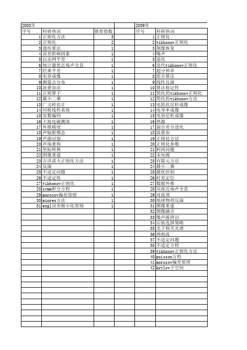
科研热词 正则化 tikhonov正则化 图像恢复 噪声 退化 迭代tikhonov正则化 超分辨率 组合算法 线性反演 算法稳定性 简化的tikhonov正则化 简化的tikhonov方法 电阻抗层析成像 电导率成像 电容层析成像 热源 混合差分进化 波叠加 正则化方法 正则化参数 柯西问题 未知源 有限元方法 最小二乘 最优控制 时差定位 数据外推 局部近场声全息 对流项 地球物理反演 图像重建 图像融合 噪声源辨识 后验选择策略 光子相关光谱 两相流 不适定问题 不适定方程 tikhonov正则化方法 poisson方程 morozov偏差原理 krylov子空间
2008年 序号 1 2 3 4 5 6 7 8 9 10 11 12 13 14 15 16 17 18 19 20 21 22 23 24 25 26 27 28 29 30 31
科研热词 正则化方法 正则化 遗传算法 误差影响因素 自由网平差 统计最优近场声全息 经典平差 电容成像 测量点分布 波叠加法 正则算子 最小二乘 广义岭估计 对称线性系统 实数编码 大地电磁测深 外推精度 声辐射模态 声源识别 声场重构 坐标转换 图像重建 吉洪诺夫正则化方法 反演 不适定问题 不适定性 tikhonov正则化 symm积分方程 morozov偏差原则 minres方法 engl误差极小化原则
科研热词 推荐指数 正则化 8 简化的tikhonov方法 2 热源 2 时域有限差分 2 对流项 2 tikhonov正则化 2 鲁棒性 1 高度计 1 风场调整 1 非线性 1 静态储备池 1 逆散射 1 边界温度场 1 转换矩阵 1 色散介质 1 维纳去卷积 1 精细算法 1 算法 1 第一类fredholm积分方程 1 离散小波变换 1 电导率成像 1 热传导方程 1 正则化参数 1 模型修正 1 最小二乘法 1 时变结构 1 支持向量回归 1 损伤识别 1 拟逆 1 抛物方程 1 微波断层成像 1 差分进化算法 1 小波有限元法 1 多尺度分析 1 多宗量 1 反问题 1 反应成份 1 参数识别 1 区间b样条小波 1 动态规划技术 1 加权bregman函数 1 刺激成份 1 事件相关电位 1 乳腺癌 1 不适定问题 1 tikhonov正则化方法 1 newton算法 1 newton插值 1 l曲线 1 legendre小波 1 kriging插值 1 kaula 1
吉洪诺夫正则化方法
吉洪诺夫正则化方法
吉洪诺夫正则化方法是一种常用的数据处理方法,用于处理数据中存在的噪声和异常值。
该方法通过在损失函数中添加一个正则化项,来限制模型参数的大小,从而达到减少过拟合的效果。
吉洪诺夫正则化方法的基本思想是,在损失函数中添加一个正则化项,该正则化项包括模型参数的平方和,以及一个正则化系数。
该正则化系数越大,就越能限制模型参数的大小,从而减少过拟合的风险。
使用吉洪诺夫正则化方法可以避免模型在训练集上表现良好,但在测试集上表现不佳的情况。
因为该方法可以使得模型更加平滑,减少过拟合风险,从而提高模型的泛化能力。
吉洪诺夫正则化方法常用于线性回归、逻辑回归、支持向量机等模型的训练过程中,可以通过交叉验证等方法来确定正则化系数的大小。
- 1 -。
地球物理反演中的正则化技术分析

地球物理反演中的正则化技术分析地球物理反演是一种通过观测地球上各种现象和数据,来推断地球内部结构和物质分布的方法。
在地球物理反演中,由于观测数据的不完整性和不精确性,常常需要借助正则化技术来提高反演结果的可靠性和准确性。
正则化技术是一种以一定规则限制解的优化方法。
通过在反演过程中引入附加信息或者假设,正则化技术可以帮助减小反演问题的不确定性,提高解的稳定性和可靠性。
在地球物理反演中,正则化技术有多种应用。
下面将介绍几种常见的正则化技术,并对其进行分析和比较。
1. Tikhonov正则化Tikhonov正则化是一种基本的正则化技术,它通过在目标函数中加入一个范数约束来限制解的空间。
常见的约束可以是L1范数和L2范数。
L1范数可以使解具有稀疏性,即解中的大部分分量为零,适用于具有稀疏特性的反演问题。
而L2范数可以使解具有平滑性,适用于具有平滑特性的反演问题。
2. 主成分分析正则化主成分分析正则化是一种通过将反演问题映射到低维空间来减小问题的维度的正则化技术。
它可以通过选择重要的主成分来实现数据降维,从而减少反演问题的不确定性。
主成分分析正则化在处理高维数据时可以提高反演的效率和精度。
3. 奇异值正则化奇异值正则化是一种基于奇异值分解的正则化技术。
通过对反演问题进行奇异值分解,可以将问题分解为多个低维子问题,从而减小高维问题的不确定性。
奇异值正则化适用于非线性反演问题,可以提高反演结果的稳定性和可靠性。
4. 稀疏表示正则化稀疏表示正则化是一种基于稀疏表示理论的正则化技术。
它通过将反演问题转化为对系数矩阵的优化问题,并引入L1范数约束,使得解具有稀疏性。
稀疏表示正则化适用于信号重构和图像恢复等问题,并在地震勘探和地球成像中有广泛应用。
在选择正则化技术时,需要考虑问题的特性和数据的特点。
不同的正则化技术适用于不同的问题,并且各自具有一些优势和限制。
因此,根据问题的具体要求和数据的特征,选择合适的正则化技术可以提高反演结果的可靠性和准确性。
tikhonov正则化matlab程序
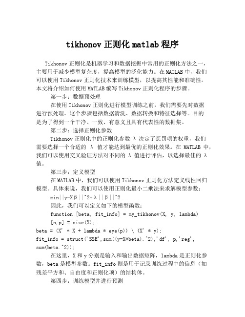
tikhonov正则化matlab程序Tikhonov正则化是机器学习和数据挖掘中常用的正则化方法之一,主要用于减少模型复杂度,提高模型的泛化能力。
在MATLAB中,我们可以使用Tikhonov正则化技术来训练模型,以提高其性能和准确性。
本文将介绍如何使用MATLAB编写Tikhonov正则化程序的步骤。
第一步:数据预处理在使用Tikhonov正则化进行模型训练之前,我们需要先对数据进行预处理。
这个步骤包括数据清洗、数据转换和特征选择等。
目的是为了得到一个干净、一致、有意义且具有代表性的数据集。
第二步:选择正则化参数Tikhonov正则化中的正则化参数λ决定了惩罚项的权重,我们需要选择一个合适的λ值才能达到最优的正则化效果。
在MATLAB中,我们可以使用交叉验证方法对不同的λ值进行评估,以选择最佳的λ值。
第三步:定义模型在MATLAB中,我们可以使用Tikhonov正则化方法定义线性回归模型。
具体来说,我们可以使用正则化最小二乘法来求解模型参数:min||y-Xβ||^2+λ||β||^2因此,我们可以定义如下的模型函数:function [beta, fit_info] = my_tikhonov(X, y, lambda)[n,p] = size(X);beta = (X' * X + lambda * eye(p)) \ (X' * y);fit_info = struct('SSE',sum((y-X*beta).^2),'df', p,'reg',sum(beta.^2));在这里,X和y分别是输入和输出数据矩阵,lambda是正则化参数,beta是模型参数。
fit_info则是用于记录训练过程中的信息(如残差平方和、自由度和正则化项)的结构体。
第四步:训练模型并进行预测在定义好模型函数之后,我们可以使用MATLAB中的训练函数来训练模型,并使用测试函数进行预测。
迭代吉洪诺夫正则化的FCM聚类算法

迭代吉洪诺夫正则化的FCM聚类算法蒋莉芳;苏一丹;覃华【摘要】模糊C均值聚类算法(fuzzy C-means,FCM)存在不适定性问题,数据噪声会引起聚类失真.为此,提出一种迭代Tikhonov正则化模糊C均值聚类算法,对FCM的目标函数引入正则化罚项,推导最优正则化参数的迭代公式,用L曲线法在迭代过程中实现正则化参数的寻优,提高FCM的抗噪声能力,克服不适定问题.在UCI 数据集和人工数据集上的实验结果表明,所提算法的聚类精度较传统FCM高,迭代次数少10倍以上,抗噪声能力更强,用迭代Tikhonov正则化克服传统FCM的不适定问题是可行的.%FCM algorithm has the ill posed problem.Regularization method can improve the distortion of the model solution caused by the fluctuation of the data.And it can improve the precision and robustness of FCM through solving the error estimate of solution caused by ill posed problem.Iterative Tikhonov regularization function was introduced into the proposed problem (ITR-FCM),and L-curve method was used to select the optimal regularization parameter iteratively,and the convergence rate of the algorithm was further improved using the dynamic Tikhonov method.Five UCI datasets and five artificial datasets were chosen for the test.Results of tests show that iterative Tikhonov is an effective solution to the ill posed problem,and ITR-FCM has better convergence speed,accuracy and robustness.【期刊名称】《计算机工程与设计》【年(卷),期】2017(038)009【总页数】5页(P2391-2395)【关键词】模糊C均值聚类;不适定问题;Tikhonov正则化;正则化参数;L曲线【作者】蒋莉芳;苏一丹;覃华【作者单位】广西大学计算机与电子信息学院,广西南宁 530004;广西大学计算机与电子信息学院,广西南宁 530004;广西大学计算机与电子信息学院,广西南宁530004【正文语种】中文【中图分类】TP389.1模糊C均值算法已广泛地应用于图像分割、模式识别、故障诊断等领域[1-6]。
tikhonov正则化方法
tikhonov正则化方法Tikhonov正则化方法是一种用于解决线性反问题的数值稳定方法,也称为Tikhonov-Miller方法或Tikhonov-Phillips方法。
它由俄罗斯数学家Andrey Tikhonov在20世纪40年代提出,被广泛应用于信号处理、图像处理、机器学习、物理学等领域。
线性反问题指的是,给定一个线性方程组Ax=b,已知矩阵A和向量b,求解未知向量x。
然而,在实际应用中,往往存在多个解或无解的情况,而且解的稳定性和唯一性也很难保证。
这时候,就需要引入正则化方法来提高求解的稳定性和精度。
Tikhonov正则化方法的基本思想是,在原有的线性方程组中添加一个正则化项,使得求解的解更加平滑和稳定。
具体地说,Tikhonov 正则化方法可以用下面的形式表示:min ||Ax-b||^2 + λ||x||^2其中,第一项表示原有的误差项,第二项表示正则化项,λ是正则化参数,用来平衡两个项的重要性。
当λ越大时,正则化项的影响就越大,求解的解就越平滑和稳定;当λ越小时,误差项的影响就越大,求解的解就越接近原有的线性方程组的解。
Tikhonov正则化方法的求解可以通过最小二乘法来实现。
具体地说,可以将原有的线性方程组表示为Ax=b的形式,然后将其转化为最小二乘问题,即:min ||Ax-b||^2然后,再添加一个正则化项λ||x||^2,得到Tikhonov正则化问题。
由于这是一个二次最小化问题,可以通过求导等方法来求解。
Tikhonov正则化方法的优点在于,它可以有效地提高求解的稳定性和精度,减少过拟合和欠拟合的问题。
同时,它的求解也比较简单和直观,适用于各种线性反问题的求解。
然而,Tikhonov正则化方法也存在一些限制和局限性。
首先,正则化参数λ的选择比较困难,需要通过试错和经验来确定;其次,正则化项的形式也比较单一,往往不能很好地适应不同的问题和数据;最后,Tikhonov正则化方法只适用于线性反问题的求解,对于非线性问题和大规模问题的求解效果较差。
采用边界积分方程和tikhonov正则化方法延拓潜艇磁场
采用边界积分方程和tikhonov正则化方法延拓潜艇磁场边界积分方程和Tikhonov正则化方法是一种有效的手段,用于延拓潜艇磁场。
这种方法基于物理学原理和数学模型,可以通过计算潜艇表面的磁场分布,来推断潜艇内部的磁场分布。
本文将详细介绍这种方法的原理和应用。
一、边界积分方程边界积分方程是一种数学工具,用于描述物体表面的电磁场分布。
在潜艇磁场延拓中,我们可以将潜艇表面看作一个电磁场边界,通过边界积分方程来计算潜艇表面的磁场分布。
具体来说,我们可以将潜艇表面划分成若干个小面元,对每个小面元上的磁场进行积分,得到整个表面上的磁场分布。
这种方法可以有效地避免对潜艇内部结构的复杂计算,从而简化了问题的求解。
二、Tikhonov正则化方法Tikhonov正则化方法是一种数学工具,用于处理反问题。
在潜艇磁场延拓中,我们需要通过已知的潜艇表面磁场分布,来推断潜艇内部的磁场分布。
这是一个反问题,通常会受到噪声和不确定性的影响。
Tikhonov正则化方法可以通过引入正则化项,来限制解的复杂度,从而提高解的稳定性和精度。
三、应用实例潜艇磁场延拓方法在实际应用中具有广泛的应用价值。
例如,在海洋探测和海底勘探中,可以通过潜艇磁场延拓方法来推断海底地形和地质构造。
在潜艇隐身技术中,可以通过潜艇磁场延拓方法来预测潜艇的磁场特征,从而减少被敌方探测的可能性。
此外,潜艇磁场延拓方法还可以应用于磁共振成像、地球物理勘探等领域。
总之,边界积分方程和Tikhonov正则化方法是一种有效的手段,用于延拓潜艇磁场。
这种方法基于物理学原理和数学模型,可以通过计算潜艇表面的磁场分布,来推断潜艇内部的磁场分布。
在实际应用中,潜艇磁场延拓方法具有广泛的应用价值,可以为海洋探测、潜艇隐身技术、磁共振成像、地球物理勘探等领域提供有力的支持。
Tikhonov正则化参数的选取及两类反问题的研究的开题报告
Tikhonov正则化参数的选取及两类反问题的研究的开题报告题目:Tikhonov正则化参数的选取及两类反问题的研究一、研究背景和意义:随着科学技术的进步,反问题研究成为了最热门的研究领域之一。
反问题的研究涉及到的学科领域非常广泛,其中数学、物理和工程等领域是最为重要的。
反问题包括了许多子领域,如参数反问题、区域反问题、混合反问题等等。
其中参数反问题是最为基础和重要的子领域之一。
Tikhonov正则化方法在参数反问题中得到了广泛应用,因为它可以通过降低噪声波动和提高解的光滑性来改进问题的稳定性。
然而,在应用Tikhonov正则化方法时,如何选取正则化参数是一个非常重要的问题,因为不同的正则化参数会影响到结果的精度和稳定性。
此外,不同类型的反问题需要对正则化参数作出不同的选择,这也是一个需要进一步探究的问题。
因此,我们需要对Tikhonov正则化参数的选取以及在不同类型的反问题中的应用进行深入的研究。
二、研究内容和目标:本文将主要研究Tikhonov正则化参数的选取方法,探讨其在参数反问题和区域反问题中的应用。
具体研究内容包括以下几个方面:1. 对Tikhonov正则化方法的优化算法进行研究,包括最小二乘方法、正交匹配迭代算法等。
2. 针对参数反问题,研究不同类型的Tikhonov正则化方法与对应的正则化参数的选取方法,并比较其性能和精度。
3. 针对区域反问题,研究不同类型的Tikhonov正则化方法与对应的正则化参数的选取方法,并比较其性能和精度。
4. 开发相应的计算程序,实现研究结果的数值验证和实际应用。
通过以上研究,本文旨在实现以下目标:1. 系统性地总结不同类型的Tikhonov正则化方法与对应的正则化参数的选取方法,并探讨其适用范围和局限性。
2. 比较不同类型的Tikhonov正则化方法及其选取的正则化参数在参数反问题和区域反问题中的应用效果,提出相应改进措施,提高解的稳定性和精度。
3. 开发相应的计算程序,实现研究结果的数值验证和实际应用,为相关领域的研究提供参考。
吉洪诺夫正则化与lm算法的区别
吉洪诺夫正则化与lm算法的区别摘要::1.引言2.吉洪诺夫正则化与lm算法的概念解释3.吉洪诺夫正则化与lm算法的区别4.两者在实际应用中的优劣势5.总结正文:吉洪诺夫正则化与lm算法的区别在机器学习和统计建模领域,吉洪诺夫正则化(Tikhonov Regularization)和最小二乘法(Least Mean Squares,简称lm算法)是两种常见的优化方法。
它们在解决线性回归问题等方面具有一定的相似性,但也存在明显的差异。
本文将详细介绍这两种算法的概念、区别以及在实际应用中的优劣势。
1.引言在许多实际问题中,我们都需要从观测数据中拟合一个线性模型,以便对未知参数进行估计。
然而,由于观测数据的噪声和模型本身的复杂性,直接求解参数往往面临病态问题的困扰。
吉洪诺夫正则化和lm算法正是为了解决这一问题而提出的。
2.吉洪诺夫正则化与lm算法的概念解释吉洪诺夫正则化是一种在求解病态问题时采用的优化方法。
它通过在目标函数中增加一个正则项来约束解的稳定性,从而使得求解过程更加稳定。
正则项的选取与问题相关,常见的有L1、L2正则化。
lm算法,又称最小二乘法,是一种通过最小化目标函数(平方误差)来求解线性回归模型参数的方法。
它是一种无偏估计方法,可以得到参数的一致估计。
3.吉洪诺夫正则化与lm算法的区别吉洪诺夫正则化和lm算法的本质区别在于它们在求解过程中对解的稳定性约束方式不同。
吉洪诺夫正则化是通过在目标函数中增加正则项来约束解的稳定性,而lm算法是通过最小化目标函数来自然地保证解的稳定性。
因此,吉洪诺夫正则化更适用于解决病态问题,而lm算法在一般情况下也能得到较好的结果。
4.两者在实际应用中的优劣势在实际应用中,吉洪诺夫正则化和lm算法各有优劣势。
吉洪诺夫正则化具有较强的鲁棒性,可以应对病态问题,但计算复杂度较高;而lm算法计算简便,但在面临病态问题时可能收敛速度较慢或得不到稳定解。
因此,在选择算法时,需要根据实际问题的特点进行权衡。
正则化参数的确定方法
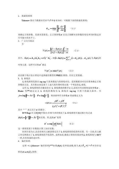
1. 拟最优准则Tikhonov 指出当数据误差水平δ和η未知时,可根据下面的拟最优准则:0min opt dx d ααααα>⎧⎫⎪⎪=⎨⎬⎪⎪⎩⎭(1-1) 来确定正则参数。
其基本思想是:让正则参数α以及正则解对该参数的变化率同时稳定在尽可能小的水平上。
2. 广义交叉验证令22(())/()[(())]/I A y m V tr I A mδααα-=- (2-1) 其中,*1*()A (A A I)A h h h h A αα-=+,1(I A())(1())mkk k tr ααα=-=-∑,()kk αα为()A α的对角元素。
这样可以取*α满足 *()min ()V V αα= (2-2)此法源于统计估计理论中选择最佳模型的PRESS 准则,但比它更稳健。
3. L_曲线法L 曲线准则是指以log-log 尺度来描述与的曲线对比,进而根据该对比结果来确定正则 参数的方法。
其名称由来是基于上述尺度作图时将出现一个明显的L 曲线。
运用L 曲线准则的关键是给出L 曲线偶角的数学定义,进而应用该准则选取参数α。
Hanke 等[64]建议定义L 曲线的偶角为L 曲线在log-log 尺度下的最大曲率。
令log b Ax αρ=-,log x αθ=,则该曲率作为参数α的函数定义为''''''3'2'22()(()())c ρθρθαρθ-=+ (3-1)其中“'”表示关于α的微分。
H.W.Engl 在文献[40]中指出:在相当多的情况下,L 曲线准则可通过极小化泛函()x b Ax ααφα=-来实现。
即,选取*α使得{}*0arg inf ()ααφα>= (3-2) 这一准则更便于在数值计算上加以实施。
但到目前为止,还没有相关文献获得过关于L 曲线准则的收敛性结果。
另一方面,有文献己举反例指出了L 曲线准则的不收敛性。
吉洪诺夫正则化矩阵
吉洪诺夫正则化矩阵
吉洪诺夫正则化矩阵是一种常用的矩阵变换方法,它可以用于降低矩阵的条件数,从而提高矩阵求解的稳定性和精度。
该方法的基本思想是将原始矩阵加上一个正定对称矩阵的某个倍数,从而得到一个新的正定对称矩阵,这个新矩阵的条件数会比原始矩阵小很多。
具体来说,对于一个实对称矩阵A,吉洪诺夫正则化矩阵可以表示为:
A' = A + alpha * I
其中,alpha是一个正实数,I是单位矩阵。
这里的alpha通常取值为原始矩阵A的特征值中的最小正实数,以确保A'是正定对称矩阵。
通过这种方式,我们可以有效地降低矩阵A'的条件数,从而提高矩阵求解的稳定性和精度。
吉洪诺夫正则化矩阵在数值线性代数中应用广泛,尤其是在求解线性方程组和特征值问题时。
它不仅可以用于稠密矩阵,也可以用于稀疏矩阵,而且计算量较小,易于实现。
因此,吉洪诺夫正则化矩阵是一种非常实用的矩阵变换方法,值得广泛研究和应用。
- 1 -。
吉洪诺夫正则化岭回归算法步骤

吉洪诺夫正则化岭回归算法(Ridge Regression)是一种正则化线性回归的方法,可以有效地避免过拟合问题。
其基本步骤如下:
1. 输入数据:X是输入数据矩阵,y是输出变量向量,n为样本数。
2. 初始化:设定正则化参数λ,选择一个初始模型系数w0。
3. 计算损失函数:J(w)表示模型预测值与真实值之间的差距,即均方误差(Mean Squared Error)。
4. 更新模型系数:利用正则化参数λ和当前模型系数w,更新模型系数w,公式如下:
w = (2/m)*[∑(xiyi - Xxi^Twi)] + (λ/2m)*w^T*w
其中,m表示特征数量,xi和yi分别表示第i个样本的特征和标签,wi表示第j个特征的系数。
5. 判断是否结束:如果满足停止准则,则输出当前模型;否则,返回步骤3。
6. 输出模型:最终得到的模型就是经过吉洪诺夫正则化岭回归算法训练出来的模型。
需要注意的是,吉洪诺夫正则化岭回归算法的主要目的是防止过拟合,因此在设置正则化参数λ时需要权衡模型的复杂度和泛化能力。
如果λ太大,可能会导致模型过于简单,无法捕捉到所有的特征信息;如果λ太小,可能会导致模型过于复杂,容易出现过拟合现象。
因此,需要根据具体情况进行调整。
不适定问题的tikhnonov正则化方法

不适定问题的tikhnonov正则化方法《不适定问题的tikhnonov正则化方法》一、Tikhonov正则化方法简介Tikhonov正则化方法是一种在不确定性情况下,以满足已获知条件来确定未知参数的数学方法,也称为受限最小二乘法(RLS)或Tikhonov惩罚。
它是拟合未知数据,裁剪异常数据或选择特征的常用技术。
它结合了线性代数的误差拟合和函数的模型,通过比较数据和模型来实现,并且可以消除装配数据较大的噪声。
它广泛应用于各种领域,如机器学习,图像处理,测量信号处理,医学成像,数据拟合等。
二、不适定问题不适定问题指的是拟合数据时,没有明确地标定未知数据范围或转换规则,需要解决大量不完全未知因素时,所面临的问题。
在大量实际问题中,存在着许多模型参数或者说未知量,通常我们是模糊不清的,不知道未知量到底应该取多少值,这些未知量和现实世界紧密相连,因此,很难准确的给出未知量的取值范围,这样的问题就称之为不适定问题。
三、Tikhonov正则化解决不适定问题的方法Tikhonov正则化是极其重要的方法,可以有效地解决不适定问题。
它主要基于几何形式的最小二乘拟合方法,考虑多个参数逐步克服受限性,增加惩罚力度,以抑制不具可解释性,存在明显异常点的资料变化,有效影响拟合数据偏离未知数带来的影响,使数据拟合的更加准确,能够比较准确的拟合复杂的函数。
四、Tikhonov解不适定问题优势所在Tikhonov正则化的主要优点有两个:一是克服参数之间的相关性,从而减少误差拟合;二是增加惩罚力度,从而抑制异常点。
此外,他还可以从数据中提取出更多有用的信息,增强无关事实的辨认能力,减少参数数量,从而确保拟合信息具有更强的准确性和可靠性。
因此,Tikhonov正则化有助于更好地解决不适定问题,能够提高模型的分类概率,以达到解决不适定问题的最佳效果。
五、总结Tikhonov正则化方法是一种有效地解决不适定问题的方法,它可以通过比较有约束的正则误差与受限的最小二乘拟合的误差之间的差异来拟合数据,克服参数之间的相关性,准确作出拟合结果,提高模型的分类概率,减少参数数量,以达到解决不适定问题的最佳效果。
Tikhonov吉洪诺夫正则化

Tikhonov regularizationFrom Wikipedia, the free encyclopediaTikhonov regularization is the most commonly used method of of named for . In , the method is also known as ridge regression . It is related to the for problems.The standard approach to solve an of given as,b Ax =is known as and seeks to minimize the2bAx -where •is the . However, the matrix A may be or yielding a non-unique solution. In order to give preference to a particular solution with desirable properties, the regularization term is included in this minimization:22xb Ax Γ+-for some suitably chosen Tikhonov matrix , Γ. In many cases, this matrix is chosen as the Γ= I , giving preference to solutions with smaller norms. In other cases, operators ., a or a weighted ) may be used to enforce smoothness if the underlying vector is believed to be mostly continuous. This regularizationimproves the conditioning of the problem, thus enabling a numerical solution. An explicit solution, denoted by , is given by:()b A A A xTTT 1ˆ-ΓΓ+=The effect of regularization may be varied via the scale of matrix Γ. For Γ=αI , when α = 0 this reduces to the unregularized least squares solution providedthat (A T A)−1 exists.Contents••••••••Bayesian interpretationAlthough at first the choice of the solution to this regularized problem may look artificial, and indeed the matrix Γseems rather arbitrary, the process can be justified from a . Note that for an ill-posed problem one must necessarily introduce some additional assumptions in order to get a stable solution.Statistically we might assume that we know that x is a random variable with a . For simplicity we take the mean to be zero and assume that each component isindependent with σx. Our data is also subject to errors, and we take the errorsin b to be also with zero mean and standard deviation σb. Under these assumptions the Tikhonov-regularized solution is the solution given the dataand the a priori distribution of x, according to . The Tikhonov matrix is then Γ=αI for Tikhonov factor α = σb/ σx.If the assumption of is replaced by assumptions of and uncorrelatedness of , and still assume zero mean, then the entails that the solution is minimal . Generalized Tikhonov regularizationFor general multivariate normal distributions for x and the data error, one can apply a transformation of the variables to reduce to the case above. Equivalently,one can seek an x to minimize22Q P x x b Ax -+-where we have used 2P x to stand for the weighted norm x T Px (cf. the ). In the Bayesian interpretation P is the inverse of b , x 0 is the of x , and Q is the inverse covariance matrix of x . The Tikhonov matrix is then given as a factorization of the matrix Q = ΓT Γ. the ), and is considered a . This generalized problem can be solved explicitly using the formula()()010Ax b P A QPA A x T T-++-[] Regularization in Hilbert spaceTypically discrete linear ill-conditioned problems result as discretization of , and one can formulate Tikhonov regularization in the original infinite dimensional context. In the above we can interpret A as a on , and x and b as elements in the domain and range of A . The operator ΓΓ+T A A *is then a bounded invertible operator.Relation to singular value decomposition and Wiener filterWith Γ= αI , this least squares solution can be analyzed in a special way viathe . Given the singular value decomposition of AT V U A ∑=with singular values σi , the Tikhonov regularized solution can be expressed asb VDU xT =ˆ where D has diagonal values22ασσ+=i i ii Dand is zero elsewhere. This demonstrates the effect of the Tikhonov parameteron the of the regularized problem. For the generalized case a similar representation can be derived using a . Finally, it is related to the :∑==qi iiT i i v bu f x1ˆσwhere the Wiener weights are 222ασσ+=i i i f and q is the of A .Determination of the Tikhonov factorThe optimal regularization parameter α is usually unknown and often in practical problems is determined by an ad hoc method. A possible approach relies on the Bayesian interpretation described above. Other approaches include the , , , and . proved that the optimal parameter, in the sense of minimizes:()()[]21222ˆTTXIX XX I Tr y X RSSG -+--==αβτwhereis the and τ is the effective number .Using the previous SVD decomposition, we can simplify the above expression:()()21'22221'∑∑==++-=qi iiiqi iiub u ub u y RSS ασα()21'2220∑=++=qi iiiub u RSS RSS ασαand∑∑==++-=+-=qi iqi i i q m m 12221222ασαασστRelation to probabilistic formulationThe probabilistic formulation of an introduces (when all uncertainties are Gaussian) a covariance matrix C M representing the a priori uncertainties on the model parameters, and a covariance matrix C D representing the uncertainties on the observed parameters (see, for instance, Tarantola, 2004 ). In the special case when these two matrices are diagonal and isotropic,and, and, in this case, the equations of inverse theory reduce to theequations above, with α = σD / σM .HistoryTikhonov regularization has been invented independently in many differentcontexts. It became widely known from its application to integral equations from the work of and D. L. Phillips. Some authors use the term Tikhonov-Phillips regularization . The finite dimensional case was expounded by A. E. Hoerl, who took a statistical approach, and by M. Foster, who interpreted this method as a - filter. Following Hoerl, it is known in the statistical literature as ridge regression .[] References•(1943). "Об устойчивости обратных задач [On the stability of inverse problems]". 39 (5): 195–198.•Tychonoff, A. N. (1963). "О решении некорректно поставленных задач и методе регуляризации [Solution of incorrectly formulated problems and the regularization method]". Doklady Akademii Nauk SSSR151:501–504.. Translated in Soviet Mathematics4: 1035–1038. •Tychonoff, A. N.; V. Y. Arsenin (1977). Solution of Ill-posed Problems.Washington: Winston & Sons. .•Hansen, ., 1998, Rank-deficient and Discrete ill-posed problems, SIAM •Hoerl AE, 1962, Application of ridge analysis to regression problems, Chemical Engineering Progress, 58, 54-59.•Foster M, 1961, An application of the Wiener-Kolmogorov smoothing theory to matrix inversion, J. SIAM, 9, 387-392•Phillips DL, 1962, A technique for the numerical solution of certain integral equations of the first kind, J Assoc Comput Mach, 9, 84-97•Tarantola A, 2004, Inverse Problem Theory (), Society for Industrial and Applied Mathematics,•Wahba, G, 1990, Spline Models for Observational Data, Society for Industrial and Applied Mathematics。
利用Tikhonov正则化算法进行光谱特征波长的选择及其参数优化

进行基线校正 。其基线校正的效果见图 2 基线校正后谱图 。
T(num) = T(num) + constant + coe f f icient × num (7)
1838
光谱学与光谱分析 第 34 卷
摘 要 在烷烃类多组分混合气体 ,尤其轻烷烃类气体傅里叶变换红外光谱定量分析中 ,其中在红外光谱 区域吸收峰严重交叉重叠 ,不易建立定量分析模型 。为此 ,采用 T ikhonov 正则化算法对甲烷 、 乙烷 、 丙烷 、 异丁烷 、正丁烷 、异戊烷和正戊烷等七种轻烷烃类混合气体傅里叶变换红外光谱进行特征波长的选择 ,以便 建立定量分析模型 。选择六种各气体浓度组成混合烷烃气体 ,采用 Tikhonov 正则化算法 ,通过对比分析混 合气体在中红外全波段 、主吸收峰和次吸收峰波段特征波长的选择和 T R 参数的优化 ,选择出七种气体成分 的傅里叶变换红外光谱的特征波长 。利用选择的特征波长和 Tikhonov 正则化参数对实测甲烷光谱数据进行 检验分析 ,与其他气体成分的交叉灵敏度最大为 11畅 153 7% ,最小为 1畅 239 7% ,预测均方根误差为 0畅 004 8 ,有效增强了 Tikhonov 正则化算法在轻烷烃类混合气体定量分析中的实用性 ,初步验证了利用 Tikhonov 正则化进行烷烃类混合气体傅里叶变换红外光谱特征波长选择的可行性 。
实验仪器 :傅里叶变换红外光谱仪 alpha :该光谱仪扫描 范围为 400 ~ 4 000 cm - 1 ,光谱波数分辨率为 4 cm - 1 ,谱线 值为吸光度光谱 ,每张谱图有 2 542 条谱线 。
目标 气 体 : C H4 , C2 H6 , C3 H8 , iso‐C4 H10 , n‐C4 H10 , iso‐C5 H12 和 n‐C5 H12 等七种轻烷烃类 。 通过不同浓度单组分 气体的观察 ,如图 1 所示 ,烷烃在 2 750 ~ 3 200 和 1 100 ~ 1 900 cm - 1 范围内具有较强的吸收 ,且吸收光谱严重交叠 , 各种目标分析气体相互干扰 。根据分析的需要 ,设定标定目 标样本 气 的 浓 度 分 别 为 0畅 01% , 0畅 02% , 0畅 05% ,0畅 1% , 0畅 2% ,0畅 5% ,1% 。
正则化参数λ

正则化参数λ或者α如何选择?1Tikhonov (吉洪诺夫)正则化投影方程Ax=b (1)在多种正则化方法中,Tikhonov 正则化方法最为著名,该正则化方法所求解为线性方程组众多解中使残差范数和解的范数的加权组合为最小的解:(2)式中22. 表示向量的 2 范数平方;λ 称为正则参数,主要用于控制残差范数22Ax b与解的范数22Lx 之间的相对大小; L 为正则算子,与系统矩阵的具体形式有关。
Tikhonov 正则化所求解的质量与正则参数λ 密切相关,因此λ 的选择至关重要。
确定正则参数的方法主要有两种:广义交叉验证法和 L-曲线法。
(1)广义交叉验证法(GCV ,generalized cross-validation )广义交叉验证法由 Golub 等提出,基本原理是当式Ax=b 的测量值 b 中的任意一项i b 被移除时,所选择的正则参数应能预测到移除项所导致的变化。
经一系列复杂推导后,最终选取正则参数λ 的方法是使以下 GCV 函数取得最小值。
(3)式中T A 表示系统矩阵的转置; trace 表示矩阵的迹,即矩阵中主对角元素的和。
(2)L-曲线法(L-curve Method )L-曲线法是在对数坐标图上绘制各种可能的正则参数所求得解的残差范数和解的范数,如图1所示,所形成的曲线一般是 L 形。
图1 L 曲线示意图L 曲线以做图的方式显示了正则参数变化时残差范数与解的范数随之变化的情况。
从图中知道当正则参数λ 取值偏大时,对应较小的解范数和较大的残差范数;而当λ 取值偏小时,对应较大的解范数和较小的残差范数。
在 L 曲线的拐角(曲率最大)处,解的范数与残差范数得到很好的平衡,此时的正则参数即为最优正则参数。
另外一种方法Morozov 相容性原理是一种应用非常广泛的选取策略,它是通过求解非线性的Morozov 偏差方程来得到正则化参数。
投影方程Kx=y考虑有误差的右端观测数据 y Y δ∈ 满足y y δδ-≤,Tikhonov 正则化方法是通过极小化Tikhonov 泛函。
- 1、下载文档前请自行甄别文档内容的完整性,平台不提供额外的编辑、内容补充、找答案等附加服务。
- 2、"仅部分预览"的文档,不可在线预览部分如存在完整性等问题,可反馈申请退款(可完整预览的文档不适用该条件!)。
- 3、如文档侵犯您的权益,请联系客服反馈,我们会尽快为您处理(人工客服工作时间:9:00-18:30)。
Tikhonov regularizationFrom Wikipedia, the free encyclopediaTikhonov regularization is the most commonly used method of regularization of ill-posed problems named for Andrey Tychonoff. In statistics, the method is also known as ridge regression . It is related to the Levenberg-Marquardt algorithm for non-linear least-squares problems.The standard approach to solve an underdetermined system of linear equations given as,b Ax = is known as linear least squares and seeks to minimize the residual 2b Ax - where •is the Euclidean norm. However, the matrix A may be ill-conditioned or singular yielding a non-unique solution. In order to give preference to a particular solution with desirable properties, the regularization term is included in this minimization:22x b Ax Γ+-for some suitably chosen Tikhonov matrix , Γ. In many cases, this matrix is chosen as the identity matrix Γ= I , giving preference to solutions with smaller norms. In other cases, highpass operators (e.g., a difference operator or aweighted Fourier operator) may be used to enforce smoothness if the underlying vector is believed to be mostly continuous. This regularization improves the conditioning of the problem, thus enabling a numerical solution. An explicit solution, denoted by , is given by:()b A A A x T T T 1ˆ-ΓΓ+=The effect of regularization may be varied via the scale of matrix Γ. For Γ= αI, when α = 0 this reduces to the unregularized least squares solution provided that (A T A)−1 exists.Contents• 1 Bayesian interpretation• 2 Generalized Tikhonov regularization• 3 Regularization in Hilbert space• 4 Relation to singular value decomposition and Wiener filter• 5 Determination of the Tikhonov factor• 6 Relation to probabilistic formulation•7 History•8 ReferencesBayesian interpretationAlthough at first the choice of the solution to this regularized problem may look artificial, and indeed the matrix Γseems rather arbitrary, the process can be justified from a Bayesian point of view. Note that for an ill-posed problem one must necessarily introduce some additional assumptions in order to get a stable solution. Statistically we might assume that a priori we know that x is a random variable with a multivariate normal distribution. For simplicity we take the mean to be zero and assume that each component is independent with standard deviation σx. Our data is also subject to errors, and we take the errors in b to bealso independent with zero mean and standard deviation σb. Under these assumptions the Tikhonov-regularized solution is the most probable solutiongiven the data and the a priori distribution of x, according to Bayes' theorem. The Tikhonov matrix is then Γ= αI for Tikhonov factor α = σb/ σx.If the assumption of normality is replaced by assumptions of homoskedasticity and uncorrelatedness of errors, and still assume zero mean, then theGauss-Markov theorem entails that the solution is minimal unbiased estimate.Generalized Tikhonov regularizationFor general multivariate normal distributions for x and the data error, one can apply a transformation of the variables to reduce to the case above. Equivalently, one can seek an x to minimize22Q P x x b Ax -+- where we have used 2P x to stand for the weighted norm x T Px (cf. theMahalanobis distance). In the Bayesian interpretation P is the inverse covariance matrix of b , x 0 is the expected value of x , and Q is the inverse covariance matrix of x . The Tikhonov matrix is then given as a factorization of the matrix Q = ΓT Γ(e.g. the cholesky factorization), and is considered a whitening filter. This generalized problem can be solved explicitly using the formula()()010Ax b P A Q PA A x T T -++-[edit] Regularization in Hilbert spaceTypically discrete linear ill-conditioned problems result as discretization of integral equations, and one can formulate Tikhonov regularization in the original infinite dimensional context. In the above we can interpret A as a compact operator on Hilbert spaces, and x and b as elements in the domain and range of A . The operator ΓΓ+T A A *is then a self-adjoint bounded invertible operator.Relation to singular value decomposition and Wiener filterWith Γ = αI , this least squares solution can be analyzed in a special way via the singular value decomposition. Given the singular value decomposition of AT V U A ∑=with singular values σi , the Tikhonov regularized solution can be expressed asb VDU xT =ˆ where D has diagonal values22ασσ+=i iii Dand is zero elsewhere. This demonstrates the effect of the Tikhonov parameter on the condition number of the regularized problem. For the generalized case a similar representation can be derived using a generalized singular value decomposition. Finally, it is related to the Wiener filter:∑==q i i i T i i v b u f x1ˆσ where the Wiener weights are 222ασσ+=i i i f and q is the rank of A . Determination of the Tikhonov factorThe optimal regularization parameter α is usually unknown and often in practical problems is determined by an ad hoc method. A possible approach relies on the Bayesian interpretation described above. Other approaches include the discrepancy principle, cross-validation, L-curve method, restricted maximum likelihood and unbiased predictive risk estimator. Grace Wahba proved that the optimal parameter, in the sense of leave-one-out cross-validation minimizes: ()()[]21222ˆT T X I X X X I Tr y X RSSG -+--==αβτwhereis the residual sum of squares and τ is the effective number degreeof freedom. Using the previous SVD decomposition, we can simplify the above expression:()()21'22221'∑∑==++-=q i i i i qi i iu b u u b u y RSS ασα ()21'2220∑=++=qi i i i u b u RSS RSS ασαand ∑∑==++-=+-=q i i q i i i q m m 12221222ασαασστRelation to probabilistic formulationThe probabilistic formulation of an inverse problem introduces (when all uncertainties are Gaussian) a covariance matrix C M representing the a priori uncertainties on the model parameters, and a covariance matrix C D representing the uncertainties on the observed parameters (see, for instance, Tarantola, 2004[1]). In the special case when these two matrices are diagonal and isotropic,and , and, in this case, the equations of inverse theory reduce to the equations above, with α = σD/ σM.HistoryTikhonov regularization has been invented independently in many different contexts. It became widely known from its application to integral equations from the work of A. N. Tikhonov and D. L. Phillips. Some authors use the term Tikhonov-Phillips regularization. The finite dimensional case was expounded by A. E. Hoerl, who took a statistical approach, and by M. Foster, who interpreted this method as a Wiener-Kolmogorov filter. Following Hoerl, it is known in the statistical literature as ridge regression.[edit] References•Tychonoff, Andrey Nikolayevich (1943). "Об устойчивости обратных задач [On the stability of inverse problems]". Doklady Akademii NaukSSSR39 (5): 195–198.•Tychonoff, A. N. (1963). "О решении некорректно поставленных задач и методе регуляризации [Solution of incorrectly formulated problemsand the regularization method]". Doklady Akademii Nauk SSSR151:501–504.. Translated in Soviet Mathematics4: 1035–1038.•Tychonoff, A. N.; V. Y. Arsenin (1977). Solution of Ill-posed Problems.Washington: Winston & Sons. ISBN 0-470-99124-0.•Hansen, P.C., 1998, Rank-deficient and Discrete ill-posed problems, SIAM •Hoerl AE, 1962, Application of ridge analysis to regression problems, Chemical Engineering Progress, 58, 54-59.•Foster M, 1961, An application of the Wiener-Kolmogorov smoothing theory to matrix inversion, J. SIAM, 9, 387-392•Phillips DL, 1962, A technique for the numerical solution of certain integral equations of the first kind, J Assoc Comput Mach, 9, 84-97•Tarantola A, 2004, Inverse Problem Theory (free PDF version), Society for Industrial and Applied Mathematics, ISBN 0-89871-572-5 •Wahba, G, 1990, Spline Models for Observational Data, Society for Industrial and Applied Mathematics。