On Zeta Fnctions of Weil and Igusa Type
The Zeta-Function of a p-Adic Manifold, Dwork Theory for Physicists
The Zeta-Function of a p-Adic Manifold, Dwork Theory for Physicists
arXiv:0705.2056v1 [hep-th] 14 May 2007
Philip Candelas and Xenia de la Ossa
Mathematical Institute Oxford University 24-29 St. Giles’ Oxford OX1 3LB, England
Abstract In this article we review the observation, due originally to Dwork, that the ζ -function of an arithmetic variety, defined originally over the field with p elements, is a superdeterminant. We review this observation in the context of the family of quintic threefolds, 5 5 5 i=1 xi − ϕ i=1 xi = 0, and study the ζ -function as a function of the parameter ϕ. Owing to cancellations, the superdeterminant of an infinite matrix reduces to the (ordinary) determinant of a finite matrix, U (ϕ), corresponding to the action of the Frobenius map on certain cohomology groups. The ϕ-dependence of U (ϕ) is given by a relation U (ϕ) = E −1 (ϕp )U (0)E (ϕ) with E (ϕ) a Wronskian matrix formed from the periods of the manifold. The periods are defined by series that converge for ϕ p < 1. The values of ϕ that are of interest are those for which ϕp = ϕ so, for nonzero ϕ, we have ϕ p = 1. We explain how the process of p-adic analytic continuation applies to this case. The matrix U (ϕ) breaks up into submatrices of rank 4 and rank 2 and we are able from this perspective to explain some of the observations that have been made previously by numerical calculation.
Non-Abelian L Functions for Function Fields
In this paper we initiate a geometrically oriented construction of non-abelian zeta functions for curves defined over finite fields. It consists of two chapters. More precisely, in Chapter I, we first introduce new yet genuine non-abelian zeta functions for curves defined over finite fields. This is achieved by a ‘weighted count’ on rational points over the corresponding moduli spaces of semi-stable vector bundles using moduli interpretation of these points. We justify our construction by establishing basic properties for these new zetas such as functional equation and rationality, and show that if only line bundles are involved, our newly defined zetas coincide with Artin’s Zeta. All this, in particular, the rationality, then leads naturally to our definition of (global) non-abelian zeta functions (for curves defined over number fields), which themselves are justified by a convergence result. We end this chapter with a detailed study on rank two non-abelian zeta functions for genus two curves, based on what we call infinitesimal structures of Brill-Noether loci (and Weierstrass points). In Chapter II, we begin with a similar construction for the field of rationals to motivate what follows. In particular, we show that there is an intrinsic relation between our non-abelian zeta functions and Eisenstein series. Due to this, instead of introducing general non-abelian L-functions for curves defined over finite fields with more general test functions (as what Tate did in his Thesis for abelian L-functions), we then define non-abelian L-functions for curves over finite fields as integrations of Eisenstein series associated to L2 -automorphic forms over certain generalized moduli spaces. Here geometric truncations play a key role. Basic properties for these non-abelian L-functions, such as meromorphic continuation, functional equations and singularities, are established as well, based on the theory of Eisenstain series of Langlands and Morris. We end this chapter by establishing a closed formula for what we call the abelian parts of non-abelian Lfunctions associated with Eisenstein series for cusp forms, via the Rankin-Selberg method, motivated by a formula of Arthur and Langlands. This work is an integrated part of our vast yet still under developing Program for Geometric Arithmetic [We1], and is motivated by our new non-abelian L-functions for number fields [We2] in connection with non-abelian arithmetic aspects of global fields.
zeta function
|c n | |c n | 1 cn ≤ ≤ ≤ z+n | z + n | n − R n − R 0 n=n n=n
0 0
∞
∞
∞
|c n |.
n=n0
n Hence, the series n>R zc +n converges absolutely and uniformly on the disk {z | ∞ cn |z | < R} and defines there a holomorphic function. It follows that n=0 z +n is a meromorphic function on that disk with simple poles at the points of S in cn {z | |z | < R}. Therefore, ∞ n=0 z +n is a meromorphic function with simple poles at the points in S . Therefore, for any −n ∈ S we have cm cn cn + = + g (z ) f (z ) = z+n z+m z+n
R ǫ
u −y du + 1+u
CR
z −y dz − e−2πiy 1+z
R ǫ
u −y du − 1+u
Cǫ
z −y dz = 2πie−πiy . 1+z
First we remark that for z = 0 we have |z −y | = |e−y log z | = e−y Re(log z) = e−y log |z| = |z |−y . Hence, the integrand in the second and fourth integral satisfies z −y |z | − y |z | − y ≤ . ≤ 1+z |1 + z | |1 − |z || Hence, for small ǫ we have
GW Invariants and Invariant Quotients
1
2
GW INVARIANTS AND INVARIANT QUOTIENTS
precise meaning of the notations will be given later on): ˆ := exp.dim M g,k (X/ ˆ) = (3 − dim X/ ˆ + k, D /G, A /G)(g − 1) + c1 (X/ /G) · A /G D − dim G := exp . dim .M g,k (X, A)/ = (3 − dim X )(g − 1) + c1 (X ) · A + k − dim G, and therefore ˆ − (D − dim G) = g · dim G. (⋆) D ˆ) is larger From this computation we deduce that in general the space M g,k (X/ /G, A than M g,k (X, A)/ /G, the only exception happening in genus zero. Very shortly, the explanation for this phenomenon is that the projective line is the only one smooth curve which has the property that a topologically trivial, holomorphic principal G-bundle over it is also holomorphically trivial. In higher genera, holomorphic principal G-bundles with fixed topological type depend on ‘moduli’, whose number agrees with the difference (⋆) above. This is the reason why for computing higher ˆ we will need to consider maps into a larger variety X ¯ whose genus invariants of X construction, in the case when G is a torus, is given in lemma 6.1. The article is organized as follows: the first section recalls some basic facts about stable maps and their moduli spaces, the reference being [9]. In section 2 we describe the G-semi-stable points of the moduli space of stable maps M g,k (X, A). The results obtained in this section hold in full generality, no matter what the G-action on X looks like. We obtain the sufficient result (theorem 2.5) which says that a map with image contained in the semi-stable locus of X is G-semi-stable as a point of M g,k (X, A) and a necessary result (corollary 2.4) which says that a stable map representing a G-semi-stable point of M g,k (X, A) does not have its image contained in the unstable locus of X . Section 3 characterizes the semi-stable points of M g,k (X, A) from a symplectic point of view, which will be useful later on in section 6 where we will give an algebro-geometric construction of the space of maps needed for defining certain ‘Hamiltonian invariants’. We compute an explicit formula for the moment map on the space of stable maps which corresponds to a C∗ -action (proposition 3.4), and using it we give (theorem 3.7) a second proof for theorem 2.5. Finally, section 4 closes the first part of the article giving a partial answer to the initial problem, that of comparing the genus zero GW-invariants of X and X/ /G. Theorem 4.1 states, under certain transversality assumptions which are technical in nature, that if G acts freely on the semi-stable locus of X , A is a spherical class for which a representative may be found to lie entirely in the stable locus X ss and ˆ denotes the push-forward class in X/ A /G, then
Dominant K-theory and Integrable highest weight representations of Kac-Moody groups
a r Xi v:0710.0167v2[mat h.A T ]12J a n208DOMINANT K-THEORY AND INTEGRABLE HIGHEST WEIGHTREPRESENTATIONS OF KAC-MOODY GROUPSNITU KITCHLOOTo Haynes Miller on his 60th birthdayA BSTRACT .We give a topological interpretation of the highest weight representations of Kac-Moody groups.Given the unitary form G of a Kac-Moody group (over C ),we de-fine a version of equivariant K-theory,K G on the category of proper G -CW complexes.We then study Kac-Moody groups of compact type in detail (see Section 2for definitions).In particular,we show that the Grothendieck group of integrable hightest weight repre-sentations of a Kac-Moody group G of compact type,maps isomorphically onto ˜K ∗G (E G ),where E G is the classifying space of proper G -actions.For the affine case,this agrees verywell with recent results of Freed-Hopkins-Teleman.We also explicitly compute K ∗G (E G )for Kac-Moody groups of extended compact type,which includes the Kac-Moody group E 10.C ONTENTS1.Introduction2Organization of the Paper:3Acknowledgements32.Background and Statement of Results 3Conventions73.Structure of the space X (A )84.Dominant K-theory105.The Dominant K-theory for the compact type146.The Geometric identification157.Dominant K-theory for the extended compact type208.Some related remarks249.Dominant K-homology28Appendix A.A compatible family of metrics31References 321.I NTRODUCTIONGiven a compact Lie group G and a G-space X,the equivariant K-theory of X,K∗G(X) can be described geometrically in terms of equivariant vector bundles on X.If one tries to relax the condition of G being compact,one immediately runs into technical problems in the definition of equivariant K-theory.One way around this problem is to impose conditions on the action of the group G on the space X.By a proper action of a topolog-ical group G on a space X,we shall mean that X has the structure of a G-CW complex with compact isotropy subgroups.There exists a universal space with a proper G-action, known as the classifying space for proper G-actions,which is a terminal object(up to G-equivariant homotopy)in the category of proper G-spaces[LM,tD].One may give an alternate identification of this classifying space as:Definition1.1.For a topological group G,the classifying space for proper actions E G is a G-CW complex with the property that all the isotropy subgroups are compact,and given a compact subgroup H⊆G,thefixed point space E G H is weakly contractible.Notice that if G is a compact Lie group,then E G is simply equivalent to a point,and so K∗G(E G)is isomorphic to the representation ring of G.For a general non-compact group G,the definition or geometric meaning of K∗G(E G)remains unclear.In this paper,we deal with a class of topological groups known as Kac-Moody groups [K1,K2].By a Kac-Moody group,we shall mean the unitary form of a split Kac-Moody group over C.We refer the reader to[Ku]for a beautiful treatment of the subject.These groups form a natural extension of the class of compact Lie groups,and share many of their properties.They are known to contain the class of(polynomial)loop groups,which go by the name of affine Kac-Moody groups.With the exception of compact Lie groups, Kac-Moody groups over C are not even locally compact(local compactness holds for Kac-Moody groups defined overfinitefields).However,the theory of integrable highest weight representations does extend to the world of Kac-Moody groups.For a loop group, these integrable highest weight representations form the well studied class of positive energy representations[PS].It is therefore natural to ask if some version of equivariant K-theory for Kac-Moody groups encodes the integrable highest weight representations.The object of this paper is two fold.Firstly,we define a version of equivariant K-theory K G as a functor on the category of proper G-CW complexes,where G is a Kac-Moody group.For reasons that will become clear later,we shall call this functor”Dominant K-theory”.For a compact Lie group G,this functor is usual equivariant K-theory.Next,we build an explicit model for the classifying space of proper G-actions,E G,and calculate the groups K∗G(E G)for Kac-Moody groups G of compact,and extended compact type(see Section2).Indeed,we construct a map from the Grothendieck group of highest weight representations of G,toK∗G (E G)for a Kac-Moody group of compact type,and show that this map is an isomor-phism.This document is directly inspired by the following recent result of Freed,Hopkins and Teleman[FHT](see also[M]):Let G denote a compact Lie group and let˜LG denote the universal central extension of the group of smooth free loops on G.In[FHT],the authors calculate the twisted equivariant K-theory of the conjugation action of G on itself and de-scribe it as the Grothendieck group of positive energy representations of˜LG.The positive energy representations form an important class of(infinite dimensional)representationsof˜LG[PS]that are indexed by an integer known as’level’.If G is simply connected,then the loop group˜LG admits a Kac-Moody form known as the affine Kac-Moody group.We will show that the Dominant K-theory of the classifying space of proper actions of the corresponding affine Kac-Moody group is simply the graded sum(under the action of the central circle)of the twisted equivariant K-theory groups of G.Hence,we recover the theorem of Freed-Hopkins-Teleman in the special case of the loop group of a simply connected,simple,compact Lie group.Organization of the Paper:We begin in Section2with background on Kac-Moody groups and describe the main defi-nitions,constructions and results of this paper.Section3describes thefinite type topolog-ical Tits building as a model for the classifying space for proper actions of a Kac-Moody group,and in Section4we study the properties of Dominant K-theory as an equivariant cohomology theory.In Sections5we compute the Dominant K-theory of the Tits building for a Kac-Moody group of compact type,and in section6we give our computation a geo-metric interpretation in terms of an equivariant family of cubic Dirac operators.Section7 explores the Dominant K-theory of the building for the extended compact type.Section8 is a discussion on various related topics,including the relationship of our work with the work of Freed-Hopkins-Teleman.Included also in this section are remarks concerning real forms of Kac-Moody groups,and the group E10.Finally,in section9,we define a cor-responding Dominant K-homology theory,by introducing the equivariant dual of proper complexes.We also compute the Dominant K-homology of the building in the compact type.The Appendix is devoted to the construction of a compatible family of metrics on the Tits Building,which is required in section6.Acknowledgements.The author acknowledges his debt to the ideas described in[FHT]and[AS].He would also like to thank P.E.Caprace,L.Carbone,John Greenlees and N.Wallach for helpful feedback.2.B ACKGROUND AND S TATEMENT OF R ESULTSKac-Moody groups have been around for more than twenty years.They have been ex-tensively studied and much is known about their general structure,representation theory and topology[K2,K3,K4,Ki,Ku,KW,T](see[Ku]for a modern prespective).One begins with afinite integral matrix A=(a i,j)i,j∈I with the properties that a i,i=2and a i,j≤0for i=j.Moreover,we demand that a i,j=0if and only if a j,i=0.These conditions define a Generalized Cartan Matrix.A generalized Cartan matrix is said to be symmetrizable if it becomes symmetric after multiplication with a suitable rational diagonal matrix.Given a generalized Cartan matrix A,one may construct a complex Lie algebra g(A)using the Harishchandra-Serre relations.This Lie algebra contains afinite dimensional Cartan subalgebra h that admits an integral form h Z and a real form h R=h Z⊗R.The lattice h Z contains afinite set of primitive elements h i,i∈I called”simple coroots”.Similarly,the dual lattice h∗Z contains a special set of elements called”simple roots”αi,i∈I.One may decompose g(A)under the adjoint action of h to obtain a triangular form as in the classical theory of semisimple Lie algebras.Letη±denote the positive and negative”nilpotent”subalgebras respectively,and let b±=h⊕η±denote the corresponding”Borel”subalgebas.The structure theory for the highest weight representations of g(A)leads to a construction (in much the same way that Chevalley groups are constructed),of a topological group G(A)called the(minimal,split)Kac-Moody group over the complex numbers.The group G(A)supports a canonical anti-linear involutionω,and one defines the unitary form K(A) as thefixed group G(A)ω.It is the group K(A)that we study in this article.We refer the reader to[Ku]for details on the subject.Given a subset J⊆I,one may define a parabolic subalgebra g J(A)⊆g(A)generated by b+and the root spaces corresponding to the set J.For example,g∅(A)=b+.One may exponentiate these subalgebras to parabolic subgroups G J(A)⊂G(A).We then define the unitary Levi factors K J(A)to be the groups K(A)∩G J(A).Hence K∅(A)=T is a torus of rank2|I|−rk(A),called the maximal torus of K(A).The normalizer N(T)of T in K(A),is an extension of a discrete group W(A)by T.The Weyl group W(A)has the structure of a crystallographic Coxeter group generated by reflections r i,i∈I.For J⊆I, let W J(A)denote the subgroup generated by the corresponding reflections r j,j∈J.The group W J(A)is a crystallographic Coxeter group in its own right that can be identified with the Weyl group of K J(A).We will identify the type of a Kac-Moody group K(A),by that of its generalized Cartan matrix.For example,a generalized Cartan matrix A is called of Finite Type if the Lie alge-bra g(A)is afinite dimensional semisimple Lie algebra.In this case,the groups G(A)are the corresponding simply connected semisimple complex Lie groups.Another sub-class of groups G(A)correspond to Cartan matrices that are of Affine Type.These are non-finite type matrices A which are diagonalizable with nonnegative real eigenvalues.The group of polynomial loops on a complex simply-connected semisimple Lie group can be seen as Kac-Moody group of affine type.Kac-Moody groups that are not offinite type or of affine type,are said to be of Indefinite Type.We will say that a generalized Cartan matrix A is of Compact Type,if for every proper subset J⊂I,the sub matrix(a i,j)i,j∈J is offinite type(see[D3](Section6.9)for a classification).It is known that indecomposable gener-alized Cartan matrices of affine type are automatically of compact type.Finally,for the purposes of this paper,we introduce the Extended Compact Type defined as a generalized Cartan matrix A=(a i,j)i,j∈I,for which there is a(unique)decompositon I=I0 J0,with the property that the sub Cartan matrix(a i,j)i,j∈J is of non-finite type if and only if I0⊆J.Given a generalized Cartan matrix A=(a i,j)i,j∈I,define a category S(A)to be the poset category(under inclusion)of subsets J⊆I such that K J(A)is a compact Lie group. This is equivalent to demanding that W J(A)is afinite group.Notice that S(A)contains all subsets of I of cardinality less than two.In particular,S(A)is nonempty and has an initial object given by the empty set.However,S(A)need not have a terminal object.In fact,it has a terminal object exactly if A is offinite type.The category S(A)is also known as the poset of spherical subsets[D4].Remark2.1.The topology on the group K(A)is the strong topology generated by the compact subgroups K J(A)for J∈S(A)[K2,Ku].More precisely,K(A)is the amalgamated product of the compact Lie groups K J(A),in the category of topological groups.For a arbitrary subset L⊆I,the topology induced on homogeneous space of the form K(A)/K L(A)makes it into a CW-complex,with only even cells,indexed by the set of cosets W(A)/W L(A).We now introduce the topological Tits building,which is a space on which most of our constructions rest.Assume that the set I has cardinality n+1,and let usfix an ordering of the elements of I.Notice that the geometric n simplex∆(n)has faces that can be canon-ically identified with proper subsets of I.Hence,the faces of codimension k correspond to subset of cardinality k.Let∆J(n)be the face of∆(n)corresponding to the subset J. If we let B∆(n)denote the Barycentric subdivision of∆(n),then it follows that the faces of dimension k in B∆(n)are indexed on chains of length k consisting of proper inclu-sions∅⊆J1⊂J2⊂...J k⊂I.Let|S(A)|denote the subcomplex of B∆(n)consisting of those faces for which the corresponding chain is contained entirely in S(A).Hence-forth,we identify|S(A)|as a subspace of∆(n).The terminology is suggestive of the fact that|S(A)|is canonically homeomorphic to the geometric realization of the nerve of the category S(A).Definition2.2.Define the(finite-type)Topological Tits building X(A)as the K(A)-space:K(A)/T×|S(A)|X(A)=Definition2.5.We say that a K(A)-representation in a seperable Hilbert space is dominant if it decomposes as a sum of irreducible highest weight representations.In particular,we obtain a maximal dominant K(A)-representation H(in the sense that any other dominant representation is a summand)by taking a completed sum of countably many copies of all irreducible highest weight representations.The Dominant K-theory spectrum:We are now ready to define Dominant K-theory as a cohomology theory on the category of proper K(A)-CW complexes.As is standard,we will do so by defining a representing object for Dominant K-theory.Recall that usual2-periodic K-theory is represented by homotopy classes of maps into the infinite grassmannian Z×BU in even parity,and into the infinite unitary group U in odd parity.The theorem of Bott periodicity relates these spaces viaΩU=Z×BU,ensuring that this defines a cohomology theory.This structure described above can be formalized using the notion of a spectrum.In par-ticular,a spectrum consists of a family of pointed spaces E n indexed over the integers, endowed with homeomorphisms E n−1→ΩE n.For a topological group G,the objects that represent a G-equivariant cohomology theory are known as G-equivariant spectra. In analogy to a spectrum,an equivariant spectrum E consists of a collection of pointed G-spaces E(V),indexed onfinite dimensional sub-representations V of an infinite dimen-sional unitary representation of G in a separable Hilbert space(known as a”universe”). In addition,these spaces are related on taking suitable loop spaces.For a comprehensive reference on equivariant spectra,see[LMS].Henceforth,all our K(A)-equivariant spectra are to be understood as naive equivariant spectra,i.e.indexed on a trivial K(A)-universe,or equivalently,indexed over the integers. Indeed,there are no interestingfinite dimensional representations of K(A),and so it is even unclear what a nontrivial universe would mean.Let KU denote the K(A)-equivariant periodic K-theory spectrum represented by a suit-able model F(H),for the space of Fredholm operators on H[AS,S].The space F(H)is chosen so that the projective unitary group PU(H)(with the compact open topology)acts continuously on F(H)[AS](Prop3.1).By maximality,notice that we have an equivalence: H⊗H=H.Hence KU is naturally a two periodic,equivariant ring spectrum.Definition2.6.Given a proper K(A)-CW complex Y,the Dominant K-theory of Y is defined as the group of equivariant homotopy classes of maps:K2kK(A)(Y)=[Y,F(H)]K(A),and K2k+1K(A)(Y)=[Y,ΩF(H)]K(A).There is nothing special about spaces.In fact,we may define the Dominant K-cohomology groups of a proper K(A)-CW spectrum Y as the group of equivariant homotopy classes of stable maps:K kK(A)(Y)=[Y,Σk KU]K(A).Remark2.7.Given a closed subgroup G⊆K(A),we introduce the notation A K∗G(X),when necessary,to mean the restriction of Dominant K-theory from K(A)-spectra to G-spectra.HenceA K kG(X)=K k K(A)(K(A)+∧G X)=[X,Σk KU]G.Conventions.To avoid redundancy,we will prove our results in this paper under the assumption that the Kac-Moody group being considered is not offinite type.Let Aut(A)denote the automorphisms of K(A)induced from automorphisms of g(A).The outer automorphism group of K(A)is essentially afinite dimensional torus,extended by afinite group of automorphisms of the Dynkin diagram of A[KW].Given a torus T′⊆Aut(A),we call groups of the form T′⋉K(A),Reductive Kac-Moody Groups.The unitary Levi factors K J(A)are examples of such groups.All arguments in this paper are based on two general notions in the theory of Kac-Moody groups:Theory of Highest Weight representations[Ku],and the theory of BN-pairs and Buildings[D4,K2,T].Both these notions extend naturally to reductive Kac-Moody groups, and consequently the results of our paper also extend in an obvious way to reductive Kac-Moody groups.This will be assumed implicitly throughout.In section5we plan to prove the following theorem:Theorem2.8.Assume that the generalized Cartan matrix A has size n+1,and that K(A)is of compact type,but not offinite type.Let T⊂K(A)be the maximal torus,and let R∅T denote the regular dominant character ring of K(A)(i.e.characters of T generated by the weights in D+).For the space X(A),define the reduced Dominant K-theory˜K∗K(A)(X(A)),to be the kernel of therestriction map along any orbit K(A)/T in X(A).We have an isomorphism of graded groups:˜K∗K(A)(X(A))=R∅T[β±1],whereβis the Bott class in degree2,and R∅T is graded so as to belong entirely in degree n. Remark2.9.Note that we may identify R∅T with the Grothendieck group of irreducible highest weight representations of K(A),as described earlier.Under this identification,we will goemetri-cally interpret the above theorem using an equivariant family of cubic Dirac operators.In Section7,we extend the above theorem to show that:Theorem2.10.Let K(A)be a Kac-Moody group of extended compact type,with|I0|=n+1and n>1.Let A0=(a i,j)i,j∈Idenote the sub Cartan matrix of compact type.Then X(A0)is also a classifying space of proper K I(A)-actions,and the following restriction map is an injection:r:˜K∗K(A)(X(A))−→A˜K∗KI0(A)(X(A0)).A dominant K(A)-representation restricts to a dominant K I(A)-representation,inducing a map:St:A˜K∗KI0(A)(X(A0))−→˜K∗KI0(A)(X(A0)).Since K I0(A)is a(reductive)Kac-Moody group of compact type,the previous theorem identifies˜K∗K I0(A)(X(A0))with the ideal generated by regular dominant characters of K I(A).Furthermore,the map St is injective,and under the above identification,has image generated by those regular dominant characters of K I(A)which are in the W(A)-orbit of dominant characters of K(A).Theimage of˜K∗K(A)(X(A))inside˜K∗K I(A)(X(A0))may then be identified with characters in the imageof St which are also antidominant characters of K J(A).3.S TRUCTURE OF THE SPACE X(A)Before we begin a detailed study of the space X(A)that will allow us prove that X(A) is equivalent to the classifying space of proper K(A)-actions,let us review the structure of the Coxeter group W(A).Details can be found in[H].The group W(A)is defined as follows:W(A)= r i,i∈I|(r i r j)m i,j=1 ,where the integers m i,j depend on the product of the entries a i,j a j,i in the generalized Cartan matrix A=(a i,j).In particular,m i,i=1.The word length with respect to the generators r i defines a length function l(w)on W(A).Moreover,we may define a partial order on W(A)known as the Bruhat order.Under the Bruhat order,we say v≤w if v may be obtained from some(in fact any!)reduced expression for w by deleting some generators.Given any two subsets J,K⊆I,let W J(A)and W K(A)denote the subgroups generated by the elements r j for j∈J(resp.K).Let w∈W(A)be an arbitrary element.Consider the double coset W J(A)w W K(A)⊆W(A).This double coset contains a unique element w0of minimal length.Moreover,any other element u∈W J(A)w W K(A)can be written in reduced form:u=αw0β,whereα∈W J(A)andβ∈W K(A).It should be pointed out that the expressionαw0βabove,is not unique.We haveαw0=w0βif and only if α∈W L(A),where W L(A)=W J(A)∩w0W K(A)w−10(any such intersection can be shown to be generated by a subset L⊆J).We denote the set of minimal W J(A)-W K(A)double coset representatives by J W K.If K=∅,then we denote the set of minimal left W J(A)-coset representatives by J W.The following claim follows from the above discussion:Claim3.1.Let J,K be any subsets of I.Let w be any element of J W.Then w belongs to the set J W K if and only if l(w r k)>l(w)for all k∈K.Let us now recall the generalized Bruhat decomposition for the split Kac-Moody group G(A).Given any two subsets J,K⊆I.Let G J(A)and G K(A)denote the corresponding parabolic subgroups.Then the group G(A)admits a Bruhat decomposition into double cosets:G(A)= w∈J W K G J(A)˜w G K(A),where˜w denotes any element of N(T)lifting w∈W(A).The closure of a double coset G J(A)˜w G K(A)is given by:where v=r1...r s is a reduced decomposition.The above structure in fact gives the homogeneous space G(A)/G K(A)the structure of a CW complex,and as such it is home-omorphic to the corresponding homogeneous space for the unitary forms:K(A)/K K(A). Now recall the proper K(A)-CW complex X(A)defined in the previous section:X(A)=K(A)/T×|S(A)|∼,k>0,X0(A)=G J(A)/B×|S J(A)||S w(A)|is the geometric realization of the nerve of the subcategory:S w(A)={J∈S(A)|J∩I w=∅}.Note that S w(A)is clearly equivalent to the subcategory consisting of subsets that are contained in I w,which has a terminal object(namely I w).Hence the nerve of S w(A)is contractible. Remark3.3.One may consider the T-fixed point subspace of X(A),where T is the maximal torus of K(A).It follows that the X(A)T is a proper W(A)-space.Moreover,it is the classifying space for proper W(A)-actions.This space has been studied in great detail by M.W.Davis and coauthors [D1,D2,D3],and is sometimes called the Davis complexΣ,for the Coxeter group W(A).It is not hard to see thatW(A)×|S(A)|Σ=X(A)T=In the next few claims,we explore the structure of Dominant K-theory.We begin with a comparison between Dominant K-theory and standard equivariant K-theory with respect to compact subgroups.Let G⊆K(A)be a compact Lie group.Let K G denote usual G-equivariant K-theory mod-eled on a the space of Fredholm operators on a G-stable Hilbert space L(G)[S].Since, by definition L(G)contains every G-representation infinitely often,we mayfix an equi-variant isometry H⊆L(G)(notice that any two isometries are equivariantly isotopic). Let M(G)be a minimal G-invariant complement of H inside L(G),so that H⊕M(G) is a G-stable Hilbert space inside L(G).In particular,M(G)and H share no nonzero G-representations.In fact,if G is a subgroup of the form K J(A)for J∈S(A),something stronger is true:Lemma4.3.If G⊆K(A)is a subgroup of the form K J(A)for J∈S(A),then the representations H and M(G)share no common characters of the maximal torus T.Proof.Let g denote the Lie algebra of G.One has the triangular decomposition of the complexification:g⊗C=η+⊕η−⊕h,whereη±denote the nilpotent subalgebras.Recall that the Borel subalgebra h contains the lattice h Z containing the coroots h i for i∈I.Fix a dual set h∗i∈h∗Z.We may decomposeη±further into root spaces indexed on the roots generated by the simple roots in the set J:η±= α∈∆±gα,where∆±denotes the positive(resp.negative)roots for G.Nowfix a Weyl elementρJ, defined by:ρJ= j∈J h∗j.Let LρJ denote the irreducible representation of G with highest weightρJ.SiniceρJ is adominant weight,LρJ belongs to H.It is easy to see using character theory that LρJhascharacter:ch LρJ=eρJ α∈∆+(1+e−α)=eρJ chΛ∗(η−),whereΛ∗(η−)denotes the exterior algebra onη−.In particular,the characters occuring in the formal expression A J belong to H,where:A J=eρJ α∈∆+(1−e−α).Now letµbe a dominant weight of G,and let Lµdenote the irreducible hightest weight representation of G with weightµ.To prove the lemma,it is sufficient to show that if any character of Lµbelongs to H,then Lµitself belongs to H.Therefore,let us assume that Lµcontains a character in common with ing the character formula,we have:A J ch Lµ= w∈W J(A)(−1)w e w(ρJ+µ).It follows from the W(A)-invariance of characters in H,that all characters on the right hand side belong to H.In particular,µ+ρJ is a dominant weight for K(A).Which implies thatµis a dominant weight of K(A),and that Lµbelongs to H.A useful consequence of the above lemma is to help us identify Dominant K-theory as a summand of usual equivariant K-theory,under certain conditions.Definition4.4.Define the stabilization map St to be the induced map of Fredholm operators:St:F(H)×F(M(G))−→F(L(G)).For a G-CW spectrum X,define M∗G(X)to be the cohomology theory represented by the infi-nite loop space F(M(G)).Hence,the stabilization map St induces a natural transformation of cohomology theories:St:A K∗G(X)⊕M∗G(X)−→K∗G(X).Claim4.5.Let G be a subgroup of the form K J(A)⊆K(A)for J∈S(A),and let X be a G-CW spectrum so that each isotropy group is connected,and has maximal rank.Then the natural transformation St defined above,is an isomorphism of cohomology theories.Proof.It is enough to prove it for a single orbit of the form X=G/H+∧S m,with H being a connected subgroup containing the maximal torus T.Since the characters of H and M(G)are distinct,the stabilization map St induces a homotopy equivalence:St:F H(H)×F H(M(G))=F H(H⊕M(G))−→F H(L(G)).Applying homotopy to this equivalence,proves the claim for the orbit G/H+∧S m.In the case of a general compact subgroup G⊆K(A),we may prove the weaker:Claim4.6.Given a proper orbit Y=K(A)+∧G S0for some compact Lie subgroup G⊆K(A), the stabilization map induces an isomorphism:St:K∗K(A)(Y)⊕M∗G(S0)=A K∗G(S0)⊕M∗G(S0)−→K∗G(S0)=R G[β±].Furthermore,the image of K∗K(A)(Y)is DR G[β±1],.where DR G is the Dominant representationring of G graded in degree0,andβis the Bott class in degree2.In particular,the odd Dominant K-cohomology of single proper K(A)-orbits is trivial.Proof.We repeat the argument from the above claim.Taking G-fixed points of the stabi-lization map,we get a homotpy equivalence:St:F G(H)×F G(M(G))=F G(H⊕M(G))−→F G(L(G)).The result follows on applying homotopy.It is also clear that the image of K∗K(A)(Y)is DR G[β±1]⊆R G[β±1]. The following theorem may be seen as a Thom isomorphism theorem for Dominant K-theory.It would be interesting to know the most general conditions on an equivariant vector bundle that ensure the existence of a Thom class.Theorem4.7.Let G⊆K(A)be a subgroup of the form K J(A)for some J∈S(A),and let r be the rank of K(A).Let g denote the Adjoint representation of K J(A).Then there exists a fundamental irreducible representationλof the Clifford algebra Cliff(g⊗C)that serves as a Thom class in A K r G(S g)(a generator for A K∗G(S g)as a free module of rank one over DR G),where S g denotes the one point compactification of g.Proof.We begin by giving an explicit description ofλ.Fix an invariant inner product B on g,and let Cliff(g⊗C)denote the corresponding complex Clifford algebra.Recall the triangular decomposition:g⊗C=η+⊕η−⊕h,whereη±denote the nilpotent subalgebras. The inner product extends to a Hermitian inner product on g⊗C,which we also denote B,and for which the triangular decomposition is orthogonal.Also recall that the highest weight representation LρJof G has character:ch LρJ=eρJ α∈∆+(1+e−α)=eρJ chΛ∗(η−),In particular,the vector space LρJ is naturally Z/2-graded and belongs to H.The exterioralgebraΛ∗(η−)can naturally be identified with the fundamental Clifford module for the Clifford algebra Cliff(η+⊕η−).Let S(h)denote an irreducible Clifford module for Cliff(h). It is easy to see that the action of Cliff(g⊗C)on S(h)⊗Λ∗(η−)extends uniquely to an action of G⋉Cliff(g⊗C)onλ,with highest weightρJ,where:λ=CρJ ⊗S(h)⊗Λ∗(η−)=S(h)⊗LρJ.The Clifford multiplication parametrized by the base space g,naturally describesλas an element in A K r G(S g).We now show thatλis a free generator of rank one for A K r G(S g),as a DR G-module. Since the G action on S g has connected isotropy subgroups of maximal rank,the sta-bilization map restricted to the Dominant K-theory is injective.Consider the element St(λ)∈K r G(S g)given by the image ofλunder the stabilization map.It is clear that St(λ) is a Thom class in equivariant K-theory.Letαbe any other class in the image of the sta-bilization map.Henceαis of the formα=St(λ)⊗β,whereβ∈R G.The proof will be complete if we can show thatβactually belongs to DR G.We may assume thatβis a virtual sum of irreducible G-representations of the form Lµ,for dominant weightsµof G. Assume for the moment thatβhas only one summand Lµ.Consider the restriction of St(λ)⊗Lµto the group K r T(S h R),along the action map:ϕ:G+∧T S h R−→S g,where T⊆G is the maximal torus.Identifying K r T(S h R),with R T,and using the character formula,we see that the restriction of St(λ)⊗Lµhas virtual character given by:w∈W J(A)(−1)w e w(ρJ+µ).Repeating an earlier argument,we notice that for this virtual character to appear in H,µmust be a dominant weight for K(A).The general case forβfollows by induction. Remark4.8.The above Thom isomorphism allows us to define the pushforward map in Dominant K-theory.For example,letι:T→K J(A)be the canonical inclusion of the maximal torus.Then we have the(surjective)pushforward map given by Dirac Induction:ι∗:DR T−→DR J,where DR J denotes the dominant representation ring of K J(A).Moreover,we also recover the character formula as the composite:ι∗ι∗(eµ)=w∈W J(A)(−1)w e w(µ)。
Approximation in C N Norm Levenberg
arXiv:math/0611249v1 [math.CA] 8 Nov 2006
Approximation in CN
Norm Levenberg
3 November 2006
Abstract. This is a survey article on selected topics in approximation theory. The topics either use techniques from the theory of several complex variables or arise in the study of the subject. The survey is aimed at readers having an acquaintance with standard results in classical approximation theory and complex analysis but no apriori knowledge of several complex variables is assumed. MSC: 32-02, 41-02 1 Introduction and motivation . . . . . . . . . 2 Polynomial hulls and polynomial convexity . . . . 3 Plurisubharmonic functions and the Oka-Weil theorem . . 4 Quantitative approximation theorems in C . . . . 5 The Bernstein-Walsh theorem in CN , N > 1 . . . . 6 Quantitative Runge-type results in multivariate approximation ¯ 7 Mergelyan property and solving ∂ . . . . . . . 8 Approximation on totally real sets . . . . . . 9 Lagrange interpolation and orthogonal polynomials . . . 10 Kergin interpolation . . . . . . . . . . 11 Rational approximation in CN . . . . . . . . 12 Markov inequalities . . . . . . . . . . 13 Appendix on pluripolar sets and extremal psh functions . 14 Appendix on complex Monge-Amp` ere operator . . . 15 A few open problems . . . . . . . . . . References . . . . . . . . . . . . . 92 96 97 103 105 109 111 115 118 121 125 128 130 134 135 136
Maximum principles for a class of nonlinear second order elliptic differential equations
a r X i v :m a t h /9804125v 1 [m a t h .A P ] 25 A p r 1998MAXIMUM PRINCIPLES FOR A CLASS OF NONLINEARSECOND ORDER ELLIPTIC DIFFERENTIAL EQUATIONSG.Porru,A.Tewodros and S.Vernier-PiroAbstract.In this paper we investigate maximum principles for functionals defined on solutions to special partial differential equations of elliptic type,extending results by Payne and Philippin.We apply such maximum principles to investigate one overdetermined problem.1.Introduction.We consider classical solutions u =u (x )of the quasilinear second order equation(1.1) g (q 2)u ii =h (q 2)in domains Ω⊂R N .Here and in the sequel the subindex i (i =1,...,N )denotes partial differentiation with respect to x i ,the summation convention (from 1to N )over repeated indices is in effect,q 2=u i u i ,g and h are two smooth functions.In order for equation (1.1)to be elliptic we suppose g >0and G >0,where(1.2)G (ξ)=g (ξ)+2ξg ′(ξ).Following Payne and Philippin [5,6,7]we derive some maximum principles for func-tionals Φ(u,q )defined on solutions u of equation (1.1).Of course,there are infinitely many choices for such functionals.In order to exploit the corresponding maximum principle for getting more information on u ,not only the functional must satisfy a maximum principle,but,in addition,there must exist some domain Ωand some solution u of (1.1)for which Φ(u,q )is a constant throughout Ω.Such maximum principles are named ”best possible”maximum principles ([4]).For applications of such ”best possible”inequalities in fluid mechanics,geometry and in other areas we refer to [4].In [6]Payne and Philippin consider the functional (1.3)Φ(u,q )=1h (ξ)dξ−u2G.PORRU,A.TEWODROS AND S.VERNIER-PIROand prove that,if u(x)satisfies the equation(1.1)thenΦ(u,q)assumes its maximum value either on the boundary ofΩor when q=0.If u=u(x1)is a function depending on one variable only and if it is a solution of(1.1)then the corresponding Φ(u,q)is a constant.In the same paper[6],Payne and Philippin define(1.4)Ψ(u,q)=Nh(ξ)dξ−uand prove that,ifΨ(u,q)is computed on any solution of equation(1.1)then it assumes its maximum value on the boundary ofΩ.In case h is a nonvanishing constant and u=u(r)is the radial solution of equation(1.1)satisfying u′(0)=0, thenΨ(u,q)is a constant.These results have been extended to more general equations in[7].In Section2of this paper we exhibit a new class of functionals which satisfy ”best possible”maximum principles.These functionals are expressed in terms of solutions to an ordinary differential equation related to(1.1).In Section3we consider the equation:(1.5) g(q2)u i i=N,where g satisfies suitable hypotheses.Assume equation(1.5)has a smooth solution u(x)in a convex ringshaped domainΩ⊂R N bounded externally by a(hyper) surfaceΓ0and internally by a(hyper)surfaceΓ1.We show that,if such a solution satisfies the following(overdetermined)boundary conditionsu|Γ0=0,u|Γ1=−c1,u n|Γ0=q0,u n|Γ1=0,where c1and q0are positive free constants,thenΓ0andΓ1must be two concentric N-spheres.Similar problems have been investigated by several authors.In[9] Philippin and Payne discussed the equation:q N−2u i i=0under the boundary conditions(1.6)u|Γ0=0,u|Γ1=−1,(1.7)u n|Γ0=q0,u n|Γ1=−q1,where q0and q1are free constants.They proved that if this problem is solvable thenΩmust be radially symmetric.In[8]Philippin solved tha same problem inMAXIMUM PRINCIPLES AND OVERDETERMINED PROBLEMS3 case the equation is∆u=0and the boundary conditions are(1.6),(1.7).In[10]Porru and Ragnedda investigated the above problem when the equation isq p−2u i i=0,p>1,again under conditions(1.6),(1.7).The case whenΩis a bounded simple connected domain has been studied by Serrin in[12].By using the moving plane method he has found that if u(x)is a smooth solution of equation(1.1)and satisfies (1.8)u|∂Ω=0,u n|∂Ω=q0,(q0=0)thenΩmust be a sphere.The same result has been found by Weinberger [13]for the special case∆u=−1by using a different method.Extending Wein-berger’s method,Garofalo and Lewis[1]have solved the overdetermined problem(1.5),(1.8)allowing u(x)to be a generalized solution.2.Maximum principles.Let us provefirst some preliminary lemmas.Lemma2.1.Let z(t)be either a strictly convex or a strictly concave C2function in(t0,t1)and letψ(s)be the inverse of z′(t).Then the function of tz′(t)z′(t0)sψ′(s)ds−z(t)is a constant on(t0,t1).Proof.The proof is trivial.If we replace s by z′(τ)in the above integral we obtain z′(t)z′(t0)sψ′(s)ds−z(t)= t t0z′(τ)dτ−z(t)=−z(t0).The lemma is proved.Lemma2.2.Let u=u(x)be a smooth function satisfying∇u=0inΩ⊂R N, and letψ=ψ(s)be a smooth function in(0,∞).Then we have inΩ(2.1)ψ2u ih u ih≥ ψ2−(ψ′)2q2 q i q i+ 2ψ′q−2ψ q i u i−Nq2+2ψq∆u,where q=|∇u|andψ=ψ(q).Furthermore,equality holds in(2.1)throughoutΩif and only ifψ2(q)=|x−x0|2.Proof.Letδih be the Kronecker delta.By(2.2)1,Ni,h ψ(q)4G.PORRU,A.TEWODROS AND S.VERNIER-PIROit follows1,Ni,hψq q h u i−ψq2u ih u ih− ψ2q−2ψq∆u≥0,where the identities u i u i=q2,u ih u h=qq i have been used.Inequality(2.1)follows. Of course,we have equality in(2.1)if and only if equality holds in(2.2),that is,if and only ifψ(q)qu i=x i−x i0,i=1,...,N.Since u i u i=q2,these equalities implyψ2(q)=|x−x0|2.The lemma has been proved.Corollary.If we have equality in(2.1)and ifψ(s)is either strictly increasing or strictly decreasing then u(x)must be a radial function.Proof.Sinceψ2(q)=|x−x0|2,by(2.3)wefind:∇u=H(|x−x0|)(x−x0),where H is an appropriate function of one variable only.The result follows.Let us come to equation(1.1).The function g is assumed to be smooth on(0,∞) and to satisfy(2.4)g(ξ)>0,limξ→0g(ξ2)ξ=0,limξ→∞g(ξ2)ξ=∞,G(ξ)>0,where G(ξ)is defined as in(1.2).The function h is supposed to be smooth in[0,∞) and to satisfy(2.5)h(ξ)>0,h′(ξ)≥0∀ξ≥0.The case h(ξ)<0,h′(ξ)≤0can be reduced to the case in above by changing u with−u in(1.1).Define the ordinary differential equation(2.6) t N−1g(φ2)φ ′=t N−1h(φ2).Observe that,if u(r),r=|x|,is a radial solution of equation(1.1)for r1<r<r2 thenφ(t)=u′(t)is a solution of(2.6)for r1<t<r2.MAXIMUM PRINCIPLES AND OVERDETERMINED PROBLEMS5 Lemma2.3.Assume conditions(2.4),(2.5).Given t0≥0,letφ(t)be the solution of equation(2.6)satisfyingφ(t0)=0.If(t0,t1)is the maximal interval of existence forφ(t)thenφ′(t)>0on(t0,t1)andφ(t)→∞as t→t1.Here t1may befinite or∞.Proof.This lemma is probably known,but we give a proof for completeness.From the equation(2.6)and the conditionφ(t0)=0onefindsφ′(t)>0on the(maximal) interval(t0,a),with a≤t1.We claim that a=t1.By contradiction,let a<t1, soφ′(a)=0.Since h is nondecreasing,the function h(φ2(t))is nondecreasing on (t0,a).Hence,integration of(2.6)on(t0,t),t≤a,yields(2.7)t N−1g(φ2)φ≤t N−t N0Nh(φ2).Insertion of(2.7)into(2.6)rewritten as G(φ2)φ′+N−1Nh(φ2).At t=a,(2.8)impliesφ′(a)>0,which contradicts the assumptionφ′(a)=0. Henceφ(t)is strictly increasing on(t0,t1).If t1isfinite thenφ(t)→∞as t→t1because of the maximality of the interval (t0,t1).Let t1=∞.For t≥t0,(2.6)impliest N−1g(φ2)φ ′≥t N−1h(0).Integrating over(t0,t)wefindg(φ2)φ≥t 1− t0N.Taking into account conditions(2.4),the above inequality implies thatφ(t)→∞as t→∞.The lemma is proved.Observe that equation(1.1)may be rewritten as(2.9)∆u+f(q)u i u j u ij=k(q),where f(q)=2g′(q2)/g(q2)and k(q)=h(q2)/g(q2).The ordinary differential equation(2.6)in terms of f and k reads as(2.10)φ′ 1+φ2f(φ) +N−16G.PORRU,A.TEWODROS AND S.VERNIER-PIROTheorem 2.1.Assume conditions(2.4),(2.5).Given t0≥0,letφ(t)be the solution of equation(2.10)satisfyingφ(t0)=0,and letψ(s)be the inverse function ofφ(t).If u(x)is a solution of equation(2.9)such that∇u=0inΩthen the function(2.11)Φ(u,q)= q(x)0sψ′(s)ds−u(x)assumes its maximum value on the boundary ofΩ.Moreover,Φ(u,q)is a constant if u(x)is the(radially symmetric)solution u(x)=F(|x|),F′(t)=φ(t).Proof.By Lemma2.3,φ(t)is strictly increasing,hence the second part of the theorem follows by Lemma2.1when z′(t)=φ(t).For proving thefirst part we putv(x)= q(x)0sψ′(s)ds−u(x),where u(x)is a solution of equation(2.9).We have(2.12)v i=ψ′(q)qq i−u i,i=1,...,N.By(2.12)we obtainv ij=ψ′(q i q j+qq ij)+ψ′′qq i q j−u ij,i,j=1,...,N.From the identities qq i=u ih u h we getq i q j+qq ij=u ih u jh+u ijh u h.Consequently,wefind(2.13)v ij=ψ′(u ih u jh+u ijh u h)+ψ′′qq i q j−u ij.Let us define(2.14)a ij=δij+f(q)u i u j,i,j=1,...,N,whereδij is the Kronecker delta.In virtue of conditions(2.4)the matrix[a ij]is positive definite.By using(2.13)and(2.14)wefind1ψ′q(q i q i+fq i u i q j u j)−kMAXIMUM PRINCIPLES AND OVERDETERMINED PROBLEMS 7where the equation (2.9)rewritten as a ij u ij =k has been used.Easy computations yielda ij u ijh =(a ij u ij )h −(a ij )h u ij =k ′q h −f ′q h qq i u i −2fu ih qq i ,where f ′=f ′(q )and k ′=k ′(q ).Hence (2.15)1ψ′q (q i q i +fq i u i q j u j )−kψ′a ij v ij ≥ 1−(ψ′)2ψ2q −2ψ2q 2+2ψfq 2q i u i−fq 2q i q i +k ′q i u i −f ′qq i u i q j u j +ψ′′ψ′,where the equation ∆u =k −fqq i u i has been used.By (2.12)we obtain (2.17)q j u j =v j u jψ′,q i q i =q i +u iψ′q+1ψ′a ij v ij ≥1ψ2(1−N )−2qψ+k ′q(ψ′)2−fq 2(ψ′)3q (1+fq 2)−kψ′b i v i ,where b i (i=1,...,N)is a regular vector field (recall that,by assumption,q (x )>0).From equation (2.10)with t =ψ(q )(and,consequently,φ(t )=q )we find (2.19)k =1ψq.By using equation (2.19),inequality (2.18)becomes:(2.20)1ψ′b i v i8G.PORRU,A.TEWODROS AND S.VERNIER-PIRO≥ψ′′(ψ′)2−f′q3ψ′−N−1ψ2q2.Differentiation with respect to t in equation(2.10)yields: (2.21)φ′′ 1+φ2f +2(φ′)2φf+(φ′)2φ2f′+N−1t2φ=k′φ′. Sinceψ(q)is the inverse ofφ(t),we haveφ′(t)=1(ψ′(q))3.Hence,the equation(2.21)may be rewritten as(2.22)k′(ψ′)3(1+fq2)+2fq(ψ′)2+N−1ψ2q.Insertion of(2.22)into(2.20)yields(2.23)a ij v ij+b i v i≥0.The theorem follows by(2.23)and the classical maximum principle[11,2].Remark2.1If equality holds in(2.23)then equality holds in(2.1)and,by the corollary to Lemma2.2,u(x)is a radial function.Remark2.2If h is a(positive)constant and if t0=0then the functional(2.11) is the same as that defined in(1.4).In case of dimension two,Theorem2.1can be improved.In fact,we have the followingTheorem2.2.Under the same assumptions as in Theorem2.1,if N=2the func-tion v(x)=Φ(u,q)defined in(2.11)assumes its maximum value and its minimum value on the boundary ofΩ.Proof.The proof of this theorem is the same as that of Theorem2.1up to equation (2.15).At this point,instead of using inequality(2.1),we make use of the following equality(true for N=2only,([7])p.43))(2.24)u ih u ih=(∆u)2+2q i q i−2∆uq iu iq+2fq i u i q j u j.MAXIMUM PRINCIPLES AND OVERDETERMINED PROBLEMS 9Insertion of (2.25)into (2.15)and use of equations (2.17)lead to (2.26)1ψ′2+2ψ′+fq 2ψ′−f ′q 3(ψ′)3(1+fq 2)−1ψ′+1ψq.By (2.22)we have (2.28)k ′(ψ′)3(1+fq 2)+2fq(ψ′)2+1ψ2.Insertion of (2.27)and (2.28)into (2.26)leads toa ij v ij +d i v i =0.The theorem follows by classical maximum principles [11,2].3.An overdetermined problem.Throughout this section we assume Ω⊂R N to be a smooth ringshaped domain bounded externally by a (hyper)surface Γ0and internally by a (hyper)surface Γ1.We also suppose Γ0and Γ1enclose convex domains Ω0and Ω1,respectively.In Ωwe investigate the following (overdetermined)problem:(3.1) g (q 2)u ii =N,(3.2)u |Γ0=0,u |Γ1=−c 1,(3.3)u n |Γ0=q 0,u n |Γ1=0,where c 1and q 0are two positive free constants and the subindex n denotes normal external differentiation.The function g (ξ)is assumed to satisfy conditions (2.4).According to (1.2)we have (3.4)G (s 2)=d10G.PORRU,A.TEWODROS AND S.VERNIER-PIROTheorem3.1.If(2.4)holds then problem(3.1),(3.2),(3.3)is solvable if and only if q0,c1satisfy1(3.5),ψ(0)=α.ψN+(N−1)αNSuppose problem(3.1),(3.2),(3.3)has a regular solution u=u(x).Let us consider the functionψ(s)defined by(3.7)whenα=0.Wefindψ(s)=g(s2)s and ψ′(s)=G(s2).By Theorem2.1,the function(3.9)v(x)= q(x)0sG(s2)ds−u(x)attains its maximum value onΓ1∪Γ0.OnΓ1and onΓ0we have(3.10)v n=qG(q2)q n−u n,where the subindex n,as before,denotes normal external differentiation.Equation (3.1)rewritten in normal coordinates reads asG(q2)q n+g(q2)(N−1)Ku n=N,where K is the mean curvature of the corresponding level surface.SinceΓ1is smooth and since u n=−q=0onΓ1,wefind(3.11)G(q2)q n=N onΓ1.It follows that v n vanishes at each point inΓ1.Hence,by Hopf’s second principle, v(x)cannot take its maximum value onΓ1unless it is a constant inΩ.Conse-quently,such a maximum value is attained inΓing conditions(3.2),(3.3)and comparing the values of v onΓ1andΓ0wefind(3.12)c1≤ q00sG(s2)ds.Using again conditions(3.2),(3.3)we obtainv(x)≤ q00sG(s2)ds,from which it follows(3.13) Ωv(x)dx≤(|Ω0|−|Ω1|) q00sG(s2)ds.On the other hand,from equation(3.1)wefind(3.14)1N gqq i− gq2 i+x i u i+(N−1)u.By using Green’s formula as well as conditions(3.2),(3.3)we obtain (3.15) Ω x j u j gu i−gq2x i+(N−1)ugu i i dx=0. Sincegqq i− gq2 i=−(gq)i q=− q0sG(s2)ds iwefindΩx iNqsG(s2)ds i dx.By using again Green’s formula,the boundary conditions(3.3)and the well known equationΓ0x i n i ds=N|Ω0|we obtain(3.16) Ωx iSincex i n i ds=−N|Ω1|,Γ1the previous equation gives(3.17) Ωx i u i dx=c1N|Ω1|−N Ωu dx. Integration in(3.14)and use of(3.15),(3.16),(3.17)and(3.9)lead to (3.18) Ωv(x)dx= q00sG(s2)ds|Ω0|−c1N|Ω1|.By(3.13)and(3.18)it follows1(3.19)→1.Hence,by(3.8)it follows thatψ(s)1sψ′(s)→By using(3.8)with s=q we have(3.23)ψ′q n=ψN2 1−1p q p0.Equation(3.7)becomes(3.28)s p−1ψ=ψ2−α2,from which wefindψ=12 .The radius r1of the circleΓ1is the solution of the equationp−12 ds=c1. The radius r0of the circleΓ0is given byr0=12 .The solution u(r)isu(r)= r r0 t−r21t−1 1References[1]N.Garofalo,J.L.Lewis,A symmetry result related to some overdetermined boundary valueproblems,Am.J.Math.,111(1989),9–33.[2] D.Gilbarg,N.S.Trudinger,Elliptic partial differential equations of second order,SpringerVerlag,Berlin,Heidelberg,New York,1977.[3] B.Kawohl,On a family of torsional creep problems,J.reine angew.Math.,410(1990),1–22.[4]L.E.Payne,”Best possible”maximum principles,Math.Models and Methods in Mechanics,Banach Center Pubbl,15(1985),609–619.[5]L.E.Payne,G.A.Philippin,Some applications of the maximum principle in the problem oftorsional creep,SIAM J.Appl.Math.,33(1977),446–455.[6]L.E.Payne,G.A.Philippin,Some maximum principles for nonlinear elliptic equations indivergence form with applications to capillary surfaces and to surfaces of constant mean curvature,J.Nonlinear Anal.,3(1979),193–211.[7]L.E.Payne,G.A.Philippin,On maximum principles for a class of nonlinear second orderelliptic equations,J.Diff.Eq.,37(1980),39–48.[8]G.A.Philippin,On a free boundary problem in electrostatics,Math.Methods in Appl.Sciences,12(1990),387–392.[9]G.A.Philippin,L.E.Payne,On the conformal capacity problem,Symposia Math.,Vol.XXX,Academic Press(1989),119–136.[10]G.Porru,F.Ragnedda,Convexity properties for solutions of some second order ellipticsemilinear equations,Applicable Analysis,37(1990),1–18.[11]M.H.Protter,H.F.Weinberger,Maximum principles in differential equations,Springer-Verlag,Berlin,Heidelberg,New York,1984.[12]J.Serrin,A symmetry problem in potential theory,Arch.Rat.Mech.Anal.,43(1971),304–318.[13]H.F.Weinberger,Remark on the preceding paper of Serrin,Arch.Rat.Mech.Anal.,43(1971),319–320.Giovanni Porru and Stella Vernier-Piro:Dipartimento di Matematica,Via Os-pedale72,09124,Cagliari,Italy.Amdeberhan Tewodros:Mathematics Department,Temple University,Philadel-phia,PA19122,USA.。
Aspects of Gravitational Clustering

ASPECTS OF GRAVITATIONAL CLUSTERING
3
ˆk is a linear second order differmode, labeled by a wave vector k. Here L ential operator in time. Solving this set of ordinary differential equations, with given initial conditions, we can determine the evolution of each mode separately. [Similar procedure, of course, works for the case with Ω = 1. In this case, the mode functions will be more complicated than the plane waves; but, with a suitable choice of orthonormal functions, we can obtain a similar set of equations]. This solves the problem of linear gravitational clustering completely. There is, however, one major conceptual difficulty in interpreting the results of this program. In general relativity, the form (and numerical value) of the metric coefficients gαβ (or the stress-tensor components Tαβ ) can be changed by a relabeling of coordinates xα → xα′ . By such a trivial change we can make a small δTαβ large or even generate a component which was originally absent. Thus the perturbations may grow at different rates − or even decay − when we relabel coordinates. It is necessary to tackle this ambiguity before we can meaningfully talk about the growth of inhomogeneities. There are two different approaches to handling such difficulties in general relativity. The first method is to resolve the problem by force: We may choose a particular coordinate system and compute everything in that coordinate system. If the coordinate system is physically well motivated, then the quantities computed in that system can be interpreted easily; 0 to be the perturbed mass (energy) density for example, we will treat δT0 even though it is coordinate dependent. The difficulty with this method is that one cannot fix the gauge completely by simple physical arguments; the residual gauge ambiguities do create some problems. The second approach is to construct quantities − linear combinations of various perturbed physical variables − which are scalars under coordinate transformations. [see eg. the contribution by Brandenberger to this volume and references cited therein] Einstein’s equations are then rewritten as equations for these gauge invariant quantities. This approach, of course, is manifestly gauge invariant from start to finish. However, it is more complicated than the first one; besides, the gauge invariant objects do not, in general, possess any simple physical interpretation. In these lectures, we shall be mainly concerned with the first approach. Since the gauge ambiguity is a purely general relativistic effect, it is necessary to determine when such effects are significant. The effects due to the curvature of space-time will be important at length scales bigger than (or comparable to) the Hubble radius, defined as dH (t) ≡ (a/a ˙ )−1 . Writing
素数不再孤单:孪生素数和一个执着的数学家张益唐

素数不再孤单:孪⽣素数和⼀个执着的数学家张益唐致谢:I would like to thank Prof. Shing-Tung Yau for suggesting the title of this article, Prof. William Dunham for information 致谢on the history of the Twin Prime Conjecture, Prof. Liming Ge for biographic information about Yitang Zhang, Prof. Shiu-Yuen Cheng for pointing out the paper of Soundararajan cited in this article, Prof. Lo Yang for information about Chengbiao Pan quoted below, and Prof. Yuan Wang for detailed information on results related to the twin prime conjecture, and Prof. John Coates for reading this article carefully and for several valuable suggestions.What is mathematics? Kronecker said, “God made the integers, all the rest is the work of man.”What makes integers? Prime numbers! Indeed, every integer can be written, essentially uniquely, as a product of primes. Since ancient Egypt (around 3000BC), people have been fascinated with primes.More than two thousand years ago, Euclid proved that there are infinitely many primes, but people observed that primes occur less and less frequently. The celebrated Twin Prime Conjecture says the external exceptions can occur, i.e., there are infinitely many pairs of primes with gaps equal to 2. The first real breakthrough to this century old problem was made by the Chinese mathematician Yitang Zhang: There are infinitely many pairs of primes each of which is separated by at most 70 millions.Prime numbersThe story of primes is long and complicated, and the story of Zhang is touching and inspiring. In some sense, the history of primes gives an accurate snapshot of the history of mathematics, and many major mathematicians have been attracted to them.After Euclid, the written history of prime numbers lay dormant until the 17th centurywhen Fermat stated that all numbers of the form $2^{2^n} + 1$ (for natural numbers $n$) are prime. He did not prove it but he checked it for $n =1, \cdots, 4$. Fermat's work motivated Euler and many others. For example, Euler showed that the next Fermat number $2^{2^5}+1$ is not prime. This shows the danger of asserting a general statement after few experiments. Euler worked on many different aspects of prime numbers. For example, his correspondences with Goldbach in 1742 probably established the Goldbach conjecture as a major problem in number theory. In his reply, Euler wrote “every even integer is a sum of two primes. I regard this as a completely certain theorem, although I cannot prove it.”Distribution of primes is a natural and important problem too and has been considered by many people. Near the end of the 18th century, after extensive computations, Legendre and Gauss independently conjectured the Prime Number Theorem:As $x$ goes to infinity, the number $\pi(x)$ of primes up to $x$ is asymptotic to $x/\ln(x)$. Gauss never published his conjecture, though Legendre did, and a younger colleague of Gauss, Dirichlet, came up with another formulation of the theorem. In 1850, Chebyshev proved a weak version of the prime number thorem which says that the growth order of the counting function $\pi(x)$ is as predicted, and derived as a corollary that there exists {\em a prime number between $n$ and $2n$ for any integer $n \geq 2$.} (Note that the length of the period goes to infinity).Though the zeta function was used earlier in connection with primes in papers of Euler and Chebyshev, it was Riemann who introduced the zeta function as a complex function and established close connections between the distribution of prime numbers and locations of zeros of the Riemann zeta function. This blending of number theory and complex analysis has changed number theory forever, and the Riemann hypothesis on the zeros of the Riemann zeta function is still open and probably the most famous problem in mathematics.In his 1859 paper, Riemann sketched a program to prove the prime number theorem via the Riemann zeta function, and thisoutline was completed independently by Hadamard and de la Vall\'ee Poussin in 1896.One unusual (or rather intriging, interesting) thing about primes is that they exhibit both regular and irregular (or random ) behaviors. For example, the prime number theorem shows that its overall growth follows a simple function, but gaps between them are complicated and behave randomly (or chaotically). One immediate corollary of the prime number theorem is that gaps between primes go to infinity on average (or the density of primes among integers is equal to zero). Understanding behaviors of these gaps is a natural and interesting problem. (Note that in some ways, this also reflects the difficulty in handling the error terms in the asymptoptics of the counting function $\pi(x)$ of primes, which are related to the zeros of the Riemann zeta function as pointed out by Riemann).Gaps in primesWhat is the history of study on gaps of primes? In 1849, Polignac conjectured that every even integer can occur as gaps of infinitely many pairs of consecutive primes, and the case of 2, i.e., the existence of infinitely many pairs of twin prime pairs, is a special case. The twin prime number in the current form was stated by Glaisher in 1878, who was Second Wrangler in 1871 in Cambridge, a number theorist, the tutor of a famous philosopher Ludwig Wittgenstein, and President of the Royal Astronomical Society. After counting pairs of twin primes among the first few millions of natural numbers, Glaishe concluded:“There can be little or no doubt that the number of prime-pairs is unlimited; but it would be interesting, though probably not easy, to prove this.”These were the first known instances where the twin prime conjecture was stated. Given the simple form and naturalness of the twin prime conjecture, it might be tempting to guess that this question might be considered by people earlier. It might not be a complete surprise if it were considered by the Greeks already. But according to experts on the history of mathematics, in particular on the work of Euler, there was no discussion of twin primes in the work of Euler. Since Euler was broad and well versed in all aspects of number theory, one might conjecture that Polignac was the first person who raised the question on twin primes.This easily stated conjecture on twin primes has been attacked by many people. Though the desired gap 2 is the dream, any estimates on them smaller than the obvious one from the prime number theorem is valuable and interesting, and any description or structure of distribution of these gaps is important and interesting as well1.Many partial and conditional results have been obtained on sizes of gaps between primes, and there are also a lot of numerical work listing twin prime pairs. Contributors to this class of problems include Hardy, Littlewood, Siegel, Selberg, Rankin, Vinogradov, Hua, Erd\"os, Bombieri, Brun, Davenport, Rademacher, R\'enyi, Yuan Wang, Jingrun Chen, Chengdong Pan, Friedlander, Iwaniec, Heath-Brown, Huxley, Maier, Granville, Soundararajan et al. Indeed, it might be hard to name many great analytic number theorists in the last 100 years who have not tried to work on the twin prime conjecture directly or indirectly. Of course, there are many attempts by amateur mathematicians as well.One significant and encouraging result was proved in 2009 by Goldston, Pintz, and Yildirim. In some sense, they started the thaw of the deep freeze. They showed that though gaps between primes can go to infinity, they can be exceptionally small. This is the result of “culminating 80 years of work on this problem” [2, p.1].Under a certain condition called Elliott-Halberstam conjecture on distribution of primes in arithmetic progressions, they can prove that there are infinitely many pairs of primes with gaps less than 16. Though this condition might be “within a hair's breadth” of what is known [1, p. 822], it seems to be hard to check.In [1, p. 822], they raised “Question 1. Can it be proved unconditionally by the current method that there are, infinitely often,bounded gaps between primes?”How to make use of or improve such results? Probably this was the starting point for Zhang. But problems of this kind are hard [1, p. 819]: “Not only is this problem believed to be difficult, but it has also earned the reputation among most mathematicians in the field as hopeless in the sense that there is no known unconditional approach for tackling the problem.”Indeed, difficulties involved seemed insurmountable to experts in the field before the breakthrough by Zhang. According to Soundararajan [4, p. 17]:“First and most importantly, is it possible to prove unconditionally the existence of bounded gaps between primes? As it stands, the answer appears to be no, but perhaps suitable variants of the method will succeed.”The most basic, or the only method, to study prime numbers is the sieve method. But there are many different sieves with subtle differences between them, and it is an art to design the right sieve to attack each problem. Real original ideas were needed to overcome the seeming impasse. After working on the problem for three years, one key revelation occurred to Zhang when he was visiting a friend's house in July 2012, and he solved Question 1 in [1]. In some sense, his persistence and confidence allowed him to succeed at where all world experts failed and gave up.On May 13, 2013, Zhang gave a seminar talk at Harvard University upon the invitation of Prof. Shing-Tung Yau. At the seminar, he announced to the world his spectacular result [5]: There exist infinitely many pairs of primes with gaps less than 70 millions.This marks the end of a long triumphant period in analytic number theory and could be the beginning of a new period, leading to the final solution to the twin prime conjecture.Zhang's careerZhang's academic career is a mingling of the standard and the nonstandard, maybe similar to prime numbers he loves. He went to Beijing University in 1978 and graduated from college as the top student in 1982.2 Then in 1982—1985, he continued to study for the Master degree at Beijing University under Chengbiao Pan and hence was an academic grandson of L.K. Hua3. After receiving a Ph. D. degree at Purdue University in 19924, he could not get a regular academic job and worked in many areas at many places including accounting firms and fast food restaurants. But mathematics has always been his love. From 1999 to 2005, he acted as a substitute or taught few courses at University of New Hamsphire. From 2005 to present, he has been a lecturer there and is an excellent teacher, highly rated by students. In some sense, he has never held as a regular research position in mathematics up to now. It is impressive and touching that he has been continuing to do research on the most challenging problems in mathematics (such as the zeros of the Riemann zeta function and the twin prime conjectures) in spite of the difficult situation over a long period. His persistence has paid off as in the Chinese saying: 皇天不负有⼼⼈ (Heaven never disappoints those determined people, or Heaven helps those who help themselves!)His thesis dealt with the famous Jacobian conjecture on polynomial maps, which is also famous for many false proofs and is still open. After obtaining his Ph. D. degree and before this breakthrough on twin primes, Zhang published only one paper, ``On the zeros of $\zeta'(s)$ near the critical line" [3] in the prestigous Duke Journal of Mathematics, which studies zeroes of the Riemann zeta function and its derivative and gaps between the zeros. In 1985, Zhang published another paper on zeros of the Riemann zeta function in Acta Mathematica Sinica, one of the leading mathematics journals in China.It is perhaps helpful to point out that spacing of these zeros and twin primes are closely related [4, p. 2]: ``Precise knowledge of the frequency with which prime pairs $p$ and $p + 2k$ occur (for an even number $2k$) has subtle implications for the distribution of spacings between ordinates of zeros of the Riemann zeta-function.... Going in the other direction, weird (and unlikely) patterns in zeros of zeta-like functions would imply the existence of infinitely many twin primes."In the current culture of mass production of everything, probably one sobering question is how much one should or can really produce. (This reminds one the famous short story by Tolsty, ``How much land does a man need?" One can also replace “land” by other attractive items, and “much” by “many”.)Is counting papers and number of pages an effective criterion? Probably one should also keep in mind that the best judgment on everything under the Sun is still the time!Maybe not everyone is familiar with the Riemann hypothesis, but every student who has studied calculus will surely have heard of Riemann and his integrals. Many mathematicians will agree that Riemann is one of the greatest mathematicians, if not the greatest mathematician, in the history. But it is probably less known that in his life time, Riemann only published 5 papers in mathematics together with 4 more papers in physics. (Galois published fewer papers in his life time, but he never worked as a full time mathematician and died at a very young, student age.)Primes are not lonersThe concept of primes is also a sentimental one. Primes are lonely numbers among integers, but for some primes (maybe also for some human beings), one close partner as in twin prime pairs is probably enough and the best. This sentiment is well described in the popular novel, “The Solitude of Prime Numbers '' by Paolo Giordano. Let us quote one paragraph from this book:Primes “are suspicious, solitary numbers, which is why Mattia [the hero of the novel] thought they were wonderful. Sometimes he thought that they had ended up in that sequence by mistake, that they'd been trapped, like pearls strung on a necklace. Other times he thought that they too would have preferred to be like all the others, just ordinary numbers, but for some reasons they couldn't do it....among prime numbers, there are some that are even more special. Mathematicians call them twin primes: pairs of prime numbers that are close to each other, almost neighbors, but between them there is always an even number that prevents them from touching.”Zhang reminds one of the heroes of several generations of Chinese students, Jingrun Chen, and his work on the famous Goldbach conjecture. Chen and Zhang both worked persistently and lonely on deep problems in number theory, and they both brought glory to China, in particular, to the Chinese mathematics community.Of course, the story of Jingrun Chen is well-known to almost every Chinese student (young now and then). For a romantic rendition of a mathematician's pursuit of the Goldbach conjecture, one might enjoy reading the book Uncle Petros and Goldbach's Conjecture: A Novel of Mathematical Obsession by Apostolos Doxiadis. (Incidentally, the hero in this novel, Uncle Petro, published only one paper after his Ph. D. degree and before he switched to work on the Goldbach conjecture.) References[1] D. Goldston, J. Pintz, C. Yldrm, Primes in tuples. I., Ann. of Math. (2)170 (2009), no. 2, 819--862.[2] D. Goldston, J. Pintz, C. Yldrm, Primes in tuples. II., Acta Math.204 (2010), no. 1, 1--47.[3] Y. Zhang, On the zeros of $\zeta'(s)$ near the critical line, Duke Math. J.110 (2001), no. 3, 555--572.[4] K. Soundararajan, Small gaps between prime numbers: the work of Goldston-Pintz- Yldrm, Bull. Amer. Math. Soc. (N.S.)44 (2007), no. 1, 1--18.[5] Y. Zhang, Bounded gaps between primes, preprint, 2013, 56 pages.1 The problem on spacing between prime numbers is one of several problems concerning spacing in naturally occurring sequences such as zeros of the Riemann zeta-function, energy levels of large nuclei, the fractional parts of $\sqrt{n}$ for $ n \in \mathbf N$. One question asks whether the spacings can be modelled by the gaps between random numbers (or eigenvalues of randomly chosen matrices), or whether they follow other more esoteric laws.2This seems to the unanimous opinion of former students from Beijing University who knew him.3Though Chengbiao Pan was not a student of Hua formally, but the influence of Hua on Pan was huge and clearly visible. According to Prof. L. Yang, ``Chengbiao Pan was a undergraduate student in PKU (1955-1960). He worked, after 1960, in Beijing Agriculture Machine College, and became a professor of Beijing Agricultute University in the eighties, after his college was combined in this university. Though Pan was the professor of Beijing Agriculture University, he spent most time in PKU. Pan was a student of Prof. Min, but not studying the number theory. Instead of, Pan studied the generalized analytic functions (the Russian mathematician Vekywa and L. Bers), since Prof. Min had to change his field to this in 1958.) I believe that Pan's knowledge and ability on number theory was mainly from his older brother PAN Chengdong. Pan Chengdong was the graduate student of Prof. Min (1956-1959). But Pan Chengdong was also considered to be the student of Prof. Hua, especially on the research of Goldbach conjecture. Even Prof. Min, was much influenced by Prof. Hua."4Around 1984, Prof. Shing-Tung Yau tried to arrange Zhang to go to UC San Diego to study with the well-known analytic number theorist Harold Stark there. Unfortunately, for some reasons this idea was vetoed. Otherwise he might move academically along a path which is closer to a geodesic.张益唐近照。
university and their function

•
• (P3)It enables man to construct an intellectual vision of a new world , and it preserves the zest of life by the suggestion of satisfying purposes. • People with imagination will be able to form a new outlook which is different from that of people without imagination. Imagination is capable of preserving people’s enthusiasm for life because it can show people that life has many purposes which can be pleasing.
• Alfred North Whitehead (1861– 1947) was a British mathematician, logician and philosopher best known for his work in mathematical logic and the philosophy of science. In collaboration with Bertrand Russell, he authored the landmark three-volume Principia Mathematica《数学原理》 (1910, 1912, 1913) and contributed significantly to twentieth-century logic, philosophy of science and metaphysics形而上学.
梯度弹性细长压杆的稳定性分析
1Shengli Kong Shenjie Zhou*School of mechanical engineering School of mechanical engineering Shandong University Shandong UniversityJinan, P. R. China 250061 Jinan, P. R. China 250061 victorkongksl@ zhousj@Zhifeng Nie Kai WangSchool of mechanical engineering School of mechanical engineering Shandong University Shandong UniversityJinan, P. R. China 250061 Jinan, P. R. China 250061 sdjnnzf@ wwwkai@AbstractThe problems of stability of slender columns are solved analytically on the basisof modified couple stress theory. The governing equations of equilibrium and thecorresponding boundary conditions are obtained by a combination of the basicequations of modified couple stress theory and variational statement. Thegoverning equations of equilibrium are solved and the buckling load of theslender column is assessed. It is found that the buckling load predicted by thenewly established model is size-dependent. The difference between the bucklingloads calculated from the newly developed model and classical model issignificant when the characteristic sizes such as thickness and diameter are small,but is diminishing with the increase of the characteristic sizes. Comparison ofbuckling loads and buckling modal shapes for various boundary conditions arepresented.Keywords:buckling loads; strain gradient; size effects; modal shapes1Support by the National Natural Science Foundation of China (10572077) and the Specialized Research Fund for the Doctoral Program of Higher Education (20060422013)∗ Corresponding authorIn many current practical applications of MEMS, the dimensions of structural components are scaled down to the micron scale and typical structural components are in the form of beams, columns, plates, and membranes and deform elastically.Structural stability, in the form of buckling, is an important design concept for several structural systems, especially for slender column[1]. Linear column buckling is a mechanical phenomenon wherein the effective flexural stiffness of a structural element is reduced by the application of uniaxial compressive loads. A slender column in compression will exhibit negligible deflections at small loads and then buckle at some critical load leading to dramatic lateral deflections. The axial load that demarcates the stability boundary for a column is called the critical buckling load which is dependent on its rigidity and its length. The buckling characteristics of slender column have been utilized in practical MEMS applications such as buckle actuator, micro relays, micro mirrors and micro acceleration switch [2-6].For certain materials such as some polymers and some metals, the size dependence of deformation behavior in micron scale had been experimentally observed [7-11]. For example, in the micro bending test of epoxy polymeric beams in 2002, Yang et al. observed that the bending rigidity increases about 2.4 times as the beam thickness reduces from 115 to 20um and the deformation is in the range of linear elastic[12]. In the micro bending testing of polypropylene micro-cantilevers in 2005, Andrew W McFarland et al. observed that the measured stiffness values are seen to be at least four times larger than the classical beam theory stiffness predictions and the deformation is also in the range of linear elastic[13].Since it possesses no characteristic length (i.e., material parameter with length dimension) in the constitutive equations, conventional strain-based theories can not describe the size effects observed in a great deal of tests when the structural size is in micron and sub-micron scales. Thus, one has to resort to higher-order continuum theories, which take into account the effect of microstructure by introducing additional material length scale parameters.The couple stress theories elaborated by Koiter (1962) and Mindlin (1963) represent one class of such higher-order continuum theories [14-16]. For isotropic elastic materials, the classical couple stress elasticity theory contains four material constants (two classical and two additional). It had been used to successfully solve various boundary value problems of static and dynamic linear elasticity and size effects are easily captured[15, 17]. Fleck and Hutchinson reformulated Mindlin’s second order stress theory and renamed it the strain gradient theory[18, 19].Taking into account the fact that the two additional material constants are related to the underlying microstructure of the material and are difficult to be determined, it is advantageous to solve related boundary value problems using higher-order theories involving only one additional material length scale parameter. One such elasticity theory has been proposed by Yang et al. through modifying the classical couple stress theory[20]. Through introducing an additional equilibrium relation besides conventional equilibrium relations of forces and moments of forces, the modified couple stress theory has two advantages: the couple stress tensor being symmetric, and only one internal length scale parameter involved. The torsion of a cylindrical bar and the pure bending of a flat plate of infinite width are analyzed and a bending experiment of aAs a vital factor for structural design and optimization, the problems of stability of slender columns should be considered seriously. Some related works have been presented. For example, S. Papargyri-Beskou had studied this problem on the basis of a simple linear theory of gradient elastic with surface energy which is associated with two additional elastic constants besides two classical constants[22]. Lazopoulos presented the strain gradient beam model based on Minddlin’s second strain gradient energy density function[23].The objective of the paper is to establish a stability model for slender columns on the basis of the modified couple stress theory. The rest of the paper is structured as follows. In section 2, the basic equations of the modified couple stress theory are reviewed and the displacement field typical for a slender column is established. Then the governing equations of equilibrium and boundary conditions are derived with the aid of a combination of the basic equations of the modified couple stress theory and a variational statement. The resulting stability model involves only one additional internal material length scale parameter and can describe the size effect. In section 3, several typical examples of slender columns for various boundary conditions are presented, in order to assess the size effect on the buckling loads and the modal shapes. The paper concludes with a summary in section 4.2. Stability model for slender columns2.1 The review of mo dified couple stress theo ryIn 2002, Yang et al. presented the modified couple stress theory, in which the strain energy density is a function of both strain tensor (conjugated with stress tensor) and curvature tensor (conjugated with couple stress tensor). Then the strain energy U in a deformed isotropic linear elastic material occupying region is given by Ω1()(,12ij ij ij ij U m dv i j σεχΩ=+=∫∫∫,2,3) (1) where the stress tensor, ij σ, strain tensor, ij ε, deviatoric part of the couple stress tensor, ,and symmetric curvature tensor,ij m ij χ, are, respectively, defined by ()2ij ij ij tr I σλεμε=+ (2) 1()2T ij i i u u ε⎡=∇+∇⎣⎤⎦ (3)22ij ij m l μχ= (4)1()2T ij i i χθθ⎡=∇+∇⎣⎤⎦ (5)λ and μ being Lame’s constants, l a material length scale parameter, the components of displacement vector and i u i θ the components of rotation vector given by 1()2i curl u θ=i(6) obviously, bothij σ and , as respectively defined in equations ij m (2) and (4), are symmetric, with T ij ij σσ= and due to the symmetry of T ij ij m m =ij ε and ij χ given in equations (3) and (5), respectively. The additional parameter is regarded as a material property characterizing the effect of couple stress.l 2.2 Gov e r ni n g e qu a t i o n s a n d b o un d a ry co ndit i o n sThe governing equation of the slender column as well as all possible boundary conditions for buckling can be determined with the aid of the variational principle()U W δ−=0 (7) where U is the strain energy, W is the total work done by external forces and indicates variation. Consider a straight slender column, which is subjected to a static lateral load q(x) distributed along the longitudinal axis of the column and an axial compressive force P, as shown in Fig. 1. Thus the loading plane coincides with the xz plane; the x-axial is the centroidal one, thecross-section of the column parallel to the yz plane.Figure 1: Schematic diagram of Cartesian coordinate system for a slender column.Considering Bernoulli-Euler hypothesis, the displacement field can be written as()()0u z x v w w x ψ=−== (8)u v w()x ψ isthe rotation angle of the centroidal axis of the beam given approximately by ()()w x x x ψ∂≈∂ (9) for small deformation considered here.From equations(3), (8) and(9), it follows that22()0xx yy zz xy yz zx w x z x εεεεεε∂=−∂===== (10) And from(6), (8) and(9), it follows that()0y x w x z x θθ∂=−==∂θ (11) Then substituting equation(11) to equation(5) gives221()02xy xx yy zz yz zx w x x χχχχχ∂=−=====∂χ (12) For a slender column with a large aspect ratio, the Poisson’s effect is minor and may be neglected to facilitate the formulation of a simple beam theory. Therefore, inserting equation (10) into(2), yields220xx yy zz yz zx xy w Ez xσσσσσ∂=−=====∂σ (13) where E , are respectively Young’s modulus and Poisson’s ratio of the beam material.v Similarly, the use of equation(12) in equation (4) gives 2220xy xx yy zz yz zx w m l m m m m m x μ∂=−=====∂ (14)where μ is the shear modulus.Substituting equations(10), (12), (13) and (14) into equation(1) and considering in addition the effects of the axial compressive force P and the lateral distributed load q(x), one obtains the following expression for the strain energy:()()()2220011U 22L L 0L EI Al w dx P w qwdx μ′′′=+−−∫∫i ∫ (15) where I is the usual second moment of cross-sectional area and A is the cross-sectional area of the slender column.(0,,LU F w w w d ′′′=∫)x 20200()()()LL L d dF d dF dF d dF dF U wdx w dx dw dx dw dw dx dw dw dF w dw δδδ⎡⎤⎡⎤=−++−+⎢⎥⎢⎥′′′′′′⎣⎦⎣⎦⎛⎞′+⎜⎟′′⎝⎠∫δ (16) where, for the present case, the Lagrange function F is()()()22212F EI Al w P w qw μ⎡′′′=+−−⎣i ⎤⎦ (17) The variation of the strain energy of the slender column as()()()()()42032200LL L U EI Al w P w q wdx EI Al w P w w M EI Al w w δμδμδμ⎡⎤′′=++−⎣⎦⎡⎤⎡⎤′′+−+−−−+⎣⎦⎣⎦∫i i δ′′ (18) where ()()233423w w w w w w w 44w x x x x∂∂∂′′′====∂∂∂∂∂ (19) On the other hand, the variation of the work done by the external force P and the lateral distributed load q(x), the boundary shear force V as well as the boundary moment M, respectively, reads()()00L L W V w M w δδδ′=−+i i (20) In view of equations(18) and(20), the variational equation(7) takes the form()()()()()()420322000LLLU W EI Al w P w q wdx V EI Al w P w w M EI Al w w δμδμδμδ⎡⎤′′−=++−⎣⎦⎡⎤⎡⎤′′+−+−−−+=⎣⎦⎣⎦∫i i ′′ (21) The above variational equation implies that each term must be equal to zero. Thus, the governing equation of the slender column in buckling is given by()()42EI Al w P w μ′′++i q = (22) While the boundary conditions satisfy the following equations00(23)When the slender column without lateral load subjected to an axial compressive force P, the governing equation of the slender column in buckling is given by()()420EI Al w P w μ′′++i = (24) It can be seen from equation (24) that the equilibrium relations of the slender columns have two contributions: one associated with EI as in classical slender column model and the other associated with the in which is the additional high order material parameter. Also, it should be emphasized that the current slender column model based on the modified couple stress theory contains only one additional material constant besides two classical material parameters. Nevertheless, the presence of enables the incorporation of the material size features in the new model and renders it possible to explain the size effect. Moreover, when the size effect is suppressed by letting l=0, the new model will reduce to the classical slender column model. 2Al μl l3. Solution of buckling boundary value problems3.1 so lutions of the sta b ility problems of slender co lumnsThe governing equation and boundary conditions are established in the preceding section. In this section, the stability problems of slender columns are solved by directly applying the new model. For a slender column under the action of an axial compressive force P without the lateral distributed load, as shown in Fig. 2,Figure 2: Schematic diagram of slender column and two typical cross-sectional shapes of column (a): rectangular (b): circular(24), then thesolution of the equation is of the form1234sin()cos()w C C x C kx C kx =+++ (25) Wherek = (26) And C 1, C 2, C 3, C 4 are constants to be determined from the boundary conditions of the problem. When k is determined to be the minimum and non-zero value by means of the corresponding boundary conditions, then the smallest value of P, namely Euler buckling load P cr , is given by(2cr P k EI Al μ=+)2 (27) By setting l=0, then the buckling load reduces to the classical solution20P k EI = (28) It is observed that buckling loads are related to the columns’ sizes and additional internal material length scale parameter besides the classical material constants and display size dependence. This is explained as follows: increasing values of the internal material length scale parameter decrease the static beam deflection and hence increase its stiffness leading to increased values of buckling loads.Afterwards, in order to further demonstrate quantitatively the size effect on the buckling loads, rectangular columns and circular columns are analyzed respectively. For rectangular beam, as shown in Fig. 2(a), I, A are, respectively, the second moment of cross-sectional area and cross-sectional area of the slender column expressed as3112A bh I bh == (29) Substituting equations (29) into equations(27) and (28) then gives2016cr P l P h ⎛⎞=+⎜⎟⎝⎠(30) For circular beam, as shown in Fig. 2(b), the corresponding second moment of cross-sectional area and cross-sectional area of the slender column are 2114644A d I d ππ== (31) and2018cr P l P d ⎛⎞=+⎜⎟⎝⎠(32) It can be seen from the above equation (30) that, for a rectangular column, the buckling load increase by a factor of 7 as the higher-order material constant l equals to the characteristic thickness h and display strong size dependence. But, the buckling loads of the columns approximately equal to the values calculated from the classical beam model as the higher-order material constant l is 10 times more than the characteristic thickness h and display size independence. Similarly, it can be seen from the above equation (32) that for the circular beams, the buckling loads of the columns increase by a factor of 9 as the higher-order material constant l equals to the characteristic diameter D and display strong size dependence. But, the buckling loads of the columns approximately equal to the values calculated from the classical beam model as the higher-order material constant l is 10 times more than the characteristic diameter D and display size independence. This trend can be seen in Fig. 3 and Fig. 4 quantitatively.Figure 3: the normalized differences between the higher-order solutions and the classicalsolutions of rectangular columns.Figure 4: The normalized differences between the higher-order solutions and the classicalsolutions of circular columns.Herein the solutions of slender columns for typical boundary conditions (including simply supported—simply supported column, fixed—simply supported column, fixed—fixed column, fixed—free column and fixed—sliding column) are presented.Figure 5: Schematic diagram of slender columns for various boundary conditions. (a): simply supported—simply supported. (b): fixed—simply supported. (c): fixed—fixed. (d): fixed—free.(e): fixed—sliding.3.2.1 S imply s up po r t ed -s im p ly su p po r t e d co lu m nFor a slender column that both ends are simply supported, as shown in Fig. 3(a), the boundary conditions write:()()()()00000w w w L w L ′′′′===0= (33) Using equations (33) in equation(25) will yield()sin 0kL = (34) Solving equation(34), with the help of equation(26), obtains(222cr P EI A )l L πμ=+ (35) And corresponding modal shapes aresin()w x L π= (36) For rectangular beam, the critical buckling load is2116cr l P Coef h ⎛⎞⎛⎞=×+⎜⎜⎟⎜⎝⎠⎝⎠⎟⎟ (37) For circular beam, the critical buckling load is2218cr l P Coef d ⎛⎞⎛⎞=×+⎜⎜⎟⎜⎝⎠⎝⎠⎟⎟ (38)Where232411121264Coef bh EL Coef d E L πππ⎛⎞=⎜⎟⎝⎠⎛⎞=⎜⎟⎝⎠i (39)3.2.2 F ix e d-f ix ed co lum nSimilarly, for a slender column that one end is fixed and the other end is simply supported, as shown in Fig. 3(b), the boundary conditions write:()()()()000000w w w L w L ′===′′= (40)Then()(222(1.4318)(0.7cr P EI Al EI Al )2LL ππμ=+≈+μ (41)For rectangular beam, the critical buckling load is221()1160.7cr l P Coef h ⎛⎞⎛⎞=××+⎜⎜⎟⎜⎝⎠⎝⎠⎟⎟ (42)For circular beam, the critical buckling load is221()2180.7cr l P Coef d ⎛⎞⎛⎞=××+⎜⎜⎟⎜⎝⎠⎝⎠⎟⎟ (43)The corresponding modal shapes aresincos0.70.70.70.70.7w x x x LLLππππ=−+−π(44)3.2.3 F ix e d-f ix ed co lum nFor a slender column that both ends are fixed, as shown in Fig. 3(c), the boundary conditions write:()()()()00000w w w L w L ′===0′= (45)Then(22(cr P EI )2Al Lπμ=+ (46)24116cr l P Coef h ⎛⎞⎛⎞=××+⎜⎜⎟⎜⎝⎠⎝⎠⎟⎟ (47)For circular beam, the critical buckling load is24218cr l P Coef d ⎛⎞⎛⎞=××+⎜⎜⎟⎜⎝⎠⎝⎠⎟⎟ (48)The corresponding modal shapes are21cosxw Lπ=− (49) 3.2.4 Fixed-free co lumnFor a slender column that one end is fixed and the other end is free, as shown in Fig. 3(d), the boundary conditions write:()()()()()()()3200000EI+w w w L Al w L Pw L μ′′====−′ (50)Then,(2()2cr P EI )2Al Lπμ=+ (51)For rectangular beam, the critical buckling load is211164cr l P Coef h ⎛⎞⎛⎞=×+⎜⎜⎟⎜⎝⎠⎝⎠⎟⎟ (52)For circular beam, the critical buckling load is212184cr l P Coef d ⎛⎞⎛⎞=×+⎜⎜⎟⎜⎝⎠⎝⎠⎟⎟ (53)The corresponding modal shapes are1cos2xw Lπ=− (54)3.2.5 F ix e d-s lid in g co lu m nFor a slender column that one end is fixed and the other end is sliding, as shown in Fig. 3(e), the boundary conditions write:()()()()()300000w w w L w L ′′===0= (55)Then(2()cr P EI )2Al Lπμ=+ (56)For rectangular beam, the critical buckling load is2116cr l P Coef h ⎛⎞⎛⎞=×+⎜⎜⎟⎜⎝⎠⎝⎠⎟⎟ (57)For circular beam, the critical buckling load is2218cr l P Coef d ⎛⎞⎛⎞=×+⎜⎜⎟⎜⎝⎠⎝⎠⎟⎟ (58)The corresponding modal shapes are1cosxw Lπ=− (59)It can be seen that the critical buckling loads for various boundary conditions are related to the sizes and the internal material length scale parameter, which are different from the classical solutions. This is further illustrated in Figure 6 and Figure 7. Nevertheless, the responding modal shapes are coinciding with the classical solutions shown in Figure 8.Figure 6: Comparison of buckling loads of rectangular column for various boundary conditions.Figure 7: Comparison of buckling loads of circular column for various boundary conditions.Figure 8: Comparison of buckling modal shape for various boundary conditions.4. ConclusionsThe problems of stability of slender columns are solved analytically on the basis of modified couple stress theory. The governing equations of equilibrium and the corresponding boundary conditions are obtained by a combination of the basic equations of modified couple stress theory and variational statement. The governing equations of equilibrium are solved and the buckling load of the slender column is assessed. It is found that the buckling load predicted by the newly established model is size-dependent. The difference between the buckling loads calculated from the newly developed model and classical model is significant when the characteristic sizes such as thickness and diameter are small, but is diminishing with the increase of the characteristic sizes. Comparison of buckling loads and buckling modal shapes for various boundary conditions are presented.A ck no wledg ment sThe work reported here is funded by the National Natural Science Foundation of China (grant no. 10572077) and the Chinese Ministry of Education University Doctoral Research Fund (grant no. 20060422013), with Pro Shenjie Zhou as the program manager.References[1] J. G. Chase,M. Yim, Optimal Stabilization of Column Buckling, Journal of EngineeringMechanics125 (9) (1999) 987-993.[2] M. McCarthy, N. Tiliakos, V. Modi,L. G. Frechette, Thermal buckling of eccentricmicrofabricated nickel beams as temperature regulated nonlinear actuators for flow control, Sensors and Actuators A: Physical134 (1) (2007) 37-46.[3] K. Kenichi, I. Toshihiro,S. Tadatomo, Low Contact-Force Fritting Probe Card UsingBuckling Microcantilevers, 2003.[4] T. Seki, M. Sakata, T. Nakajima,M. Matsumoto, Thermal buckling actuator for microrelays, Solid State Sensors and Actuators, 1997. TRANSDUCERS '97 Chicago., 1997 International Conference on, 1997.[5] M. Sinclair, 1D and 2D scanning mirrors using thermal buckle-beam actuation, Device andProcess Technologies for MEMS and Microelectronics II, Adelaide, Australia, 2001.[6] J. Zhao, J. y. Jia, W. b. Zhang,H. x. Wang, nonlinear dynamic characteristics analysis anddesign of a MEMS inertial sensing device, Nanotechnology and Precision Engineering4 (4) (2006) 314-319.[7] J. S. Stolken,A. G. Evans, Microbend test method for measuring the plasticity length scale,Acta Materialia46 (14) (1998) 5109-5115.[8] G. X. H. F. D. N. L. X.D, Measurement of deformation of pure Ni foils by speckle patterninterferometry, Mechanical in engineering27 (2) (2005) 21-25.[9] Q. Ma,D. R. Clarke, Size dependent hardness of silver single crystals, Journal of MaterialsResearch10 (4) (1995) 853-863.[10] E. Mazza, S. Abel,J. Dual, Experimental determination of mechanical properties of Ni andNi-Fe microbars, Microsystem Technologies2 (4) (1996) 197-202.[11] N. A. Stelmashenko, M. G. Walls, L. M. Brown,Y. V. Milman, Microindentations on Wand Mo oriented single crystals: An STM study, Acta Metallurgica et Materialia41 (10) (1993) 2855-2865.[12] D. C. C. Lam, F. Yang, A. C. M. Chong, J. Wang,P. Tong, Experiments and theory instrain gradient elasticity, Journal of the Mechanics and Physics of Solids51 (8) (2003) 1477-1508.[14] R. D. Mindlin, Micro-structure in linear elasticity, Archive for Rational Mechanics andAnalysis16 (1) (1964) 51-78.[15] R. D. Mindlin,H. F. Tiersten, Effects of couple-stresses in linear elasticity, Archive forRational Mechanics and Analysis11 (1) (1962) 415-448.[16] R. A. Toupin, Elastic materials with couple-stresses, Archive for Rational Mechanics andAnalysis11 (1) (1962) 385-414.[17] S. J. ZHOU,Z. Q. Li, Length scales in the static and dynamic torsion of a circularcylindrical micro-bar, Journal of Shandong university of technology31 (5) (2001) 401-407.[18] N. A. Fleck, G. M. Muller, M. F. Ashby,J. W. Hutchinson, Strain gradient plasticity:theory and experiment, Acta Metallurgica et Materialia42 (2) (1994) 475-487.[19] N. A. Fleck,J. W. Hutchinson, Strain gradient plasticity, advances in applied mechanics33(1997) 296-358.[20] F. Yang, A. C. M. Chong, D. C. C. Lam,P. Tong, Couple stress based strain gradient theoryfor elasticity, International Journal of Solids and Structures39 (10) (2002) 2731-2743.[21] S. K. Park,X. L. Gao, Bernoulli-Euler beam model based on a modified couple stresstheory, Journal of Micromechanics and Microengineering16 (11) (2006) 2355-2359.[22] S. Papargyri - Beskou, D. Polyzos,D. E. Beskos, Dynamic analysis of gradient elasticflexural beams, Structural Engineering and Mechanics15 (6) (2003) 705-716.[23] K. A. Lazopoulos, Post-buckling problems for long elastic beams, Acta Mechanica164 (3)(2003) 189-198.[24] C. L. DYM,I. H. SHAMES, solid mechanics:a variational approach, China railwaypublishing house, Beijing, 1984.。
黎曼Zeta函数
to Mary Flahive for pointing out numerous errors.
1
2
Riemann Zeta Function
The Zeta Function
If
ez ≥ 1 +
where
n k =m
> 0 then k −z =
n k =m
k−
ez
n
≤
k =m
The purpose of these lectures on the zeta function was to illustrate some interesting contour integral arguments in a nontrivial context and to make sure that the students learned about the Riemann hypothesis – an important part of our mathematical heritage and culture.
γ
(ew − 1)−1 (−w)z
dw . w
(8)
Figure 1: The contour for equation (8). Here γ is the contour along the real axis from ∞ to δ > 0, counterclockwise around the circle of radius δ with center at the origin, and then along the real axis from δ to ∞. We take −w to have argument −π when we are going towards the origin and argument π when we are going towards ∞. (Strictly speaking we should open this contour up a little and then pass to a limit, or else view it as lying in the appropriate Riemann surface.) The integral (8) converges for all z and defines an entire function. Moreover, by Cauchy’s theorem it is independent of the choice of δ > 0. Note moreover that w(ew − 1)−1 has a removeable singularity at the origin and so by Cauchy’s theorem I (k ) = 0 for k = 2, 3, 4, · · · (9)
1 Introduction to the Galois Theory of Linear Differential Equations
1.2 What is a Linear Differential Equation? I will develop an algebraic setting for the study of linear differential equations. Although there are many interesting questions concerning differential equations in characteristic p [MvdP03a, MvdP03b, dP95, dP96], we will restrict ourselves throughout this paper, without further mention, to fields of characteristic 0. I begin with some basic definitions.
A general statement of the functional equation for the Riemann zeta-function
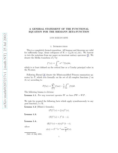
a rX iv:mat h /27237v1[mat h.NT]25J u l22A GENERAL STATEMENT OF THE FUNCTIONAL EQUATION FOR THE RIEMANN ZETA-FUNCTION LUISB ´AEZ-DUARTE 1.Introduction This is a completely formal exposition.All lemmas and theorems are valid for sufficiently large,dense subspaces of H :=L 2((0,∞),dx ).We borrow in toto the notations from my paper on invariant unitary operators [1].We denote the Mellin transform of f by f ∧(s ):= ∞0x s −1f (x )dx,which is at least defined on the critical line as a Cauchy principal value in the H -sense.Following Burnol [3]denote the M¨u ntz-modified Poisson summation op-erator by P ,which acts formally on the set of all complex functions f on (0,∞)according to P f (x ):=∞ n =1f (nx )−12Γ(s ).2LUIS B´AEZ-DUARTE2.General statements of the functional equationWe recall Theorem2.1of[1]:Theorem2.1.For any skew root T,and any real-valued generator g there is a unique,bounded,invariant operator W=W(T,g)with W g=T g.W is unitary and satisfies(T W)2=(W T)2=I,W−1=T W T.Why call the following triviality a“theorem”is a question left to the reader.Do note that the operator W depends explicitly on f.Theorem2.2(Main identity).Let f be good and suppose that P f is a real valued generator.Let T be a skew root and W=W(T,P f).ThenT P f=P W f.e Theorem2.1and the commutativity Lemma1.1.We specialize the main identity to give two general statements of the functional equation of the Riemann zeta function.Theorem2.3(Functional equation I).Let f be good and suppose that P f is a real valued generator.Let W=W(S,P f)and h=W f.Thenζ(1−s)f∧(1−s)=ζ(s)h∧(s).(2.1)Proof.The main identity is now SP f=P h,where we apply the Mellin transform using Lemmas1.2,1.3.Theorem2.4(Functional equation II).Let f be good and suppose that P f is a real valued generator.Let W=W(C,P f)and h=W f.Thenζ(1−s)φ(s)f∧(1−s)=ζ(s)h∧(s).(2.2)Proof.The main identity is now C P f=P h,where we apply the Mellin transform using Lemmas1.2,1.4.For an application of Theorem2.3choose f=χ,then P f(x)=−ρ(1/x) and W=U,so thath(x)=sin(2πx)s ,h∧(s)=−21−sπ−s cosπs1−s =−21−sπs cosπsZETA FUNCTIONAL EQUATION3 I don’t yet have a genuine application of Theorem2.4.However let as usual M(x):= n≤xµ(n),and choosef(x):=M(1/x).I have shown in[2]that this f∈H;on the other hand note that P f=χ. So again W=W(C,P f)=W(C,χ)=U.If one blithely insists on applying the theorem one obtains an intriguing equation from(2.2).Remark2.1.Quite frankly I am chagrined that I have not been included other genuine examples.More important perhaps is this question:how does this relate to Burnol’s view of the functional equation in[3]?References1.Luis B´a ez-Duarte,A class of invariant unitary operators,Advances in Mathematics,144,No.1(1999),1-12.2.Luis B´a ez-Duarte,Arithmetical versions of the Nyman-Beurling criterion for the Rie-mann hypothesis,Preprint2001,to appear as New versions of the Nyman-Beurling criterion for the Riemann Hypothesis to appear in IJMMS2002.3.Jean-Fran¸c ois Burnol,Co-Poisson intertwining:distribution and function theoreticaspects,preprint,15May2002.Luis B´a ez-DuarteDepartamento de Matem´a ticasInstituto Venezolano de Investigaciones Cient´ıficasApartado21827,Caracas1020-AVenezuelalbaezd@。
Conformal Field Theory Techniques in Large N Yang-Mills Theory

arXiv:hep-th/9311130v1 22 Nov 1993
Michael R. Douglas Dept. of Physics and Astronomy Rutgers University
1
Introduction
The first part of this article is an introduction to what might be called “large N representation theory,” Lie group representation theory with the focus on the limit N → ∞ of SU (N ) and the other classical groups. This has many applications in physics and mathematics, and good mathematical introductions exist, which tie it to its applications in group theory, soliton theory, combinatorics, and so forth. (See [1], 5.4 for a treatment very much like the one here; see also [2]) Now although it might seem that this theory would be invaluable for studying the large N limit of models with SU (N ) symmetry, and some examples in the physics literature are in [3], it does not get as much use as one might expect. Whether this isБайду номын сангаасsimply because the language is taking time to standardize,
Zeta functions with Dirichlet and Neumann boundary conditions for exterior domains
c h a o -d y n /9602005 3 Fe b 1996Zeta Functions with Dirichlet and NeumannBoundary Conditions for Exterior DomainsJ.-P.Eckmannand C.-A.Pillet 1D´e pt.de Physique Th´e orique,Universit´e de Gen`e ve,CH-1211Gen`e ve 4,Switzerland 2Section de Math´e matiques,Universit´e de Gen`e ve,CH-1211Gen`e ve 4,SwitzerlandWe generalize earlier studies on the Laplacian for a bounded open domain2with connected complement and piecewise smooth boundary.We compare it with the quantum mechanical scattering operator for the exterior of this same ing single layer and double layer potentials we can prove a number of new relations which hold when one chooses independently Dirichlet or Neumann boundary conditions for the interior and exterior problem.This relation is provided by a very simple set of -functions,which involve the single and double layer potentials.We also provide Krein spectral formulas for all the cases considered and give a numerical algorithm to compute the -function.1.IntroductionIn an earlier paper[EP2],we derived an identity between the integrated density of states for the eigenvalues for the Laplacian in a domain with Dirichlet boundary conditions,and the scattering phases for the exterior of the same domain,also with Dirichlet boundary conditions. In the present paper,we derive similar identities,and prove several of them,for the case where the boundary conditions can also be of Neumann type.We will discuss and illustrate similarities and differences between the various cases.Although it is not possible to really formulate the identities we are going to derive without making precise definitions,we summarize here the main results in an informal way.We consider a bounded domain in,and we let be its boundary.We denote by the free Green’s function.This is an analytic function of,except for a logarithmic singularity at the origin.We assume that the branch cut is along.We let,with ,denote the integral kernel of.Then we definewhere the normal points out of and is the restriction to the boundary.This is a more precise notation for the“normal derivative on the boundary.”Setting,we define4 -functions,for,The symbols and stand for Dirichlet and Neumann boundary conditions.Then we have the following nice identities between the integrated densities of states for the in the interior and the scattering phases for the exterior of,with boundary conditions ,Furthermore,We also have a Krein trace formula,valid for any nice function:where the are the eigenvalues of,the Laplacian in with boundary conditions. The S-matrix with boundary condition can also be described purely in terms of, ,or.We also give identities for the interacting Green’s functions in2cases:Here is the restriction to,and is the normal derivative on.Note that one of the consequences of Eq.(1.4)is a pointwise spectral duality,see Theorem3.3below.Finally,we describe an algorithm for computing the-function which is based on the double layer potential .This paper can be read in two ways.On the one hand,it can be viewed as a collection of identities relating Dirichlet,and Neumann scattering to Dirichlet and Neumann membranes in terms of single and double layer potentials on the boundary of,through certain-functions. Many of these identities,although reminiscent of work by[KR,HS,SU,BS2]are in fact new.On the other hand,we give detailed proofs for those identities involving the double layer potential,and relating Dirichlet conditions on one side of the boundary to Neumann conditions on the other.Acknowledgments.Our interest in the problems discussed in this paper has been provoked by the papers of Smilansky et al.[SU]and Steiner et al.[BS2].Part of ourfindings are a direct consequence of fruitful discussions with and inspiring seminars by members of these groups. In addition,we have profited from helpful discussions with V.Ivrii,A.Jensen,V.S.Buslaev and D.R.Yafaev.They all have contributed to clarify our views about the relevant issues.This work was supported by the Fonds National Suisse,and many of our contacts have been made possible by the semester“Chaos et quantification”at the Centre Emile Borel in Paris.2.Notations and DefinitionsWe consider domains which we call“standard domains.”Definition.A domain is called a standard domain ifa)is bounded.b)is piecewise,with afinite number of pieces.c)The angles at the corners are non-degenerate,i.e.,neither0nor.d)The complement of is connected.Remarks.–It should be noted that the definition allows for domains which consist of several pieces.We shall,however only deal with the case of a connected domain to keep the notation simple.–The theory would be somewhat easier,with bounds which are not really any better,if we restricted our attention to smooth domains.However,in view of applications and examples, we think that the inclusion of corners is important.To formulate our results,we need to define the various spectral densities and scattering phase shifts.Notation.We shall use throughout the subscripts and to denote Dirichlet and Neumann boundary conditions,respectively.We denote by a choice of boundary conditions among .Definitions.We define here the quantities,.Let be boundary conditions in .–The quantity denotes the number of eigenvalues below,counted with multiplicity, of.Here,is the Laplacian in with boundary condition on.–The quantity is the total scattering phase for the scattering operator in,with boundary conditions on.I.e.,.It is normalized to, and it is defined as a continuous function of.Our analysis will be based on a study of the single and double layer potentials which we define next.We denote by the Green’s functionand the integral kernel which goes with it:These are,respectively,the Hankel and Bessel functions(in the notations of[AS]).Note that is the free Green’s function,and the interaction will be described purely in terms of the boundary layer operators.Furthermore,the precise form of these functions is not relevant for our purpose,it suffices to know their asymptotic behavior for large and small arguments.Since we assume that the domain is connected,we can parameterize the boundary by arclength,by a map mapping into.Here,we assume without loss of generality that the length of is.We start by defining the“restrictions to the boundary.”Let be a function on.ThenHere,denotes the outward normal to at and indicates whether the limit is to be taken(along the normal)from the outside of()or the inside().Whenever the direction of the limit is irrelevant,we omit the index.In the corners,this definition is problematic, but since we only look at integral kernels,this does not matter.The following identities show where the various restrictions are defined:It is well known[Ne]that for allfrom which the appropriate domains of and can be read off.The notation is as follows: Let,where is the derivative with respect to arclength on.Then,for,is the subspace of functions with compact support,and denotes functions which are locally in,see[H].We also define.We next define the Single Layer Potential and the Double Layer Potential.For ,we haveThe notation means the gradient with respect to the second variable of.(The-dependence of is implicit.)A more suggestive notation isSince maps to for all,we see thatfor allHenceforth,we will omit the parentheses around.It is a well-known fact that the jump discontinuity of the single and double layer potential is1:More precisely,we have the relationThe operators,,and are defined as maps between the following spaces:For,this was shown in[EP1],for we will show it below,and for it will be a consequence of the bounds on and.The following expressions for the integral kernels may make explicit calculations more readable[CH]:where is the gradient with respect to the variable.The operator is the transpose of .The case of is more complicated and will be handled in the Appendix.Finally,we define the main objects of this paper,namely-functions,one for each of the boundary operators.Definition.We define4-functions.We choose some negative number and define,for :Thefirst index will refer to the interior boundary condition and the second to the exterior boundary condition.Remark.There is a close relationship among the4-functions,which is a consequence of the identity:The identity Eq.(2.7)follows from the following considerations:Fix and define the single layer potential.Then we have andandHence wefindfrom which thefirst identity in Eq.(2.7)follows.The second identity can be obtained by repeating the above arguments for in place of,i.e.,the limits are taken from the outside.Using the identity Eq.(2.7),it is almost obvious that it suffices to study the-functions ,,and.Then can be expressed asThis identity allows to avoid the use of which is more complicated to compute than or.3.The Relation Between the Scattering Phase and the Density of States Our main result is the following set of identities:Theorem3.1.For any choice of,the total scattering phases,the integrated density of states and the functions are related(for),byRemark.The relation Eq.(2.7)is reflected through the Eqs.(3.1),since the4possible left hand sides are linearly dependent.We furthermore have the bounds:Theorem3.2.One has the following bounds,valid for:Remark.With slightly more complicated expressions due to threshold effects the formulas above extend to.Discussion.The above results describe a close relation between the integrated density of states and total scattering phase.Thus,they are much weaker than the spectral duality result(“inside-outside duality”),conjectured in[DS]and proved in[EP1],but they generalize and extend the pioneering result of[JK].To complete the picture,we state here the result which relates individual eigenvalues and eigenphases:Theorem3.3.If is a standard domain,then is an eigenvalue of of multiplicityif and only eigenphases of the S-matrix in with Dirichlet boundary conditions approach from below as.If is a standard domain,then is an eigenvalue of of multiplicity if and only eigenphases of the S-matrix in with Neumann boundary conditions approach from above as.Remark.Thefirst part was shown in[EP1],the second part is new.We do not expect any similar result for the case when the boundary condition for the inside and the outside problem are not the same.Our convention of scattering phase is that the eigenphases of the(unitary) S-matrix are,.Remark.We next wish to comment on the bounds in Theorem3.2and their possible optimality. The growth of,has,in our view,two different origins in the case of and when compared to the“mixed”cases and.In the case of the growth can be traced back to the different Weyl asymptotics of and[SU],namelywhere the superscript indicates the Weyl approximation,so that already at the“average”level the two quantities differ by.A similar formula holds for the pure Neumann case.On the other hand,in the case of,there is a different asymptotics sinceand therefore there is a cancellation of the terms of order at the Weyl level.We next discuss in detail the question whether this cancellation implies better bounds in Eqs.(3.3)and(3.4).(We neglect here the issue of eliminating the factor.) Afirst possibility might seem a proof using the properties of.Indeed,in the integral kernel of there appears the product which goes to0as ,so that in the detailed bounds one additional order cancels when compared to the boundon,which occurs in the estimate for(see Eq.(5.10)).However,we still cannot exclude that the bounds in Eqs.(3.3)and(3.4)are optimal,since actually the cancellation does not take place at intermediate distances,i.e.,.A second possibility is provided by the very detailed results from the methods of pseudo-differential operators.The following discussion is a summary of the papers by Seeley,Melrose, Ivrii,Buslaev,Robert,and Vasil’ev,Safarov[VS].The major new ingredient here is the notion of the set of periodic orbits of same length.We say that a billiard has property S(for synchronous) if there are“many”periodic orbits in the following sense.Consider a periodic orbit,of period .Let denote the phase space point reached from(initial position and initial direction of the orbit)after time,i.e.,the end point of the billiard trajectory(in phase space)with initial time.Let be the periodic point:.We say this orbit is“absolutelyperiodic”[VS]ifhas a zero of infinite order at.In other words,the returning rays have infinite focusingin a neighborhood of.A billiard has property S if the set of absolutely periodic points haspositive measure in phase space.(For example,if is a“devil’s staircase,”then it has a set offull measure of points where vanishes of infinite order when.)Examples of billiards with property S are given in[VS].If a billiard does not have property S,we saythat it has property A(for asynchronous).When talking about scattering,this condition is to beapplied to exterior orbits,which might for example be trapped in the“outside”of an obstacle.Ifa billiard has property S,the term of order in the Weyl series is modified by an oscillatingamplitude,,which can in principle be computed from the knowledge of the synchronousset.If is convex and the boundary is an analytic curve,then one has property A,but in mostother cases,it is difficult to decide whether a domain has property A or S.The following tablesummarizes the known results for boundary(in dimension2,in odd dimensions,slightlymore is known).The upper sign is for Dirichlet,the lower for Neumann boundary conditions.PropertyS4.The Krein FormulaUsing the methods of[EP2],one can derive from the identities of Theorem3.1a corresponding set of Krein trace formulas and,in the case of identical boundary conditions only,a Green’s formula.We shall state them here without proof.Definition.We let,and we define the“interacting”Hamiltonians Furthermore,we denote by the eigenvalues(counted with multiplicity)of,and by the on-shell S-matrix for scattering on,with boundary conditions.With these notations,one has theTheorem4.1.For every choice of and for all with support in ,one has the identity.If we denote by the energy surface,,then we see that for all,Theorem4.2.The S-matrix at energy can be expressed as follows:Note that and all the other combinations of and used above are well-defined.Wefinally state two identities between Green’s functions.Note that no such identity is available in the case when the inside boundary condition is not the same as the outside boundarycondition.Theorem4.3.The Green’s functions satisfy the following identities:The boundary layer integral lends itself in a very natural and systematic way for the computation of,as well as for a determination of the eigenvalues and,to some extent ofthe scattering phases for the Dirichlet,resp.the Neumann problem.These algorithms work,at present,only for the case of domains where is,i.e.,corners are excluded,but jumps inthe second derivative are allowed.Consider the integral kernel.To discretize it,we choose an ordered sequence of points on the boundary(this method is also used in[HS]).Ifthe boundary is smooth,it is advisable to choose the points equidistant in arclength,since then the method is of infinite order in the step size[Ha].In the other cases,we have chosen unequal steps,and in particular2points at distance0at every discontinuity of the second derivative of the boundary,one point as the limit on either side.5.Bounds on the Double Layer PotentialOur main ingredient for the proof of all the results stated so far are Structure Theorems,which describe the detailed regularity properties of the operators and,and hence,by Eq.(2.7), also those of.Wefirst state this result:Definitions.If is a compact operator,we let,denote the eigenvalues of in decreasing order.One defines the weak Schatten classes(for),as the set of those for whichisfinite.We also define the associated normsWe let denote the orthogonal projection onto the constant functions in.Recall also that.Definitions.We need some precisions concerning the branch cuts in the definition of, cf.Eq.(2.1).Let denote,and let denote the Riemann surface associated with the logarithm.The function is defined on,and the integral kernel is defined for,with the convention that for.Then we haveStructure Theorem5.1.–For the operator has the following representation:,where is Hilbert-Schmidt,and where is trace class.Moreover,there is a constant so that for,one has the boundsThe operators and do not depend on.–For the operator has the following representation:where is bounded and of normseems to be absent from ,it reappears naturally through the very definition of,Eqs.(2.2)and(2.3).So the results for and are in fact quite similar.In particular,as discussed before,we do not get better results for than for,although such a result might have been expected from a local analysis.Proof.The proofs for the operators have been given in[EP2],[EP1],so we deal here only with.We notefirst that the Green’s function equals,where is the Hankel function,cf.[AS,9.1],For(which is really a complex energy)we let.Starting from Eq.(2.5),we see that the integral kernel for iswherewithThe local behavior of is given bycf.[AS,9.1].We will also need in the sequel the representation With these notations,we define the regular and singular parts of: so that.Note that does not depend on.Proposition5.2.The operator is in the Schatten class2/3and for all one has the boundProof.In order to bound,we consider the quantity.From Eq.(5.6),we get the representationFurthermore,we have,with,We have used here that implies.In the complement,we use that the integrand is bounded by,and a scaling argument shows that, as.The proof of Eq.(5.8)is complete.Proof of Proposition5.2.Notefirst thatwhere is unitary.Therefore,the Schwarz inequality and Eqs.(5.8),(5.9),implySince the spectrum of is,and is Hilbert-Schmidt.Proof of the Structure Theorem5.1.This is an immediate consequence of Proposition5.4and Proposition5.2and an inequality of the type of Eq.(5.11).Remark.We shall use the notation to denote equality modulo Hilbert-Schmidt operators, i.e.,means that is Hilbert-Schmidt.Proof of Proposition5.4.We shall localize the integral kernel of near the corners and in the complement of this region,and give a different treatment for the two pieces.To localize, assume the boundary has exactly corners,and define smooth functionswhich are equal to1when are both close to the corner,and such that they have disjoint supports.We then further decompose into the functionswhere is1if are on opposite sides of(and close to)corner,and0otherwise,and .We next describe the local behavior of on a smooth part of and near a corner of.Lemma5.5.On the smooth pieces of one hasFrom this and the compactness of it follows that the corresponding contribution of is Hilbert-Schmidt.Proof of Lemma5.5.We recall the definition of:Since we consider the smooth part of,we get,with denoting the tangent vector, Substituting in Eq.(5.13),the assertion Lemma5.5follows.We next study the behavior“across”one corner,i.e.,.Lemma5.6.Modulo Hilbert-Schmidt operators,the operators are bounded in norm by,where is the interior angle at the corner.Since the havedisjoint supports,it follows that there is a Hilbert-Schmidt operator(which is independent of the energy),for which one has the inequalityProof.We assume that the boundary is locally straight.We leave to the reader the study of the Hilbert-Schmidt correction terms generated by curvature near a corner,see[EP1].Assume for convenience that the corner is at the origin and use coordinates and near the corner, when and.:The local coordinate system.Elementary geometry leads toRedoing this calculation for,,wefind that for all,satisfying one has We shall consider near one corner.Wefind,that equals(locally)The operator is diagonalized by the Mellin transformation,defined byas we shall show now.Indeed,this is intuitively clear since diagonalizes dilatations.Notethat is unitary.With the above notation,we see that is given by Thus,becomes matrix multiplication under the Mellin transform.We next evaluate theintegral.Note that the integrand is at infinity and near0.Therefore, for large,wefindNote that when.We next observe that on the space,we have:The contour used in evaluating the integral()of Eq.(5.15).From this it follows at once that the spectrum of the corner contribution isThis set is shown in Fig.3,for various values of as a function of.It is easy to check that the set is contained in the disk of radius-0.4-0.20.20.4Re-0.4-0.20.20.4Im :The functions ()for angles20,119.AppendixThe definition and explicit study of the operator are more complicated than those of given in [EP1]and those of given in Section 5.These additional difficulties are generated by the appearance of two derivatives in the definition of ,which make it an operator of order 1.However,when considering the integral kernel of ,important cancellations of singularities take place,even in the presence of corners ,and the main purpose of this appendix is a sketch of the mechanisms implying these calculations.Detailed notes on this problem can be requested from the authors.We fix first some simple notations.If ,,then we denoteThe sums above are over the corners ,which are located at,whereand with a similar definition for .The operator is defined starting from the double layerpotential ,which we defined for byThenfor all except the corners.It is not really obvious that the above limit exists,but we shall give a few arguments on the way to proving this.We want to argue only modulo Hilbert-Schmidt operators and we use the sign to denote equality modulo Hilbert-Schmidt operators(with bounds independent of the energy).We notefirst the identity,with ,,.In the limit process,the arguments of and will be ,and then wefind that(modulo Hilbert-Schmidt,as announced)where is the derivative of.This result also allows us to compare to.In particular,it means thatand therefore,by the Structure Theorem II of[EP2],we see that for all,,is Hilbert-Schmidt and is trace class.Note that does not depend on and that is actually in the Schatten class.Of course,these facts also follow from the identity Eq.(2.7)and from the(explicitly proved)facts about,[EP2,Structure Theorem II] and,Structure Theorem5.1.References[AS]Abramowitz,M.and I.Stegun:Handbook of Mathematical Functions,New York,Dover(1965).[BS]Birman,M.Sh.and M.Z.Solomyak:Spectral Theory of Selfadjoint Operators in Hilbert Space,Dordrecht, Reidel(1987).[BS2]Burmeister,B.and F.Steiner:(To appear).[CH]Courant,R.and D.Hilbert:Methods of Mathematical Physics,Vol.1,New York,J.Wiley(1953). [DS]Doron,E.and U.Smilansky:Semiclassical quantization of billiards—a scattering approach.Nonlinearity 1055–1084(1992).[EP1]Eckmann,J.-P.and C.A.Pillet:Spectral duality for planar mun.Math.Phys.,283–313 (1995).[EP2]Eckmann,J.-P.and C.A.Pillet:Scattering phases and density of states for exterior domains.Ann.Inst.Henri Poincar´e,383–399(1995).[Ha]Hairer,E.:(Private communication).[He]Hesse,T.:Trace formula for a non-convex billiard system.Preprint.[HS]Harayama,T.and A.Shudo:Zeta function derived from the boundary element method.Physics Lett.,417–426(1992).[H]H¨o rmander,L.:The Analysis of Linear Partial Differential Equations,Berlin,Heidelberg,New York,Springer(1983–1985).[JK]Jensen,A.and T.Kato:Asymptotic behaviour of the scattering phase for exterior m.Part.Diff.Equ.,1165–1195(1978).[KR]Kleinman,R.E.and G.F.Roach:Boundary integral equations for the three-dimensional Helmholtz equa-tion.SIAM Review,214–236(1974).[N]Neˇc as,J.:Les M´e thodes Directes en Th´e orie des Equations Elliptiques,Paris:Masson(1967).[R1]Robert,D.:Sur la formule de Weyl pour des ouverts non born´e s.C.R.Acad.Sci.Paris,29–34 (1994).[R2]Robert,D.:A trace formula for obstacles problems and applications.In Mathematical Results in Quan-tum Mechanics.International Conference in Blossin(Germany),May17–21,1993.Series:Operator The-ory:Advances and Applications,(Demuth,M.,Exner,P.,Neidhardt,H.,Zagrebnov,V.eds.).Basel, Boston,Berlin,Birkh¨a user(1994).[SU]Smilansky,U.and sishkin:The smooth spectral counting function and the total phase shift for quan-tum billiards.J.Physics A(in print).[VS]Vasil’ev,D.G.and Yu.G.Safarov:The asymptotic distribution of eigenvalues of differential operators.Amer.Math.Soc.Transl.(2),55–110(1992).。
ON THE DISTRIBUTION OF SPACINGS BETWEENZEROS OF THE ZETA FUNCTION
log T + α + o ( 1 ) as T → ∞ ,
(1.2)
uniformly for 0 ≤ α ≤ 1. Montgomery also presented heuristic arguments which suggested that F ( α , T ) = 1 + o ( 1 ) as T → ∞ (1.3)
-3-
to be distributed like a Poisson random variable [29]. The conjecture (1.4) suggests some further topics for investigation. In the language of mathematical physics, this conjecture says that 1 − ( ( sin π u ) / ( π u ) ) 2 is the pair correlation function of zeros of the zeta function. F. J. Dyson pointed out [56] that the gaussian unitary ensemble (GUE) has the same pair correlation function. The GUE has been studied very extensively in mathematical physics together with the gaussian orthogonal ensemble (GOE) and the gaussian symplectic ensemble (GSE) as models for distribution of energy levels in many-particle systems. The GUE consists of n × n complex hermitian matrices of the form A = ( a j k ), where a jj = 2 1 / 2 σ j , j , _ a j k = σ j , k + i η j , k for j < k, and a j , k = a k , j = σ k , j − i η k , j for j > k, where the σ j , k and η j , k are independent standard normal variables. When n → ∞ and the eigenvalues of the matrices of the GUE are suitably normalized, their pair correlations becomes 1 − ( ( sin π u ) / ( π u ) ) 2 . (The pair correlations of the GOE and GSE are different.) For more information about the GUE and the other ensembles, the reader is referred to [2, 4, 11, 41, 54, 59, 63]. The possible connection between zeros of the zeta function and eigenvalues of random matrices is of interest in number theory because of the Hilbert and Po ´lya conjectures [56, 59] which say that the zeros of the zeta function correspond to eigenvalues of a positive linear operator. If true, the Hilbert and Po ´lya conjectures would imply the RH, and some people feel that the most promising way to prove the RH is by finding the right operator and establishing the necessary results about it. One can argue heuristically that if such an operator exists, its eigenvalues might behave like those of a random operator, which in turn might behave like the limit of a sequence of random
Noncommutative resolutions of ADE fibered Calabi-Yau threefolds
a rXiv:086.3177v1[mat h.A G]19J u n28NONCOMMUTATIVE RESOLUTIONS OF ADE FIBERED CALABI-YAU THREEFOLDS ALEXANDER QUINTERO V ´ELEZ AND ALEX BOER A BSTRACT .In this paper we construct noncommutative resolutions of ADE fibered Calabi-Yau threefolds.The construction is in terms of a noncommu-tative algebra introduced by V .Ginzburg in [16],which we call the “N =1ADE quiver algebra”.I NTRODUCTION In recent years,there has been a great deal of interest in noncommutative algebra in connection with algebraic geometry,in particular to the study of sin-gularities and their resolutions.The underlying idea in this context is that the resolutions of a singularity are closely linked to the structure of a noncommuta-tive algebra.The case of Kleinian singularities X =C 2/G ,for G a finite subgroup of SL(2,C ),was the first non-trivial example of this phenomenom,studied in [10].It was shown that the minimal resolution of X can be described as a moduli space of representations of the preprojective algebra associated to the action of G .This preprojective algebra is known to be Morita equivalent to the skew group algebra C [x,y ]#G ,so we could alternatively use this algebra to construct the minimal resolution of X .Later,M.Kapranov and E.Vasserot [19]showed that there is a derived equivalence between C [x,y ]#G and the minimal resolution of X .A similar statement was established by T.Bridgeland,A.King and M.Reid [6]for crepant resolutions of quotient singularities X =C 3/G arising from a finite subgroup G ⊂SL(3,C ).In this case the crepant resolution of X is realized as a moduli space of representations of the McKay quiver associated to the action of G ,subject to a certain natural commutation relations (see [12]and§4.4of [16]).Various steps in the direction mentioned above have been taken in a series of papers [26,25,17,30,36],where several concrete examples have been dis-cussed.More abstract approaches have also been put forward in [24,4].The lesson to be drawn from these works is that for some singularities it is possible to find a noncommutative algebra A such that the representation theory of this2ALEXANDER QUINTERO V´ELEZ AND ALEX BOERalgebra dictates in every way the process of resolving these singularities.More precisely,it is shown that:•the centre of A corresponds to the coordinate ring of the singularity;•the algebra A isfinitely generated over its centre;•“nice”resolutions of the singularity are obtained via the moduli space of representations of A;•the category offinitely generated modules over A is derived equivalent to the category of coherent sheaves on an appropriate resolution. Following the terminology of M.Van den Bergh(cf.[34,35])we may think of A as a“noncommutative resolution”.This phenomenom also appears naturally in string theory in the context of coincident D-branes.There the singularity X should be a Calabi-Yau threefold and one studies Type IIB string theory compactified on X.It turns out that a collection of D-branes located at the singularity gives rise to a noncommu-tative algebra A,which can be described as the path algebra of a quiver with relations.For afixed quiver Q,this construction only depends on a‘noncommu-tative function’called the superpotential.As a consequence,the aforementioned derived equivalence establishes a correspondence between two different ways of describing a D-brane:as an object of the derived category of coherent sheaves on a resolution of X and as a representation of the quiver Q.Now,let us explain the situation on which we will focus.We shall study a kind of singular Calabi-Yau threefolds with isolated singularities,known as ADEfibered Calabi-Yau threefolds.They have been defined and studied in the work of F.Cachazo,S.Katz and C.Vafa[9]from the point of view of N=1 quiver gauge theories.The quiver diagrams of interest here are the extended Dynkin quivers of type A,D or E.Following[16],for such a quiver Q,we associate a noncommutative algebra Aτ(Q)which we call the“N=1ADE quiver algebra”.The choice ofτis encoded in thefibration data.The goal of this paper is to show that the N=1ADE quiver algebra realizes a noncommu-tative resolution of the ADEfibered Calabi-Yau threefold associated with Q and τ.The proof of this result depends on two ingredients.On the one hand,we use the results in[10],on the construction of deformations of Kleinian singularities and their simultaneous resolutions in terms of Q.On the other hand,we use the results in[15]to contruct a Morita equivalence between Aτ(Q)and a noncom-mutative crepant resolution Aτin the sense of Van den Bergh;this allows us to use the techniques developed in[34]to show that the derived category offinitely generated modules over Aτ(Q)is equivalent to the derived category of coherent sheaves on the small resolution of the ADEfibered Calabi-Yau threefold. Some related results using different methods were obtained by B.Szendr˝o i in[32].He considers threefolds Xfibered over a general curve C by ADE singularities and shows that D-branes on a small resolution of X are classified by representations with relations of a Kronheimer-Nakajima-type quiver in theNONCOMMUTATIVE RESOLUTIONS OF ADE FIBERED CALABI-YAU THREEFOLDS3category Coh(C)of coherent sheaves on C.The correspondence is given by a derived equivalence between the small resolution of X and a sheaf of non-commutative algebras on C.In particular,there is a substantial overlap between Section4of this paper and the results of Ref.[32].An effort has been made to make this paper as self-contained as possible.The paper is structured as follows.In Section1we will review the theory of de-formations of Kleinian singularities and their simultaneous resolutions and we define ADEfibered Calabi-Yau threefolds.In Section2we outline the results of Cassens and Slodowy on the construction of deformations of Kleinian singu-larities and their simultaneous resolutions in terms of Q.In Section3we define the N=1ADE quiver algebra Aτ(Q),describe some of its basic structure and prove that small resolutions of ADEfibered Calabi-Yau threefolds are obtained via the moduli space of representations of Aτ(Q).We conclude with a discus-sion of the derived equivalence between Aτ(Q)and the small resolution of an ADEfibered Calabi-Yau threefold in Section4.Acknowledgments.We would like to thank Bal´a zs Szendr˝o i for helpful remarks and e-mail correspondence.A.Q.V.is grateful to Jan Stienstra for his constant guidance and also for some essential conversations.A.Q.V.is also grateful to Tom Bridgeland and Michel Van den Bergh for valuable discussions related to this work. A.B.thanks A.Q.V.for introducing him to this problem.1.P RELIMINARIESIn this section we will briefly review the definition of ADEfibered Calabi-Yau threefolds,as developed in[9].We begin by outlining the theory of deformations of Kleinian singularities and their simultaneous resolutions.For more details on these topics,we refer the reader to[21],[23]and[18].1.1.Deformations of Kleinian singularities.We remind briefly the basic set-ting.Recall that Kleinian singularities are constructed as the quotient of C2by afinite subgroup G of SL(2,C).Suchfinite G are known to fall into an ADE classification:up to conjugacy,they are in one-to-one correspondence with the Dynkin diagrams of type A,D or E.The quotient C2/G can be realized as a hypersurface X0⊂C3with an isolated singularity at the origin.The defining equation for the singularity is determined by the Dynkin diagram associated to the group G:A n:x2+y2+z n+1=0D n:x2+y2z+z n−1=0E6:x2+y3+z4=0E7:x2+y3+yz3=0E6:x2+y3+z5=04ALEXANDER QUINTERO V´ELEZ AND ALEX BOERWriteπ:Y0→X0for the minimal resolution.The exceptional divisor ofπconsists of(−2)-curves C i intersecting transversally.This configuration is best explained via the dual graphΓof X0:each curve C i is a vertex,and two vertices are joined by an edge if and only if the corresponding curves intersect in Y0.For Kleinian singularities,the resolution graph is just a Dynkin diagram of type A, D or E.For this reason,this singularities are also called ADE singularities. The Dynkin diagram appears in the classification of simple Lie algebras.Thus we have a complex simple Lie algebra g corresponding toΓ.We let h be the complex Cartan subalgebra of g and W the corresponding Weyl group.On h, we have a natural action of W.For later use we briefly discuss the notion of semiuniversal deformation of a singularity.Let S be a complex space with a distinguished point s0.A deforma-tion of a complex space X0consists of aflat morphismϕ:X→S togetherwith an isomorphism X0∼=X s0=ϕ−1(s0).The space S is called the base ofthe deformationϕ.An isomorphism of two deformationsϕ:X→S andϕ′:X′→S of X0over S is an isomorphismθ:X→X′such that the following diagram commutesXθNONCOMMUTATIVE RESOLUTIONS OF ADE FIBERED CALABI-YAU THREEFOLDS5 Now we want to construct semiuniversal deformations of Kleinian singular-ities.From what we have discussed above,each Kleinian singularity has an associated Dynkin diagramΓwhose Weyl group W acts on the complex Cartan subalgebra h of the associated Lie algebra g.A model for the base of the defor-mation is given by S=h/W.The defining polynomial of X is simple to write in the A n and D n cases,namelyA n:x2+y2+z n+1+n+1 i=2αi z n+1−iD n:x2+y2z+z n−1−n−1i=1δ2i z n−1−i+2γn ywhereαi is the i th elementary symmetric function of t1,...,t n+1,δ2i is the i th elementary symmetric function of t21,...,t2n andγn=t1···t n.The correspond-ing equations for E6,E7and E8in terms of the t’s are more complicated and we refer the reader to[21].1.2.Simultaneous resolutions for Kleinian singularities.Kleinian singular-ities are exceptional among the other surface singularities because they admit simultaneous resolutions.We start by recalling the definition of a simultanoeus resolution.Letϕ:X→S be aflat morphism of complex spaces.A simultaneous resolution ofϕis a commutative diagramX′ϕ′X ϕSsuch thatϕ′:X′→T isflat,u isfinite and surjective,πis proper,and for allt∈T,the morphismπ|X′t :X′t→X u(t)is a resolution of singularities.If S is apoint,then a simultaneous resolution ofϕ:X→S is the same as a resolution of X.Brieskorn and Tyurina[7,33]showed that the semiuniversal deformationϕ: X→h/W,for any Kleinian singularity X0,admits a simultaneous resolution after making the base change h→h/W.More precisely,the family X×h/W h may be resolved explicitly and one obtain a simultaneous resolution Y→X×h/W h ofϕinducing the minimal resolution Y0→X0.The situation can be conveniently summarized by the diagramYh6ALEXANDER QUINTERO V ´ELEZ AND ALEX BOERWe should mention that there is a more general construction obtained from simultaneous partial resolutions of X 0;if we let Γ0⊂Γbe the subdiagram for the part of the singularity that is not being resolved and denote by W 0⊂W the subgroup generated by reflections of the simple roots corresponding to Γ\Γ0,then we can define a deformation of X 0,which has a model for the base given by h /W 0,and there is a simultaneous partial resolution Z of the family X ×h /W 0h .We will illustrate this with an example.Example 1.1.We consider a singularity of type A n .In the space C n +1with co-ordinates t 1,...,t n +1,there is a natural identification of h with the hyperplane given by the equation n+1i =1t i =0.The Weyl group W is isomorphic to thesymmetric group S n +1.The quotient map h →h /W can be realized by the formula αi =σi (t 1,...,t n +1),where σi is the i th elementary symmetric func-tion of t 1,...,t n +1.Making a finite base change h →h /W ,one gets a family X ×h /W h given in C 3×h by the equationx 2+y 2+n +1 i =1(z +t i )=0with discriminant locus i<j (t i −t j )2=0.This can be rewritten after an analytic coordinate change asxy =n +1 i =1(z +t i ).The resolution Y can be constructed explicitly as the clousure of the graph of the rational map X ×h /W h →(P 1)n defined by (x,y,z,t i )−→ j i =1(z +t i ):y .Let (u j :v j )be homogeneous coordinates on the j th P 1arising from the resolu-tion described above.Thenxy =n +1 i =1(z +t i )xv j =u jn +1 i =j +1(z +t i ),1≤j ≤n yu j =v jj i =1(z +t i ),1≤j ≤nu j v k =u k v jj i =k +1(z +t i ),1≤k <j ≤nNONCOMMUTATIVE RESOLUTIONS OF ADE FIBERED CALABI-YAU THREEFOLDS7 are the equations for Y.The projection C3×h×(P1)n→h induces a map ψ:Y→h,and the composition C3×h×(P1)n→C3×h→C3×h/W induces a mapπ:Y→X.By construction,the following diagram is commutative:Y ψXϕh/WWe claim that this diagram is a simultaneous resolution ofϕ.Let U0,U1,...,U n be the open subsets of C3×h×(P1)n defined byU0={v1=0},U k={u k=0,v k+1=0},1≤k≤n−1U n={u n=0},and on U k,letξk=v k/u k,ηk=u k+1/v k+1.In Y∩U k we can solve for the(u j:v j),j=k,k+1,by(u j:v j)= 1:ξk k i=j+1(z+t i) ,for j<k(u j:v j)= ηk j i=k+2(z+t i):1 ,for j>k+1.An elementary computation shows that Y∩U k may be defined by the above equations together with the equationsx=ηk n+1 i=k+2(z+t i),y=ξkk i=1(z+t i),z=ξkηk−t k+1.Consequently,it may be inferred that Y is non-singular,andψhas maximal rank,whenceψisflat.It is now routine to verify that the diagram above is a simultaneous resolution ofϕ.1.3.ADEfibered Calabi-Yau threefolds.We now describe a certain class of Calabi-Yau threefolds constructed in[9]by F.Cachazo,S.Katz and C.Vafa(see also[8,20,31,37]).8ALEXANDER QUINTERO V´ELEZ AND ALEX BOERWe begin with some preliminaries.By a Gorenstein Calabi-Yau threefold X we always mean a quasiprojective threefold X with only terminal Gorentein sin-gularities such that K X=0.Fix a Gorenstein Calabi-Yau threefold X.A small resolutionπ:Z→X is a proper birational morphism from a normal variety Z to X such that the expectional locus is a curve.We are mainly interested in the case where P∈X is an isolated Gorenstein threefold singularity.In this case C=π−1(P)is a disjoint union of smooth rational(−1,−1)-curves C i.We point out the following important result,originally due to M.Reid(cf.[28]). Proposition1.2.Let P∈X be an isolated Gorenstein threefold singularity andπ:Z→X a small resolution.Then the generic hyperplane section X0 through P is a Kleinian singularity,and its proper transform Z0on Z has iso-lated singularities,hence is normal,and is dominated by the minimal resolution of X0.In light of this result,we can locally view X as the total space of a one parame-ter family of deformations of its generic hyperplane X0,and the small resolution Z as the total space of a one parameter family of deformations of a partial reso-lution Z0of X0.We are thus in the presence of the phenomenon of simultaneous partial resolutions of Kleinian singularities.Using these observations we can define a broader class of Calabi-Yau three-folds as follows.We want to obtain a Gorenstein Calabi-Yau threefold X by fibering the total space of the semiuniversal deformation of a Kleinian singular-ity X0over a complex plane whose coordinate we denote byλ.Thisfibration is implemented by allowing the t i’s to be polynomials inλ.In more concrete terms,let f:C→h be a polynomial map1.Via the defining equation for the family X×h/W h,we can view X as the total space of a one parameter family defined by f.Similarly,the simultaneous resolution Y→X×h/W h can be used to construct a Calabi-Yau threefold Y.That is,we get a cartesian diagramY YfC1More general and more local constructions can be obtained from polynomial maps f:∆→h with∆a complex disk,but we choose C as the domain of f for application to physics.NONCOMMUTATIVE RESOLUTIONS OF ADE FIBERED CALABI-YAU THREEFOLDS9 to each positive rootρof h.This class of Calabi-Yau threefolds we call ADE fibered Calabi-Yau threefolds.Note that if f=0,then the singular threefold X is isomorphic to a direct product of the form X0×C.In particular X has a line of Kleinian singularities. The resolution Y is isomorphic to the direct product Y0×C,where Y0is the minimal resolution of X0.This of course is not a small resolution,as it has an exceptional divisor over a curve.The main point for us here is that ADEfibered Calabi-Yau threefolds are related to X0×C by a complex structure deformation. For a full discussion of these matters consult[31,32].We illustrate with the following example.Example1.3.Let P∈X be an isolated A n singularity.We keep the notation of Example1.1.A polynomial map f=(t1,...,t n+1):C→h would give the t i’s as polynomial functions ofλ.The singular threefold X can be induced from X×h/W h by the morphism f.In other words,X is given by(x,y,z,λ) xy=n+1 i=1(z+t i(λ)) ⊂C4.Y is the resolution of the above given by taking the closure of the graph of the mapping X→(P1)n given by(u j:v j)= j i=1(z+t i(λ)):y ,1≤j≤n.As with Example1.1we define n+1open subsets on C4×(P1)n as follows: U0={v1=0},U k={u k=0,v k+1=0},1≤k≤n−1U n={u n=0}.Settingξk=v k/u k,ηk=u k+1/v k+1for1≤k≤n−1and observing that Y⊂C4×(P1)n satisfiesxv j=u j n+1i=j+1(z+t i(λ)),1≤j≤nyu j=v jji=1(z+t i(λ)),1≤j≤nu j v k=u k v jji=k+1(z+t i(λ)),1≤k<j≤n10ALEXANDER QUINTERO V´ELEZ AND ALEX BOERone can solve for the(u j:v j),j=k,k+1,by(u j:v j)= 1:ξk k i=j+1(z+t i(λ)) ,for j<k(u j:v j)= ηk j i=k+2(z+t i(λ)):1 ,for j>k+1.It follows that Y is obtained by glueing n+1copies of C3with coordinates (ξk,ηk,λ)and transition mapsξk+1=ξ−1k,ηk+1=ηk(ξkηk−t k+1(λ)),λ=λ.The contraction mapπ:Y→X is defined on U k byx=ηk n+1i=k+2(z+t i(λ)),y=ξkki=1(z+t i(λ)),z=ξkηk−t k+1(λ),which extends over the whole of Y.2.D EFORMATIONS AND SIMULTANOEUS RESOLUTIONS OF K LEINIANSINGULARITIES REVISITEDA new approach to the deformation and resolution theory of Kleinian singu-larities was given by H.Cassens and P.Slodowy[10].Their construction starts directly from the McKay graph of thefinite subgroup G of SL(2,C)and uses geometric invariant theory.In this section,we describe some aspects of this construction we shall need in the sequel.2.1.Quivers.First of all,let us briefly remind the definitions and the basic properties of quivers and their representations.Recall that a quiver Q=(Q0,Q1,h,t)consists of afinite set Q0of vertices,a finite set Q1of arrows and two maps h,t:Q1→Q0which assign to each arrow a∈Q1its head h(a)and tail t(a),respectively.We shall write a:i→j for an arrow starting in i and ending in j.A path in Q of length m≥0is a sequence p=a1a2···a m of arrows such that t(a i+1)=h(a i)for1≤i≤m−1.We let h(p)=h(a m)and t(p)=t(a1) denote the initial andfinal vertices of the path p.For each vertex i∈Q0,we let e i denote the trivial path of length zero which starts and ends at the vertex i.The path algebra C Q associated to a quiver Q is the C-algebra whose underlying vector space has basis the set of paths in Q,and with the product of paths givenby concatenation.Thus,if p=a1···a m and q=b1···b n are two paths,then pq=a1···a m b1···b n if t(q)=h(p)and pq=0otherwise.We also have,e i e j= e i if i=j0if i=j,e i p= p if t(p)=i0if t(p)=ipe i= p if h(p)=i,0if h(p)=ifor p∈C Q.This multiplication is associative.Note that i∈Q0e i is the identity element of C Q.We denote by mod–C Q the category offinitely generated right modules over C Q.The path algebra C Q is sometimes too big to be of interest and so often instead we wish to consider the path algebra modulo an ideal.This ideal is often defined by using relations on the quiver.Formally,a relationσon a quiver Q is a C-linear combination of pathsσ=c1p1+···+c n p n with c i∈C and h(p1)=···=h(p n)and t(p1)=···=t(p n).Ifρ={σr}is a set of relations on Q, the pair(Q,ρ)is called a quiver with relations.Associated with(Q,ρ)is the C-algebra A=C Q/(ρ),where(ρ)denotes the ideal in C Q generated by the set of relationsρ.A representation V of Q is a collection{V i|i∈Q0}offinite dimensional vector spaces over C together with a collection{V a:V t(a)→V h(a)|a∈Q1}of C-linear maps.The dimension vector of the representation V is the vector dimFor a dimension vectorα∈Z Q0we define the representation spaceRep(Q,α)= a∈Q1Hom C(Cαt(a),Cαh(a))which is an irreducible variety of dimension a∈Q1αt(a)αh(a).Given a point x∈Rep(Q,α),we define a representation V(x)of Q of dimension vectorαby declaring that V(x)i=Cαi and that V(x)a is the C-linear map x a.There is a canonical action of the linear reductive group GL(α)= i∈Q0GL(αi,C)on the representation space Rep(Q,α)determined for all elements x∈Rep(Q,α)of GL(α)by the ruleand all group elements g=(g i)i∈Q.(g·x)a=g h(a)x a g−1t(a)It is clear that the closed orbits of GL(α)on Rep(Q,α)are precisely the isomor-phism classes of representations.Ifρis a set of relations for Q,we denote by Rep(A,α)the closed subspace of Rep(Q,α)corresponding to representations for A=C Q/(ρ).As before,we can see that the closed orbits of GL(α)on Rep(A,α)correspond to isomorphism classes of representations of A of dimen-sionα.Of these,the orbits on which GL(α)acts freely are those corresponding to a simple representation of A.2.2.Deformation of Kleinian singularities revisited.This subsection is de-voted to constructing the semiuniversal deformation of a Kleinian singularity in terms of the associated quiver.We follow the general approach described in Ref.[15](see also[13]and[14]).We begin by defining the deformed preprojective algebra.Let Q be a quiver with vertex set I.We denote byQ a∈Q[a,a∗]− i∈Iτi e i .where[a,a∗]is the commutator aa∗−a∗a.The algebraΠ(Q)=Π0(Q)is known as the preprojective algebra.The representations ofQ,α)=Rep(Q,α)⊕Rep(Q op,α),where Q op is the opposite quiver to Q with an arrow a∗:j→i for each arrow a:i→j in Q.As earlier,we have a natural action of the reductive group GL(α)= i∈I GL(αi,C)on Rep(corresponding to arrows a and a∗,also Rep(Q op,α)∼=Rep(Q,α)∗.Thus,there is an identification of the cotangent bundle T∗Rep(Q,α)of Rep(Q,α)with Rep(Q,α)∼=Rep(Q,α)×Rep(Q,α)∗=T∗Rep(Q,α).The natural symplectic form on T∗Rep(Q,α)correspond to the formω(x,y)= a∈Q tr(x a∗y a)−tr(x a y a∗)on Rep(Q,α)→End(α)0given byµα(x)i= a∈Q h(a)=i x a x a∗− a∈Q t(a)=i x a∗x a,whereEnd(α)0= φ∈End(α) i∈I tr(φi)=0 .If one uses the trace pairing to identify End(α)0with the dual of the Lie algebra of G(α),then this is a moment map in the usual sense.Now,suppose thatτ∈C I.The category ofΠτ(Q)-modules is equivalent to the category of representations V ofQ,α)that classifies representations ofΠτ(Q)of dimension vectorα.We are now ready to start our study of semiuniversal deformations of Kleinian singularities.Let G be afinite group of SL(2,C)and let C2/G be the corre-sponding Kleinian singularity.Letρ0,...,ρn be the irreducible representations of G withρ0trivial,and let V be the natural2-dimensional representation of G.The McKay graph of G is the graph with vertex set I={0,1,...,n}and with the number of edges between i and j being the multiplicity ofρi in V⊗ρj. (Since V is self-dual,this is the same as the multiplicity ofρj in V⊗ρi.)McKay observed that this graph is an extended Dynkin diagram of type A,D or E.Let Q be the quiver obtained from the McKay graph by choosing any orientation of the edges,and letδ∈N I be the vector withδi=dimρi.We consider the moment mapµδ:Rep(Q,δ).Let h be the hyperplane defined by{τ∈C I|δ·τ=0}.Recall that ifτ∈h,thenµ−1δ(τ)is identified with the space of representations ofΠτ(Q)of dimen-sion vectorδ.Hence,we see that G(δ)acts naturally onµ−1δ(h).We denote byµ−1δ(h) G(δ)the affine quotient variety,and byϕ:µ−1δ(h) G(δ)→h the mapwhich is obtained from the universal property of the quotient.Then we have the following result.Theorem2.1.The mapϕ:µ−1δ(h) G(δ)→h is isomorphic in the category ofcomplex spaces to a lift through the Weyl group of the semiuniversal deformation of C2/G.Takingfibers,it follows that the quotients Rep(Πτ(Q),δ) G(δ)withδ·τ=0are isomorphic as complex spaces to thefibers of the semiuniversal deformation. In particular,one has that C2/G∼=Rep(Π(Q),δ) G(δ).2.3.Simultaneous resolutions of Kleinian singularities revisited.We now turn our attention to studying the resolution of Kleinian singularities and the simultaneous resolution of their deformations in terms of the corresponding quiver.Our treatment follows Cassens and Slodowy[10].Let us start by giving the basic definitions.Let A=C Q/(ρ)be afinite-dimensional C-algebra whereρis a set of relations for the quiver Q.Let I be the set of vertices of Q.As before,we denote by Rep(A,α)the space of representations of A of dimension vectorα.The group G(α)=GL(α)/C×acts by conjugation on Rep(A,α)and its orbits correspond to ismorphism classes of representations of A of dimension vectorα.Now,every character of GL(α)is of the formχθ(g)= i∈I det(g i)θifor someθ∈Z I.As the diagonal subgroup C×⊂GL(α)acts trivially on Rep(A,α)we are only interested in the charactersχθsuch thatθ·α=0.Such avectorθcan also be interpreted as a homomorphism Z I→Z by puttingθ(β)= i∈Iθiβi.We say thatθis generic ifθ(β)=0for allβstrictly between0and α.To proceed further we need the notion ofθ-stability introduced by A.King [22].Letθbe a homomorphism Z I→Z.A representation V of A is said to be θ-stable ifθ(dim V′)>0for every proper subrepresentation V′⊂V.The notion ofθ-semistable is the same with“≥”replacing“>”. Using the Hilbert-Mumford criterion the notion ofχθ-(semi)stability can be translated into the language of representations of the algebra,see[22,Proposi-tion3.1].Proposition2.2.A point in Rep(A,α)corresponding to a representation V of A isχθ-stable(respectivelyχθ-semistable)if and only if V isθ-stable(respectively θ-semistable).Denote by Rep(A,α)ss θthe subset of Rep(A,α)consisting of the points x such that the corresponding representation V is θ-semistable.Then Rep(A,α)ss θis open (maybe empty)in the Zariski topology of Rep(A,α).We next recall the notion of semi-invariant polynomial.A polynomial f ∈C [Rep(A,α)]is called a θ-semi-invariant of weight k iff (g ·x )=χθ(g )k f (x )for all g ∈G(α)where χθis the character of G(α)corresponding to θ.The set of θ-semi-invariants of a given weight k is a vector subspace of C [Rep(A,α)],and wedenote this space by C [Rep(A,α)]G(α)χk θ.Obviously,θ-semi-invariants of weight zero are just polynomial invariants and a product of θ-semi-invariants of weightsk ,l is again a θ-semi-invariant of weight k +l .In particular,this means that the the ring of all θ-semi-invariants C [Rep(A,α)]G(α)χθ= k ≥0C [Rep(A,α)]G(α)χkθis a graded algebra with part of degree zero C [Rep(A,α)]G(α).Hence,the cor-responding invariant quotient of Rep(A,α)by G(α),which we shall denote by Rep(A,α) χθG(α)can be described as Rep(A,α) χθG(α)=Proj C [Rep(A,α)]G(α)χθwhich is projective over the ordinary quotient Rep(A,α) G(α).The variety Rep(A,α) χθG(α)gives a ‘good quotient’of Rep(A,α)ss θ;namely,there is asurjective affine G(α)-invariant morphism π:Rep(A,α)ss θ→Rep(A,α) χθG(α)such that the induced map π∗:C [U ]→C [π−1(U )]G(α)is an isomor-phism for any open subset U ⊂Rep(A,α) χθG(α).From this it follows that Rep(A,α) χθG(α)can be identified with the algebraic quotient Rep(A,α)ss θ G(α).There is a projective morphismπθ:Rep(A,α) χθG(α)−→Rep(A,α) G(α)such that all fibers of πθare projective varieties.We are now ready to quote the following fundamental result,compare [22,Proposition 3.2].Proposition 2.3.The closed orbits of G(α)on Rep(A,α)ss θcorrespond to iso-morphism classes of direct sums of θ-stable representations of A of dimension α.Moreover,if αis such that there are simple representations of A of dimension α,then πθis a birational map.We shall refer to the variety Rep(A,α) χθG(α)as the ‘moduli space of θ-semistable representations of A of dimension α’and we will denote it by M θ(A,α).(The justification for using the term ‘moduli space’is given in [22,。
On complexes related with calculus of variations
a rX iv:mat h /15223v1[mat h.DG ]27Ma y21On complexes related with calculus of variations ∗Hovhannes Khudaverdian,Theodore Voronov Department of Mathematics University of Manchester Institute of Science and Technology (UMIST)PO Box 88,Manchester M601QD,England theodore.voronov@,khudian@ Abstract We consider the variational complex on infinite jet space and the complex of variational derivatives for Lagrangians of multidimensional paths and study relations between them.The discussion of the vari-ational (bi)complex is set up in terms of a flat connection in the jet bundle.We extend it to supercase using a particular new class of forms.We establish relation of the complex of variational derivatives and the variational complex.Certain calculus of Lagrangians of multi-dimensional paths is developed.It is shown how covariant Lagrangians of higher order can be used to represent characteristic classes.Contents1Preliminaries:Cartan connection on infinite jet space31.1Infinite jet space .........................31.2The Cartan connection ......................41.3The bicomplex Ω∗∗(J )......................71.4Evolutionary vector fields ....................92Vinogradov’s spectral sequence and variational complex142.1Main construction .........................142.2Relation with the classical variational problem (15)3The complex of variational derivatives and relations of two complexes193.1The complex of variational derivatives (19)3.2Variational complex in super context (21)3.3Relation of complexes (27)3.4The complex of variational derivatives and covariant Lagrangians29 IntroductionIt is possible to include the“Euler-Lagrange operator”(the left-hand side of the Lagrange equations)into a complex on the space of infinite jets,the so-called variational complex.In this approach,Lagrangians(multiplied by volume forms)appear in a particular term of this complex,the other terms consisting of certain forms or classes of forms on the jet space.The expla-nation of this complex is in a spectral sequence due to A.M.Vinogradov. On the other hand,there is another complex,which we call the complex of variational derivatives,(suggested by one of the authors),and in which the variational derivative is the main ingredient of the differential for all terms. Each term consists of Lagrangians of multidimensional paths,and the differ-ential increases the dimension of paths by one.The purpose of this paper is to initiate the study of the relation of these two complexes connected with variational problems.The paper consists of three sections.In Sections1and2we mainly review the material concerning the variational complex.Obviously,it is well known to experts.However,we make a point in systematically using the framework of the canonicalflat connection in the infinite jet bundle and following analo-gies with the more familiar differential-geometric constructions.Interpreting the Cartan distribution(the contact distribution)as a connection works only for infinite jets.Hence,we make them,notfinite jets,our primary objects. Hopefully,this exposition can help to straighten out and clarify some points.In Section1,we define the Cartan connectionΓin the jet bundle.It gives the exterior covariant differential on horizontal forms,which extends to the“horizontal”differential on arbitrary forms.The“vertical”differential is obtained as the Lie derivative alongΓconsidered as a form-valued vectorfield. This gives a canonical bicomplex on the jet space.In Section2,Vinogradov’s spectral sequence and variational complex are described and the relation with the classical variational problem is explained.In Section3,we introduce the complex of variational derivatives.Then the variational complex is revisited and generalized for supermanifolds.Since the straightforward generalization of the usual bicomplex is not satisfactory,we introduce a new class of forms that are material for this case.These forms are particular hybrids of integral and differential forms.Then we establish relation between the complex of variational derivatives and the variational complex using a sequence of bicomplexes corresponding to increasing dimen-sion of the manifolds of parameters.Then in the framework of the complex of variational derivatives we study covariant Lagrangians offirst and higher order,which are natural integration objects over surfaces.We begin to de-velop a“calculus of covariant Lagrangians”,in particular,we consider the composition of Lagrangians and relate it with some densities for characteris-tic classes.This study is in progress and we hope to elaborate it elsewhere. Potentially it can be linked with symplectic reduction and various invariants for supermanifolds.Main sources on jet geometry and variational complex are the books by Vinogradov and others[2]and Olver[8].They contain plenty of reference for other works.Experts might notice that though our exposition in the preliminary sections owe much to these basic sources,our approach in many points differs from both[2],[8].In our work we use supermathematics.Not only we try to generalize to supercase,but we substantially rely on super-methods,which simplify constructions important for the geometry of jets. For supermanifolds theory we refer to[1],two chapters from[7],to[6]and to[11].Concerning integration theory we particularly refer to[11]and[12].Acknowledgements.One of us(H.K.)is grateful to A.Verbovetsky for many inspiring discussions of jet geometry in1998-99.1Preliminaries:Cartan connection on infi-nite jet space1.1Infinite jet spaceConsider afibre bundleπ=π(E,M,F)over an r-dimensional manifold M with thefibre F.Consider thefibre bundle J k(π)→M of k-jets of local sections of E.If x a =(x1,...,x m)andϕµ=(ϕ1,...,ϕn)are some local coordinates on M andF respectively,then(x a,ϕµσ)=(x a,ϕµ,ϕµa1,ϕµa1a2,...,ϕµa1...a k)are naturallocal coordinates on J k(π).Hereσ=a1...a p is a multi-index,p=|σ| k. Notice that the natural bundles J k(π)→E,J k(π)→J l(π)(k>l)are not vector bundles,though their respectivefibres are Euclidean spaces.Consider the space J∞(π)of infinite jets,i.e.,the inverse limit of the manifolds J k(π).We denote by C∞(J k(π))the space of smooth functionson J k(π)(k=0,1,2,...,∞).Every function f on J∞(π),by the defini-tion,hasfinite order,i.e.,depends on afinite number of variables:f=f(x,(ϕµ,...,ϕµα1...αp )).In other words,f∈C∞(J p(π))for somefinite p.To every local section s(x)of thefibre bundle E corresponds its k-jet,(j k s)(x)=(x a,ϕµ(x),ϕµa(x),...,ϕµa1...a k (x)),whereϕµa1...a p(x)=∂pϕµ(x)∂x a +Xµσ∂∂ϕµσ,(1.3)which takes values in vertical vectors.(Summation in(1.3)goes over all multi-indices.)Here the coefficientsΓµσ=dϕµσ−dx bϕµbσ(1.4)are the so called Cartan one-forms.We callΓthe Cartan connection.Here bσis the multi-index ba1...a k,ifσis the multi-index a1...a k.The distribution of the horizontal planes w.r.t.the connectionΓis called the Cartan distribution,its dimension is m=dim M.The ideal in the al-gebraΩ(J)corresponding to the Cartan distribution(consisting of all forms vanishing on the distribution)will be denoted CΩ⊂Ω.It is generated by the Cartan forms(1.4).(Notice that the Cartan distribution is defined on J k(π)forfinite k also,but there it does not correspond to a connection.) The Cartan connection in the bundle J→M isflat.That means that the ideal CΩis a differential ideal:d(CΩ)⊂CΩ.Theflatness of the Cartan connection(the integrability of the Cartan distribution)is an essential feature of the infinite jet space.Forfinite k the Cartan distribution on J k(π)is not integrable.Every tangent vector on J can be uniquely decomposed into a vertical and a horizontal vector:X=X vert+X hor,where X vert:= X,Γ ,the value of the one-formΓon X,and X hor:=X−X vert.X hor belongs to the Cartan distribution, X hor,Γ =0:X=X a ∂∂ϕµσ=X a ∂∂ϕµσhorizontal+(Xµσ−X aϕµaσ)∂∂x a−ϕµaσ∂For a function f on J we obtainD X f=X a D a f=X a ∂f∂ϕµσ .(1.7)The covariant derivatives of functions and sections are related by the follow-ing analog of the Leibniz formula:X(j∗f)=(D X j)f+j∗(D X f),(1.8) where f∈C∞(J),j:M→J is a section,and X=X b∂/∂x b is a vectorfield on M.(Notice that D X j∈C∞(M,j∗T J)is a vectorfield along the map j.) The jet js(x)of an arbitrary section s(x)offibre bundle E→M gives an integral surface of the Cartan distribution.It is clear from(1.6)that D X js=0for all vectorfields X.Hence,from(1.6)–(1.8)it follows thatX(f s)=D X f s(1.9) where f s is the value of f on s,as defined above in(1.1).The covariant derivative allows to define the covariant differential of a function on the jet space as a horizontal1-form:Df=dx a D a f=dx a ∂f∂ϕµσ .(1.10)The operation D:C∞(J)→Ω1hor(J)extends to the exterior covariant dif-ferential on horizontal forms of arbitrary degree:D(ωa1...a k dx a1...dx a k)=(Dωa1...a k)dx a1...dx a k).(1.11)In a coordinate-free notation,Dω=dω−Γω,(1.12) where we denoteΓω=Γµσ∂ωa1...a k1.3The bicomplexΩ∗∗(J)The operation(1.13)and the differential(1.12)introduced above can be extended from horizontal forms to the whole algebraΩ(J).This can be done using operations with form-valued vectorfields.Let us briefly recall the necessary notions.It is very convenient to use“super”language.A differential form on a manifold M can be considered as a function of even(commuting)variables x a and odd(anticommuting)variables dx a:ω=ω(x,dx).We denote parity of all objects by tilde:˜x a=0,˜dx a=1.The variables x a,dx a are coordinates on the supermanifoldΠT M associated with tangent bundle T M of M.In these terms the exterior differential d onΩ(M)is nothing but the vectorfield dx i∂/∂x i∈Vect(ΠT M).A form-valued vectorfield X∈Vect(M,Ω(M))has the appearanceX=X i(x,dx)∂∂x i +(−1)˜X dX i(x,dx)∂∂x i.(1.19)Now we can apply these constructions to our situation.The connection 1-formΓcan be viewed as a form-valued vectorfield on J:Γ=Γµσ∂∂ϕµσ.(1.20)Theflatness ofΓis equivalent to[Γ,Γ]=0(1.21) (Nijenhuis bracket).It follows that[LΓ,LΓ]=2L2Γ=0(1.22) for the Lie derivative alongΓ.From the explicit formula above,we get for an arbitrary formω∈Ω(J):LΓω=(dϕµσ−dx aϕµaσ)∂ω∂dϕµσ.(1.23) Hence,LΓx a=0,LΓϕµσ=Γµσ,LΓdx a=0,LΓdϕµσ=−dx a dϕµaσ.Notice that for horizontal forms LΓω=Γω(withΓωbeing defined in(1.13)).It also follows thatLΓΓµσ=0,(1.24) because[Γ,Γ]=2(LΓΓµσ)∂/∂ϕµσ.It turns out to be convenient to express forms in terms of the variables x a,ϕµσ,dx a,Γµσinstead of x a,ϕµσ,dx a,dϕµσ. Written in these variables,LΓis simplyLΓ=Γµσ∂D(dx a)=0,D(Γµσ)=dx aΓµaσ(from the formulas for d and forδ=LΓabove), we have for a formω=ω(x,[ϕ],dx,Γ):Dω=dx a ∂ω∂ϕµσ+Γµaσ∂ω.(1.30)∂ϕµσHence,D:Ωp,q(J)→Ωp,q+1(J),δ:Ωp,q(J)→Ωp+1,q(J).(There is a remote analogy with complex manifolds,where the integrabil-ity is provided by the condition[J,J]=0and there is a bigrading of forms by dz and d¯z.Of course,in our case there is no such symmetry that exists between the holomorphic and antiholomorphic differentials.)1.4Evolutionary vectorfieldsConsider the action of vectorfields on the connection1-formΓ.Notice first that geometricallyΓhas the meaning of a projector onto the vertical subspace in a tangent space to J,the kernel of this projection being the horizontal subspace(thus defined).It is easy to see that for an arbitrary projector P,its preservation by someflow is equivalent to the preservation of two distributions,the image of P and the kernel of P(the image of1−P). The preservation of the image as such is equivalent to(1−P)◦L X P=0, while the preservation of the kernel is equivalent to P◦L X P=0.So in our case,vectorfields that preserveΓ,preserve both the Cartan distribution and thefibre structure in J→M.Preservation of the Cartan distribution as such is equivalent to L XΓ,Γ =0.In the same way as we did with1-forms above,decompose the tangent space at some point j∈J into the horizontal subspace with a natural ba-sis D a=∂/∂x a+ϕµaσ∂/∂ϕµσand the vertical subspace with a natural ba-sis∂/∂ϕµσ.We have: D a,dx b =δb a, D a,Γµσ =0, ∂/∂ϕµσ,dx b =0, ∂/∂ϕµσ,Γντ =δστδνµ.Hence,this is the dual basis for the basis of1-forms dx a,Γµσ.It makes sense to consider horizontal and vertical vectorfields separately.For an arbitrary vectorfield X∈Vect(J),the Lie derivative of the Car-tan formΓalong X is nothing but the Nijenhuis bracket:L XΓ=[X,Γ]. It follows that at no extra cost we can include in our consideration vector fields that take values in forms.(This might be useful,e.g.,for studying deformations.)Assuming this,we have[X,Γ]=−(−1)˜X[Γ,X].Considerfirst a(form-valued)horizontal vectorfield:X=X a(x,[ϕ],dx,Γ)D a=X a(x,[ϕ],dx,Γ) ∂∂ϕµσ .(1.31) To it corresponds the following infinitesimal transformation:x a→x a+εX aϕµσ→ϕµσ+εX aϕµaσdx a→dx a+ε(−1)˜X dX adϕµσ→dϕµσ+ε (−1)˜X dX aϕµaσ+(−1)˜X X a dϕµaσ . Hence,by a direct computation we obtain forΓµσ=dϕµσ−dx aϕµaσ:Γµσ→Γµσ+εX aΓµaσ.So,L XΓµσ=X aΓµaσ.Using the formula(1.19)for the Nijenhuis bracket,we obtain from here thatL XΓ=−(−1)˜XδX a D a,(1.32) whereδis the vertical differential(1.30),or:[Γ,X]=δX a D a.(1.33) Hence, L XΓ,Γ =0is trivially satisfied(as it should be),while L XΓ=0 is equivalent toδX a=0componentwise.In particular,for a usual vector field,the conditionδX a=0simply means that X a=X a(x)(is independent ofϕµσ).We have proved the following statement(where we slightly changed our notation):Proposition1.1.Horizontal vectorfields on J preserve the Cartan distri-bution automatically;they preserve also the bundle structure J→M if they are covariant derivativesD X=X a(x)D a=X a(x) ∂∂ϕµσ ,(1.34) where X=X a(x)∂/∂x a∈Vect(M).Clearly,[D X,D Y]=D[X,Y],(1.35) because the connection isflat.Notice that for general form-valued horizontal vectorfields we obtain“ver-tical”complexesΩ∗,q(J,Vect hor)δ−→Ω∗+1,q(J,Vect hor)with the differentialδapplied componentwise.Obviously,there are similar complexes with coeffi-cients in arbitrary vector bundles coming from M,i.e.,withδ-flat transition functions(independent ofϕµσ).Consider now a vertical vectorfield∂Y=Yµσ(x,[ϕ],dx,Γ),(1.37)∂ϕµσor:[Γ,Y]=−(−1)˜Y[Y,Γ]=(dx a Yµaσ−DYµσ)∂.(1.41)∂ϕµMore formally,fields like(1.41)are sections of the pull-back to J of the vertical subbundle of T E.Denote by P Y the vertical vectorfield on Juniquely defined by the conditions:P Y f=Y f for all functions on E and L P YΓ=[P Y,Γ]=0.Explicitly,P Y= D|σ|σYµ∂∂ϕµ.(1.44) Notice the following useful properties of evolutionaryfields:[D,ιPY]=0,(1.45)[δ,ιPY ]=L PY,(1.46)whereιstands for the interior multiplication.Indeed,the equality(1.45) follows by a direct calculation from(1.29)and(1.42),and the equality(1.46) follows then from(1.45)and the usual relation between d andι.(Alterna-tively,these formulas can be deduced using the extension of Cartan’s identi-ties to form-valued vectorfield.)It also follows that[L PY,D]=0(1.47) for all evolutionaryfields Y.Bringing the results of Propositions1.1and1.2together,we conclude that every vectorfield on J preserving the Cartan connectionΓcan be uniquely decomposed intoD X+P Y,(1.48) where X is a vectorfield on M and Y is an evolutionary vectorfield on E. If we do not require that the bundle structure J→M is preserved,then D X in(1.48)can be replaced by an arbitrary horizontalfield.It is easy to see that[D X,P Y]=0(1.49) for all X∈Vect(M)and evolutionary Y,and that arbitrary horizontalfields form an ideal in the Lie algebra of vectorfields preserving the Cartan distri-bution.Remark1.1.Every vectorfield on the total space E,X=X a(x,ϕ)∂∂ϕµ,(1.50)acts on sections s:M→E by the Lie derivative(infinitesimal variation): L X s (x)= X a(s(x))∂ϕµ∂ϕµ,(1.51) which is a vectorfield along the map s:M→E.We can reinterpret this variation as coming from an evolutionary vectorfield of a particular form:L X:= X a(x,ϕ)ϕµa−Xµ(x,ϕ) ∂2Vinogradov’s spectral sequence and varia-tional complex2.1Main constructionIn the complex(Ω,d)of differential forms on infinite jet space J there is a naturalfiltration by the powers of the Cartan ideal CΩ:...⊂C kΩ⊂C k−1⊂...⊂Ω⊂CΩ⊂C0Ω=Ω,(2.1) where C kΩdenotes the k-th power of the ideal CΩand d is the usual de Rham differential.d(C kΩ)⊂C kΩ,because the Cartan distribution is inte-grable.By standard homological algebra,we come to the Vinogradov spectral sequence[10],(E∗∗r,d r)=⇒H∗DR(J)(2.2) converging to the de Rham cohomology of the space J,with the zeroth termE p,q0=C pΩp+q/C p+1Ωp+q.(2.3) In our case of a bundle E→M(see Remark2.1below)thefiltration(2.1) is actually induced by the bigrading(1.28):C pΩp+q=Ωp,q⊕Ωp+1,q−1⊕Ωp+2,q−2⊕...,(2.4) and the Vinogradov spectral sequence is a spectral sequence of the bicomplex (Ω∗∗(J),D,δ).We can identify its zeroth term(2.3)withΩ∗∗:E p,q0=Ωp,q(J)(2.5) and the differential d0is the horizontal differential D:Ωp,q→Ωp,q+1.The zeroth row of E∗∗0is the complex(1.14)of horizontal differential forms on J.Clearly,Ωp,q=0for q m+1(m is the dimension of the base M).Since thefibres of the bundle J→E are contractible,we may say that the spectral sequence converges to H∗(E).The following essential fact holds: Proposition2.1.If p 1,then for all q<mE p,q1=H q(Ωp,∗,D)=0.(2.6)Hence,E0,q1=E0,q∞=H q(E)for q m−1,and E p,m2=E p,m∞=H p+m(E)for p 0.This fact has a purely algebraical origin[Vin].We shall illustrate the main idea of the proof of this Proposition when analyzing the content of thespace E1,m1(see below).Because of the degeneration property(2.6),all the information about the spectral sequence(2.2)is contained in the following complex[2]:E0,00d0−→E0,10d0−→...d0−→E0,m−1d0−→E0,m0d1◦p−→E1,m1d1−→E2,m1d1−→E3,m1d1−→...(2.7)where p is the projection E0,mp−→E0,m1.This complex is called the variationalcomplex.Two halves of the complex(2.7)can be described in terms of the bicom-plexΩ∗∗(J)as follows.Thefirst half is the complex of horizontal forms(1.14): E0,q0=Ω0,q with d0=D;the second half consists of classes of forms:E p,m 1=Ωp,m/D(Ωp,m−1),and d1is the vertical differentialδacting on classes.Hence,the cohomology of the complex(2.7)in dimensions0,...,m−1coincides with E0,k1,k=0,...,m−1.In dimensions k m the cohomologycoincides with E0,k2.It follows that the cohomology of the variational complex in all dimensions is exactly H∗DR(J)=H∗DR(E).In particular,the variationalcomplex is acyclic after(m+n)-th term(where n is the dimension of the fibre).Remark2.1.In a more general case of the so-called“projective jets”[2],[8]for an(m+n)-dimensional manifold E,without a bundle structure,there is no bicomplex,but thefiltration(2.1)and the Vinogradov spectral sequencesurvive.The space of projective jets is not contractible to E.2.2Relation with the classical variational problem Thefirst part of the variational complex(2.7)is the complex of horizontaldifferential forms(1.14).Horizontal forms of top degree(m-forms)L=L(x,[ϕ])D x are Lagrangians.We denote by D x the coordinate volume form dx1...dx ter we shall also use the notation D x a for the(m−1)-form(−1)a−1dx1...dx a−1dx a+1...dx m.If s(x)=(x,ϕ(x))is a section of thefibre bundle E→M,then the value of the Lagrangian on this section L s=L s D x (see(1.1))defines a top-degree differential form(m-form)on the manifoldM.Hence a Lagrangian L defines an action functional on sections of E: S[ϕ]= M L= M L x,ϕ(x),∂ϕSolution of the variational problem for this functional leads to the Euler-Lagrange equations for the section s (x ):F µ s =0,(2.9)where the variational derivative F µ=F µ(L )is defined by the following expressionF µ(L )=∂L∂ϕµa +D 2ab ∂L∂x a F a s D x.(2.11)Hence, L ′and L may differ only by boundary terms,and the variational derivative (2.10)is well-defined on classes [L ]∈E 0,m 1.Now compare these classical considerations with the corresponding differ-ential in the variational complex (2.7).Consider the action of the differentiald 1◦p :E 0.m 0−→E 1.m 1,i.e.,the action of the differential d 1on the equivalence class [L ]∈E 0,m 1of a Lagrangian L =L D x .According to (1.26),d 1[L ]=[δL +...]= σ,µΓµσ∂Lequivalent to a form˜ω∈Ω1,q(0).For example,ifω∈Ω1,m(k),ω=ΓµσBσµ(x,[ϕ])D xwithσ=a1...a k,then automatically Dω=0and from(1.29–1.30)it follows thatω=ΓµσBσµD x=δϕµσBσµD x=(δDϕµσ′)B aσ′µD x a=−(Dδϕµσ′)B aσ′µD x a=−D δϕµσ′B aσ′µD x a −δϕµσ′D(B aσ′µD x a)=−Γµσ′(D a B aσ′µ)D x−D(δϕµσ′B aσ′µD x a) whereσ′=a2...a k.By iterating this we come to the mapρ:Ω1,m→Ω1,m(0):ρ:ΓµσBσµD x→Γµ(−1)|σ|D|σ|σBµD x,(2.13) so thatρ(ω)=ω+D(Ω1,m−1).(2.14) Proposition2.2.The mapρdefined by(2.13)establishes an isomorphismbetween the space E1,m1and the subspaceΩ1,m(0)⊂Ω1,m.We call formsω∈Ω1,m(0)the canonical representatives of cohomologicalclasses[ω]∈E1,m1.(Ifω∈Ω1,q(0),where q<m,and Dω=0,then one cannotice directly thatω=0.Thus we come to the statement of Proposition2.6 in the case q=1.For p 2the argument is similar).Similar analysis of the contents of E p,m1can be performed for p>1.Using the homomorphismρ,we immediately deduce from(2.12)that d1[L]=[δL]= σ,µΓµσ∂Larbitrary form τ∈Ωp,m −1,ιP Y Dτ=−D (ιP Y τ)and L P Y Dτ=D (L P Y τ).From (1.46)it also follows that[d 1,I Y ]=L Y (2.18)on classes of forms in E p,m 1.In particular,let [ω]= ΓµσB σµD x be an arbitrary class in E 1,m 1and ω′=ρ(ω)=Γµ B µD x be its canonical representative ( B µ=(−1)|σ|D |s |σB σµ).Then it follows from (2.16)that for an arbitrary evolutionary vector field YI Y [ω]=I Y [ω′]= Y µ B µD x .(2.19)Consider a Lagrangian L =L D x .Let Y =Y µ(x,[ϕ])∂/∂ϕµbe an arbitrary evolutionary vector field.For a section s (x )=(x,ϕ(x ))of the bundle E ,the value of Y on s gives an infinitesimal variation:ϕµ(x )→ϕµε(x )=ϕµ(x )+εY µ(x,[ϕ(x )]).(2.20)ThenL s →L s ε=L s +ε(L P Y L ) s(2.21)and S [ϕ]→S [ϕε]=S [ϕ]+ε (L P Y L ) s .(2.22)From the results above we know that L P Y (L )=ιP Y δL +διP Y L =ιP Y δL .It follows from (2.19)and (2.15)that[L P Y (L )]=[ιP Y δL ]=I Y [δL ]=[Y µF µ(L )D x ].(2.23)Since the integral is constant on classes (for compactly supported forms),we conclude that S [ϕε]=S [ϕ]+ε (Y µF µ(L )) s D x.(2.24)In other words,these considerations make it possible to recover in a purely algebraic way the Euler–Lagrange formula for the variation of action induced by a variation of section.To summarize:working with classes in E p,m 1is an algebraic model of integration.Passing to other representative inside a class,e.g.,getting Γµ’sfromΓµσ’s as above,corresponds to classical integration by parts.With this in mind,we rewrite the variational complex(2.7)as0→Ω0hor D−→Ω1hor D−→...D−→Ωm horδ−→ Ω1,mδ−→ Ω2,mδ−→ Ω3,mδ−→...(2.25)with a suggestive notation Ωp,m:=E p,m1=Ωp,m/D(Ωp,m−1)and restoring δfor d1,as acting on classes.The formula(2.15)can be rewritten then asδ[L]=[δϕµFµ(L)D x],(2.26) which is identical(even to the letterδ)with the classical formula for the variation of the functional S(which we can identify with[L]).The Cartan formsΓµ=δϕµplay the role of“abstract variations”,similar to differentials dx a of the usual calculus,while evolutionary vectorfields correspond to ac-tual variations of sections,analogous to vectors in the usual calculus.The formula(2.24)corresponds to“taking value”of the“differential”(2.26)on a“vector”Y.3The complex of variational derivatives and relations of two complexes3.1The complex of variational derivativesIn this section we shall consider another complex related with Euler-Lagrange equations:the complex of Lagrangians of parametrized surfaces in a given manifold M.Actually,we shall perform all considerations for an arbitrary supermanifold.The variational complex considered above can be generalized for supercase,too(see subsection3.2).Let M=M m|n be a supermanifold with coordinates x a.Consider an r|s-dimensional coordinate superspace R r|s with standard coordinates t i.In our notation some of coordinates are even,some odd.The parity of indices is the parity of the respective coordinates,˜a:=˜x a,etc.In the sequel we shall often omit the prefix“super”(unless required for clarity).Consider smooth maps of a neighborhood of zero in R r|s to M.Consider the supermanifold of jets of such maps,of order k,at point zero.(In the supercase jets aredefined exactly as in the purely even case.)Denote it by T(k)r|sM.In localcoordinates the elements of T(k)r|s M will be[x]=(x aσ)=(x a,x a i,...,x a i1...i k).There are natural projections T(k+1)r|s M→T(k)r|sM.Consider the inverse limitT∞r|sM of the sequence of bundles:...→T(k+1)r|s M→T(k)r|sM...→T(1)r|sM→T(0)r|sM=M.(3.1)Definition3.1.We call the manifold T(k)r|s M the manifold of tangent r|s-elements of order k(k=0,1,2,...,∞).Tangent elements of infinite order will be shortly called tangent elements. Clearly,tangent1|0-elements offirst order are simply(even)tangent vectors: T(1)1|0M=T M.Tangent r|s-elements offirst order are arrays of r even and sodd tangent vectors.Notice that for k>1,the bundle T(k)r|s M→M is not avector bundle.We define r|s-Lagrangians on M as smooth functions on the space of r|s-tangent elements T∞r|sM.(As before,we consider functions offinite order.) Denote the space of all r|s-Lagrangians byΦr|s=Φr|s(M). Consider r|s-paths(r|s-dimensional parametrized surfaces)γ:U r|s→M (where U r|s⊂R r|s).Every r|s-path x a=x a(t)at the point t defines the tangent element[x(t)]= x a(t),∂x a∂t i∂t j(t),... .(3.2) Every Lagrangian L∈Φr|s(M)defines a functional on r|s-paths:S[γ]= U r|s L([x(t)])D t,(3.3) where D t is the standard coordinate volume form on U r|s⊂R r|s.Remark3.1.There are two essential differences with the setup of the pre-vious section.First,the space of parameters R r|s is endowed withfixed coordinates t i.This allows to consider the“standard”volume element D t and to define our Lagrangians as functions(not as forms on jet space).Sec-ond,Lagrangians considered here are geometrical objects on M(not R r|s or R r|s×M),hence cannot depend on t i.From the variational problem for the functional(3.3)one can easily obtain the following formula for the variational derivative:F a(L)=∂L∂x ai +...=∞|σ|=0(−1)|σ|+˜a˜σD|σ|σ ∂LHere D i stands for the total derivative with respect to t i(covariant derivative in the terminology of the previous sections):D i=x a i ∂∂x a j+....(3.5)Clearly,F a(L)=F a(L)for the Lagrangian L=L D t considered as a form (see the next subsection on the variational complex in the supercase.)Definition3.2.The differential of an r|s-Lagrangian L is the(r+1|s)-Lagrangian¯dL defined by the formula[14]¯dL=x a r+1F a(L).(3.6)Here¯dL depends on x a i1...i k where the lower indices run over the set thatincludes one more even index r+1,corresponding to the new even variable t r+1.We call the operator¯d the variational differential.Proposition3.1(see[14]).¯d2=0.We arrive at the complex of variational derivatives on a(super)manifold M:0→Φ0|s¯d−→Φ1|s¯d−→Φ2|s¯d−→...(3.7) In the purely even case,an example of r-Lagrangian offirst order is provided by an arbitrary r-form.It can be shown that in this case the opera-tor¯d generalizes the usual Cartan-de Rham exterior differential of forms. In the supercase,the correct definition of the Cartan-de Rham complex (see[16],[11],[12])is based on this construction.We shall return to this in subsection3.3.One of the applications of the complex(3.7)is to the study of symmetry of Lagrangians and equations of motion[4].3.2Variational complex in super contextMuch of the considerations of Sections1and2carries over to supermani-folds without difficulties.A tricky thing is the choice of the precise class of forms that should be used.The analog of the Cartan-de Rham complex for supermanifolds in its full generality is highly nontrivial(see[11],[12]).(This was one of the sources of the current research,in particular,of the study of the complex of variational derivatives.See Subsection3.4)However,for the purposes of this paper,these complications can be circumvented,as it is shown below,if we are only interested in forms necessary to construct the super version of the variational complex(2.25).。