基于MATLAB的平差程序设计

合集下载

基于MATLAB的控制网平差程序设计--第六章源代码

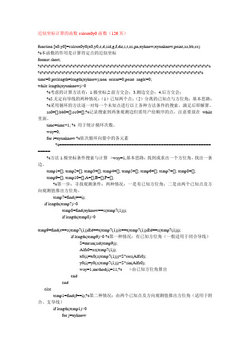
近似坐标计算的函数-calcux0y0函数（126页）function [x0,y0]=calcux0y0(x0,y0,e,d,sid,g,f,dir,s,t,az,pn,xyknow,xyunknow,point,aa,bb,cc)%本函数的作用是计算待定点的近似坐标format short; %%%%%%%%%%%%%%%%%%%%%%%%%%%%%%%%%%%%%%%%%%%%%%% %%%%%%%%%%%%%%%%%%%%%%%%%%%%%%%%%%%%%%%%%%%%% time=0;prelength=length(xyknow);non_orient=0;point_angle=0;while length(xyunknow)>0%考虑的计算方法有：1.极坐标;2.前方交会；3.测边交会；4.后方交会；%5.无定向导线的两种情况：（1）已知两个点；（2）分离的已知点与方位角；基本思路：%采用循环的方法逐一对每一个未知点进行以上各种方法条件的搜索，满足后即解算。

aa0=[];bb0=[];cc0=[];%记录搜索到两条观测边但需用户给顺序的点，注意要放在while 里面。

time=time+1; % 用于统计循环次数。

way=0;for i=xyunknow %依次循环向量中的各元素%============================================================= =====%方法1.极坐标条件搜索与计算-->way=1,基本思路：找到或求出一个方位角，找出一条边。

temp1=[]; temp2=[]; temp3=[]; temp4=[]; temp5=[]; temp6=[]; temp7=[]; temp8=[];temp9=[]; temp10=[];A=[];B=[];P=[];%第一步：寻找观测条件：两种情况：一是有已知方位角；二是由两个已知点及方向观测值推出方位角。

基于MATLAB的控制网平差程序设计--第四章源代码

chkdat函数（72页）function [n1,k]=chkdat(sd,pn,n1)n=length(n1);k=0;for i=1:ni1=0;for j=1:sdif(n1(i)==pn(j))i1=1;n1(i)=j;break;endendif(i1==0)% fprintf(fit2,'%5d %5d\n',i,n1(i)k=1;endendreturnreadlevelnetdata函数（73页）function [ed,dd,sd,gd,pn,h0,k1,k2,h1,s]=readlevelnetdata global filename filepath;global ed dd sd pn gd h0 k1 k2 h1 s k11 k12;k1=[];k2=[];h=[];s=[];[filename,filepath]=uigetfile('*.txt','选择高程数据文件');fid1=fopen(strcat(filepath,filename),'rt');if(fid1==-1)msgbox('Input File or Path is not correct','Warning','warn');return;ended=fscanf(fid1,'%f',1);dd=fscanf(fid1,'%f',1);sd=ed+dd;gd=fscanf(fid1,'%f',1);pn=fscanf(fid1,'%f',sd);h0=fscanf(fid1,'%f',ed);h0(dd+1:ed+dd)=h0(1:ed);heightdiff=fscanf(fid1,'%f',[4,gd]);heightdiff=heightdiff';k1=heightdiff(:,1);%起点k2=heightdiff(:,2);%终点k11=heightdiff(:,1);%起点k12=heightdiff(:,2);%终点h1=heightdiff(:,3);%高差s=heightdiff(:,4);%距离fclose('all');%点号转换[k1,k01]=chkdat(sd,pn,k1);[k2,k02]=chkdat(sd,pn,k2);h0(1:dd)=20000;ie=0;while(1)%计算近似高程for k=1:gdi=k1(k);j=k2(k);if(h0(i)<1e4&h0(j)>1e4)h0(j)=h0(i)+h1(k);ie=ie+1;endif(h0(i)>1e4&h0(j)<1e4)h0(i)=h0(j)-h1(k);ie=ie+1;endendif(ie==dd)break;endendh0=reshape(h0,length(h0),1); returnbm1函数（75页）function id=bm1(gd,dd,k1,k2)%计算一维压缩存放的数组idid=[];for i=1:ddk=i;for j=1:gdi1=k1(j);i2=k2(j);if(i1==i&i2<k)k=i2;endif(i2==i&i1<k)k=i1;endendid(i)=k;endfor i=2:ddid(i)=id(i-1)+i-id(i)+1;endreturn一维压缩存储法方程平差（76页）global pathname filenameglobal ed dd sd pn gd h0 k1 k2 h1 s dh;p=1./s;id=bm1(gd,dd,k1,k2);mm=id(dd);a(1:mm)=0;b(1:dd)=0;for k=1:gd %形成法方程i=k1(k);j=k2(k);h1=h1(k)+h0(i)-h0(j);if(i<=dd)ii=id(i)-i;a(ii+i)=a(ii+i)+p(k);b(i)=b(i)-h1*p(k);endif(j<=dd)jj=id(j)-j;a(jj+j)=a(jj+j)+p(k);b(j)=b(j)+h1*p(k);if(i<=dd)if(i>=j)a(ii+j)=a(ii+j)-p(k);elsea(jj+i)=a(jj+i)-p(k);endendendenda=gs5(dd,a,id);%变带宽下三角紧缩存储高斯消元法dh=cy6(a,b,id,dd,1);%常数项约化与回代子程序dh(dd+1:ed+dd)=0;hm(dd+1:ed+dd)=0;for i=1:sdh(i)=h0(i)+dh(i);endvv=0;for i=1:gdL(i)=h(k2(i))-h(k1(i));v(i)=h(k2(i))-h(k1(i))-h1(i);vv=vv+v(i)*v(i)/s(i);endu=sqrt(vv/(gd-dd));for i=1:ddb(1:dd)=0;b(i)=1.0;b=cy6(a,b,id,dd,i);hm(i)=sqrt(b(i))*u;endwritelevelnetdata(pn,k1,k2,h1,v',L',h0,dh',h',hm',u);gs5函数（77页）function a=gs5(dd,a,id)%变带宽高斯消去法for i=1:ddii=id(i)-i;if(i-1==0)li=1-ii;elseli=id(ii-1)-ii+1;endfor j=li:ijj=id(j)-j;if(j-1)==0lj=1-jj;elselj=id(j-1)-jj+1;endlk=li;if(li<lj)lk=lj;endfor k=lk:j-1kk=id(k);a(ii+j)=a(ii+j)-a(ii+k)/a(kk)*a(jj+k);endendendreturncy6函数（78页）function b=cy6(a,b,id,dd,k1)%常数项约化与回代子程序for i=k1:ddii=id(i)-i;if(i==1)nd=id(i);elsend=id(i)-id(i-1);ende=0;for k=1:i-1if((i-k)<nd)e=e+a(ii+k)*b(k);endendb(i)=(b(i)-e)/(a(ii+i);endfor i=dd-1:-1:k1ii=id(i);for k=i+1:ddkk=id(k)-k;nk=id(k)-id(k-1);if(k-i<nk)b(i)=b(i)-a(kk+i)/a(ii)*b(k);endendendreturn上三角存储法方程平差程序（79页）mm=(dd+1)*dd/2;a(1:mm)=0;b(1:dd)=0;for k=1:gdi=k1(k);j=k2(k);h1=h1(k)+h0(i)-h0(j);if(i<=dd)ii=(i-1)*(dd-i/2);a(ii+i)=a(ii+i)+1/s(k);b(i)=b(i)+1./s(k)*h1;endif(j<=dd)jj=(j-1)*(dd-j/2);a(jj+j)=a(jj+j)+1/s(k);b(j)=b(j)-1./s(k)*h1;if(i<=dd)if(i<j)a(ii+j)=a(ii+j)-1/s(k);elsea(jj+i)=a(jj+i)-1/s(k);endendendenda=invsqr(a,dd);for i=1:dddh(i)=0;di=(i-1)*(dd-i/2);for j=1:dddj=(j-1)*(dd-j/2);if(j<i)dh(i)=dh(i)-a(dj+i)*b(j);elsedh(i)=dh(i)-a(di+j)*b(i);endendenddh(dd+1:ed+dd)=0;hm(dd+1:ed+dd)=0;for i=1:sdh(i)=h0(i)+dh(i);endvv=0;for i=1:gdL(i)=h(k2(i))-h(k1(i));v(i)=h(k2(i))-h(k1(i))-h1(i);vv=vv+v(i)*v(i)/s(i);enduw0=sqrt(vv/(gd-dd));for i=1:ddii=(i-1)*(dd-i/2);hm(i)=sqrt(a(ii+i))*uw0;endreturn输出数据函数（79页）function writelevelnetdata(pn,k1,k2,h1,v,L,h0,dh,h,hm,uw0)disp('待定点高程平差值及中误差:')disp('---点号----近似高程(m)-高程改正(m)-高程平差值(m)-中误差')[pn,h0,dh,h,hm]disp('高差观测值平差值:')disp('---点号------点号----观测高差(m)---高差改正(m)-平差高差(m)')[pn(k1),pn(k2),h1,v,L][filename1,pathname1]=uigetfile('*.txt','请选择输出文件');fid2=fopen(strcat(pathname1,filename1),'wt');if(fid2==-1)msgbox('Error by Opening Output File','Warning','warn');return;endfprintf(fid2,'待定点高程平差值及中误差：\n 点号--近似高程(m)--高程改正(m)-高程平差值(m)-中误差\n');fprintf(fid2,'%5d %10.4f %10.4f %10.4f %10.4f\n',[pn,h0,dh,h,hm]');fprintf(fid2,'高差观测值平差值:\n -点号---点号--观测高差(m)--高差改正(m)-平差高差(m)\n'); fprintf(fid2,'%5d %5d %10.4f %10.4f %10.4f\n',[pn(k1),pn(k2),h1,v,L]');fprintf(fid2,'单位权中误差：%10.4fm\n',uw0);% open(strcat(pathname1,filename1));fclose(fid2);return利用Matlab矩阵运算的平差程序（81页）function level3ticdisp('平差已经开始---->>>>')global ed dd sd pn gd h0 k1 k2 h1 s dh;[ed,dd,sd,gd,pn,h0,k1,k2,h1,s]=readlevelnetdata;[dh,h,V,L,uw0,uwh,uwl]=calculatelevelnet(ed,dd,sd,gd,pn,h0,k1,k2,h1,s);writelevelnetdata(pn,k1,k2,h1,V,L,h0,dh,h,uwh,uw0); %输出水准网解算结果yunxing=toc;disp(['平差过程的运行时间为',num2str(yunxing),'秒。

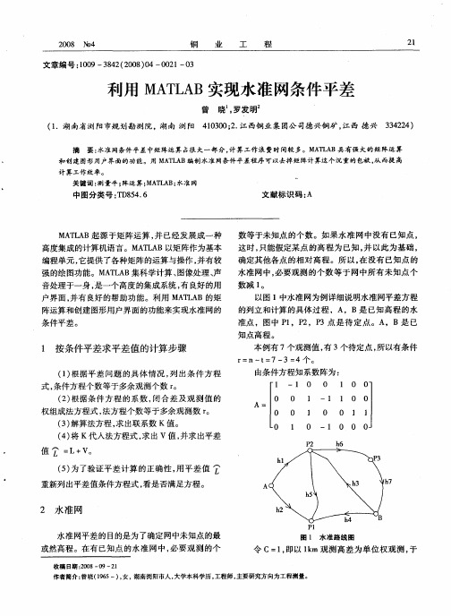
利用MATLAB实现水准网条件平差

０
Ｐ２ｈ６
（）Ｋ代入法方程式，出Ｖ值，４将求并求出平差值＝ＶＬ＋。（）５为了验证平差计算的正确性，用平差值重新列出平差值条件方程式，看是否满足方程。
Ａ
ｈ７
２水准网
Ｐ１
铜
业
工
程
２０Ｎ４０８０
是＝，＝Ｑ
＝５。因各观测高差不相关故
协因数阵为对角阵，：即
１７．２．３
Ｑ＝Ｐ＝～
２．７
２４．
１４．
１６．
由此组成法方程为：
ｒ．５２２４．２４．０１７．
强的绘图功能。ＭＴＡＡＬＢ集科学计算、图像处理、声
音处理于一身，一个高度的集成系统，良好的用是有户界面，并有良好的帮助功能。利用ＭＡＬＢ的矩ＴＡ
水准网中，必要观测的个数等于网中所有未知点个
数减ｌ。以图１中水准网为例详细说明水准网平差方程的列立和计算的具体过程，Ａ，Ｂ是已知高程的水准点，图中Ｐ，Ｐ，Ｐｌ２３点是待定点。Ａ，Ｂ是已
摘
要：水准网条件平差中矩阵运算占很大一部分，计算工作浪费时间较多。ＭＡＬＢ具有强大的矩阵运算ＴＡ
和创建图形厨户界面的功能。用ＭＡＬＢ编制水准网条件平差程序可以去掉矩阵计算这个沉重的包袱，而提高ＴＡ从
计算工作效率。
关键词：测量平；阵运算；ＴＡ；ＭＡＬＢ水准网

基于MATLAB的控制网平差程序设计--第五章源代码 - 副本

观测数据读入程序，rddat1函数（85页）global net ed dd sd dd1 pn x0 y0 m1 m2 m3 ms pp e d sid md g f dir ni si ma s t az aa bb cc rt rr tt global pathname filenamex0=[];y0=[];e=[];d=[];sid=[];g=[];f=[];dir=[];si=[];ni=[];s=[];t=[];az=[];pn=[];[filename,pathname]=uigetfile('*.txt','请选择原始数据');fit1=fopen(strcat(pathname,filename),'rt');if(fit1==-1)msgbox('Input File or Path is not correct','Warning','warn');return;endnet=fscanf(fit1,'%d',1);[a]=fscanf(fit1,'%d',3);ed=a(1);dd=a(2);dd1=a(3);sd=ed+dd;[pn]=fscanf(fit1,'%d',sd);[a]=fscanf(fit1,'%f',2*ed);for i=1:edx0(i)=a(2*i-1);y0(i)=a(2*i);end[a]=fscanf(fit1,'%d',3);m1=a(1);m2=a(2);m3=a(3);isid=0;[a]=fscanf(fit1,'%f',2);ms=a(1);pp=a(2);[a]=fscanf(fit1,'%d %d %f',3*m1);for i=1:m1e(i)=a(3*i-2);d(i)=a(3*i-1);sid(i)=a(3*i);end[e,i1]=chkdat(sd,pn,e);[d,i2]=chkdat(sd,pn,d);i3=0;isid=i1+i2+i3;idir=0;md=fscanf(fit1,'%f',1);[a]=fscanf(fit1,'%d %d %f',3*m2);for i=1:m2n1(i)=a(3*i-2);n2(i)=a(3*i-1);unk(i)=a(3*i);end[n1,i1]=chkdat(sd,pn,n1);[n2,i2]=chkdat(sd,pn,n2);i3=0;ik=1;si(1)=1;for i=1:sdii=0;for j=1:m2if(n1(j)==j)ii=ii+1;g(ik)=n1(j);f(ik)=n2(j);dir(ik)=unk(j);ik=ik+1;endendni(i)=ii;si(i+1)=si(i)+ni(i);endidir=i1+i2+i3;iaz=0;if(m3>0)ma=fscanf(fit1,'%f',1);[a]=fscanf(fit1,'%d %d %f',3*m3);for i=1:m3s(i)=a(3*i-2);t(i)=a(3*i-1);az(i)=a(3*i);end[s,i1]=chkdat(sd,pn,s);[t,i2]=chkdat(sd,pn,t);i3=0;iaz=i1+i2+i3;endkk=isid+idir+iaz;if(kk>0)msgbox('Error by function rddat1','Warning','warn');return;endfclose('all');open(strcat(pathname,net_name,b_datafile));return误差方程与法方程的组成函数-obnorm函数（90页）function obnormglobal ed dd dd1 ni si e d g f s tglobal m1 m2 m3 ms pp md ma x0 y0 sid dir az c fit1 fit2 global a q1 pa3 qls wlo=2062.648062470964;m=m1+m2+m3;n=2*dd;sum=n*(n+1)/2.0;sd=ed+dd;a(1:m,1:9)=0.0;for i=1:sdii=4*(ni(i)+1);pa3(i,1:ii)=0.0;endc(1:sum)=0.0;w(1:n)=0.0;for i=1:m1 %边长观测误差方程dx=x0(d(i))-x0(e(i));dy=y0(d(i))-y0(e(i));ss=sqrt(dx*dx+dy*dy);cosa=dx/ss;sina=dy/ss;a(i,1)=2*e(i)-1-2*ed+1.0e-9;a(i,2)=-cosa;a(i,3)=a(i,1)+1;a(i,4)=-sina;a(i,5)=2*d(i)-1-2*ed+1.0e-9;a(i,6)=cosa;a(i,7)=a(i,5)+1;a(i,8)=sina;a(i,9)=100.0*(ss-sid(i));q1(i)=(ms^2+(ss*pp*0.0001)^2);endq1(m1+1:m2+m1)=md*md;for i=1:sdif(ni(i)==0)continue;endjj=5;z0=0.0;zal=0;for j=si(i):s(i)+ni(i)-1dx=x0(f(j))-x0(g(j));dy=y0(f(j))-y0(g(j));a0=alfa(dx,dy);z1=a0-dir(j);if(z1<=0.0)z1=z1+2.0*pi;endzal=zal+1./ql(m1+j);z0=z0+z1/q1(m1+j);endz0=z0/zal;for j=si(i):si(i)+ni(i)-1dx=x0(f(j))-x0(g(j));dy=y0(f(j))-y0(g(j));ss=dx*dx+dy*dy;a0=alfa(dx,dy);ai=-dy/ss*lo;bi=dx/ss*lo;ii=m1+j;a(ii,1)=2*g(j)-1-2*ed+1.0e-9;a(ii,2)=-ai;a(ii,3)=a(ii,1)+1;a(ii,4)=-bi;a(ii,5)=2*f(j)-1-2*ed+1.0e-9;a(ii,6)=ai;a(ii,7)=a(ii,5)+1;a(ii,8)=bi;ss=dir(j)+z0;if(ss>=2.0*pi)ss=ss-2.0*pi;enda(ii,9)=(a0-ss)*lo*100.0;pa3(i,jj)=a(ii,5);pa3(i,jj+1)=a(ii,6)/q1(ii);pa3(i,jj+2)=a(ii,7);pa3(i,jj+3)=a(ii,8)/q1(ii);pa3(i,2)=pa3(i,2)+a(ii,2)/q1(ii);pa3(i,4)=pa3(i,4)+a(ii,4)/q1(ii);jj=jj+4;endpa3(i,1)=a(ii,1);pa3(i,3)=a(ii,3);qls(i)=-zal;endfor i=1:m3dx=x0(t(i))-x0(s(i));dy=y0(t(i))-y0(s(i));a0=alfa(dx,dy,a0);ss=dx*dx+dy*dy;ai=-dy/ss*lo;bi=dx/ss*lo;ii=m1+m2+i;a(ii,1)=2*s(i)-1-2*ed+1.0e-9;a(ii,2)=-ai;a(ii,3)=a(ii,1)+1;a(ii,4)=-bi;a(ii,5)=2*t(i)-1-2*ed+1.0e-9;a(ii,6)=ai;a(ii,7)=a(ii,5)+1;a(ii,8)=bi;if((a0-az(i))>pi)a(ii,9)=(a0-az(i)-2.0*p)*lo*100;elsea(ii,9)=(a0-az(i))*lo*100.0;endq1(ii)=ma*ma;endfor i=1:m %形成法方程for j=1:4jj=fix(a(i,2*j-1));if(jj<=0)continue;endw(jj)=w(jj)+a(i,2*j)*a(i,9)/q1(i);di=(jj-1)*(n-jj/2.0);for k=1:4kk=fix(a(i,2*k-1));if(kk<=0|jj>kk)continue;endc(di+kk)=c(di+kk)+a(i,2*k)*a(i,2*j)/q1(i);endendendif(m2>0) %和误差方程形成法方程for i=1:sdif(ni(i)==0)continue;endfor j=1:2*(ni(i)+1)jj=fix(pa3(i,2*j-1));if(jj<=0)continue;enddi=(jj-1)*(n-jj/2);for k=1:2*(ni(i)+1)kk=fix(pa3(i,2*k-1));if(kk<=0|jj>kk)continue;endc(di+kk)=c(di+kk)+pa3(i,2*k)*pa3(i,2*j)/qls(i);endendendendreturn平差值与精度评定（94页）global net ed dd sd dd1 pn x0 y0 m1 m2 m3 ms pp e d sid md g f dir ni si ma s t az global aa bb cc rt rr ttglobal a q1 pa3 qls w c x y uw0global pathname net_name s_datafile a_datafile;fit2=fopen(strcat(pathname,net_name,a_datafile,'wt');if(fit2==-1)msgbox('Input File or Path is not correct','Warning','warn');return;endk=1;while(k)m=m1+m2+m3;obnorm;c=invsqr(c,2*dd);[uw0,k]=adjxy(fit2);endellipse(uw0,fit2);n=2*dd;sum=n*(n+1)/2.0;n1=2*(ed+dd);sum1=n1*(n1+1)/2.0;for i=sum1:-1:sum1-sum+1c(i)=c(i-(sum1-sum));endfor i=1:2*eddi=(i-1)*(n1-i/2.0);for j=i:n1if(j==i)c(di+j)=0.00000001;elsec(di+j)=0.0;endendendif(m1>0)adjs(uw0,fit2);endif(m2>0)adjd(uw0,fit2);endif(m3>0)adja(uw0,fit2);endfclose(fit2);open(strcat(pathname,net_name,a_datafile));坐标改正数计算及单位权中误差计算函数-adjxy函数（95页）function [uw0,k]=adjxy(fit2)global ed dd dd1 ni si e d g f s t pn x yglobal m1 m2 m3 ms md ma x0 y0 sid dir az cglobal a q1 pa3 qls wsd=ed+dd;n=2*dd;k=0;for i=1:ndxy(i)=0.0;di=(i-1)*(n-i/2.0);for j=1:ndj=(j-1)*(n-j/2.0);if(j<i)dxy(i)=dxy(i)-c(dj+i)*w(j);elsedxy(i)=dxy(i)-c(di+j)*w(j);endendif(abs(dxy(i))>1.0)k=1;enddxy(i)=dxy(i)/100.0;endx(1:ed)=x0(1:ed);y(1:ed)=y0(1:ed);for i=1:ddx(ed+i)=x0(ed+i)+dxy(2*i-1);y(ed+i)=y0(ed+i)+dxy(2*i);endx0(1:sd)=x(1:sd);y0(1:sd)=y(1:sd);for i=1:sdif(i<=ed)vx(i)=0.0;vy(i)=0.0;elsevx(i)=dxy(2*(i-ed)-1);vy(i)=dxy(2*(i-ed));endendfprintf(fit2,' adjusted coordinates\n');fprintf(fit2,' pn vx x vy y\n');for i=1:sdfprintf(fit2,' %6d %8.4f %14.4f %8.4f %14.4f\n',pn(i),vx(i),x(i),vy(i),y(i));endpvv=0.0;for i=1:npvv=pvv+w(i)*dxy(i)*100.0;endm=m1+m2+m3;for i=1:mpvv=pvv+a(i,9)*a(i,9)/ql(i);endif(m2>0)ii=0;for i=1:sdif(ni(i)~=0;ii=ii+1;endendenduw0=sqrt(pvv/((m-n-ii)*1.0e0));return计算各点误差椭圆-ellipse函数（98页）function ellipse(uw0,fit2)glosbal ed dd pn c x y ai bi fifprintf(fit2,' parameter of error ellipse\n');fprintf(fit2,' pn(i) mx my mm a b fi\n'); n=2.0*dd;maxmm=0.0;smm=0.0;for i=1:ddii=ed+i;di=(2*i-2)*(n-(2*i-1)/2.0);dj=(2*i-1)*(n-i);q1=c(di+2*i-1);q2=c(dj+2*i);q3=c(di+2*i);d1=sqrt(abs(q1+q2-q3));d=uw0*dl;xx=q1-q2;yy=2*q3;zz=q1+q2;mx1=sqrt(q1);my1=sqrt(q2);mm1=sqrt(zz);if(abs(xx)<1d-10)fi(i)=sign(90.0,q3);elsefi(i)=atan(yy/xx)*57.2958;endif(xx>=0&yy>=0)fi(i)=fi(i)/2.0;elseif(xx>=0&yy<=0)fi(i)=(fi(i)+360)/2.0;elseif(xx<0)fi(i)=(fi(i)+180)/2.0;endww=sqrt(xx*xx+yy*yy);a1=sqrt((zz+ww)/2.0);b1=sqrt((zz-ww)/2.0);ab1=a1-b1;mx=uw0*mx1;my=uw0*my1;mm=uw0*mm1;if(mm>maxmm)maxmm=mm;i1=ii;endsmm=smm+mm;ai(i)=uw0*a1;bi(i)=uw0*b1;ab=ai(i)-bi(i);fprintf(fit2,' %10d %10.3f %10.3f %10.3f %10.3f %10.3f %10.3f\n',pn(ii),mx,my,mm,ai(i),bi(i),fi(i));endsmm=smm/dd;fprintf(fit2,' mse of unit weight= %9.6f\n',uw0);fprintf(fit2,' the maximum station error mm= %8.3f(cm) pn= %4d\n',maxmm,pn(i1));fprintf(fit2,' the average station error mm= %8.3f\n',smm);return边长观测值平差值改正数及精度评定-adjs函数（101页）function adjs(uw,fit2)global ed dd sd pn m1 e d sid x yfprintf(fit2,'adjusted sides\n');fprintf(fit2,'i pn(e) pn(d) side vs(cm) side+vs ms\n');for i=1:m1dx=x(d(i))-x(e(i));dy=y(d(i))-y(e(i));if(e(i)<d(i))[maa,mss]=trel(uw,e(i),d(i));else[maa,mss]=trel(uw,d(i),e(i));endss=dx*dx+dy*dy;ss=sqrt(ss);vs=(ss-sid(i))*100;sid1=sid(i)+vs/100;fprintf(fit2,' %3d %8d %8d %15.4f %10.4f %15.4f %8.2f\n',i,pn(e(i)),pn(d(i)),sid(i),vs,sid1,mss);endreturn方向观测值的平差与精度评定-adjd函数（102页）function adjd(uw,fit2)global ed dd dd1 sd pn ni si e d g f s t netglobal m1 m2 m3 ms pp md ma x0 y0 x y sid dir az cglobal a q1 pa3 qls wfprintf(fit2,'adusted directions and their accuracy\n');fprintf(fit2,' i pn(g) pn(f) dir vd(") dir+vd\n');lo=206264.8062470964;for j=1:m2q1(j+m1)=md*md;endfor i=1:sdzi=0.0;zal=0.0;for j=si(i):si(i)+ni(i)-1dx=x(f(j))-x(g(j));dy=y(f(j))-y(g(j));a0=alfa(dx,dy);z1=a0-dir(j);if(z1<0.0)z1=z1+2.0*pi;endzal=zal+1./ql(m1+j);zi=zi+z1/ql(m1+j);endif(ni(i)~=0)zi=zi/zal;endfor j=si(i):si(i)+ni(i)-1dx=x(f(j))-x(g(j));dy=y(f(j))-y(g(j));a0=alfa(dx,dy);ss=dir(j)+zi;if(ss>=2.0*pi)ss=ss-2*pi;endvd=(a0-ss)*lo;dir1=dir(j)+vd/lo;dir1=rad_dms(dir1);dir(j)=rad_dms(dir(j));fprintf(fit2,' %3d %8d %8d %14.5f %9.2f %16.5f\n', j,pn(g(j)),pn(f(j)),dir(j),vd,dir1);endendfprintf(fit2,'adusted directions\n');fprintf(fit2,' i pn(g) pn(f) dir az ma\n');for i=1:sdfor j=si(i):si(i)+ni(i)-1dx=x(f(j))-x(g(j));dy=y(f(j))-y(g(j));if(f(j)<g(j))[maa,mss]=trel(uw,f(j),g(j));else[maa,mss]=trel(uw,g(j),f(j));enda0=alfa(dx,dy);if(j==si(i))a00=a0;endss=a0-a00;if(ss<0)ss=ss+2.0*pi;endss=rad_dms(ss);a0=rad_dms(a0);fprintf(fit2,' %3d %10d %10d %14.5d %14.5d %10.4f\n',j,pn(g(j)),pn(f(j)),ss,a0,maa);endendreturn方位角观测值改正数与精度评定-adja函数（104页）function adja(uw,fit2)global m3 x y s t azl0=206264.8062470964;fprintf(fit2,'adjusted azimath \n i pn(s) pn(t) az va(") az+va ma');for i=1:m3dx=x(t(i))-x(s(i));dy=y(t(i))-y(s(i));a0=alfa(dx,dy);if(t(i)<s(i))[maa,mss]=trel(uw,t(i),s(i));else[maa,mss]=trel(uw,s(i),t(i));endif((a0-az(i))>pi)va=(a0-az(i)-2*pi)*lo;elseva=(a0-az(i))*lo;endaz1=az(i)+va/lo;az1=wg(az1);az(i)=wg(az(i));fprintf(fit2,' %3d %8d %8d %13.5f %8.2f %12.5f %8.2f',i,pn(s(i)),pn(t(i)),az(i),va,az1,maa);endreturn调用的的trel函数function [maa,mss]=trel(uw,rr,tt)global ed dd x0 y0 pn cn=2*(dd+ed);dx=x0(tt)-x0(rr);dy=y0(tt)-y0(rr);ss=sqrt(dx*dx+dy*dy);a0=alfa(dx,dy);aij=2062.648*sin(a0)/ss;bij=-2062.648*cos(a0)/ss;b=a+1;f=2*tt-1;g=f+1;da=(a-1)*(n-a/2.0);db=(b-1)*(n-b/2.0);df=(f-1)*(n-f/2.0);dg=(g-1)*(n-g/2.0);q1=c(da+a)+c(df+f)-2.0*c(da+f);q2=c(db+b)+c(dg+g)-2.0*c(db+g);q3=c(da+b)+c(df+g)-c(da+g)-c(db+f);x=q1-q2;y=2.0*q3;z=q1+q2;qs=q1*cos(a0)^2+q2*sin(a0)^2+q3*sin(2.0*a0); qa=q1*aij*aij+q2*bij*bij+2.0*q3*aij*bij;ms=sqrt(qs)*uw;maa=sqrt(qa)*uw;return。

matlab常见经典平差程序

matlab常见经典平差程序希望本人编写的经典平差可以对matlab初学者以及测绘专业的学生有用By cowboyfunction void()sprintf('请选择平差类型')sprintf('1: 参数平差\n2: 条件平差\n3：具有条件的参数平差\n4: 具有参数的条件平差\n') a=input('请输入对应号码\n');switch (a)case 1% 参数平差V=AX-Lsprintf('1:参数平差V=AX-L')n=input('请输入n=');t=input('请输入t=');A=input('请输入系数矩阵A=');L=input('请输入常数项矩阵L=');P=diag(input('请输入权阵P='))%P=input('请输入权阵P=');N=A'*P*A;U=A'*P*L;sprintf('开始计算')X=inv(N)*(U);V=A*X-L;Qx=inv(N);u=sqrt((V'*P*V)/(n-t));fid=fopen('data.txt','wt'); %写入文件路径，文件输出fprintf(fid,'=====================参数平差: V=AX-L =====================\n');fprintf(fid,'输出n,t\n') ;fprintf(fid,'%12.5f %12.5f\n',n ,t) ;%n,t fprintf(fid,'输出矩阵A\n')[m,n]=size(A); %Afor i=1:1:mfor j=1:1:nif j==nfprintf(fid,'%12.5f\n',A(i,j));elsefprintf(fid,'%12.5f\t',A(i,j));endendendfprintf(fid,'\n');fprintf(fid,'输出矩阵L\n') ;[m,n]=size(L); %Lfor i=1:1:mfor j=1:1:nif j==nfprintf(fid,'%12.5f\n',L(i,j));elsefprintf(fid,'%12.5f\t',L(i,j));endendendfprintf(fid,'\n');fprintf(fid,'输出矩阵P\n') ;[m,n]=size(P); %P for i=1:1:mfor j=1:1:nif j==nfprintf(fid,'%12.5f\n',P(i,j));elsefprintf(fid,'%12.5f\t',P(i,j));endendendfprintf(fid,'\n');fprintf(fid,'输出矩阵X\n'); [m,n]=size(X); %X for i=1:1:m for j=1:1:nif j==nfprintf(fid,'%12.5f\n',X(i,j));elsefprintf(fid,'%12.5f\t',X(i,j));endendendfprintf(fid,'\n');fprintf(fid,'输出矩阵V\n'); [m,n]=size(V); %V for i=1:1:m for j=1:1:nif j==nfprintf(fid,'%12.5f\n',V(i,j));elsefprintf(fid,'%12.5f\t',V(i,j));endendendfprintf(fid,'\n');fprintf(fid,'输出矩阵Qx\n'); [m,n]=size(Qx); %Qx for i=1:1:mfor j=1:1:nif j==nfprintf(fid,'%12.5f\n',Qx(i,j)); elsefprintf(fid,'%12.5f\t',Qx(i,j));endendendfprintf(fid,'\n');fprintf(fid,'输出单位权中误差u\n'); [m,n]=size(u); %u for i=1:1:m for j=1:1:nif j==nfprintf(fid,'%12.5f\n',u(i,j));elsefprintf(fid,'%12.5f\t',u(i,j));endendendfprintf(fid,'\n');fclose(fid);case 2% 条件平差BV+W=0sprintf('2:条件平差BV+W=0')n=input('请输入n=');t=input('请输入t=');B=input('请输入系数矩阵B=');W=input('请输入自由项向量W='); P=input('请输入权阵P='); sprintf('开始计算')K=-inv((B*inv(P)*B'))*W;V=inv(P)*B'*K;u=sqrt((V'*P*V)/(n-t));Ql=inv(P)-inv(P)*B'*inv(B*inv(P)*B')*B*inv(P);fid=fopen('data.txt','wt'); %写入文件路径，文件输出fprintf(fid,'=====================条件平差: BV+W=0 =====================\n'); fprintf(fid,'输出n,t\n') ;fprintf(fid,'%12.5f %12.5f\n',n ,t) ;%n,tfprintf(fid,'输出矩阵B\n');[m,n]=size(B); %Bfor i=1:1:mfor j=1:1:nif j==nfprintf(fid,'%12.5f\n',B(i,j));elsefprintf(fid,'%12.5f\t',B(i,j));endendendfprintf(fid,'\n');fprintf(fid,'输出矩阵W\n');[m,n]=size(W); %Wfor i=1:1:mfor j=1:1:nif j==nfprintf(fid,'%12.5f\n',W(i,j));elsefprintf(fid,'%12.5f\t',W(i,j));endendendfprintf(fid,'\n');fprintf(fid,'输出矩阵P\n'); [m,n]=size(P); %Pfor i=1:1:mfor j=1:1:nif j==nfprintf(fid,'%12.5f\n',P(i,j)); elsefprintf(fid,'%12.5f\t',P(i,j));endendendfprintf(fid,'\n');fprintf(fid,'输出矩阵V\n'); [m,n]=size(V); %Vfor i=1:1:mfor j=1:1:nif j==nfprintf(fid,'%12.5f\n',V(i,j)); elsefprintf(fid,'%12.5f\t',V(i,j)); endendendfprintf(fid,'\n');fprintf(fid,'输出矩阵Qx\n'); [m,n]=size(Ql); %Ql for i=1:1:m for j=1:1:nif j==nfprintf(fid,'%12.5f\n',Ql(i,j));elsefprintf(fid,'%12.5f\t',Ql(i,j));endendendfprintf(fid,'\n');fprintf(fid,'输出单位权中误差u\n');[m,n]=size(u); %u for i=1:1:mfor j=1:1:nif j==nfprintf(fid,'%12.5f\n',u(i,j));elsefprintf(fid,'%12.5f\t',u(i,j));endendendfprintf(fid,'\n');fclose(fid);case 3% 具有条件的参数平差% 参数平差V=AX-L% 条件平差BX+W=0sprintf('3:具有条件的参数平差V=AX-L;BX+W=0') n=input('请输入n=');t=input('请输入t=');r=input('请输入r=');A=input('请输入误差方程系数矩阵A=');L=input('请输入常数项矩阵L=');B=input('请输入条件方程系数矩阵B=');W=input('请输入自由项向量W=');P=input('请输入权阵P=');sprintf('开始计算')K=-(inv(B*inv(A'*P*A)*B'))*(W+B*inv(A'*P*A)*A'*P*L)X=(inv(A'*P*A))*(B'*K+A'*P*L)N=(A'*P*A)M=B*inv(N)*B'Qx=inv(N)-inv(N)*B'*inv(M)*B*inv(N)u=sqrt((V'*P*V)/(n-t+r))fid=fopen('data.txt','wt'); %写入文件路径，文件输出fprintf(fid,'=====================具有条件的参数平差: V=AX-L;BX+W=0 ===========================\n');fprintf(fid,'输出n,t,r\n') ;fprintf(fid,'%12.5f %12.5f %12.5f\n',n ,t,r); %n,t,rfprintf(fid,'输出矩阵A\n');[m,n]=size(A); %Afor i=1:1:mfor j=1:1:nif j==nfprintf(fid,'%12.5f\n',A(i,j));elsefprintf(fid,'%12.5f\t',A(i,j));endendendfprintf(fid,'\n');fprintf(fid,'输出矩阵L\n');[m,n]=size(L); %Lfor i=1:1:mfor j=1:1:nif j==nfprintf(fid,'%12.5f\n',L(i,j)); elsefprintf(fid,'%12.5f\t',L(i,j)); endendendfprintf(fid,'\n');fprintf(fid,'输出矩阵B\n'); [m,n]=size(B); %Bfor i=1:1:mfor j=1:1:nif j==nfprintf(fid,'%12.5f\n',B(i,j)); fprintf(fid,'%12.5f\t',B(i,j)); endendendfprintf(fid,'\n');fprintf(fid,'输出矩阵W\n'); [m,n]=size(W); %W for i=1:1:m for j=1:1:nif j==nfprintf(fid,'%12.5f\n',W(i,j)); elsefprintf(fid,'%12.5f\t',W(i,j)); endendendfprintf(fid,'\n');fprintf(fid,'输出矩阵P\n'); [m,n]=size(P); %P for i=1:1:m for j=1:1:nif j==nfprintf(fid,'%12.5f\n',P(i,j)); elsefprintf(fid,'%12.5f\t',P(i,j)); endendendfprintf(fid,'\n');fprintf(fid,'输出矩阵X\n'); [m,n]=size(X); %X for i=1:1:m for j=1:1:nif j==nfprintf(fid,'%12.5f\n',X(i,j)); elsefprintf(fid,'%12.5f\t',X(i,j)); endendendfprintf(fid,'\n');fprintf(fid,'输出矩阵V\n'); [m,n]=size(V); %Vfor j=1:1:nif j==nfprintf(fid,'%12.5f\n',V(i,j)); elsefprintf(fid,'%12.5f\t',V(i,j));endendendfprintf(fid,'\n');fprintf(fid,'输出矩阵Qx\n'); [m,n]=size(Qx); %Qx for i=1:1:m for j=1:1:nif j==nfprintf(fid,'%12.5f\n',Qx(i,j)); elsefprintf(fid,'%12.5f\t',Qx(i,j)); endendendfprintf(fid,'\n');fprintf(fid,'输出单位权中误差\n'); [m,n]=size(u); %u for i=1:1:m for j=1:1:nif j==nfprintf(fid,'%12.5f\n',u(i,j));elsefprintf(fid,'%12.5f\t',u(i,j));endendendfprintf(fid,'\n');fclose(fid);case 4% 具有参数的条件平差% 具有参数的条件方程式BV+AX+W=0sprintf('4:具有参数的条件平差BV+AX+W=0 ')n=input('请输入n=');t=input('请输入t=');r=input('请输入r=');B=input('请输入条件方程中V的系数矩阵B=');A=input('请输入条件方程中X的系数矩阵A=');W=input('请输入条件方程自由向量W=');P=input('请输入权阵P=');sprintf('开始计算')N=(B*inv(P)*B')M=(A'*inv(N)*A)X=-inv(M)*A'*inv(N)*WK=-inv(N)*(A*X+W)V=inv(P)*B'*KQx=inv(M)u=sqrt((V'*P*V)/(r-t))fid=fopen('data.txt','wt'); %写入文件路径，文件输出fprintf(fid,'=====================具有参数的条件平差: BV+AX+W=0 ================================\n');fprintf(fid,'输出n,t,r\n') ;fprintf(fid,'%12.5f %12.5f %12.5f\n',n ,t,r) ; %n,t,rfprintf(fid,'输出矩阵B\n');[m,n]=size(B); %Bfor i=1:1:mfor j=1:1:nif j==nfprintf(fid,'%12.5f\n',B(i,j));elsefprintf(fid,'%12.5f\t',B(i,j)); endendendfprintf(fid,'\n');fprintf(fid,'输出矩阵A\n'); [m,n]=size(A); %Afor i=1:1:mfor j=1:1:nif j==nfprintf(fid,'%12.5f\n',A(i,j)); elsefprintf(fid,'%12.5f\t',A(i,j)); endendendfprintf(fid,'\n');fprintf(fid,'输出矩阵W\n'); [m,n]=size(W); %Wfor i=1:1:mfor j=1:1:nif j==nfprintf(fid,'%12.5f\n',W(i,j)); elsefprintf(fid,'%12.5f\t',W(i,j)); endendendfprintf(fid,'\n');fprintf(fid,'输出矩阵P\n');[m,n]=size(P); %P for i=1:1:m for j=1:1:nif j==nfprintf(fid,'%12.5f\n',P(i,j)); elsefprintf(fid,'%12.5f\t',P(i,j)); endendendfprintf(fid,'\n');fprintf(fid,'输出矩阵X\n'); [m,n]=size(X); %X for i=1:1:m for j=1:1:nif j==nfprintf(fid,'%12.5f\n',X(i,j)); elsefprintf(fid,'%12.5f\t',X(i,j)); endendendfprintf(fid,'\n');fprintf(fid,'输出矩阵V\n'); [m,n]=size(V); %V for i=1:1:m for j=1:1:nif j==nfprintf(fid,'%12.5f\n',V(i,j)); elsefprintf(fid,'%12.5f\t',V(i,j)); endendendfprintf(fid,'\n');fprintf(fid,'输出矩阵Qx\n'); [m,n]=size(Qx); %Qx for i=1:1:m for j=1:1:nif j==nfprintf(fid,'%12.5f\n',Qx(i,j)); elsefprintf(fid,'%12.5f\t',Qx(i,j)); endendendfprintf(fid,'\n');fprintf(fid,'输出单位权中误差\n'); [m,n]=size(u); %u for i=1:1:m for j=1:1:nif j==nfprintf(fid,'%12.5f\n',u(i,j));elsefprintf(fid,'%12.5f\t',u(i,j));endendendfprintf(fid,'\n');fclose(fid);otherwisedisp('代号输入有误')end。

实验三-利用matlab程序设计语言完成某工程导线网平差计算

实验三利用mat lab程序设计语言完成某工程导线网平差计算实验数据；某工程项目按城市测量规范(CJJ8-99)不设一个二级导线网作为首级平面控制网，主要技术要求为：平均边长200cm，测角中误差±8,导线全长相对闭合差＜1/10000,最弱点的点位中误差不得大于5cm，经过测量得到观测数据，设角度为等精度观测值、测角中误差为山=±8秒，鞭长光电测距、测距中误差为m二± Vsmm，根据所学的‘误差理论与测量平差基础'提出一个最佳的平差方案，利用matlab完成该网的严密平差级精度评定计算；平差程序设计思路：1采用间接平差方法，12个点的坐标的平差值作为参数.利用matlab进行坐标反算，求出已知坐标方位角；根据已知图形各观测方向方位角；2计算各待定点的近似坐标，然后反算出近似方位角，近似边. 计算各边坐标方位角改正数系数；3确定角和边的权,角度权Pj=1 ；边长权Ps=100/S；4计算角度和边长的误差方程系数和常数项，列出误差方程系数矩阵 B，算出Nbb=B’ PB,W=B’ Pl,参数改正数 x=inv(Nbb)*W;角度和边长改正数V=Bx-l； 6建立法方程和解算x,计算坐标平差值，精度计算;程序代码以及说明:s10=;s20=;s30=;s40=;s50=;s60=;s70=;s80=;s90=;s100=;s110=;s120=;s130=;s140=; %已知点间距离Xa=；Ya二；Xb=;Yb=;Xc=;Yc=;Xd=;Yd=;Xe=;Ye=;Xf=;Yf=; %已知点坐标值a0=atand((Yb-Ya)/(Xb-Xa))+180;d0=atand((Yd-Yc)/(Xd-Xc));f0=atand((Yf-Ye)/(Xf-Xe))+360; %坐标反算方位角a1=a0+(163+45/60+4/3600)-180a2=a1+(64+58/60+37/3600)-180;a3=a2+(250+18/60+11/3600)-180;a4=a3+(103+57/60+34/3600)-180;a5=d0+(83+8/60+5/3600)+180;a6=a5+(258+54/60+18/3600)-180-360;a7=a6+(249+13/60+17/3600)-180;a8=a7+(207+32/60+34/3600)-180;a9=a8+(169+10/60+30/3600)-180;a10=a9+(98+22/60+4/3600)-180;a12=f0+(111+14/60+23/3600)-180;a13=a12+(79+20/60+18/3600)-180;a14=a13+(268+6/60+4/3600)-180;a15=a14+(180+41/60+18/3600)-180; %推算个点方位角 aa=[a1 a2 a3 a4 a5 a6 a7 a8 a9 a10 a12 a13 a14 a15]'X20=Xb+s10*cosd(a1);X30=X20+s20*cosd(a2);X40=X30+s30*cosd(a3);X50a=X40+s40*cosd(a4);X60=Xd+s50*cosd(a5);X70=X60+s60*cosd(a6);X80=X70+s70*cosd(a7);X90=X80+s80*cosd(a8);X100=X90+s90*cosd(a9);X50c=X100+s100*cosd(a10);X130二Xf+s110*cosd(a12);X140=X130+s120*cosd(a13);X150=X140+s130*cosd(a14);X50e=X150+s140*cosd(a15); %各点横坐标近似值X0=[X20 X30 X40 X60 X70 X80 X90 X100 X130 X140 X150 X50a X50c X50e]'Y20=Yb+s10*sind(a1);Y30=Y20+s20*sind(a2);Y40=Y30+s30*sind(a3);Y50a=Y40+s40*sind(a4);Y60=Yd+s50*sind(a5);Y70=Y60+s60*sind(a6);Y80=Y70+s70*sind(a7);Y90=Y80+s80*sind(a8);Y100=Y90+s90*sind(a9);Y50c=Y100+s100*sind(a10);Y130=Yf+s110*sind(a12);Y140=Y130+s120*sind(a13);Y150=Y140+s130*sind(a14);Y50e=Y150+s140*sind(a15); %个点从坐标近似值Y0=[Y20 Y30 Y40 Y60 Y70 Y80 Y90 Y100 Y130 Y140 Y150 Y50a Y50c Y50e]'P=[X0 Y0];X50=(X50a+X50c+X50e)/3Y50=(Y50a+Y50c+Y50e)/3s4二sqrt((Y40-Y50)"2+(X40-X50厂2);si二sqrt((Y100-Y50厂2+(X100-X50厂2);s14二sqrt((Y150-Y50)"2+(X150-X50厂2);A1=[cosd(a1) cosd(a2) cosd(a3) cosd(a4) cos(a5) cosd(a6) cosd(a7) cosd(a8) cosd(a9) cosd(a10) cosd(a12) cosd(a13) cosd(a14) cosd(a15)]';B11=[sind(a1) sind(a2) sind(a3) sind(a4) sin(a5) sind(a6) sind(a7) sind(a8) sind(a9) sind(a10) sind(a12) sind(a13) sind(a14) sind(a15)]';s=blkdiag(s10,s20,s30,s4,s50,s60,s70,s80,s90,s10',s110,s120,s130,s14);a=*inv(s)*B11b=*inv(s)*A1ab4=atand((Y50-Y40)/(X50-X40))+180;ab10=atand((Y50-Y100)/(X50-X100));ab14=atand((Y50-Y150)/(X50-X150))+360;m4=ab4-a3+180;m10=ab10-a9+180;m11=ab4-ab10;m15=ab14-a14+180;m16=ab10-ab14+360;m04=103+57/60+34/3600;m010=98+22/60+4/3600;m011=94+53/60+50/3600;m015=180+41/60+18/3600;m016=ab10-ab14+360;l=[0 0 0 m4-103-57/60-34/3600 0 0 0 0 0 m10-98-22/60-4/3600 m11-94-53/60-50/3600 0 0 0 m15T80-41/60T8/3600m16-103-23/60-8/3600 0 0 0 s40-s4 0 0 0 0 0 s100-s1 0 0 0 s140-s14]';e1=(abs(X20-Xb))/s10;e2=(abs(X30-X20))/s20;e3=(abs(X40-X30))/s30;e4=(abs(X50-X40))/s4;e5=(abs(X60-Xd))/s50;e6= (abs(X70-X60))/s60;e7=(abs(X80-X70))/s70;e8=(abs(X90-X80))/s80;e9=(abs(X100-X90))/s90;e10=(abs(X50-X100))/s1;e11=(abs(X130-Xf))/s110;e12=(abs(X140-X130 ))/s120;e13=(abs(X150-X140))/s130;e14=(abs(X50-X150))/s 14;e=[e1 e2 e3 e4 e5 e6 e7 e8 e9 e10 e11 e12 e13 e14]' m1=(abs(Y20-Yb))/s10;m2=(abs(Y30-Y20))/s20;m3=(abs(Y40-Y30))/s30;m4=(abs(Y50-Y40))/s4;m5=(abs(Y60-Yd))/s50;m6= (abs(Y70-Y60))/s60;m7=(abs(Y80-Y70))/s70;m8=(abs(Y90-Y80))/s80;m9=(abs(Y100-Y90))/s90;m10=(abs(Y50-Y100))/s1;m11=(abs(Y130-Yf))/s110;m12=(abs(Y140-Y130 ))/s120;m13=(abs(Y150-Y140))/s130;m14=(abs(Y50-Y150))/s 14;m=[m1 m2 m3 m4 m5 m6 m7 m8 m9 m10 m11 m12 m13 m14]' % 以上为求得误差方程系数B=[ 0 0 0 0 0 0 0 0 0 0 0 0 0 0 0 0 0 00 0 0 00 0 0 0 0 0 0 0 0 0 0 0 0 0 0 00 0 0 00 0 0 0 0 0 0 0 0 0 0 0 0 0 00 0 0 00 0 0 0 0 0 0 0 0 0 0 0 0 00 0 0 00 0 0 0 0 0 0 0 0 0 0 0 0 0 0 0 0 00 0 0 00 0 0 0 0 0 0 0 0 0 0 0 0 0 0 00 0 0 00 0 0 0 0 0 0 0 0 0 0 0 0 00 0 0 00 0 0 0 0 0 0 0 0 0 0 0 0 00 0 0 00 0 0 0 0 0 0 0 0 0 0 0 0 00 0 0 00 0 0 0 0 0 0 0 0 0 0 0 0 00 0 0 00 0 0 0 0 0 0 0 0 0 0 0 0 00 0 0 00 0 0 0 0 0 0 0 0 0 0 0 0 0 0 0 0 00 0 0 00 0 0 0 0 0 0 0 0 0 0 0 0 0 0 0 0 00 00 0 0 0 0 0 0 0 0 0 0 0 0 0 0 0 0 00 0 0 0 0 0 0 0 0 0 0 0 0 0 0 0 0 00 0 0 0 0 0 0 0 0 0 0 0 0 0 0 00 00 0 0 0 0 0 0 0 0 0 0 0 0 0 0 0 0 00 0 0 00 0 0 0 0 0 0 0 0 0 0 0 0 0 0 00 0 0 00 0 0 0 0 0 0 0 0 0 0 0 0 0 0 00 0 0 00 0 0 0 0 0 0 0 0 0 0 0 0 0 0 00 0 0 00 0 0 0 0 0 0 0 0 0 0 0 0 0 0 0 0 00 0 0 00 0 0 0 0 0 0 0 0 0 0 0 0 0 0 00 0 0 00 0 0 0 0 0 0 0 0 0 0 0 0 0 0 00 0 0 00 0 0 0 0 0 0 0 0 0 0 0 0 0 0 00 0 0 00 0 0 0 0 0 0 0 0 0 0 0 0 0 0 00 0 0 00 0 0 0 0 0 0 0 0 0 0 0 0 0 0 00 0 0 00 0 0 0 0 0 0 0 0 0 0 0 0 0 0 0 0 00 0 0 00 0 0 0 0 0 0 0 0 0 0 0 0 0 0 0 0 00 00 0 0 0 0 0 0 0 0 0 0 0 0 0 0 0 0 0 0 00 0 0 0 0 0 0 0 0 0 0 0 0 0 0 0 0 0%系数矩阵B0 0 ]P=blkdiag(1,1,1,1,1,1,1,1,1,1,1,1,1,1,1,1,100/s10,100/s 20,100/s30,100/s40,100/s50,100/s60,100/s70,100/s80,100/ s90,100/s100,100/s110,100/s120,100/s130,100/s140); %定义权矩阵Nbb二B'*P*BW=B'*P*l;x=inv(Nbb)*WV=B*x-l;inv(Nbb);Y=V'*P*V;O二sqrt(Y/6)*3600 %精度评定计算结果：平差值坐标X：+003 *Qx1= Qy1= Qx2= Qy2= ……Qx15= Qy15=。

基于Matlab的水准网间接平差程序设计

基于Matlab的水准网间接平差程序设计赵亚红;周文国【摘要】设计水准网数据结构，存储在文本中，按照水准网的起点、终点、观测数据相对应关系建立矩阵，利用Matlab强大的矩阵运算功能，通过间接平差方法，按照最小二乘原理，求得任意水准网的未知点的最或然高程值，对平差结果输出存储，程序直观、简便。

并用实例验证了其正确性及通用性。

%On the basis of data structure designed, the relation of point s and lines of level net, the surveying data and the known data are st ored in the text, the matrixs were set up through the relation of the jupping -off points, end -points and the surveying data. And a program is designed in MATLAB to get the value of most probable by its strong abilty of calculating matrix, the result was output and stored. At last,the example proved the programme was right.【期刊名称】《华北科技学院学报》【年(卷),期】2011(008)003【总页数】3页(P58-60)【关键词】水准网;间接平差;Matlab【作者】赵亚红;周文国【作者单位】华北科技学院土木工程系,北京东燕郊101601;华北科技学院土木工程系,北京东燕郊101601【正文语种】中文【中图分类】P207.2水准网间接平差的的具体过程是：(1)根据水准网形进行分析，列误差方程;(2)根据误差方程系数列法方程;(3)解算法方程，求参数X及V;(4)求最或然值、精度评定。

基于Matlab的导线网平差程序设计_李建章

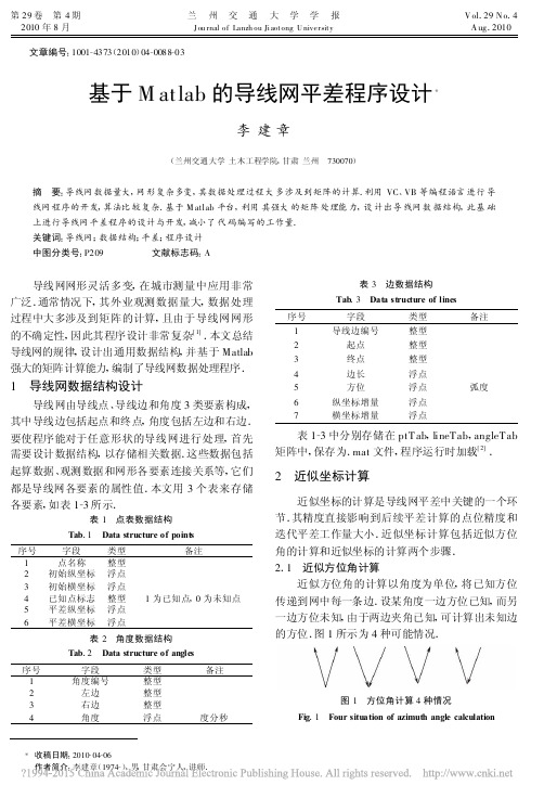
第29卷　第4期2010年8月兰州交通大学学报J ou rnal of Lanzh ou Jiaotong UniversityV ol.29N o.4A ug.2010 文章编号:1001-4373(2010)04-0088-03基于M atlab的导线网平差程序设计＊李建章(兰州交通大学土木工程学院,甘肃兰州　730070)摘　要:导线网数据量大,网形复杂多变,其数据处理过程大多涉及到矩阵的计算.利用VC、VB等编程语言进行导线网程序的开发,算法比较复杂.基于M atlab平台,利用其强大的矩阵处理能力,设计出导线网数据结构,此基础上进行导线网平差程序的设计与开发,减小了代码编写的工作量.关键词:导线网;数据结构;平差;程序设计中图分类号:P209 文献标志码:A 导线网网形灵活多变,在城市测量中应用非常广泛.通常情况下,其外业观测数据量大,数据处理过程中大多涉及到矩阵的计算,且由于导线网网形的不确定性,因此其程序设计非常复杂[1].本文总结导线网的规律,设计出通用数据结构,并基于Matlab 强大的矩阵计算能力,编制了导线网数据处理程序. 1　导线网数据结构设计导线网由导线点、导线边和角度3类要素构成,其中导线边包括起点和终点,角度包括左边和右边.要使程序能对于任意形状的导线网进行处理,首先需要设计数据结构,以存储相关数据.这些数据包括起算数据、观测数据和网形各要素连接关系等,它们都是导线网各要素的属性值.本文用3个表来存储各要素,如表1-3所示.表1　点表数据结构Tab.1　Data structure of points序号字段类型备注1点名称整型2初始纵坐标浮点3初始横坐标浮点4已知点标志整型1为已知点,0为未知点5平差纵坐标浮点6平差横坐标浮点表2　角度数据结构Tab.2　Data structure of angles序号字段类型备注1角度编号整型2左边整型3右边整型4角度浮点度分秒表3　边数据结构Tab.3　Data structure of lines序号字段类型备注1导线边编号整型2起点整型3终点整型4边长浮点5方位浮点弧度6纵坐标增量浮点7横坐标增量浮点表1-3中分别存储在ptTab,lineTab,angleTab 矩阵中,保存为.mat文件,程序运行时加载[2].2　近似坐标计算近似坐标的计算是导线网平差中关键的一个环节.其精度直接影响到后续平差计算的点位精度和迭代平差工作量大小.近似坐标计算包括近似方位角的计算和近似坐标的计算两个步骤.2.1　近似方位角计算近似方位角的计算以角度为单位,将已知方位传递到网中每一条边.设某角度一边方位已知,而另一边方位未知,由于两边夹角已知,可计算出未知边的方位.图1所示为4种可能情况.图1　方位角计算4种情况Fig.1　Four situation of azimuth angle calculation＊收稿日期:2010-04-06作者简介:李建章(1974-),男,甘肃会宁人,讲师.第4期李建章:基于M atlab 的导线网平差程序设计假定已知左边方位角为fw 1,夹角为α,则以上4种情况下右边的方位角f w r 讨论如下.情况一:fw r =fw 1+α(1)情况二:fw r =fw 1+α(2)情况三:fw r =fw 1±π+α(3)情况四:fw r =fw 1±π+α(4)同理可得,已知右边方位角计算左边方位角的情况,也有4种可能性.程序根据角度两边的端点点名的关系判断以上8种情况,采用相应的计算公式计算未知边方位角[3].程序在获得未知边方位角后,将计算结果保存到边表相应记录中.然后在角度表中搜索相邻角度,搜索条件是:该角度的一边必须是上一角度的一边,而另一边不是上一角度的一边.查询到满足条件的角度后,判断其是否为截至角(两边方位已知),如否则计算出该角度未知边方位,重复前面的步骤直至某一截至角停止.然后在边表中查询有无近似方位未知的边,如有,再次执行以上步骤,直至边表中所有边近似方位计算完毕,这个过程可以通过一个函数自身迭代来实现.程序流程如图2所示.图2　计算近似方位流程图Fig .2　Flow chart of calculating azimuth angle计算导线边方位的子程序如下所示:functio n [ptT ab ,angleT ab ,lineT ab ,ok ]=g etfw0(pt -T ab ,ang le T ab ,lineT ab )[baindex ]=getanglebeg in (angleT ab ,line Tab );%查找起算角[ok ,ptT ab ,line T ab ,ang le T ab ]=caculateFW0(baindex ,ptT ab ,line Tab ,ang le Tab );%由起算角往前传递方位.if no t (fwisok (lineTab ))%判断有没有方位未知的导线边　[ptT ab ,ang leT ab ,lineT ab ,ok ]=getfw 0(ptT ab ,a n -gleT ab ,lineT ab );　%函数迭代计算.end end2.2　近似坐标计算通过2.1计算,所有导线边的近似方位计算完毕,此时可以利用每条边的边长和近似方位计算其坐标增量,这个过程只需要在边表中循环计算即可.然后以导线边为单位,从起始边出发,将已知坐标传递到各未知点.所谓起始边即该边一端点坐标已知,另一端点坐标未知.利用导线边坐标增量计算未知点坐标,然后查找相邻边,判断其是否为截至边(两端点坐标皆知),如否,计算未知点坐标.重复查找计算直至截至边,然后程序在点表中判断有无近似坐标未知的点,如有,则重复以上步骤,否则程序退出.这个过程和2.1中计算方位角的过程是类似的,因此不再列出程序流程图和代码.3　误差方程系数矩阵计算导线网观测值有角度和边长两种类型,一个观测值可列出一个误差方程.因此程序需分别读取角度表和导线边表中每个记录来计算误差方程系数矩阵B 、常数项矩阵l 和权阵P .3.1　利用观测角度计算误差方程系数矩阵设某角度观测值为ang le ,其左边近似方位、左边长、左边起点点名,左边起点点序号,左边终点点名,左边终点点序号,左边坐标增量分别为:lfw ,ls ,lbname ,lbindex ,lename ,leindex ,ldetx ,ldety ,同理对应右边各项为:rfw ,rs ,rbname ,rbindex ,rename ,reindex ,rdetx ,rdety .由图1可知,各观测角度两边的方向有4种情况,为简化程序,首先将其全部转化为情况1.设转换后左导线边起、终点序号分别为tem lbindex ,tem -leindex .右导线边起、终序点号分别为tem rbindex ,temreindex .如下是图1第三种情况的转换代码.if lename ==rbname temlbindex =leinde x ; temleindex =lbinde x ; tem rbindex =rbindex ; tem reindex =reindex ; lde tx =(-1)＊lde tx ; lde ty =(-1)＊lde ty ; rdetx =rdetx ;89兰州交通大学学报第29卷 rdety =rdety ; lfw =lfw +pi (); rfw =rfw ;end设该角度序号为index .又左边起点、终点和右边起点、终点的未知数序号分别为:lbcontrindex ,le -contrindex ,rbco ntrindex ,recontrindex .则B (index ,(2×leco ntrindex -1))=ρΔy L 1000s 2L B (index ,(2×leco ntrindex ))=-ρΔx L1000s 2L B (index ,(2×reco ntrindex -1))=-ρΔy R1000s 2RB (index ,(2×reco ntrindex ))=-ρΔx R1000s 2RB (index ,(2×lbcontrindex -1))=ρΔy R 1000s 2R -ρΔy L1000s 2L B (index ,(2×lbcontrindex ))=-ρΔx R 1000s 2R +ρΔx L1000s 2L angle 0=r f w -l f wl (index ,1)=(angle 0-ang le )×180×3600πP (index ,index )=1[4]上述各点如为已知点,则对应系数为0.未知点序号为所有待求点的排列序号,用于控制误差方程系数在B 矩阵中的列位置.3.2　利用观测边长计算误差方程系数矩阵设某观测边坐标增量为Δx ,Δy ,观测边长为S ,S 0=Δx 2+Δy 2,则B (index ,(2×lbco ntrindex -1))=-ΔxS 0(5)B (index ,(2×lbco ntrindex ))=-ΔyS 0(6)B (index ,(2×leco ntrindex -1))=ΔxS 0(7)B (index ,(2×lecontrindex ))=ΔyS 0(8)l (index ,1)=1000×(S 0-S )(9)P (index ,index )=S100[5](10)其中已知点对应项系数为0,其中index 为观测边序号,观测边序号是该边在边表中序号加上角度观测值个数.lbcontrindex 和leco ntrindex 为该边起点、终点的未知点序号.以上过程需要一个循环语句即可完成.4　结束语本文基于Matlab 开发了导线网平差程序,算法简单,编程工作量小[6].对于测绘专业类似计算问题如三角网、水准网等的程序设计有一定的借鉴意义.由于篇幅的限制,本文没有论述其他相关处理过程的算法,包括利用误差方程迭代计算获取最优解、度分秒和弧度互化、边点要素属性的查询等,这些算法在M atlab 中实现相对比较容易.参考文献:[1]　汪自军,陈圣波,臧立娟,等.导线网数据处理系统关键技术及其实践[J ].微计算机信息,2008(2):216-218.[2]　李建章.基于M a tlab 的水准网平差程序设计[J ].兰州交通大学学报,2009,28(3):29-31.[3]　武艳强,黄立人,江在森.导线网平差中近似坐标的无限定推算方法[J ].测绘通报,2006(12):12-15.[4]　武汉大学测绘学院测量平差学科组.误差理论与测量平差基础[M ].武汉:武汉大学出版社,2003:102-125.[5]　姚德新.土木工程测量学教程[M ].北京:中国铁道出版社,2003:67-68.[6]　薄志义,曹福生.程序寻找支导线网计算路径的研究[J ].测绘科学,2007(9):68-69.Adjustment Programming of Traverse Network on the Basis of MatlabLI Jian -zhang(Sch ool of Civil En gineering ,Lanzhou Jiaotong University ,Lanzh ou 730070,China )A bstract :H aving large data and complex shape ,the data pro cessing of traverse netw o rk involves matrix cal -culation .It 's mo re difficult to prog ram on o ther prog ramming lang uages like VC and VB .In the e ssay ,the data structure o f traverse netw ork is desig ned by utilizing the matrix dispo sal capability of M atlab ,and thenthe prog ram that has the adv antag es of being simple in algo rithm is finished .Key words :trave rse ne tw ork ;data structure ;adjustment ;pro gramming90。

用MATLAB解决_条件平差和间接平差(可编辑)

用MATLAB解决_条件平差和间接平差测量程序设计条件平差和间接平差一、条件平差基本原理A LA0函数模型 A VW0r n n 1 r 1r 12 21随机模型D? Q? P0 0TV P Vm i n平差准则条件平差就是在满足r个条件方程式条件下,求使函数V‘PV最小的V值,满足此条件极值问题用拉格朗日乘法可以求出满足条件的V值。

?A LA01、平差值条件方程: 0r n n 1r 1r 1a La L a La01 12 2 n n 0b Lb L b Lb01 12 2 n n 0?r Lr L r Lr01 12 2 n n 0a ,b ,, r i1 , 2 ,, n 条件方程系数i i ia ,b ,, r0 0 0常数项?A LA02、条件方程: 0r n n 1r 1r 1将LLV代入平差值条件方程中,得到A VW0r 1 n 1 r 1 r 1w , w ,, wa b r为条件方程闭合差WA LA闭合差等于观测值减去其应有值。

3、改正数方程:按求函数条件极值的方法引入常数TK k , k ,, ka b rr 1称为联系系数向量,组成新的函数:T T? V P V2 K A VW将Ω对V求一阶导数并令其为零?T T2 V P2 K A0VT1 T TP VA K则: VP A KQ A K4、法方程: 将条件方程 AV+W0代入到改正数方程VQATK 中,则得到:TA Q A KW0N KW0记作: a ar 1 r 1 r 1r rTR N R A Q A R A r由于 a a1 T1K? N W? A Q A A LANaa为满秩方阵,a a 0TLLVVQ A K按条件平差求平差值计算步骤A VW01、列出rn-t个条件方程r 1 n 1 r 1 r 1T1 TN KW0NA Q AA P A2、组成法方程a aa ar 1 r 1 r 1r r1K? N Wa a3、求解联系系数向量4、将 K值代入改正数方程VP-1ATKQATk中,求出V值,并求出平差值LL+V。

基于MATLAB的测量平差计算

序。ＭＡＴＬＡＢ与其他算法语言相比，具有编程简单、运算速度快的特点，特别是在矩阵运算方面，在最小二乘
平差中可以发挥很好的作用，能大大提高工程测量中的数据处理效率。关键词：平差；ＭＡＴＬＡＢ优化箱；附线性不等式约束
２０１３年第７期
中州煤炭
总第２１１期
基于ＭＡＴＬＡＢ的测量平差计算
高思培，陈冠宇，范新华，王耀鑫，王强昆
（１，河南理工大学测绘与国土信息工程学院，河南焦作２．桂林理工大学测绘地理信息学院，广西桂林４５４０００；７１００４３）５４１００６；３．机械工业勘察设计研究院，陕西西安
＝
（胎）ＢＰ１，Ｐ为观测值的权阵。
平差值向量的协因数阵：
ＱＬＬ＝Ｂ（曰ＰＺ）曰
计算软件，它以矩阵运算为基础，把计算、绘图及动态系统仿真等功能有机融合在一起。ＭＡＴＬＡＢ将高性能的数值和符号计算功能、强大的绘图功能、程序语言设计功能以及为数众多的应用工具箱集成在一
Ｈａ＝２３７．４８３ｍ，为求Ｂ、Ｃ、Ｄ三点的高程，进行了水
准测量，其结果见表１，试按间接平差求定Ｂ、Ｃ、Ｄ

用MATLAB解决条件平差和间接平差

A h2 D h1
C h6 E h3 h5 h7 B h4
disp(‘C是单位权观测高差的线路公里数，S是线路长度’) 是单位权观测高差的线路公里数，是线路长度是线路长度’ 是单位权观测高差的线路公里数 C = l*ones(1,6)
S = [1.1, 1.7, 2.3, 2.7, 2.4, 4.0] P = C./S % 定义观测值的权，定义观测值的权， P = diag(P) % 定义权阵 disp(‘参数的解’) 参数的解’ 参数的解 x = inv(B’*P*B)*B’*P*l disp(‘误差误差V(mm), 各待定点的高程平差值（m）’) 各待定点的高程平差值L1（）误差 V = B*x - l % 误差方程误差方程(mm) L1 = L + V/1000 % 观测值的平差值，观测值的平差值， disp(‘精度评定’) 精度评定’ 精度评定 n = 6; % 观测值的个数 t = 2; % 必要观测数 delta = sqrt(V’*P*V/(n – t))
H(1,1)+H(2,1)-H(3,1)+HAH(2,1)if H(1,1)+H(2,1)-H(3,1)+HA-HB==0 && H(2,1)H(4,1)==0 disp(‘检核正确检核正确') disp( 检核正确') else disp(‘检核错误检核错误') disp( 检核错误') end disp(‘平差后的高程值平差后的高程值') disp( 平差后的高程值') HC = HA + H(1,1) HD = HA + H(1,1) + H(4,1)
二、间接平差的基本原理
在一个控制网中，设有t个独立参数，在一个控制网中，设有t个独立参数，将每一个观测值都表达成所选参数的函数，以此为基础进行平差，成所选参数的函数，以此为基础进行平差，最终求得参数的估计值。计值。选择参数应做到足数（参数的个数等于必要观测数）和独选择参数应做到足数（参数的个数等于必要观测数）参数间不存在函数关系）。）。利用参数将观测值表示为立（参数间不存在函数关系）。利用参数将观测值表示为

MATLAB平差程序

function BJPC2ZB=[];ZJ=[];BC=[];%%format long[filename,filepath]=uigetfile('*.txt','选择平差文件:'); name=[filepath filename];fid1=fopen(name,'rt');if(fid1==-1)disp('文件未打开，请重试！');return;endn=fscanf(fid1,'%f',1);%输入边的个数b=fscanf(fid1,'%f',1);%输入多余观测个数E=fscanf(fid1,'%f',1);%输入测角中误差t=fscanf(fid1,'%f',1);%输入坐标个数ZB=fscanf(fid1,'%f',[2 t]);dms1=fscanf(fid1,'%f',[3 n+1]);BC=fscanf(fid1,'%f',[1 n]);T0=fscanf(fid1,'%f',1);T1=fscanf(fid1,'%f',1);fclose(fid1);dms=dms1';ZJ=dms2degrees(dms);%%if t==2T0=T0;%若告诉起始方位角就直接输入endif t==4 %若没有告诉起始方位角由坐标反算Xa=ZB(1,1);Xb=ZB(1,2);Ya=ZB(2,1);Yb=ZB(2,2);Tx=Xb-Xa; Ty=Yb-Ya;T0=atan(Ty/Tx)*180/pi;%对方位角的讨论if ((Tx>0)&&(Ty>0))T0;endif (((Tx<0)&&(Ty>0))||((Tx<0)&&(Ty<0)))T0=T0+180;endif ((Tx>0)&&(Ty<0))T0=T0+360;endif ((Tx==0)&&(Ty>0))T0=90;endif ((Tx==0)&&(Ty<0))T0=270;endif((Ty==0)&&(Tx>0))T0=0;endif ((Ty==0)&&(Tx<0))T0=180;endenda0=T0;x0=ZB(1,t/2);y0=ZB(2,t/2);A=[0,0];FWJ=[];%开始计算近似方位角J=1;while(J<=n+1)belta=ZJ(J);%讨论方位角if J==1a=a0+belta;elsea=a+belta;endif a>=180a=a-180;elsea=a+180;endif a>=360a=a-360;endFWJ(J)=a;J=J+1;endFWJ;%%J=1;%开始计算近似坐标Awhile(J<=n)if J==1A(1,1)=x0+BC(1)*cos(FWJ(1)*pi/180);A(2,1)=y0+BC(1)*sin(FWJ(1)*pi/180);elseA(1,J)=A(1,J-1)+BC(J)*cos(FWJ(J)*pi/180); A(2,J)=A(2,J-1)+BC(J)*sin(FWJ(J)*pi/180);endJ=J+1;endA;%%W=[];%开始计算闭合差if t==2T1=T1;endif t==4Xa=ZB(1,3);Xb=ZB(1,4);Ya=ZB(2,3);Yb=ZB(2,4);Tx=Xb-Xa; Ty=Yb-Ya;T1=atan(Ty/Tx)*180/pi;if ((Tx>0)&&(Ty>0))T1;endif (((Tx<0)&&(Ty>0))||((Tx<0)&&(Ty<0)))T1=T1+180;endif ((Tx>0)&&(Ty<0))T1=T1+360;endif ((Tx==0)&&(Ty>0))T1=90;endif ((Tx==0)&&(Ty<0))T1=270;endif((Ty==0)&&(Tx>0))T1=0;endif ((Ty==0)&&(Tx<0))T1=180;endendW(1,1)=-(FWJ(n+1)-T1)*3600;%以秒为单位W(2,1)=-(A(1,n)-ZB(1,t/2+1))*100;%以厘米为单位W(3,1)=-(A(2,n)-ZB(2,t/2+1))*100;W;%%XS=zeros(3,2*n+1);%开始计算系数阵，XS是系数阵e=n+1;while(e<=2*n+1)XS(1,e)=1;e=e+1;endf=1;while(f<=n)XS(2,f)=cos(FWJ(f)*pi/180);%纵坐标边长改正数的系数 XS(3,f)=sin(FWJ(f)*pi/180);%横坐标边长改正数的系数 f=f+1;endu=1;y0=A(2,n);x0=A(1,n);Y=[];X=[];y1=[];x1=[];while(u<=n+1)if u==1Y(1)=ZB(2,t/2);X(1)=ZB(1,t/2);elseY(u)=A(2,u-1);X(u)=A(1,u-1);endu=u+1;endy1=-1/2062.65*(y0-Y);%纵坐标转角改正数的系数x1=1/2062.65*(x0-X);%横坐标转角改正数的系数y1;x1;d=n+1;z=1;while(d<=2*n+1)XS(2,d)=y1(1,z);XS(3,d)=x1(1,z);d=d+1;z=z+1;endXS;%%r=[];h=1;while (h<=n)s=(5+5*BC(h)/1000)/10;%求中误差厘米为单位r(h)=E^2/s^2;%计算距离的权h=h+1;endaa=[];y=1;while(y<=n)aa(y)=r(y);%将距离的权赋给矩阵aay=y+1;endc=n+1;while(c<=2*n+1)aa(c)=1;%转角的权都是1c=c+1;endP=diag(aa);%形成权阵P;%%Q=inv(P);N=XS*Q*XS';N1=inv(N);K=inv(N)*W;V=Q*XS'*K;V;BC1=BC'+V(1:n)/100;%将改正数加到观测值以求平差边长（除一百统一单位）ZJ1=ZJ+V(n+1:2*n+1)/3600;%同上BC1;i=1;while (i<=n+1)ZJ2(i,1)=fix(ZJ(i));ZJ2(i,2)=fix((ZJ(i)-fix(ZJ(i)))*60);ZJ2(i,3)=((ZJ(i)-fix(ZJ(i)))*60-fix((ZJ(i)-fix(ZJ(i)))*60))*60;i=i+1;endZJ2;%%A1=[0,0];FWJ1=[];J=1;while(J<=n+1)belta=ZJ1(J);if J==1a=a0+belta;elsea=a+belta;endif a>=180a=a-180;elsea=a+180;endif a>=360a=a-360;endFWJ1(J)=a;J=J+1;endi=1;while (i<=n+1)FWJ3(i,1)=fix(FWJ(i));FWJ3(i,2)=fix((FWJ(i)-fix(FWJ(i)))*60);FWJ3(i,3)=((FWJ(i)-fix(FWJ(i)))*60-fix((FWJ(i)-fix(FWJ(i)))*60))*60;FWJ2(i,1)=fix(FWJ1(i));FWJ2(i,2)=fix((FWJ1(i)-fix(FWJ1(i)))*60);FWJ2(i,3)=((FWJ1(i)-fix(FWJ1(i)))*60-fix((FWJ1(i)-fix(FWJ1(i)))*60))*60; i=i+1;endFWJ3;FWJ2;%%J=1;%开始计算平差坐标A1while(J<=n)if J==1A1(1,1)=ZB(1,t/2)+BC1(1)*cos(FWJ1(1)*pi/180);A1(2,1)=ZB(2,t/2)+BC1(1)*sin(FWJ1(1)*pi/180);elseA1(1,J)=A1(1,J-1)+BC1(J)*cos(FWJ1(J)*pi/180);A1(2,J)=A1(2,J-1)+BC1(J)*sin(FWJ1(J)*pi/180);endJ=J+1;endA1;m=sqrt(V'*P*V/b);%测量精度单位权中误差。

学位论文—基于matlab测量平差程序设计-创新实践报告

创新实践报告实践名称：基于MATLAB测量平差程序设计系部名称：测绘工程学院专业班级：测绘工程11-6班学生姓名：学号：指导教师：xxx工程学院教务处制注：1、此报告为参考格式，各栏项目可根据实际情况进行调整；实验成绩以优（90~100）、良（80~89）、中（70~79）、及格（60~69）、不及格（60以下）五个等级评定。

附录1 外文参考文献原文参考文献一Improving oil fields recovery through real-time water flooding optimizationPamela Alessia Chiara MarescalcoPolitecnico di Torino, Land, Environment and GeoTechnologies Engineering Department,24, C.so Duca degli Abruzzi, 10129 Torino, ItalySUMMARYIncreasing oil recovery from reservoirs is a strong urge. One of the most effective ways to get the result iswater flooding and that’s why its application is nowadays widely used in the petroleum industry. Obviously,water flooding efficiency strongly depends on reservoir properties; this makes simulating a water injectionprocess a priori an extremely important step of the reservoir production strategy. Simulation is commonlydone adopting a finite difference (FD) simulation approach.This paper explores a different and complementary approach, represented by streamline-based simulation,coupled with a tool to optimize water flooding campaigns and to help quick decision making. Inthe present study, water flooding simulation is performed via two commercial software: an FD and astreamline-based simulator, to highlight advantages and disadvantages of both simulation techniques indescribing a water injection campaign and to exploit the two appr oaches’ uniqueness in parallel.The final goal of iteratively converging to the optimal water flooding scheme, which is the core of thepresent work, is achieved through a customized Matlab script. The generated automatic procedure showsits effectiveness in improving oil recovery, expediting decision making and saving time and FD simulationruns. A three steps workflow is outlined to get the best water flooding scheme for the examples shownbelow. Copyright q 2008 John Wiley & Sons, Ltd.Received 13 March 2008; Revised 1 September 2008; Accepted 8 November 2008KEY WORDS: water displacement optimization; FD simulation; streamline simulation; Matlab automatedroutine; real-time decision making; quantitative and iterative adjustment of water rates tobe injectedINTRODUCTIONIn the last decades water flooding has been widely applied in the petroleum field, both in mature and in newly developed fields, and its attractiveness lies in supporting the entire field pressureduring depletion and in improving the final oil recovery [1–3]. The techniqueconsists in injecting water with the purpose of displacing and therefore producing oil, especially if the reservoir lacks an underlying aquifer able to counterbalance the depletion and to drive oil to the producer wells.To really understand a water flooding process and to predict its efficiency, it is useful to simulate it a priori. This is usually done via finite difference (FD) simulation, which is able to describe any kind of existing reservoir very accurately, but unfortunately is not able to give enough details about the way the flow occurs throughout the field. Recent works [4, 5] have proposed a newly developed approach, based on streamline simulation, whose main attraction lies in providing information not obtainable from FD simulation and useful for the purpose of improving reservoir performances.In the present study, water flooding simulation is performed via two commercial software: an FDand a streamline-based simulator, to highlight advantages and disadvantages of both simulationtechniques in describing a water injection campaign and to exploit the two approaches’ uniquenessin parallel. If FD simulation is essential to checking the streamline simulation results, the streamlinebasedsimulator is, on the other hand, an ideal tool to perform a procedure able to optimizewater injection. Then, the core of the work and its innovative approach lies in exploiting the twosoftware features in conjunction with the application of a customized Matlab code developed inorder to elaborate all the streamline simulation outputs, to calculate the changes to be made to theproduction/injection constraints for the subsequent simulation run, so as to iteratively converge tothe optimal injection scheme for the reservoir under study. A three steps workflow is outlined toget the best water flooding scheme for the examples shown below.FD APPROACH VERSUS STREAMLINE SIMULATIONECLIPSE is a complete and complex simulator, whose attractiveness resides in being able todescribe any kind of reservoir, including geological complexity, formation features, and fluidproperties. The simulator is based on a time and spatial discretization and solves a three-dimensionalequation by assigning to all the parameters involved in the simulation a unique value, associated withthe entire cell, for every grid block. For models with a large number of cells, using FD relaxationcan be computationally heavy; therefore, a good balance must be kept between having sufficientaccuracy in describing the reservoir and keeping simulation time within reasonable limits [6].3DSL, on the other side, solves two different equations on two different grids and this is usuallyfaster than FD simulation, especially for large models: the pressure equation is solved implicitlyon the background grid (or pressure grid), whereas the saturation equation is solved explicitly onthe streamline grid. This involves a minor effect of grid refinement on the resultsof the simulation,time-step limitations not as severe, thanks to a better stability of the geometrical grid, numericaldiffusion easier to control, faster solutions with respect to FD approach [7].Streamline simulation solves mono-dimensional equations along streamlines, which means itsolves multiple streamlines in parallel, and the fluid transport, which for FD approach occursbetween grid cells [8], occurs along streamlines: this gives an immediate answer in terms of howthe streamlines (connecting injector and producer wells—to say, well pairs) are distributed, sothat the fluid trajectories and their rates at the wells are known at every time step [9, 10]. Thanksto the available information, the distribution of injected water volumes can be modified, and amore effective production strategy can be planned to maximize oil recovery [4, 5]. Same as for FDsimulation, when using streamline-based simulation a good balance must be maintained betweenpressure updates and computational speed.In conclusion, 3DSL is simpler from a reservoir description (includes both flow physics andpetro-physical/geological information) point of view, but it cannot take into account importantparameters such as capillary pressure or cross flow effects: moreover, fluid compressibility cannot beeasily taken into account and mass conservation errors may occur while mapping between pressuregrid and streamline grid therefore being incomplete or inadequate for most of real reservoirs. Everyfurther detail can be found in previous works [11]. THE IDEA OF THE STUDYIn this paper the use of the two software as complementary tools to optimize water injectionis shown: ECLIPSE appeared to be the most reliable software to simulate reservoir models andto be essential to verify 3DSL’s results accuracy upstream and downstream of the methodologydeveloped for this research, while 3DSL has been shown to be simpler and usually faster, providinginformation not obtainable by means of FD simulation, and which could be exploited to save atrial-and-error process trying to find the best injection schemeThe idea of the study resulted from previous works [12].The research presented here follows a three step workflow. In the first part of the study, thetwo software were used to simulate simple synthetic models. Once the results obtained from thetwo simulators were checked for consistency, a method was developed to exploit 3DSL’s features.The most interesting pieces of information available from 3DSL are the connections between wellpairs (injector-producer) and the rates at the wells and the connections. With this informatioavailable, the streamline simulator, coupled with Matlab, was involved into an automatic procedurethat reallocated water injected volumes in order to optimize water injection campaigns, for all the examined cases.This was gained by a customized Matlab script, writtenfor this specific purpose, which automaticallyinteracted with the streamline simulator, processed the input data supplied by the softwaregiving back new input rates to be used for the following simulation run. This was done for a fixednumber of runs to iteratively converge to the optimal injection scheme. From preliminary analyses[13] the procedure was shown to be effectiveEventually, in the third experimental phase, the last rates calculated from Matlab were inputinto ECLIPSE to check the procedure’s effectiveness and the added val ue in terms of oil recoveryimprovement.THE AUTOMATED PROCEDURE AND THE EXPERIMENTAL METHOD Let’s now focus on the second and main part of the experimental study which, as we said, consistedin writing a customized Matlab code. Streamline answers in terms of streamlines distribution(connecting injector and producer wells—or well pairs) and fluid rates at the wells are writtenat every time step in a 3DSL output file named ∗.WAF, which is crucial for the entire codingdescribed below and for its application.The endeavor of the Matlab customized code is the optimization of the displacement processthrough a gradual reallocation of injected water rates, carried out by increasing the water volumeinjected at the highly efficient connections and decreasing it at the poorly efficient connections.The term injection efficiency (for a well pair connection) stands for the ratio between offset oilproduced thanks to water displacement and the amount of water injected at a certain well. In ananalogue manner the injection efficiency of an injector well is the ratio between offset oil at allproducers connected to it and the total water injected at the same well. The approach used forthe current application was aimed at increasing the oil production through a better use of a givenwater volume available for injection. The Matlab code written for this purpose mainly works asfollows: the data needed for the procedure are read from 3DSL’s output ∗.WAF file and loadedinto Matlab environment, then they are processed throughout the code; eventually new rates forthe next simulation run are output to 3DSL. This is all done automatically with an approach aimedat maximizing oil production through a more efficient use of a given water volume available forthe injection [13]. The code steps are here summarized [12]:1st step consists in: establishing the number of iterations to be run for the procedure of ratereallocation and their duration; fixing the volume of water to be injected and the target liquid rate.2nd step consists in: running a ‘do nothing’ 3DSL simulation in order to choose a properstarting time for the entire procedure of rate reallocation (usually the reallocation startswhereas aproduction plateau starts).3rd step consists in: reading (within the Matlab environment, by means of functions coded onpurpose) from the ∗.WAF file: rates (total rate for each injector well, and partial rate for eachproduction well connected to the injector); time; name and number of injector or producer wellsand connections between them; number of existing connections in the model at any time step ofthe simulation.4th step consists in: calculating the injection efficiency for each well pair, for each injector well,and for the field (average injection efficiency).5th step consists in: calculating for each iteration and for each injector well a new rate:Qnew i=(1+wi )·qoldi (1)where i stands for the well, wi for the weight it has been assigned, and qoldi for the rate injectedat the well at the previous step.The average reference field injection efficiency (referred to as signed e) is a mean value:depending on its value, positive or negative weights are assigned to the efficient or inefficient connections.Once the maximum weight, minimum weight, minimum injection efficiency allowed, maximum injection efficiency awaited, and _ (which is the grade of the polynomial that interpolates the relation weight-efficiency) are fixed, the weights are evaluated as follows:where wmin is the minimum weight at the least efficiency, wmax is the maximum weight at thehighest efficiency, emin is the least acceptable injection efficiency, emax is the highest awaitedinjection efficiency.6th step consists in: calculating new rates for each well pair connection and, consequently, foreach injector; calculating for each injector the differences between the last known rates and thenew ones; determining the new total volume of water injected as a summation of the new rates atthe injectors; checking that the constraints on the total water volume available (x) are satisfied byFigure 1. Weighting functions (as from Equations (2) and (3)) for different values of exponent_.introducing a correction factor c:c=_x qnew i(4)7th step consists in: calculating new liquid rates (for each producing well the novel rate iscalculated by adding/subtracting the same amounts of water rate, _q±, calculated for the injectorwells connected to it), imposing that the constraints on the total liquid volume (y) are satisfiedthrough the correction factor c1:c1= _y qnew i(5)8th step consists in: making Matlab write a text file to be included in the 3DSL dataset,summarizing all the new rates and time information.9th step consists in: running the reallocation procedure, following the eight steps listed above,for as many iterations as initially fixed (well rates and time are updated at every _t).Both _t and the set of parameters chosen at the 5th step affect the final results.For all the examples shown here, to signed e was allotted the average field efficiency value, inorder to have a case sensitive value. At the same time, _ was put equal to 2 for all the exam inedcases, so that the weighting function would be nonlinear and the most significant changes in injection rates would occur far-off from the average efficiency, while only small changes would take place around the mean value (Figure 1).For the examples shown below, parameter sensitivities were performed in order to get the bestset for the application of the Matlab code.RESERVOIR MODELS DESCRIPTIONIn this paper two synthetic models and a real one are presented.The numbers of cells for the synthetic models are 20×20×1 for the first case, and 123×54×1for the second case. A uniform discretization of the volume was chosen to accurately describe the phases present in both models are water and oil, which is supposed to be dead oil. Both water and oil have the same viscosity, equal to 1 cp. Oil and water density are, respectively, 780 and1029kg/m3. Datum pressure is equal to 30 bars. For both models, water and liquid constraints are set equal, to let the displacement occur by voidagereplacement, and correspond to 80.000rm3/day and to 150.000rm3/day, respectively. For both models the reallocation procedure starts at day 730;the number of steps, whose duration is 730 days each, is equal to 10.Similarly a real field was tested. The model was available from ECLIPSE; a translation work was done to obtain a model written for 3DSL. The two models were then checked to verify the coherence of the main parameters. Once the match was gained, 3DSL model was used to apply the procedure. The real model, as shown in Figure 4(a, b), is divided into three regions by the presence of faultsFigure 4. (a) Faults divide model three into three regions and (b) model three has three different regions.Figure 5. Permeability (a) and porosity map (b). Model three.The number of cells is 68×71×23. The grid cells are not uniform. Permeability and porosity arehighly heterogeneous and range from 0 to 1315mD and from 4 to 27%, respectively (Figure 5(a, b)).The other model properties are summarized in Tables I and II.Table II. Model three: main parameters.Swi (three regions) 0.13; 0.29; 0.06RESULTSThe three models examined were all used for the three steps workflow related before.First of all, the match and coherence between the two models were always obtained. At thispoint no relevant discrepancies were observed between the two sets of results for thethree models.Figure 6(a, b) shows, respectively, oil and water cumulative production from the third model only,as an example.At a second stage, Matlab code was applied to each 3DSL model, starting from a certain moment in time, fixed at day 730 for all the three examples. Ten iterations were run, each of them lasting730 days, and the total time for the procedure to run was fixed so as to be compared with the base case ‘do nothing’ simulation run.As for the frequency of the injection update, the longer the time step is, the higher the rates injected/produced and the major the changes concerning the values of well pairs injection efficiencies during the time steps. For the present work the well pairs injection efficiencies were assumed to remain constant throughout the single time step. Shorter time steps would maybe more suitable to this hypothesis but, on the other hand, they would imply a much higher computational time. In a real field application it might be useful to try with medium time steps (i.e. 6 months),eventually shortening them if, by analyzing the real-time field data, an intervention would appear to be needed.Each model was then compared with its respective optimized case, as shown in Figures 7–9(a, b).The figures again show, respectively, oil and water cumulative production from the field for the three models in sequence. For all the models the generated methodology was shown to give good results and to carry advantages with respect to the mere base case.The two synthetic cases showed good results both in terms of a relevant improvement in oil recovery and of a significant reduction in water production (the results are summarized in Tables III–V). Figure 10(a, b) shows the displacement of model two at the end of the simulation,for the base case and for the reallocated rates case, respectively.The real case, which at the time of this research was a pure forecast example, since the reservoir was not producing, so no production history was available, showed to gain a certain amount of oil production, but in parallel a higher water production.At the third stage the final rates observed from the 3DSL ‘optimized’ case were input in ECLIPSE, to double check the effectiveness of the optimization for the specific case. Figure 11(a, b)P. A. C. MARESCALCOFigure 6. Match ECLIPSE versus 3DSL: oil (a) and water cumulative production (b). Model three.Figure 7. Base case versus reallocated rates case: oil (a) and watercumulative production (b). Model one.Figure 8. Base case versus reallocated rates case: oil (a) and watercumulative production (b). Model two.RECOVERY THROUGH REAL-TIME WATER FLOODING OPTIMIZATIONFigure 9. Base case versus reallocated rates case: oil (a) and water cumulative production (b). Model three shows oil and water cumulative production for the second synthetic model, obtained with ECLIPSE before and after the reallocation procedure.For the synthetic models, whose ECLIPSE results downstream of Matlab procedure are as good as expected, the methodology proved to be valid.Figure 10. Oil displaced at the end of the simulation run: base case(a) and reallocated rates case (b). Model two.Figure 11. Reallocated rates case versus base case, ECLIPSE check simulation run, oil(a) and water cumulative production (b). Model two As for the real case, the results at this stage are not as good as expected. In the next paragrapha few comments on this will be remarked.DISCUSSION AND CONCLUSIONSLooking at the results, it can be generally said that the Matlab code written for this study has added value to the reallocation procedure, making it reliable and attractive for itsapplication in the petroleum industry. Previous works [12] conducted for fields under production and the two simpler examples reported here undoubtedly proved that reallocating water to optimize waterinjection is effective both for models with simpler reservoir features (incompressible fluids, simple geology) and for more complex cases (compressible fluids, heterogeneous formation): an in creased oil production was observed together with a reduced water production.As stated in the previous paragraph, for the real model, the optimized case with respect tothe base case shows a good improvement in oil recovery, but a parallel higher water production:the field in fact had not yet been deployed, so no real-time production neither geological no rpetrophysical information was provided. The reservoir features and the specific values assigned to the main reservoir parameters were then simply estimated: the values assigned to model parameters were a choice among other equally valid assessments. Last but not the least, ECLIPSE’s results certainly depend on the large amount of modifications done with respect to the original ECLIPSE model, modification necessary in order to comply with 3DSL’s binding simplifying hypotheses at the time the model ‘translation’ was doneThe aim of the research work of developing a completely automatic procedure to find the best scheme for the volumes to be injected and of using 3DSL coupled with Matlab and ECLIPSE as complementary tools proved to be effective and valid. The entire work represents a real help when a quick decision on a water flooding arrangement has to be made, both for injection campaigns yet to plan or for injection operations to be adjusted.If a reallocation procedure was to be performed only by means of ECLIPSE, a trial-and-error procedure would be needed, with a considerable waste of computational time and simulation runs.On the other hand, 3DSL allows for more simulations in parallel, saving computational time and redundant simulations.The present research in the future can be extended to a real case with a known production history to calibrate the best injection scheme.附录2 外文参考文献翻译提高油田采收率通过实时水驱优化帕米拉·阿卢嘉勒都灵理工大学摘要：提高油藏的采收率是强烈的欲望。

基于MATLAB的单三角锁严密平差程序设计

一
ｉｓ＝；０＝ｌ％当待定点为第奇数个时，待ｌ＝ｅｏ（；ＯｚｒｓＯ）ｒｏ＝：ｆｒｉｌＨ定点近似坐标的求法；３ｘ（（１ｃｔ１２＂ｘ一）ｃｔ１２＂ｙｆｒｊ１；ｘ￣ｉ）ｏ（－，＋Ｏ２ｏ（一， — ｏ＝：ｉ一ｄ（１ｉｄ（３－ｉａ１ｙ— ）一）＇＋；ｉｌｊ０ｆＯ）＝＞ｆ）ｃｔ（２）ｃｔａ２肛￣＝ｏ０－，— ｏ０一 ’ ｉｄｉ１－ｄ３１，１（）０ｊ０ｉ；６）０，＝ｊｅｓｌｅｙ＝０１ｃｔ１２＂ｙ —）ｏ０－３））一）ｏ（一，＋６２ｃｔ６２）ｘ－ｄ（ｌｙｉｄ＋
⑤计算法方程式的系数及权的编程如下：
ｌ＝２６６．０６４０６；３０；ｏ０２４８２７９４Ａ＝６０，
“ ２＋１＿）一ｆｉｃｔ（－，）ｃｔＯｉ２）ｆ￣ｏｄ１２）ｏｄ（，）（＝（３＋ｉ－１：ｙ（ｙ一）ｏ（一’ ａ１ｃｔｏ２ ” ｙ＝（２ｃｔ１２ｙ— ）ｏ０一，＋ｉｉｄ（３）ｉｄ１（２－（１ｉ）－ｉ）－ｘ一；列出误差方程＝ —ｆ；ｘ－ｘ）（（ｘ（ｆ）ｉｉｆ）／ｉ（）由误差方程系数Ｂ和自由项ｌ３组成法ｙ）ｙ（ｆｉ（ｙ）ｆｉｉ（－／）ｅｄｎ方程Ｎ — ：Ｗ０，法方程个数等于参数的个数ｔ；ｅｄｎ
Ｂ＝ｅｏ０ｎｎ２；Ｙｚｒ＊，（）ｓ２＋）始化矩阵Ｂ；Ｙ

用MATLAB解决-条件平差和间接平差

B L2
L1 A
L3 C
9
clc Disp(‘条件平差示例２’) Disp(‘三角形内角观测值’) L1 = [42 12 20] L2 = [78 9 9] L3 = [59 38 40] L = [L1; L2; L3] Disp(‘将角度单位由度分秒转换为弧度’) LL = dms2rad(mat2dms(L))
设误差Δ和参数X的估计值分别为V 和 Xˆ
15
则有
V AXˆ l
为了便于计算，通常给参数估计一个充分接近的近似值 X 0
Xˆ X 0 xˆ 则误差方程表示为
V Axˆ l
其中常数项为
l L (AX 0 d)
16
由最小二乘准则，所求参数的改正数应该满足
V T PV min
目标函数对x求一阶导数，并令其为零
if(sum(LL) == pi) disp(‘检核正确’)
else
V = A'*Ka
disp(‘检核错误’) end
11 例《误差理论与测量平差基础》P75
在下图中，Ａ、Ｂ为已知水准点，其高程为 HA=12.013m, HB = 10.013m, 可视为无误差。为了确定点Ｃ及Ｄ点的高程，共观测了四个高差，高差观测值及相应的水准路线的距离为：
disp(‘系数矩阵B’)
B = [1 0; 0 1; 1 0; 0 1; -1 1; -1 0]
l = [0; 0; 4; 3; 7; 2]
disp(‘C是单位权观测高差的线路公里数，S是线路长度’)
C = l*ones(1,6)
23
h6
E h3
h7 B
S = [1.1, 1.7, 2.3, 2.7, 2.4, 4.0]

1、下载文档前请自行甄别文档内容的完整性，平台不提供额外的编辑、内容补充、找答案等附加服务。
2、"仅部分预览"的文档,不可在线预览部分如存在完整性等问题,可反馈申请退款(可完整预览的文档不适用该条件!)。
3、如文档侵犯您的权益，请联系客服反馈,我们会尽快为您处理(人工客服工作时间：9:00-18:30)。

基于MATLAB的水准网和测边网平差程序设计摘要MATLAB是目前在研究机构广泛应用的一种数值计算及图形工具软件，它的特点是语法结构简明、数值计算高效、图形功能完备，特别适合非专业编程员完成数值计算、科学试验处理等任务。

以往的测量数据处理方法需要编制特定的处理矩阵运算程序，而且程度复杂，难度大。

本文介绍一种基于MATLAB的水准网和测边网的程序设计方法，与其它算法语言相比，具有编程简单，运算速度快的特点。

文中分别阐述了水准网和测边网程序的理论基础、实现步骤和运行结果。

通过实例的分析，总结出利用MATLAB对测量数据处理有很大的应用价值，它缩短了编程的时间，提高工作效率。

关键词：MATLAB；水准网；测边网；程序设计ABSTRAC TMATLAB is one species of numerical-values calculation and graphic tools software which is widely used to apply at research institutions at present. The particularities are: concise grammar-structure、highly efficient in numerical values calculating、complete function of graphs、especially it is adapted to evildoing professional programmer to accomplish the tasks that are numerical-values calculating and scientific experiments treating. The ancient methods of measured data-processing need establishing special proceedings of treating matrices operation, moreover, it is complex and greatly difficult.This article introduces one programming method dealing with leveling and measuring edge network based on MATLAB. Compared with other algorithm language, it has particularities which are simply programming and quickly operating. The article separately expatiate the theories basics、realizing steps and running results at leveling and measuring edge network. With the analysis of examples, it has prodigious application value in measured data-processing by use of MATLAB. Moreover, it shortens programming time and improves working effectiveness.Key words：MATLAB；leveling network；measuring edge network；programming毕业设计目录目录绪论 (4)1. MATLAB软件简介 (5)2．MATLAB 在测量平差中的应用 (6)2.1测量平差原理的概述 (6)2.2平差程序总体方案 (7)3.水准网平差程序 (8)3.1程序的功能 (8)3.2水准模型网的间接平差 (8)3.2.1 “权”值的确定 (8)3.2.2 水准路线的平差计算 (9)3.2.3 精度评定 (11)3.3水准网间接平差程序信息设计 (11)3.4 水准网程序与使用说明 (12)3.4.1 水准网程序流程图 (12)3.4.2 水准网程序的使用 (12)3.5案例 (13)4. 测边网平差程序设计 (15)4.1数学模型 (15)4.1.1 误差方程和法方程的组成 (15)4.1.2 边长观测的权 (15)4.1.3 解算法方程 (16)4.1.4 精度评定 (19)4.2 测边网平差信息设计 (20)4.2.1 主要的技术要求 (21)4．3利用MATLAB的绘图语句绘制网图 (21)4.4测边网程序和使用说明 (22)4.5 程序代码说明： (23)4.6程序的使用算例 (25)结论 (29)致谢 (30)参考文献 (31)附录一 (32)附录二 (36)附录三 (46)东华理工大学毕业设计绪论绪论作为一名测量技术人员，如果不掌握一门PC机编程语言与便携计算工具，要想提高测量工作的效率几乎寸步难行。

测量需求的多样性与复杂性，造就了测量计算鲜明的个性化特点，这就是在商业测量计算软件高度发达的今天，掌握一种实用的程序语言进行编程计算仍有广泛的市场需求的重要原因。

当今较流行的计算机程序语言基本上都是基于Windows的，例如Turbo Pascal,Visual Basic,Visual C,Borland C++等，这些程序语言的优势是基于对象及可利用Windows丰富的系统资源，应用它们可以开发出界面非常丰富和友好的应用程序，其劣势主要有以下几点：1.Windows程序都非常庞大，学习并熟练掌握它们并非易事。

2.虽然市场上已有的多种专用的测量平差软件都是采用C语言开发的，但这些软件价格都比较贵，而且都带有加密狗，一次只能供一个用户使用。

出于商业目的，开发商不会公开程序源代码，这为修改程序功能以适应用户的特殊需求带来了不便。

3.在测量生产中，经常需要根据工程的实际情况进行一些个性化的数值计算工作，这些数值计算工作无固定模式，这就需要求测量技术人员最好能熟练掌握一种适用于数值计算的程序语言，以便提高测量计算的效率。

4.C语言的数值计算语句不够丰富，例如，在测量平差计算中，经常需要进行的矩阵运算，尤其是解法方程的矩阵求逆不能直接使用语句实现，而必须应用计算机算法编程实现。

如果不是基于商业软件开发，只为满足实际测量工作计算需要，则C语言的劣势就变成了MATLAB语言的优势。

东华理大学毕业设计MATLAB软件简介1. MATLAB软件简介MATLAB是从Matrix(矩阵)和Laboratory(实验室)各取前3个字母组成的,意思是矩阵实验室,是美国MathWorks公司于20世纪80年代中期推出的一种交互式、面向对象的科技应用软件,是一个为科学和工程计算而专门设计的高级交互式软件包。

MATLAB 集成了图示与精确的数值计算,是一个可以完成各种计算和数据可视化的强有力工具,其优秀的数值计算能力和卓越的数据可视化能力使其很快在数学软件中脱颖而出,成为以矩阵运算为主要工作方式的线性代数、概率论和数理统计、自动控制、数字信号处理、动态系统仿真等领域教学和科研工作者的有力武器。

随着该软件自身的发展及市场的需求,其功能日趋完善,其最高版本7.0版已经推出,随着版本的不断升级,它的数值计算及符号计算功能得到了进一步完善。

MATLAB是以矩阵作为数据操作的基本单位,矩阵的生成、运算、转置、求逆等非常简单。

在MATLAB环境中,不需要对创建的变量对象给出类型说明和维数,所有的变量都作为双精度数来分配内存空间,MATLAB将自动地为每一个变量分配内存。

MATLAB语言起源于矩阵运算,并已经发展成为一种高度集成的计算机语言,它提供了强大的科学运算、灵活的程序设计流程、高质量的图形可视化与界面设计、便捷的与其他程序和语言接口的功能。

MATLAB系统主要包含5 部分的内容:MATLAB 工作环境、Mablab 数学函数库、MATLAB语言体系、句柄图形、MATLAB应用程序接口(API)。

MATLAB系统主要功能包括:数值计算功能、符号计算功能、数据分析和可视化、文字处理功能、SIMULINK动态仿真功能。

同时,MATLAB又是开放的,除了内部函数之外,所有的MATLAB 主包文件和各工具包文件都是可读可改的源文件,用户可以作为参考掌握其用法,并可对其修改以适应自己的需要,也可加入自己编写的文件构成新的工具包。

例如,随着GPS 的广泛应用,Orion Dynamics and Con2t rol Corporation、Constell Inc. GPSSoft LLC、NavsysCorporation等多家公司都相应开发出了适于GPS数据处理的MATLAB 工具箱。

MATLAB是一个集数值计算、图形管理、程序开发于一体的功能十分强大的系统。

将MATLAB应用于测量数据的处理是一件非常有意义的工作。

Mo2hamed等曾成功地在MATLAB系统中利用白滤波技术研究动态解算GPS载波相位信号的模糊度问题。

因为测量数据的处理特别是测量平差主要应用矩阵运算,而MATLAB又特别易于做矩阵运算,因此,研究开发基于MATLAB的测量平差方法具有极好的应用价值。

2．MATLAB 在测量平差中的应用测量平差数据处理主要是基于矩阵的运算,常用的矩阵运算主要是矩阵的生成、转置、求逆和矩阵求广义逆等。

在MATLAB 环境中,不需要对创建的变量对象给出类型说明和维数,所有的变量都作为MATLAB 中的M 文件的语法与其他的高级语言类似,是一种程序化的编程语言,同时也是一种解释性的编程语言,即逐行解释运行程序,使程序容易调试,计算更为简捷,而且对于平差原理理解和掌握变得更容易。

另外,MATLAB 语言与数学语言比较接近,更容易掌握和理解。

2.1测量平差原理的概述测量平差的函数模型有条件方程和观测方程。

以条件方程为函数的模型的最小二乘平差称为条件平差；在条件方程中，根据需要如果还设有一定数量的未知数，则称为附有参数的条件平差；以观测方程为函数模型的最小二乘平差称为间接平差；如果观测方程中的某些参数不独立，则这些不独立参数必然存在一些条件，称这种平差模型为附有条件的间接平差。

本文的两个程序都采用间接平差模型。

对于一个实际平差问题,根据所选参数的个数、选什么量为参数以及参数之间是否函数独立,经过仔细推敲可以发现附有条件的间接平差模型本身就是各种经典平差模型的概括模型,其余的经典平差模型,如条件平差模型、间接平差模型、附有未知数的条件平差模型和附有限制条件的条件平差模型都是它的特例。