Calogero Models for Distinguishable Particles

合集下载

英语

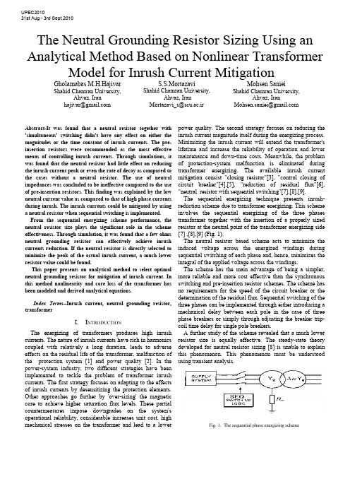
The Neutral Grounding Resistor Sizing Using an Analytical Method Based on Nonlinear Transformer Model for Inrush Current MitigationGholamabas M.H.Hajivar Shahid Chamran University,Ahvaz, Iranhajivar@S.S.MortazaviShahid Chamran University,Ahvaz, IranMortazavi_s@scu.ac.irMohsen SanieiShahid Chamran University,Ahvaz, IranMohsen.saniei@Abstract-It was found that a neutral resistor together with 'simultaneous' switching didn't have any effect on either the magnitudes or the time constant of inrush currents. The pre-insertion resistors were recommended as the most effective means of controlling inrush currents. Through simulations, it was found that the neutral resistor had little effect on reducing the inrush current peak or even the rate of decay as compared to the cases without a neutral resistor. The use of neutral impedances was concluded to be ineffective compared to the use of pre-insertion resistors. This finding was explained by the low neutral current value as compared to that of high phase currents during inrush. The inrush currents could be mitigated by using a neutral resistor when sequential switching is implemented. From the sequential energizing scheme performance, the neutral resistor size plays the significant role in the scheme effectiveness. Through simulation, it was found that a few ohms neutral grounding resistor can effectively achieve inrush currents reduction. If the neutral resistor is directly selected to minimize the peak of the actual inrush current, a much lower resistor value could be found.This paper presents an analytical method to select optimal neutral grounding resistor for mitigation of inrush current. In this method nonlinearity and core loss of the transformer has been modeled and derived analytical equations.Index Terms--Inrush current, neutral grounding resistor, transformerI.I NTRODUCTIONThe energizing of transformers produces high inrush currents. The nature of inrush currents have rich in harmonics coupled with relatively a long duration, leads to adverse effects on the residual life of the transformer, malfunction of the protection system [1] and power quality [2]. In the power-system industry, two different strategies have been implemented to tackle the problem of transformer inrush currents. The first strategy focuses on adapting to the effects of inrush currents by desensitizing the protection elements. Other approaches go further by 'over-sizing' the magnetic core to achieve higher saturation flux levels. These partial countermeasures impose downgrades on the system's operational reliability, considerable increases unit cost, high mechanical stresses on the transformer and lead to a lower power quality. The second strategy focuses on reducing the inrush current magnitude itself during the energizing process. Minimizing the inrush current will extend the transformer's lifetime and increase the reliability of operation and lower maintenance and down-time costs. Meanwhile, the problem of protection-system malfunction is eliminated during transformer energizing. The available inrush current mitigation consist "closing resistor"[3], "control closing of circuit breaker"[4],[5], "reduction of residual flux"[6], "neutral resistor with sequential switching"[7],[8],[9].The sequential energizing technique presents inrush-reduction scheme due to transformer energizing. This scheme involves the sequential energizing of the three phases transformer together with the insertion of a properly sized resistor at the neutral point of the transformer energizing side [7] ,[8],[9] (Fig. 1).The neutral resistor based scheme acts to minimize the induced voltage across the energized windings during sequential switching of each phase and, hence, minimizes the integral of the applied voltage across the windings.The scheme has the main advantage of being a simpler, more reliable and more cost effective than the synchronous switching and pre-insertion resistor schemes. The scheme has no requirements for the speed of the circuit breaker or the determination of the residual flux. Sequential switching of the three phases can be implemented through either introducing a mechanical delay between each pole in the case of three phase breakers or simply through adjusting the breaker trip-coil time delay for single pole breakers.A further study of the scheme revealed that a much lower resistor size is equally effective. The steady-state theory developed for neutral resistor sizing [8] is unable to explain this phenomenon. This phenomenon must be understood using transient analysis.Fig. 1. The sequential phase energizing schemeUPEC201031st Aug - 3rd Sept 2010The rise of neutral voltage is the main limitation of the scheme. Two methods present to control the neutral voltage rise: the use of surge arrestors and saturated reactors connected to the neutral point. The use of surge arresters was found to be more effective in overcoming the neutral voltage rise limitation [9].The main objective of this paper is to derive an analytical relationship between the peak of the inrush current and the size of the resistor. This paper presents a robust analytical study of the transformer energizing phenomenon. The results reveal a good deal of information on inrush currents and the characteristics of the sequential energizing scheme.II. SCHEME PERFORMANCESince the scheme adopts sequential switching, each switching stage can be investigated separately. For first-phase switching, the scheme's performance is straightforward. The neutral resistor is in series with the energized phase and this resistor's effect is similar to a pre-insertion resistor.The second- phase energizing is one of the most difficult to analyze. Fortunately, from simulation studies, it was found that the inrush current due to second-phase energizing is lower than that due to first-phase energizing for the same value of n R [9]. This result is true for the region where the inrush current of the first-phase is decreasing rapidly as n R increases. As a result, when developing a neutral-resistor-sizing criterion, the focus should be directed towards the analysis of the first-phase energizing.III. A NALYSIS OF F IRST -P HASE E NERGIZING The following analysis focuses on deriving an inrush current waveform expression covering both the unsaturatedand saturated modes of operation respectively. The presented analysis is based on a single saturated core element, but is suitable for analytical modelling of the single-phase transformers and for the single-phase switching of three-phase transformers. As shown in Fig. 2, the transformer's energized phase was modeled as a two segmented saturated magnetizing inductance in series with the transformer's winding resistance, leakage inductance and neutral resistance. The iron core non-l inear inductance as function of the operating flux linkages is represented as a linear inductor inunsaturated ‘‘m l ’’ and saturated ‘‘s l ’’ modes of operation respectively. (a)(b)Fig. 2. (a) Transformer electrical equivalent circuit (per-phase) referred to the primary side. (b) Simplified, two slope saturation curve.For the first-phase switching stage, the equivalent circuit represented in Fig. 2(a) can accurately represent behaviour of the transformer for any connection or core type by using only the positive sequence Flux-Current characteristics. Based on the transformer connection and core structure type, the phases are coupled either through the electrical circuit (3 single phase units in Yg-D connection) or through the Magnetic circuit (Core type transformers with Yg-Y connection) or through both, (the condition of Yg-D connection in an E-Core or a multi limb transformer). The coupling introduced between the windings will result in flux flowing through the limbs or magnetic circuits of un-energized phases. For the sequential switching application, the magnetic coupling will result in an increased reluctance (decreased reactance) for zero sequence flux path if present. The approach presented here is based on deriving an analytical expression relating the amount of inrush current reduction directly to the neutral resistor size. Investigation in this field has been done and some formulas were given to predict the general wave shape or the maximum peak current.A. Expression for magnitude of inrush currentIn Fig. 2(a), p r and p l present the total primary side resistance and leakage reactance. c R shows the total transformer core loss. Secondary side resistance sp r and leakage reactance sp l as referred to primary side are also shown. P V and s V represent the primary and secondary phase to ground terminal voltages, respectively.During first phase energizing, the differential equation describing behaviour of the transformer with saturated ironcore can be written as follows:()())sin((2) (1)φω+⋅⋅=⋅+⋅+⋅+=+⋅+⋅+=t V (t)V dtdi di d λdt di l (t)i R r (t)V dt d λdt di l (t)i R r (t)V m P ll p pp n p P p p p n p PAs the rate of change of the flux linkages with magnetizing current dt d /λcan be represented as an inductance equal to the slope of the i −λcurve, (2) can be re-written as follows;()(3) )()()(dtdi L dt di l t i R r t V lcore p p P n p P ⋅+⋅+⋅+=λ (4) )()(L core l p c l i i R dtdi−⋅=⋅λ⎩⎨⎧==sml core L L di d L λλ)(s s λλλλ>≤The general solution of the differential equations (3),(4) has the following form;⎪⎩⎪⎨⎧>−⋅⋅+−⋅+−−⋅+≤−⋅⋅+−⋅+−⋅=(5) )sin(//)()( )sin(//)(s s 22222221211112121111λλψωττλλψωττt B t e A t t e i A t B t e A t e A t i s s pSubscripts 11,12 and 21,22 denote un-saturated and saturated operation respectively. The parameters given in the equation (5) are given by;() )(/12221σ⋅++⎟⎟⎠⎞⎜⎜⎝⎛⋅−++⋅=m p c p m n p c m m x x R x x R r R x V B()2222)(/1σ⋅++⎟⎟⎠⎞⎜⎜⎝⎛⋅−++⋅=s p c p s n p c s m x x R x x R r R x V B⎟⎟⎟⎟⎟⎠⎞⎜⎜⎜⎜⎜⎝⎛⋅−+++=⋅−−⎟⎟⎟⎠⎞⎜⎜⎜⎝⎛−c p m n p m p c m R x x R r x x R x σφψ111tan tan ⎟⎟⎟⎟⎟⎠⎞⎜⎜⎜⎜⎜⎝⎛⋅−+++=⋅−−⎟⎟⎟⎠⎞⎜⎜⎜⎝⎛−c p s n p s p c m R R r x x R x σφψ112tan tan )sin(111211ψ⋅=+B A A )sin(222221s t B A A ⋅−⋅=+ωψ mp n p m p m p m p c xx R r x x x x x x R ⋅⋅+⋅−⋅+−⋅+⋅⋅⋅=)(4)()(21211σστm p n p m p m p m p c xx R r x x x x x x R ⋅⋅+⋅−⋅++⋅+⋅⋅⋅=)(4)()(21212σστ s p n p s p s p s p xx R r x x x x x x c R ⋅⋅+⋅−⋅+−⋅+⋅⋅⋅=)(4)()(21221σστ sp n p s p s p sp c xx R r x x x x x x R ⋅⋅+⋅−⋅++⋅+⋅⋅⋅=)(4)()(21222σστ ⎟⎟⎠⎞⎜⎜⎝⎛−⋅==s rs s ri i λλλ10 cnp R R r ++=1σ21221112 , ττττ>>>>⇒>>c R , 012≈A , 022≈A According to equation (5), the required inrush waveform assuming two-part segmented i −λcurve can be calculated for two separate un-saturated and saturated regions. For thefirst unsaturated mode, the current can be directly calculated from the first equation for all flux linkage values below the saturation level. After saturation is reached, the current waveform will follow the second given expression for fluxlinkage values above the saturation level. The saturation time s t can be found at the time when the current reaches the saturation current level s i .Where m λ,r λ,m V and ωare the nominal peak flux linkage, residual flux linkage, peak supply voltage and angular frequency, respectivelyThe inrush current waveform peak will essentially exist during saturation mode of operation. The focus should be concentrated on the second current waveform equation describing saturated operation mode, equation (5). The expression of inrush current peak could be directly evaluated when both saturation time s t and peak time of the inrush current waveform peak t t =are known [9].(10))( (9) )(2/)(222222121//)()(2B eA t e i A peak peak t s t s n peak n n peak R I R R t +−⋅+−−⋅+=+=ττωψπThe peak time peak t at which the inrush current will reachits peak can be numerically found through setting the derivative of equation (10) with respect to time equal to zero at peak t t =.()(11) )sin(/)(022222221212221/ψωωττττ−⋅⋅⋅−−−⋅+−=+−⋅peak t s t B A t te A i peak s peakeThe inrush waveform consists of exponentially decaying'DC' term and a sinusoidal 'AC' term. Both DC and AC amplitudes are significantly reduced with the increase of the available series impedance. The inrush waveform, neglecting the relatively small saturating current s i ,12A and 22A when extremely high could be normalized with respect to theamplitude of the sinusoidal term as follows; (12) )sin(/)()(2221221⎥⎦⎤⎢⎣⎡−⋅+−−⋅⋅=ψωτt t t e B A B t i s p(13) )sin(/)()sin()( 22221⎥⎦⎤⎢⎣⎡−⋅+−−⋅⋅−⋅=ψωτωψt t t e t B t i s s p ))(sin()( 2s n n t R R K ⋅−=ωψ (14) ωλλλφλφωλλφωmm m r s s t r m s mV t dt t V dtd t V V s=⎪⎭⎪⎬⎫⎪⎩⎪⎨⎧⎥⎥⎦⎤⎢⎢⎣⎡⎟⎟⎠⎞⎜⎜⎝⎛−−+−⋅=+⋅+⋅⋅==+⋅⋅=−∫(8) 1cos 1(7))sin((6))sin(10The factor )(n R K depends on transformer saturation characteristics (s λand r λ) and other parameters during saturation.Typical saturation and residual flux magnitudes for power transformers are in the range[9]; .).(35.1.).(2.1u p u p s <<λ and .).(9.0.).(7.0u p r u p <<λIt can be easily shown that with increased damping 'resistance' in the circuit, where the circuit phase angle 2ψhas lower values than the saturation angle s t ⋅ω, the exponential term is negative resulting in an inrush magnitude that is lowerthan the sinusoidal term amplitude.B. Neutral Grounding Resistor SizingBased on (10), the inrush current peak expression, it is now possible to select a neutral resistor size that can achieve a specific inrush current reduction ratio )(n R α given by:(15) )0(/)()(==n peak n peak n R I R I R α For the maximum inrush current condition (0=n R ), the total energized phase system impedance ratio X/R is high and accordingly, the damping of the exponential term in equation (10) during the first cycle can be neglected; [][](16))0(1)0()0(2212=⋅++⎥⎦⎤⎢⎣⎡⋅−+===⎟⎟⎠⎞⎜⎜⎝⎛+⋅⋅n s p c p s pR x n m n peak R x x R x x r R K V R I c s σ High n R values leading to considerable inrush current reduction will result in low X / R ratios. It is clear from (14) that X / R ratios equal to or less than 1 ensure negative DC component factor ')(n R K ' and hence the exponential term shown in (10) can be conservatively neglected. Accordingly, (10) can be re-written as follows;()[](17) )()(22122n s p c p s n p R x m n n peak R x x R x x R r V R B R I c s σ⋅++⎥⎦⎤⎢⎣⎡⋅−+=≈⎟⎟⎠⎞⎜⎜⎝⎛+⋅Using (16) and (17) to evaluate (15), the neutral resistorsize which corresponds to a specific reduction ratio can be given by;[][][](18) )0()(1)0( 12222=⋅++⋅−⋅++⋅−+⋅+=⎥⎥⎦⎤⎢⎢⎣⎡⎥⎥⎦⎤⎢⎢⎣⎡=n s p c p s p n s p c p s n p n R x x R x x r R x x R x x R r R K σσα Very high c R values leading to low transformer core loss, it can be re-written equation (18) as follows [9]; [][][][](19) 1)0(12222s p p s p n p n x x r x x R r R K +++++⋅+==α Equations (18) and (19) reveal that transformers require higher neutral resistor value to achieve the desired inrush current reduction rate. IV. A NALYSIS OF SECOND-P HASE E NERGIZING It is obvious that the analysis of the electric and magnetic circuit behavior during second phase switching will be sufficiently more complex than that for first phase switching.Transformer behaviour during second phase switching was served to vary with respect to connection and core structure type. However, a general behaviour trend exists within lowneutral resistor values where the scheme can effectively limitinrush current magnitude. For cases with delta winding or multi-limb core structure, the second phase inrush current is lower than that during first phase switching. Single phase units connected in star/star have a different performance as both first and second stage inrush currents has almost the same magnitude until a maximum reduction rate of about80% is achieved. V. NEUTRAL VOLTAGE RISEThe peak neutral voltage will reach values up to peak phasevoltage where the neutral resistor value is increased. Typicalneutral voltage peak profile against neutral resistor size is shown in Fig. 6- Fig. 8, for the 225 KVA transformer during 1st and 2nd phase switching. A del ay of 40 (ms) between each switching stage has been considered. VI. S IMULATION A 225 KVA, 2400V/600V, 50 Hz three phase transformer connected in star-star are used for the simulation study. The number of turns per phase primary (2400V) winding is 128=P N and )(01.0pu R R s P ==, )(05.0pu X X s P ==,active power losses in iron core=4.5 KW, average length and section of core limbs (L1=1.3462(m), A1=0.01155192)(2m ), average length and section of yokes (L2=0.5334(m),A2=0.01155192)(2m ), average length and section of air pathfor zero sequence flux return (L0=0.0127(m),A0=0.01155192)(2m ), three phase voltage for fluxinitialization=1 (pu) and B-H characteristic of iron core is inaccordance with Fig.3. A MATLAB program was prepared for the simulation study. Simulation results are shown in Fig.4-Fig.8.Fig. 3.B-H characteristic iron coreFig.4. Inrush current )(0Ω=n RFig.5. Inrush current )(5Ω=n RFig.6. Inrush current )(50Ω=n RFig.7. Maximum neutral voltage )(50Ω=n RFig.8. Maximum neutral voltage ).(5Ω=n RFig.9. Maximum inrush current in (pu), Maximum neutral voltage in (pu), Duration of the inrush current in (s)VII. ConclusionsIn this paper, Based on the sequential switching, presents an analytical method to select optimal neutral grounding resistor for transformer inrush current mitigation. In this method, complete transformer model, including core loss and nonlinearity core specification, has been used. It was shown that high reduction in inrush currents among the three phases can be achieved by using a neutral resistor .Other work presented in this paper also addressed the scheme's main practical limitation: the permissible rise of neutral voltage.VIII.R EFERENCES[1] Hanli Weng, Xiangning Lin "Studies on the UnusualMaloperation of Transformer Differential Protection During the Nonlinear Load Switch-In",IEEE Transaction on Power Delivery, vol. 24, no.4, october 2009.[2] Westinghouse Electric Corporation, Electric Transmissionand Distribution Reference Book, 4th ed. East Pittsburgh, PA, 1964.[3] K.P.Basu, Stella Morris"Reduction of Magnetizing inrushcurrent in traction transformer", DRPT2008 6-9 April 2008 Nanjing China.[4] J.H.Brunke, K.J.Frohlich “Elimination of TransformerInrush Currents by Controlled Switching-Part I: Theoretical Considerations” IEEE Trans. On Power Delivery, Vol.16,No.2,2001. [5] R. Apolonio,J.C.de Oliveira,H.S.Bronzeado,A.B.deVasconcellos,"Transformer Controlled Switching:a strategy proposal and laboratory validation",IEEE 2004, 11th International Conference on Harmonics and Quality of Power.[6] E. Andersen, S. Bereneryd and S. Lindahl, "SynchronousEnergizing of Shunt Reactors and Shunt Capacitors," OGRE paper 13-12, pp 1-6, September 1988.[7] Y. Cui, S. G. Abdulsalam, S. Chen, and W. Xu, “Asequential phase energizing method for transformer inrush current reduction—part I: Simulation and experimental results,” IEEE Trans. Power Del., vol. 20, no. 2, pt. 1, pp. 943–949, Apr. 2005.[8] W. Xu, S. G. Abdulsalam, Y. Cui, S. Liu, and X. Liu, “Asequential phase energizing method for transformer inrush current reduction—part II: Theoretical analysis and design guide,” IEEE Trans. Power Del., vol. 20, no. 2, pt. 1, pp. 950–957, Apr. 2005.[9] S.G. Abdulsalam and W. Xu "A Sequential PhaseEnergization Method for Transformer Inrush current Reduction-Transient Performance and Practical considerations", IEEE Transactions on Power Delivery,vol. 22, No.1, pp. 208-216,Jan. 2007.。

Distributed interactive simulation for group-distance exercise on the web

DISTRIBUTED INTERACTIVE SIMULATION FOR GROUP-DISTANCEEXERCISES ON THE WEBErik Berglund and Henrik ErikssonDepartment of Computer and Information ScienceLinköping UniversityS-581 83 Linköping, SwedenE-mail: {eribe, her}@ida.liu.seKEYWORDS: Distributed Interactive Simulation, Distance Education, Network, Internet, Personal ComputerABSTRACTIn distributed-interactive simulation (DIS), simulators act as elements of a bigger distributed simulation. A group-distance exercise (GDE) based on the DIS approach can therefore enable group training for group members participating from different locations. Our GDE approach, unlike full-scale DIS systems, uses affordable simulators designed for standard hardware available in homes and offices.ERCIS (group distance exERCISe) is a prototype GDE system that we have implemented. It takes advantage of Internet and Java to provide distributed simulation at a fraction of the cost of full-scale DIS systems.ERCIS illustrates that distributed simulation can bring advanced training to office and home computers in the form of GDE systems.The focus of this paper is to discuss the possibilities and the problems of GDE and of web-based distributed simulation as a means to provide GDE. INTRODUCTIONSimulators can be valuable tools in education. Simulators can reduce the cost of training and can allow training in hazardous situations (Berkum & Jong 1991). Distributed-interactive simulation (DIS) originated in military applications, where simulators from different types of forces were connected to form full battle situations. In DIS, individual simulators act as elements of a bigger distributed simulation (Loper & Seidensticker 1993).Thus, DIS could be used to create a group-distance exercise (GDE), where the participants perform a group exercise from different locations. Even though DIS systems based on complex special-hardware simulators provide impressive training tools, the cost and immobility of these systems prohibit mass training.ERCIS (group distance exERCISe) is a prototype GDE system that uses Internet technologies to provide affordable DIS support. Internet (or Intranet) technologies form a solid platform for GDE systems because they are readily available, and because they provide high level of support for network communication and for graphical simulation. ERCIS, therefore, takes advantage of the programming language Java, to combine group training, distance education and real-time interaction at a fraction of the cost of full-scale DIS systems.In this paper we discuss the possibilities and the problems of GDE and of web-based distributed simulation as a means to provide GDE. We do this by discussing and drawing conclusions from the ERCIS project.BACKGROUNDLet us first provide some background on GDE, DIS, distributed objects, ERCIS’s military application, and related work.Group-Distance Exercise (GDE)The purpose of GDE is to enable group training in distance education through the use of DIS. Unlike full-scale DIS systems, our GDE approach assumes simulators designed for standard hardware available in homes and offices. This approach calls for software-based simulators which are less expensive to use, can be multiplied virtually limitlessly, and can enable training with expensive, dangerous and/or non-existing equipment.A thorough background on the GDE concept can be found in Computer-Based Group-Distance Exercise (Berglund 1997).Distributed Interactive Simulation (DIS)DIS originated as a means to utilize military simulators in full battle situations by connecting them (Loper & Seidensticker 1993). As a result it becomes possible tocombine the use of advanced simulators and group training.The different parts of DIS systems communicate according to predefined data packets (IEEE 1995) that describe all necessary data on the bit level. The implementation of the communication is, therefore, built into DIS systems.Distributed ObjectsDistributed objects (Orfali et al. 1996) can be characterized as network transient objects, objects that can bridge networks. Two issues must be addressed when dealing with distributed objects: to locate them over the network and to transform them from abstract data to a transportation format and vice versa.The common object request broker architecture (CORBA) is a standard protocol for distributed objects, developed by the object management group (OMG). CORBA is used to cross both networks and programming languages. In CORBA, all objects are distributed via the object request broker (ORB). Objects requesting service of CORBA object have no knowledge about the location or the implementation of the CORBA objects (Vinoski 1997).Remote method invocation (RMI) is Java’s support for distributed objects among Java programs. RMI only provides the protocol to locate and distribute abstract data, unlike CORBA. In the ERCIS project we chose RMI because ERCIS is an all Java application. It also provided us with an opportunity to assess Java’s support for distributed objects.RBS-70 Missile UnitERCIS supports training of the RBS-70 missile unit of the Swedish anti-aircraft defense. The RBS-70 missile unit’s main purpose is to defend objects, for instance bridges, against enemy aircraft attacks, see Figure 1. The RBS-70 missile unit is composed of sub units: two intelligence units and nine combat units. The intelligence units use radar to discover and calculate flight data of hostile aircraft. Guided by the intelligence unit, the combat units engage the aircraft with RBS-70 missiles. (Personal Communication).Intelligence unitCombat unitData transferFigure 1. The RBS-70 missile unit. Its main purpose is to defend ground targets.During training, the RBS-70 unit uses simulators, for instance, to simulate radar images. All or part of the RBS-70 unit’s actual equipment is still used (Personal Communication).Related WorkIn military applications, there are several examples of group training conducted using distributed simulation. For instance, MIND (Jenvald 1996), Janus, Eagle, the Brigade/Battalion Simulation (Loper & Seidensticker 1993), and ABS 2000.C3Fire (Granlund 1997) is an example of a tool for group training, in the area of emergency management, that uses distributed simulation.A common high-level architecture for modeling and simulation, that will focus on a broader range of simulators than DIS, is being developed (Duncan 1996). There are several educational applets on the web that use simulation; see for instance the Gamelan applet repository. These applets are, however, generally small and there are few, if any, distributed simulations. ERCISERCIS is a prototype GDE system implemented in Java for Internet (or Intranets). It supports education of the RBS-70 missile unit by creating a DIS of that group’s environment. We have used RMI to implement the distribution of the system.ERCIS has two principal components: the equipment simulators and the simulator server, see Figure 2. A maximum of 11 group members can participate in a single ERCIS session, representing the 11 sub-unit leaders, see Figure 3. The group members join by loading an HTML document with an embedded equipment-simulator applet.Simulator serverIntelligence unit equipmentsimulatorCombat unit equipmentsimulatorFigure 2. The principal parts of ERCIS. The equipment simulators are connected to one another through the simulator server.Figure 3. A full ERCIS session. 11 equipment simulators can be active in one ERCIS session at a time. The equipment simulators communicate via the simulator server.Simulator ServerThe simulator server controls a microworld of the group’s environment, including simulated aircraft, exercise scenario and geographical information.The simulator server also distributes network communication among the equipment simulators. The reason for this client-server type of communication is that Java applets are generally only allowed to connect to the computer they were loaded from (Flanagan 1997).Finally, the simulator server functions as a point of reference by which the distributed parts locate one another. The simulator-server computer is therefore the only computer specified prior to an ERCIS session.Equipment SimulatorsThe equipment simulators simulate equipment used by the RBS-70 sub units and also function as user interfaces for the group members. There are two types of equipment simulators: the intelligence-unit equipment simulator and combat-unit equipment simulator.Intelligence Unit Equipment SimulatorThe intelligence-unit’s equipment simulator, see Figure 4,contains a radar simulator and a target-tracking simulator . The radar simulator monitors the air space. The target-tracking simulator performs part of the work of three intelligence-unit personnel to approximate position,speed and course of three aircraft simultaneously.The intelligence-unit leader’s task is to distribute the hostile aircraft among the combat units and to send approximated information to them.Panel used to send information to the combat unit equipment simulator.Target-tracking symbol used to initate target tracking.Simulated radarFigure 4. The user interface of the intelligence unit equipment simulator, running on a Sun Solaris Applet Viewer.Combat Unit Equipment SimulatorThe combat unit equipment simulator, see Figure 5,contains simulators of the target-data receiver and the RBS-70 missile launcher and operator .The target-data receiver presents information sent from the intelligence unit. The information is recalculated relative to the combat unit’s position and shows information such as: the distance and direction to the target. The RBS-70 missile launcher and operator represents the missile launcher and its crew. Based on the intelligence unit’s information it can locate, track and fire upon the target.The combat-unit leader’s task is to assess the situation and to grant permission to fire if all criteria are met.Switch used to grant fire permissionFigure 5. The user interface of the combat unit equipment simulator, running on a Windows 95 Applet Viewer.DISCUSSIONLet us then, with experience from the ERCIS project, discuss problems and possibilities of GDE though DIS and of the support Internet and Java provide for GDE. Pedagogical valueEducators can use GDE to introduce group training at an early stage by, for instance, simplifying equipment and thereby abstracting from technical details. Thus, GDE can focus the training on group performance.GDE could also be used to support knowledge recapitulation for expert practitioners. To relive the group’s tasks and environment can provide a more vivid experience than notes and books.GDE systems can automate collection and evaluation of performance statistics. It is possible to log sessions and replay them to visualize comments on performance in after-action reviews (Jenvald 1996).To fully assess the values of GDE, however, real-world testing is required.SecurityAccess control, software authentication, and communication encryption are examples of security issues that concern GDE and distributed simulators. Java 1.1 provides basic security, which includes fine-grained access control, and signed applets. The use of dedicated GDE Intranets would increase security, especially access control. It would, however, reduce the ability to chose location from where to participate.Security restrictions, motivated or not, limit applications. ERCIS was designed with a client-server type of communication because web browsers enforce security restrictions on applets (Flanagan 1997). Peer-to-peer communication would have been more suitable, from the perspective of both implementation and scalability. We are not saying that web browsers should give applets total freedom. In ERCIS, it would have sufficed if applets were allowed to make remote calls to RMI objects regardless of their location.Performance characteristicsOur initial concerns about the speed of RMI calls and of data transfer over Internet proved to be unfounded. The speed of communication is not a limiting factor for ERCIS. For instance, a modem link (28.8 kilobits per second) is sufficient to participate in exercises.Instead the speed of animation limits ERCIS. To provide smooth animation, ERCIS, therefore, requires more than the standard hardware of today, for instance a Pentium Pro machine or better.ScalabilityIn response to increased network load, ERCIS scales relatively well, because the volume of the data that is transmitted among the distributed parts is very small, for instance, 1 Kbytes.Incorporating new and better simulators in ERCIS requires considerable programming effort. In a full-scale GDE system it could be beneficial to modularize the simulators in a plug-and-play fashion, to allow variable simulator complexity.Download timeThe download time for applets the size of ERCIS’s equipment simulator can be very long. One way to overcome this problem is to create Java archive files (JAR files). JAR files aggregate many files into one and also compress them to decrease the download time considerably. Push technology such as Marimba’s Castanet could also be used to provide automatic distribution of the equipment-simulator software. Distributed objectsDistributed objects, such as RMI, provide a high level of abstraction in network communication compared to the DIS protocol. There are several examples of typical distributed applications that do not utilize distributed objects but that would benefit greatly from this approach. Two examples are the Nuclear Power Plant applet (Eriksson 1997), and NASA’s distributed control of the Sojourner.CONCLUSIONERCIS is a GDE prototype that can be used in training under teacher supervision or as part of a web site where web pages provide additional information. The system illustrates that the GDE approach can provide equipment-free mass training, which is beneficial, especially in military applications where training can be extremely expensive.Java proved to be a valuable tool for the implementation of ERCIS. Java’s level of abstraction is high in the two areas that concern ERCIS: animation and distributed objects. Java’s speed of animation is, however, too slow to enable acceptable performance for highly graphic-oriented simulators. Apart from this Java has supplied the support that can be expected from a programming language, for instance C++.Using RMI to implement distribution was straightforward. Compared to the DIS protocol, RMI provides a flexible and dynamic communication protocol. In conclusion, ERCIS illustrates that it is possible to use Internet technologies to develop affordable DIS systems. It also shows that distributed simulations can bring advanced training to office and home computers in the form of GDE systems.AcknowledgmentsWe would like to thank Major Per Bergström at the Center for Anti-Aircraft Defense in Norrtälje, Sweden for supplying domain knowledge of the RBS-70 missile unit. This work has been supported in part by the Swedish National Board for Industrial and Technical Development(Nutek) grant no. 93-3233, and by the Swedish Research Council for Engineering Science (TFR) grant no. 95-186. REFERENCESBerglund E. (1997) Computer-Based Group Distance Exercise, M.Sc. thesis no. 97/36, Department of Computer and Information Science, Linköping University (http://www.ida.liu.se/~eribe/publication/ GDE.zip: compressed postscript file).van Berkum J, de Jong T. (1991) Instructional environments for simulations Education & Computing vol. 6: 305-358.Duncan C. (1996) The DoD High Level Architecture and the Next Generation of DIS, Proceedings of the Fourteenth Workshop on Interoperability of Distributed Simulation, Orlando, Florida.Eriksson H. (1996) Expert Systems as Knowledge Servers, IEEE Expert vol. 11 no. 3: 14 -19. Flanagan, D. (1997) Java in a Nutshell 2nd Edition, O’Reilly, Sebastopol, CA.Granlund R. (1997) C3Fire A Microworld Supporting Emergency Management Training, licentiate thesis no.598, Department of Computer and Information Science 598, Department of Computer and Information Science Linköping University.IEEE (1995) IEEE Standard for Distributed Interactive Simulation--Application Protocols, IEEE 1278.1-1995 (Standard): IEEE.Jenvald J. (1996) Simulation and Data Collection in Battle Training, licentiate thesis no. 567, Department of Computer and Information Science, Linköping University.Loper M, Seidensticker S. (1994) The DIS Vision: A Map to the Future of Distributed Simulation, Orlando, Florida: Institute for Simulation & Training (/SISO/dis/library/vision.doc) Orfali R, Harkey D, Edwards J. (1996) The Essential Distributed Objects Survival Guide John Wiley, New York.Vinoski S. (1997) CORBA: Integrating Diverse Applications Within Distributed Heterogeneous Environments, IEEE Communications, vol. 14, no. 2.RESOURCES AT THE WEBThe OMG home page: /CORBA JavaSoft’s Java 1.1 documentation: /-products/jdk/1.1/docs/index.htmlThe Gamelan applet repository: / Marimba’s Castanet home page: http://www.marimba.-com/products/castanet.htmlThe Nuclear Power Plant Applet (Eriksson 1995): http://-www.ida.liu.se/∼her/npp/demo.htmlNASAS Soujourner, The techical details on the control distribution of NASAS Soujourner: /features/1997/july/juicy.wits.details.html AuthorsErik Berglund is a doctoral student of computer science at Linköping University. His research interests include knowledge acquisition, program understanding, software engineering, and computer supported education. He received his M.Sc. at Linköping University in 1997. Henrik Eriksson is an assistant professor of computer science at Linköping University. His research interests include expert systems, knowledge acquisition, reusable problem-solving methods and medical Informatics. He received his M.Sc. and Ph.D. at Linköping University in 1987 and 1991. He was a postdoctoral fellow and research scientist at Stanford University between 1991 and 1994. Since 1996, he is a guest researcher at the Swedish Institute for Computer Science (SICS).。

3D-QSAR and Docking Studies of 4-morpholinopyrrolopyrimidine Derivatives as Potent mTOR Inhibitors

Keywords: 4-morpholinopyrrolopyrimidine, 3D-QSAR, CoMFA, CoMSIA, Docking, mTOR.
1. INTRODUCTION
The serine/threonine kinase mammalian target of rapamycin (mTOR), a key component of the phosphoinositide 3-kinase (PI3K) signaling pathway, plays an essential role in regulating critical cellular processes such as proliferation, growth, cytoskeletal organization, transcription, protein synthesis and ribosomal biogenesis, which are frequently dysregulated in human malignancy [1-3]. The mTOR shares a structurally similar catalytic domain with other PIKK family members, including PI3Ks, ATM, DNA-PK, ATR, and SMG-1 [4]. The mTOR exists in at least two functional multiprotein complexes in cells: mTOR complex 1 (mTORC1) and mTOR complex 2 (mTORC2). TORC1 regulates such processes as protein biosynthesis, while TORC2 fully activates Akt kinase by phosphorylating it at serine 473 (S473) [5, 6]. The mTOR has become an attractive target for the treatment of cancer [7]. The known mTOR inhibitor rapamycin (Fig. 1a) and its analogues such as CCI-779 (temsirolimus) [8] and RAD001 (everolimus) [9] are first-in-class allosteric inhibitors approved for cancer therapy, they only inhibit mTOR complex 1 (mTORC1), but not mTOR complex 2 (mTORC2) [10, 11]. Inhibition of mTORC1 alone can obstruct a desirable negative feedback mechanism, thereby

The Probability Density of the Higgs Boson Mass

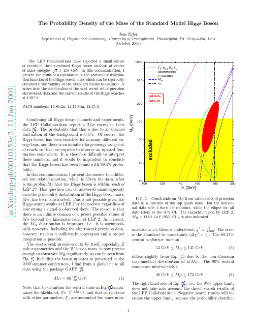
a r X i v :h e p -p h /0010153v 2 11 J a n 2001The Probability Density of the Mass of the Standard Model Higgs BosonJens ErlerDepartment of Physics and Astronomy,University of Pennsylvania,Philadelphia,PA 19104-6396,USA(October 2000)The LEP Collaborations have reported a small excess of events in their combined Higgs boson analysis at center of mass energies√tion function is eﬀectively being renormalized.For ex-ample,in a previous analysis[3]we found that the Higgs exclusion curve presented by the LEP Collaborations in-creased the95%upper limit by30GeV.The use of the Higgs exclusion curve,however,is only appropriate if no indication of an excess is observed.In general,it is more appropriate to consider the likelihood ratio for the data,Q LEP2=L(data|signal+background)p(data),(6)which must be satisﬁed once the likelihood,p(data|M H),and prior distribution,p(M H),are speciﬁed.p(data)≡ p(data|MH)p(M H)dM H in the denominator provides the proper normalization of the posterior distribution on the left hand side.Depending on the case at hand,the prior can1.contain additional information not included in thelikelihood model,2.contain likelihood functions obtained from previousmeasurements,3.or be chosen non-informative.Of course,the posterior does not depend on how infor-mation is separated into the likelihood and the prior.As for the present case,I choose the informative prior,p(M H)=Q LEP2p non−inf(M H),(7) where the non-informative part of the prior will be chosen asp non−inf(M H)=M−1H .(8)This choice corresponds to aﬂat prior in the variableln M H,and there are various ways to justify it[7].Onerationale is that aﬂat distribution is most natural for avariable deﬁned over all the real numbers.This is thecase for ln M H but not M2H.Also,it seems that a prioriit is equally likely that M H lies,say,between30and40GeV,or between300and400GeV.In any case,thesensitivity of the posterior to the(non-informative)priordiminishes rapidly with the inclusion of more data.Asdiscussed before,p(M H)is an improper prior but thelikelihood constructed from the precision measurementswill provide a proper posterior.Occasionally,the Bayesian method is criticized for theneed of a prior,which would introduce unnecessary sub-jectivity into the analysis.Indeed,care and good judge-ment is needed,but the same is true for the likelihoodmodel,which has to be speciﬁed in any statistical model.Moreover,it is appreciated among Bayesian practition-ers,that the explicit presence of the prior can be advan-tageous:it manifests model assumptions and allows forsensitivity checks.From the theorem(6)it is also clearthat any other method must correspond,mathematically,to speciﬁc choices for the prior.Thus,Bayesian methodsare more general and diﬀer rather in attitude:by theirstrong emphasis on the entire posterior distribution andby theirﬁrst principles setup.Including Q LEP2in this way,one obtains the95%CL upper limit M H≤201GeV,i.e.notwithstandingthe observed excess events,the information provided bythe Higgs searches at LEP2increase the upper limit by28GeV.Given extra parameters,ξi,the distribution func-tion of M H is deﬁned as the marginal distribution,p(M H|data)= p(M H,ξi|data) i p(ξi)dξi.If the like-lihood factorizes,p(M H,ξi)=p(M H)p(ξi),theξi depen-dence can be ignored.If not,but p(ξi|M H)is(approxi-mately)multivariate normal,thenχ2(M H,ξi)=χ2min(M H)+1∂ξi∂ξj(ξi−ξi min(M H))(ξj−ξj min(M H)).The latter applies to our case,whereξi=(m t,αs,α(M Z)).Integration yields,p(M H|data)∼√∂ξi∂ξj)−1,introducesa correction factor with a mild M H dependence.It cor-responds to a shift relative to the standard likelihoodmodel,χ2(M H)=χ2min(M H)+∆χ2(M H),where∆χ2(M H)≡lndet E(M H)FIG.2.Probability distribution function for the Higgs boson mass.The probability is shown for bin sizes of1GeV. Included are all available direct and indirect data.The shaded and unshaded regions each mark50%probability.I also include theory uncertainties from uncalculated higher orders.This increases the upper limit by5GeV, M H≤205GeV(95%CL).(11) The entire probability distribution is shown in Fig.2. Taking the data at face value,there is(as expected) a signiﬁcant peak around M H=115GeV,but more than half of the probability is for Higgs boson masses above the kinematic reach of LEP2(the median is at M H=119GeV).However,if one would double the in-tegrated luminosity and assume that the results would be similar to the present ones,one wouldﬁnd most of the probability concentrated around the peak.A similar statement will apply to Run II of the Tevatron at a time when about3to5fb−1of data have been collected. The described method is robust within the SM,but it should be cautioned that M H extracted from the preci-sion data is strongly correlated with certain new physics parameters.Likewise,the Higgs searches at LEP2de-pend on the predictions of signal and background expec-tations which are strictly calculable only within a spec-iﬁed theory.This note focussed on the Standard Model Higgs boson.Acknowledgements:This work was supported in part by the US Depart-ment of Energy grant EY–76–02–3071.。

Investigation of Color Aliasing of High Spatial Frequencies and Edges for Bayer-Pattern Sen

Investigation of Color Aliasing of High Spatial Frequencies and Edges for Bayer-Pattern Sensors and Foveon X3® Direct Image SensorsRudolph J. GuttoschFoveon, Inc.Santa Clara, CAAbstractThe reproduction of an edge and a high frequency bar pattern is examined for image sensors employing two different color sampling technologies: Bayer RGB color filter array, and Foveon X3 solid state full color. Simulations correlate well with actual images captured using sensors representing both technologies. Color aliasing artifacts in the Bayer mosaic case depend on whether an anti-aliasing optical lowpass filter is used, and are severe without such a filter. For both the edge image and the bar pattern, the Foveon X3 direct image sensor generates few or no color aliasing artifacts associated with sampling.1. Introduction1.1 Bayer BackgroundColor image data files typically viewed on computer monitors are made up of three complete planes of red, green, and blue data. Digital capture of an image with three complete planes was often accomplished with an image capture system consisting of a color separating prism and three image sensors affixed to the exit windows of the prism. Such devices produce high quality results, but require great precision in manufacturing and are costly, requiring image sensors and a prism to construct.The recent explosion of digital image capture devices in both the DSC (Digital Still Camera) and the cell phone markets has been fueled by the use of a less expensive alternative for color image capture. This alternative is known as the Bayer1 CFA (Color Filter Array), named after its inventor, Dr. Bryce Bayer, of the Eastman Kodak Company.The Bayer CFA is made up of a repeating array of red, green, and blue filter material deposited on top of each pixel in an array (Figure 1). These tiny filters enable what is normally a black-and-white sensor to create color images.Figure 1: Typical Bayer CFA showing the alternate sampling of red, green, and blue pixels.By using two green-filtered pixels for every red and blue, the Bayer CFA is designed to maximize the perceived sharpness in the luminance channel, which is composed mostly of green information. However, since the image plane is under-sampled by 50% to begin with, the full detail available in the optical image is not attained in the luminance sampled data. In addition, chrominance detail is lost due to the even lower sampling density of 25% in the red and blue channels in the sensor. Figure 2 shows a Bayer filter pattern decomposed into its constituent color components, showing the sparseness of the sampling. In order to create the required completely-populated image plane (i.e. three complete planes of red, green, and blue information), the Bayer CFA data must be interpolated, the process which fills in the voids shown in Figure 2.Figure 2: Decomposition of a typical Bayer CFA pattern into its components. Under-sampling in theimage plane results in lower sharpness than could otherwise be achieved. Further, gaps in the imageplane lead to color moiré artifacts.Introduced in the 1970’s, the Bayer CFA improved the state-of-the-art of image color image capture and reduced image capture cost. However, when considering the image quality vectors of sharpness and artifact control, the Bayer CFA represents an inefficient use of silicon area and imposes constraints on the digital camera designer. Due to the sparse nature of the sampling, the Bayer CFA imposes the need for the following:1.interpolation of the missing color data to create three complete color image planes (R, G, &B)2.sharpening of the image to account for the inherent reduction in the sharpness of theluminance and chrominance3.suppression of color aliasing artifacts resulting from incomplete sampling in the image planeand the phase offsets of the color channelsTo combat the third effect noted above, an optical blur filter, also known as an Anti-Aliasing filter, or an optical low-pass filter, (OLPF), is usually employed in consumer and professional digital cameras. Blur filters reduce the color aliasing artifacts caused by spatial phase differences among the color channels (i.e. the red, green, and blue filters are placed next to each other). Two blur filters are typically placed in the optical path: one to blur in the horizontal direction, the other in the vertical. The blur filters reduce color aliasing at the expense of image sharpness. In order to control costs, blur filters have not typically been used in digital cameras designed for cell phones. The effect of leaving out this component can be readily seen in images.1.2 Foveon X3 TechnologyAn alternative method for obtaining color images from a single chip monolithic imaging array is now available:2,3 the Foveon X3 direct image sensor. A direct image sensor is an image sensor that directly captures red, green, and blue light at each point in an image during a single exposure. Foveon X3 sensors take advantage of the natural light absorbing characteristics of silicon. Light of different wavelengths penetrating the silicon is absorbed at different depths -- high energy (blue) photons are absorbed near the surface, medium energy (green) photons in the middle, and low energy (red) photons are absorbed deeper in the material.4 In contrast to the lateral color sensing method in the Bayer CFA, X3 image sensors enable red, green, and blue pixels to be stacked vertically. A schematic representation of this vertical arrangement is shown in Figure 3.Figure 3: Schematic depiction of a Foveon X3 image sensor showing stacks of pixels, which recordcolor channels depth-wise in silicon.Figure 4 shows the color planes that result directly from image capture, without interpolation.Figure 4: Fully populated image sampling found in film scanners, color-separation prism cameras, andalso in Foveon X3 image sensors.Vertical stacking increases pixel density, thereby increasing the sharpness per unit area captured in the image plane. The stacks of red, green and blue pixels also eliminate the phase differences among the samples in color planes, thus eliminating false color patterns without additional processing. Blur filters are not necessary to combat color moiré patterns and the sharpness improvement for X3 image sensors in both luminance and chrominance can be measured using industry-standard techniques.52. MethodA Bayer CFA image sensor and a Foveon X3 image sensor were each simulated using a simplified model. The two sensors were exposed to two different stimuli in the simulation: an edge and a high frequency bar target. In order to achieve a processed image from Bayer CFA data, it is first necessary to interpolate, or fill in, the missing pixel data, a step not required for Foveon X3 image sensors. For this study, color interpolation was performed on the Bayer CFA using the bi-linear method shown in Figure 5 to create three complete planes of R, G,B data.R 1,2R R 2,2R 3,2R 4,1R 4,2R 1,4R 2,3R 2,4R 3,4R 4,3R 4,4B B B B 3,1B B 4,1B B B 2,3B B B 4,3R 11= R 11R 12= (R 11+ R 13)/2R 21= (R 11+ R 31)/2R 22= (R 11+ R 13+ R 31+ R 33)/4B 22= B 22B 23= (B 22+ B 24)/2B 32= (B 22+ B 42)/2B 33= (B 22+ B 24+ B 42+ B 44)/4G 22= (G 12+ G 32+ G 21+ G 23)/4G 23= G 23G 32= G 32G 33= (G 23+ G 43+ G 32+ G 34)/4Figure 5: Bayer CFA color sample positions and the color interpolation equations used in thisinvestigationOther, more complex algorithms are often used 6, and sometimes licensed 7. With the more complex algorithms, the overall performance of the color interpolation process can be improved; however, this comes with a significant penalty in both computation time and image processing device costs. In addition, no amount of added processing complexity can eliminate the fundamental samplingdisadvantages of a Bayer CFA. The simple color interpolation algorithm used in this analysis is widely applied in low-cost digital image capture systems where blur filters are also prohibitively expensive.An outline of the color interpolation steps used in the simulated images is illustrated in Figure 6. As the diagram shows, going from capture to finished image requires an extra color interpolation step for Bayer image sensors.Figure 6: Comparison of color image capture planes and resulting images for a simulated edge.1. Edge image projected onto image sensor.2. R, G, and B planes immediately after capture. Missing data for the Bayer case is evident.3. Bayer image planes after color interpolation, a step not required for Foveon X3 sensors.4. Resulting edge images.Bayer CFA Foveon X3Graphical representations of the edge applied to Bayer CFA and Foveon X3 image sensors are shown in figure 7; graphical representations of the high-frequency bar pattern case are given in Figure 8.Figure 7: Bayer CFA image sensor, left, and Foveon X3 image sensor, right, with simulated edgesuperimposed. Percentages refer to percent response, based on percent of area exposed, equivalent to a100% fill-factor pixel. Response normalized so that black = 0% and white = 100%. These percentageswere scaled to 8 bits for simulated image output.Image output was created and analyzed to show how each system reproduces the stimuli of interest. Optical effects and lens aberrations were specifically excluded from this analysis in order to gain a clear understanding of the contribution of the sensor sampling method on the output image quality. The aliasing response of the Bayer CFA was also investigated visually from a simulated bar pattern with a spatial frequency of 1/3 cycle per pixel location. This frequency is below the Nyquist rate of 1/2 cycle per pixel location. Although the bar pattern used in this analysis is synthesized, such patterns are commonly found in fabrics, vertical blinds, buildings, and are used in most standard imaging system resolution tests. An example of the graphical superposition of a high-frequency bar pattern on a Bayer CFA sensor and a Foveon X3 sensor is given in Figure 8.Figure 8: Bar pattern with frequency of 1/3 cycle/pixel location (top). Same bar pattern superimposed on Bayer CFA, left, and Foveon X3 sensors, right, with resulting relative responses (in percent).In order to compare the results of the image simulations with those obtained by commercially available image sensors, real-world images of an edge and a high-frequency bar target were captured using the cameras listed in the table below:Table 1: Cameras and sensors used to capture real-world images3. ResultsThe simulated edge target results are shown in Figure 9, and bar target results are shown in Figure 11. In order to validate the model and results of this study, real images of a slanted edge and bar pattern target were captured using both a Bayer CFA sensor and a Foveon X3 sensor. Those results are shown in Figures 10 and 13. Visual comparisons of the results clearly show that the model predicts the performance of real camera systems very accurately. Figure 12 shows a section of an IT-10 resolution chart captured with cameras and sensors from Table 1.Figure 9: Simulated Bayer CFA (left) and Foveon X3 image sensor (right) responses to slanted edge.Note lack of colored artifacts and sharper edge in the X3 sensor example.Figure 10: Real-world images obtained from cameras using, the Bayer CFA on a CCD image sensor,(left) and the Foveon X3 image sensor (right).Bayer CFA Camera Foveon X3 Camera Camera Roper Scientific Coolsnap Foveon F19 Reference Design Kit Image SensorSony ICX 2051392 x 1040 x 1Foveon F19 X3 Sensor1440 x 1088 x 3Pixel Size 4.65 µm 5.00 µmLens Pentax Cosmicar C-Mount Pentax Cosmicar C-MountFigure 11: Simulated result of imaging a high frequency bar pattern on a Bayer CFA (left) and a FoveonX3 sensor (right).Figure 12: Section of an IT10 resolution chart captured with Bayer CFA (left) and Foveon X3 (right)image sensors. Note the various color artifact patterns in the Bayer CFA case that depend on the inputfrequency. The numbers in the chart refer to the spatial frequency (multiply x100 to obtain Line Widthsper Picture Height, LW/PH). The region of interest for 1/3 cycle/pixel location (~700 LW/PH for both sensors) is shown in the red boxes. Detail from portions of these regions is shown in Figure 13.Figure 13: Digital camera output of a high frequency bar target (1/3 cycle/pixel location) for a Bayerimage sensor (left) and a Foveon X3 image sensor (right).4. DiscussionBoth the simulated and actual edge response for the Bayer CFA clearly show both sharpness reduction in the edge and false-color artifacts. Complete color sampling of the image plane, as demonstrated by the Foveon X3 direct image sensor, can eliminate the source of the image artifacts. The results can be obtained using a Foveon X3 sensor without the need for optical blur filters which would reduce image sharpness and add cost to the image capture system.In Figure 12, a comparison of the reproduction of an IT10 resolution chart is shown. In the Bayer case, interesting false color Moiré patterns crop up that are a function of the input frequency. For the Foveon X3 sensor, some luminance (i.e. not false color) Moiré, which is typical of sampled data systems, is visible.The bar pattern results show that even at frequencies lower than Nyquist, the Bayer CFA imager will add color artifacts to black-and-white subjects. Using a bar pattern, it is quite simple to produce color artifacts both in simulations and in actual use. Again, by completely sampling the image plane, the Foveon X3 sensor provides a black-and-white reproduction of a black-and-white subject.5. ConclusionThe performance of traditional Bayer CFA image sensor technology was compared to Foveon X3 image sensor technology using both a simple simulation and real-world image capture. The results of both the simulation and the test images clearly show the advantages of Foveon technology with respect to color artifacts and sharpness. A Bayer CFA image sensor without a blur filter shows significant color artifacts resulting from the improper sampling. While the combination of a blur filter and increased color interpolation complexity can be used to partially compensate for the deficiencies in the Bayer sensor, the underlying problem is inherent and comes from undersampling in the image plane. The costs of the attempts at working around the problems with Bayer CFA technology are direct: added component costs due to blur filter, a more advanced image processor device as well as additional compute time. In applications where cost, power, and size are critical, decreasing performance in these key areas is not an acceptable tradeoff to make in order to ensure good image quality.By fully sampling color in the image plane, Foveon X3 direct image sensors avoid the color artifacts and provide increased sharpness without adding cost to the digital camera system.References1 B. E. Bayer, “Color Imaging Array,” US Patent 3,971,065, 1976.2 R. B. Merrill, “Color Separation in an Active Pixel Cell Imaging Array Using a Triple-Well-Structure,” US Patent 5,965,875, 1999.3 R. F. Lyon and P. M. Hubel, “Eyeing the Camera: into the Next Century”, Tenth Color Imaging Conference: Color Science and Engineering Systems, Technologies, Applications; Scottsdale, Arizona; November, 2002.4 A. J. P. Theuwissen, Solid-State Imaging with Charged-Coupled Devices, Kluwer Academic Press, Dordrecht, 1995.5 P. M. Hubel, J. Liu, and R. J. Guttosch, Spatial Frequency Response of Color Image Sensors: Bayer Color Filters and Foveon X3; Proc. SPIE Vol. 5301, p. 402-407, 2004.6 R. Ramanath, et. al, “Demosaicking Methods for Bayer color arrays”, Journal of Electronic Imaging, July 2002 pp. 306-315.7 J. F. Hamilton and J. E. Adams, “Adaptive color plane interpolation in single sensor color electronic camera,” US Patent No. 5, 629, 734 (1997).© 1998-2005 Foveon, Inc. Foveon, X3, and the X3 logo are registered trademarks of Foveon, Inc.。

周云朋

2、COSMO-SAC模型选择离子液体萃取剂的步骤
对于基于COSMO的模型而言，最耗时的计算是量子化学计算，且计算时间随着分子中原子个数的增加呈几何级数增长。因此,为了减少计算工作量，离子液体分成阳离子和阴离子分别进行量子化学计算，获得各自的σ-图谱，然后将阳离子和阴离子的 σ-图谱加和得到离子液体的σ-图谱。
2、COSMO-SAC模型选择离子液体萃取剂的步骤
b、萃取剂的模糊综合评判评判因素集Ｕ＝｛β，ｍ，SL｝＝｛ｕ１，ｕ２，ｕ３｝。对Ｕ中所用的因素均设评语集Ｖ=｛优｝。
萃取剂的模糊综合评判公式为：Ｂ=AR=［ｂ１，ｂ２…ｂｋ］。其中，Ａ为权重分配集，Ｒ为模糊转换矩阵。式中ｒｉｊ是第ｊ个被评判对象中第ｉ个元素对Ｖ的隶属度，隶属度函数如下
谢谢大家！
2、COSMO-SAC模型选择离子液体萃取剂的步骤
rA 其中， , B 为组分Ａ在组分Ｂ中的无限稀释活度因 r 子； A, S 为组分Ａ在萃取剂Ｓ中的无限稀释活度因子； rB , S 为组分Ｂ在萃取剂Ｓ中的无限稀释活度因子；为萃取剂Ｓ在组分Ｂ中的无限稀释活度因子。 rS ,B
2、COSMO-SAC模型选择离子液体萃取剂的步骤
（6）、判断迭代次数Ｎ是否大于最大迭代次数Ｎmax，如果Ｎ≤Ｎmax，转入步骤（2）；（7）、将满足要求的萃取剂按照模糊综合评判排序，输出结果。
二、后期工作计划
1、继续加深对materials studio(MS)出适合分离其体系的离子液体。
2、COSMO-SAC模型选择离子液体萃取剂的步骤
其中，α′是错位能常数，通过标准片段表面积aeff计算，如上式所示。chb是氢键作用常数，σhb是氢键作用截断值，σacc和σdon分别是σｍ和σｎ的最大值和最小。 b、计算活度因子的组合项。计算公式如下：

yantubbs-The hardening soil model, Formulation and verification

The hardening soil model: Formulation and verificationT. SchanzLaboratory of Soil Mechanics, Bauhaus-University Weimar, GermanyP.A. VermeerInstitute of Geotechnical Engineering, University Stuttgart, GermanyP.G. BonnierP LAXIS B.V., NetherlandsKeywords: constitutive modeling, HS-model, calibration, verificationABSTRACT: A new constitutive model is introduced which is formulated in the framework of classical theory of plasticity. In the model the total strains are calculated using a stress-dependent stiffness, different for both virgin loading and un-/reloading. The plastic strains are calculated by introducing a multi-surface yield criterion. Hardening is assumed to be isotropic depending on both the plastic shear and volumetric strain. For the frictional hardening a non-associated and for the cap hardening an associated flow rule is assumed.First the model is written in its rate form. Therefor the essential equations for the stiffness mod-ules, the yield-, failure- and plastic potential surfaces are given.In the next part some remarks are given on the models incremental implementation in the P LAXIS computer code. The parameters used in the model are summarized, their physical interpre-tation and determination are explained in detail.The model is calibrated for a loose sand for which a lot of experimental data is available. With the so calibrated model undrained shear tests and pressuremeter tests are back-calculated.The paper ends with some remarks on the limitations of the model and an outlook on further de-velopments.1INTRODUCTIONDue to the considerable expense of soil testing, good quality input data for stress-strain relation-ships tend to be very limited. In many cases of daily geotechnical engineering one has good data on strength parameters but little or no data on stiffness parameters. In such a situation, it is no help to employ complex stress-strain models for calculating geotechnical boundary value problems. In-stead of using Hooke's single-stiffness model with linear elasticity in combination with an ideal plasticity according to Mohr-Coulomb a new constitutive formulation using a double-stiffness model for elasticity in combination with isotropic strain hardening is presented.Summarizing the existing double-stiffness models the most dominant type of model is the Cam-Clay model (Hashiguchi 1985, Hashiguchi 1993). To describe the non-linear stress-strain behav-iour of soils, beside the Cam-Clay model the pseudo-elastic (hypo-elastic) type of model has been developed. There an Hookean relationship is assumed between increments of stress and strain and non-linearity is achieved by means of varying Young's modulus. By far the best known model of this category ist the Duncan-Chang model, also known as the hyperbolic model (Duncan & Chang 1970). This model captures soil behaviour in a very tractable manner on the basis of only two stiff-ness parameters and is very much appreciated among consulting geotechnical engineers. The major inconsistency of this type of model which is the reason why it is not accepted by scientists is that, in contrast to the elasto-plastic type of model, a purely hypo-elastic model cannot consistently dis-tinguish between loading and unloading. In addition, the model is not suitable for collapse load computations in the fully plastic range.12These restrictions will be overcome by formulating a model in an elasto-plastic framework in this paper. Doing so the Hardening-Soil model, however, supersedes the Duncan-Chang model by far. Firstly by using the theory of plasticity rather than the theory of elasticity. Secondly by includ-ing soil dilatancy and thirdly by introducing a yield cap.In contrast to an elastic perfectly-plastic model, the yield surface of the Hardening Soil model is not fixed in principal stress space, but it can expand due to plastic straining. Distinction is made between two main types of hardening, namely shear hardening and compression hardening. Shear hardening is used to model irreversible strains due to primary deviatoric loading. Compression hardening is used to model irreversible plastic strains due to primary compression in oedometer loading and isotropic loading.For the sake of convenience, restriction is made in the following sections to triaxial loading conditions with 2σ′ = 3σ′ and 1σ′ being the effective major compressive stress.2 CONSTITUTIVE EQUATIONS FOR STANDARD DRAINED TRIAXIAL TESTA basic idea for the formulation of the Hardening-Soil model is the hyperbolic relationship be-tween the vertical strain ε1, and the deviatoric stress, q , in primary triaxial loading. When subjected to primary deviatoric loading, soil shows a decreasing stiffness and simultaneously irreversible plastic strains develop. In the special case of a drained triaxial test, the observed relationship be-tween the axial strain and the deviatoric stress can be well approximated by a hyperbola (Kondner& Zelasko 1963). Standard drained triaxial tests tend to yield curves that can be described by:The ultimate deviatoric stress, q f , and the quantity q a in Eq. 1 are defined as:The above relationship for q f is derived from the Mohr-Coulomb failure criterion, which involves the strength parameters c and ϕp . As soon as q = q f , the failure criterion is satisfied and perfectly plastic yielding occurs. The ratio between q f and q a is given by the failure ratio R f , which should obviously be smaller than 1. R f = 0.9 often is a suitable default setting. This hyperbolic relationship is plotted in Fig. 1.2.1 Stiffness for primary loadingThe stress strain behaviour for primary loading is highly nonlinear. The parameter E 50 is the con-fining stress dependent stiffness modulus for primary loading. E 50is used instead of the initial modulus E i for small strain which, as a tangent modulus, is more difficult to determine experimen-tally. It is given by the equation:ref E 50is a reference stiffness modulus corresponding to the reference stress ref p . The actual stiff-ness depends on the minor principal stress, 3σ′, which is the effective confining pressure in a tri-axial test. The amount of stress dependency is given by the power m . In order to simulate a loga-rithmic stress dependency, as observed for soft clays, the power should be taken equal to 1.0. As a3Figure 1. Hyperbolic stress-strain relation in primary loading for a standard drained triaxial test.secant modulus ref E 50 is determined from a triaxial stress-strain-curve for a mobilization of 50% ofthe maximum shear strength q f .2.2 Stiffness for un-/reloadingFor unloading and reloading stress paths, another stress-dependent stiffness modulus is used:where ref urE is the reference Young's modulus for unloading and reloading, corresponding to the reference pressure σ ref . Doing so the un-/reloading path is modeled as purely (non-linear) elastic.The elastic components of strain εe are calculated according to a Hookean type of elastic relation using Eqs. 4 + 5 and a constant value for the un-/reloading Poisson's ratio υur .For drained triaxial test stress paths with σ2 = σ3 = constant, the elastic Young's modulus E ur re-mains constant and the elastic strains are given by the equations:Here it should be realised that restriction is made to strains that develop during deviatoric loading,whilst the strains that develop during the very first stage of the test are not considered. For the first stage of isotropic compression (with consolidation), the Hardening-Soil model predicts fully elastic volume changes according to Hooke's law, but these strains are not included in Eq. 6.2.3 Yield surface, failure condition, hardening lawFor the triaxial case the two yield functions f 12 and f 13 are defined according to Eqs. 7 and 8. Here4Figure 2. Successive yield loci for various values of the hardening parameter γ p and failure surface.the measure of the plastic shear strain γ p according to Eq. 9 is used as the relevant parameter forthe frictional hardening:with the definitionIn reality, plastic volumetric strains p υε will never be precisely equal to zero, but for hard soils plastic volume changes tend to be small when compared with the axial strain, so that the approxi-mation in Eq. 9 will generally be accurate.For a given constant value of the hardening parameter, γ p , the yield condition f 12 = f 13 = 0 can be visualised in p'-q-plane by means of a yield locus. When plotting such yield loci, one has to use Eqs. 7 and 8 as well as Eqs. 3 and 4 for E 50 and E ur respectively. Because of the latter expressions,the shape of the yield loci depends on the exponent m . For m = 1.0 straight lines are obtained, but slightly curved yield loci correspond to lower values of the exponent. Fig. 2 shows the shape of successive yield loci for m = 0.5, being typical for hard soils. For increasing loading the failure sur-faces approach the linear failure condition according to Eq. 2.2.4 Flow rule, plastic potential functionsHaving presented a relationship for the plastic shear strain, γ p , attention is now focused on the plastic volumetric strain p υε. As for all plasticity models, the Hardening-Soil model involves a re-lationship between rates of plastic strain, i.e. a relationship between p υε and p γ . This flow rule hasthe linear form:5Clearly, further detail is needed by specifying the mobilized dilatancy angle m ψ. For the presentmodel, the expression:is adopted, where cv ϕ is the critical state friction angle, being a material constant independent ofdensity (Schanz & Vermeer 1996), and m ϕ is the mobilized friction angle:The above equations correspond to the well-known stress-dilatancy theory (Rowe 1962, Rowe 1971), as explained by (Schanz & Vermeer 1996). The essential property of the stress-dilatancy theory is that the material contracts for small stress ratios m ϕ < cv ϕ, whilst dilatancy occurs for high stress ratios m ϕ < cv ϕ. At failure, when the mobilized friction angle equals the failure angle,p ϕ, it is found from Eq. 11 that:Hence, the critical state angle can be computed from the failure angles p ϕand p ψ. The above defi-nition of the flow rule is equivalent to the definition of definition of the plastic potential functionsg 12 and g 13 according to:Using theKoiter-rule (Koiter 1960) for yielding depending on two yield surfaces (Multi-surface plasticity ) one finds:Calculating the different plastic strain rates by this equation, Eq. 10 directly follows.3 TIME INTEGRATIONThe model as described above has been implemented in the finite element code P LAXIS (Vermeer& Brinkgreve 1998). To do so, the model equations have to be written in incremental form. Due to this incremental formulation several assumptions and modifications have to be made, which will be explained in this section.During the global iteration process, the displacement increment follows from subsequent solu-tion of the global system of equations:where K is the global stiffness matrix in which we use the elastic Hooke's matrix D , f ext is a global load vector following from the external loads and f int is the global reaction vector following from the stresses. The stress at the end of an increment σ 1 can be calculated (for a given strain increment ∆ε) as:6whereσ0 , stress at the start of the increment,∆σ , resulting stress increment,4D , Hooke's elasticity matrix, based on the unloading-reloading stiffness,∆ε , strain increment (= B ∆u ),γ p , measure of the plastic shear strain, used as hardening parameter,∆Λ , increment of the non-negative multiplier,g , plastic potential function.The multiplier Λ has to be determined from the condition that the function f (σ1, γ p ) = 0 has to be zero for the new stress and deformation state.As during the increment of strain the stresses change, the stress dependant variables, like the elasticity matrix and the plastic potential function g , also change. The change in the stiffness during the increment is not very important as in many cases the deformations are dominated by plasticity.This is also the reason why a Hooke's matrix is used. We use the stiffness matrix 4D based on the stresses at the beginning of the step (Euler explicit ). In cases where the stress increment follows from elasticity alone, such as in unloading or reloading, we iterate on the average stiffness during the increment.The plastic potential function g also depends on the stresses and the mobilized dilation angle m ψ. The dilation angle for these derivatives is taken at the beginning of the step. The implementa-tion uses an implicit scheme for the derivatives of the plastic potential function g . The derivatives are taken at a predictor stress σtr , following from elasticity and the plastic deformation in the previ-ous iteration:The calculation of the stress increment can be performed in principal stress space. Therefore ini-tially the principal stresses and principal directions have to be calculated from the Cartesian stresses, based on the elastic prediction. To indicate this we use the subscripts 1, 2 and 3 and have 321σσσ≥≥ where compression is assumed to be positive.Principal plastic strain increments are now calculated and finally the Cartesian stresses have to be back-calculated from the resulting principal constitutive stresses. The calculation of the consti-tutive stresses can be written as:From this the deviatoric stress q (σ1 – σ3) and the asymptotic deviatoric stress q a can be expressed in the elastic prediction stresses and the multiplier ∆Λ:7whereFor these stresses the functionshould be zero. As the increment of the plastic shear strain ∆γ p also depends linearly on the multi-plier ∆Λ, the above formulae result in a (complicated) quadratic equation for the multiplier ∆Λwhich can be solved easily. Using the resulting value of ∆Λ, one can calculate (incremental)stresses and the (increment of the) plastic shear strain.In the above formulation it is assumed that there is a single yield function. In case of triaxial compression or triaxial extension states of stress there are two yield functions and two plastic po-tential functions. Following (Koiter 1960) one can write:where the subscripts indicate the principal stresses used for the yield and potential functions. At most two of the multipliers are positive. In case of triaxial compression we have σ2 = σ3, Λ23 = 0and we use two consistency conditions instead of one as above. The increment of the plastic shear strain has to be expressed in the multipliers. This again results in a quadratic equation in one of the multipliers.When the stresses are calculated one still has to check if the stress state violates the yield crite-rion q ≤ q f . When this happens the stresses have to be returned to the Mohr-Coulomb yield surface.4 ON THE CAP YIELD SURFACEShear yield surfaces as indicated in Fig. 2 do not explain the plastic volume strain that is measured in isotropic compression. A second type of yield surface must therefore be introduced to close the elastic region in the direction of the p-axis. Without such a cap type yield surface it would not be possible to formulate a model with independent input of both E 50 and E oed . The triaxial modulus largely controls the shear yield surface and the oedometer modulus controls the cap yield surface.In fact, ref E 50largely controls the magnitude of the plastic strains that are associated with the shear yield surface. Similarly, ref oedE is used to control the magnitude of plastic strains that originate from the yield cap. In this section the yield cap will be described in full detail. To this end we consider the definition of the cap yield surface (a = c cot ϕ):8where M is an auxiliary model parameter that relates to NC K 0 as will be discussed later. Further more we have p = (σ1 + σ2+ σ3) andwithq is a special stress measure for deviatoric stresses. In the special case of triaxial compression it yields q = (σ1 – σ3) and for triaxial extension reduces to q = α (σ1 –σ3). For yielding on the cap surface we use an associated flow rule with the definition of the plastic potential g c :The magnitude of the yield cap is determined by the isotropic pre-consolidation stress p c . For the case of isotropic compression the evolution ofp c can be related to the plastic volumetric strain rate p v ε:Here H is the hardening modulus according to Eq. 32, which expresses the relation between theelastic swelling modulus K s and the elasto-plastic compression modulus K c for isotropic compres-sion:From this definition follows a stress dependency of H . For the case of isotropic compression we haveq = 0 and therefor c p p=. For this reason we find Eq. 33 directly from Eq. 31:The plastic multiplier c Λ referring to the cap is determined according to Eq. 35 using the addi-tional consistency condition:Using Eqs. 33 and 35 we find the hardening law relating p c to the volumetric cap strain c v ε:9Figure 3. Representation of total yield contour of the Hardening-Soil model in principal stress space for co-hesionless soil.The volumetric cap strain is the plastic volumetric strain in isotropic compression. In addition to the well known constants m and σref there is another model constant H . Both H and M are cap pa-rameters, but they are not used as direct input parameters. Instead, we have relationships of theform NC K 0=NC K 0(..., M, H ) and ref oed E = ref oed E (..., M, H ), such that NC K 0and ref oed E can be used as in-put parameters that determine the magnitude of M and H respectively. The shape of the yield cap is an ellipse in p – q ~-plane. This ellipse has length p c + a on the p -axis and M (p c+ a ) on the q ~-axis.Hence, p c determines its magnitude and M its aspect ratio. High values of M lead to steep caps un-derneath the Mohr-Coulomb line, whereas small M -values define caps that are much more pointed around the p -axis.For understanding the yield surfaces in full detail, one should consider Fig. 3 which depicts yield surfaces in principal stress space. Both the shear locus and the yield cap have the hexagonal shape of the classical Mohr-Coulomb failure criterion. In fact, the shear yield locus can expand up to the ultimate Mohr-Coulomb failure surface. The cap yield surface expands as a function of the pre-consolidation stress p c .5 PARAMETERS OF THE HARDENING-SOIL MODELSome parameters of the present hardening model coincide with those of the classical non-hardening Mohr-Coulomb model. These are the failure parameters ϕp ,, c and ψp . Additionally we use the ba-sic parameters for the soil stiffness:ref E 50, secant stiffness in standard drained triaxial test,ref oedE , tangent stiffness for primary oedometer loading and m , power for stress-level dependency of stiffness.This set of parameters is completed by the following advanced parameters:ref urE , unloading/ reloading stiffness,10v ur , Poisson's ratio for unloading-reloading,p ref , reference stress for stiffnesses,NC K 0, K 0-value for normal consolidation andR f , failure ratio q f / q a .Experimental data on m , E 50 and E oed for granular soils is given in (Schanz & Vermeer 1998).5.1 Basic parameters for stiffnessThe advantage of the Hardening-Soil model over the Mohr-Coulomb model is not only the use of a hyperbolic stress-strain curve instead of a bi-linear curve, but also the control of stress level de-pendency. For real soils the different modules of stiffness depends on the stress level. With theHardening-Soil model a stiffness modulus ref E 50is defined for a reference minor principal stress of σ3 = σref . As some readers are familiar with the input of shear modules rather than the above stiff-ness modules, shear modules will now be discussed. Within Hooke's theory of elasticity conversion between E and G goes by the equation E = 2 (1 + v ) G . As E ur is a real elastic stiffness, one may thus write E ur = 2 (1 + v ur ) G ur , where G ur is an elastic shear modulus. In contrast to E ur , the secant modulus E 50 is not used within a concept of elasticity. As a consequence, there is no simple conver-sion from E 50 to G 50. In contrast to elasticity based models, the elasto-plastic Hardening-Soil model does not involve a fixed relationship between the (drained) triaxial stiffness E 50 and the oedometer stiffness E oed . Instead, these stiffnesses must be given independently. To define the oedometer stiff-ness we usewhere E oed is a tangent stiffness modulus for primary loading. Hence, ref oed E is a tangent stiffness ata vertical stress of σ1 = σref .5.2 Advanced parametersRealistic values of v ur are about 0.2. In contrast to the Mohr-Coulomb model, NC K 0 is not simply a function of Poisson's ratio, but a proper input parameter. As a default setting one can use the highly realistic correlation NC K 0= 1 – sin ϕp . However, one has the possibility to select different values.All possible different input values for NC K 0 cannot be accommodated for. Depending on other pa-rameters, such as E 50, E oed , E ur and v ur , there happens to be a lower bound on NC K 0. The reason for this situation will be explained in the next section.5.3 Dilatancy cut-offAfter extensive shearing, dilating materials arrive in a state of critical density where dilatancy has come to an end. This phenomenon of soil behaviour is included in the Hardening-Soil model by means of a dilatancy cut-off . In order to specify this behaviour, the initial void ratio, e 0, and the maximum void ratio, e cv , of the material are entered. As soon as the volume change results in a state of maximum void, the mobilized dilatancy angle, ψm , is automatically set back to zero, as in-dicated in Eq. 38 and Fig. 4:11Figure 4. Resulting strain curve for a standard drained triaxial test including dilatancy cut-off.The void ratio is related to the volumetric strain, εv by the relationship:where an increment of εv is negative for dilatancy. The initial void ratio, e 0, is the in-situ void ratio of the soil body. The maximum void ratio, e cv , is the void ratio of the material in a state of critical void (critical state).6 CALIBRATION OF THE MODELIn a first step the Hardening-Soil model was calibrated for a sand by back-calculating both triaxial compression and oedometer tests. Parameters for the loosely packed Hostun-sand (e 0 = 0.89), a well known granular soil in geotechnical research, are given in Tab. 1. Figs. 5 and 6 show the satis-fying comparison between the experimental (three different tests) and the numerical result. For the oedometer tests the numerical results consider the unloading loop at the maximum vertical load only.7 VERIFICATION OF THE MODEL7.1 Undrained behaviour of loose Hostun-sandIn order to verify the model in a first step two different triaxial compression tests on loose Hostun-sand under undrained conditions (Djedid 1986) were simulated using the identical parameter from the former calibration. The results of this comparison are displayed in Figs. 7 and 8.In Fig. 7 we can see that for two different confining pressures of σc = 300 and 600 kPa the stress paths in p-q-space coincide very well. For deviatoric loads of q ≈ 300 kPa excess porewater pres-sures tend to be overestimated by the calculations.Additionally in Fig. 8 the stress-strain-behaviour is compared in more detail. This diagram con-tains two different sets of curves. The first set (•, ♠) relates to the axial strain ε1 at the horizontal12Figure 5. Comparison between the numerical (•) and experimental results for the oedometer tests.Figure 6. Comparison between the numerical (•) and experimental results for the drained triaxial tests (σ3 = 300 kPa) on loose Hostun-sand.and the effective stress ratio 31/σσ′′ on the vertical (left) axis. The second set (o , a ) refers to the normalised excess pore water pressure ∆u /σc on the right vertical axis. Experimental results forboth confining stresses are marked by symbols, numerical results by straight and dotted lines.Analysing the amount of effective shear strength it can be seen that the maximum calculated stress ratio falls inside the range of values from the experiments. The variation of effective friction from both tests is from 33.8 to 35.4 degrees compared to an input value of 34 degrees. Axial stiff-ness for a range of vertical strain of ε1 < 0.05 seems to be slightly over-predicted by the model. Dif-ferences become more pronounced for the comparison of excess pore water pressure generation.Here the calculated maximum amount of ∆u is higher then the measured values. The rate of de-crease in ∆u for larger vertical strain falls in the range of the experimental data.Table 1. Parameters of loose Hostun-sand.v urm ϕp ψp ref ref s E E 50/ref ref ur E E 50/ref E 500.200.6534° 0° 0.8 3.0 20 MPa13Figure 7. Undrained behaviour of loose Hostun-sand: p-q-plane.Figure 8. Undrained behaviour of loose Hostun-sand: stress-strain relations.7.2 Pressuremeter test GrenobleThe second example to verify the Hardening-Soil model is a back-calculation of a pressuremeter test on loose Hostun-sand. This test is part of an experimental study using the calibration chamber at the IMG in Grenoble (Branque 1997). This experimental testing facility is shown in Fig. 9.The cylindrical calibration chamber has a height of 150 cm and a diameter of 120 cm. In the test considered in the following a vertical surcharge of 500 kPa is applied at the top of the soil mass by a membrane. Because of the radial deformation constraint the state of stress can be interpreted in this phase as under oedometer conditions. Inside the chamber a pressuremeter sonde of a radius r 0 of 2.75 cm and a length of 16 cm is placed. For the test considered in the following example there was loose Hostun-sand (D r ≈ 0.5) of a density according to the material parameters as shown in Tab. 1 placed around the pressuremeter by pluviation. After the installation of the device and the filling of the chamber the pressure is increased and the resulting volume change is registered.14Figure 9. Pressuremeter Grenoble .This experimental setup was modeled within a FE-simulation as shown in Fig. 10. On the left hand side the axis-symmetric mesh and its boundary conditions is displayed. The dimensions are those of the complete calibration chamber. In the left bottom corner of the geometry the mesh is finer because there the pressuremeter is modeled.In the first calculation phase the vertical surcharge load A is applied. At the same time the hori-zontal load B is increased the way practically no deformations occur at the free deformation bound-ary in the left bottom corner. In the second phase the load group A is kept constant and the load group B is increased according to the loading history in the experiment. The (horizontal) deforma-tions are analysed over the total height of the free boundary. In order to (partly) get rid of the de-formation constrains at the top of this boundary, marked point A in the detail on the right hand side of Fig. 10 two interfaces were placed crossing each other in point A . Fig. 11 shows the comparison of the experimental and numerical results for the test with a vertical surcharge of 500 kPa.On the vertical axis the pressure (relating to load group B ) is given and on the horizontal axis the volumetric deformation of the pressuremeter. Because the calculation was run taking into ac-count large deformations (updated mesh analysis ) the pressure p in the pressuremeter has to be cal-culated from load multiplier ΣLoad B according to Eq. 40, taking into account the mean radial de-formation ∆r of the free boundary:The agreement between the experimental and the numerical data is very good, both for the initial part of phase 2 and for larger deformations of up to 30%.。

A 3-D Quasi-Zero-Stiffness-Based Sensor System for Absolute Motion Measurement

A3-D Quasi-Zero-Stiffness-Based Sensor System for Absolute Motion Measurement and Application in Active Vibration ControlXiuting Sun,Xingjian Jing,Member,IEEE,Li Cheng,and Jian XuAbstract—A novel3-D quasi-zero-stiffness(3DQZS)system is proposed to construct a3-D sensor system for absolute motion measurement in vibration systems.The3DQZS system is achieved by employing a predeformed scissor-like structure.With mathe-matical modeling and the harmonic balance method,the nonlinear dynamic response of the3-D sensor system is deeply analyzed. It is shown that this novel3DQZS-based sensor system is very effective and reliable in3-D absolute motion measurement in vi-bration systems.A case study in active vibration control using the proposed3-D sensor indicates that much better vibration control performance can be readily achieved compared with conventional methods using a similar linear feedback controller.This novel sen-sor system should provide an alternative or much better solution to many vibration control problems in various engineering practices.Index Terms—Active vibration control,nonlinear system,quasi-zero stiffness(QZS),scissor-like structure(SLS),vibration sensor.I.I NTRODUCTIONI N V ARIOUS engineering practices for system identiﬁca-tion[1]–[3],control[4]–[12],[31]–[33],andﬁlter design [13],[14],system state measurement or estimation has always been a critical task because the control of vibration platforms (e.g.,vehicle suspension,instrument protection in ships or UA V, etc.)usually requires accurate knowledge of full system states with respect to a global coordinate system in active/semiactive control for better vibration suppression performance[9]–[12]. Therefore,various mechatronic systems are introduced as sen-sors for motion measurement[15]–[19].For measurement of ab-solute displacement or velocity,although some advanced mea-surement technology could be applied such as inertial sensors [15],radars or laser technology[16]–[19],etc.,realistic issues Manuscript received March7,2014;revised June20,2014;accepted June 25,2014.Date of publication August6,2014;date of current version October3, 2014.Recommended by Technical Editor M.Iwasaki.This work was supported in part by the National Natural Science Foundation of China(No.61374041), in part by the GRF projects of HK RGC(15206514,517810),and in part by the internal Research Grants of The Hong Kong Polytechnic University. (Corresponding author:Xingjian Jing).X.Sun is with the Department of Mechanical Engineering,The Hong Kong Polytechnic University,Hung Hom,Hong Kong,and also with the School of Aerospace Engineering and Applied Mechanics,Tongji University,Shanghai 200092,China(e-mail:05mech_sunxiuting@).X.Jing is with the Department of Mechanical Engineering,The Hong Kong Polytechnic University,Hung Hom,Hong Kong,and also with The Hong Kong Polytechnic University Shenzhen Research Institute,Shenzhen518057,China (e-mail:mmjxj@.hk;xingjian.jing@).L.Cheng is with the Department of Mechanical Engineering,The Hong Kong Polytechnic University,Hung Hom,Hong Kong.J.Xu is with School of Aerospace Engineering and Applied Mechanics, Tongji University,Shanghai200092,China.Digital Object Identiﬁer10.1109/TMECH.2014.2338932related to accuracy,installation and/or development cost would have to be considered.Accelerometers are often applied to mea-sure absolute acceleration in a vibrating system.But absolute motion of a system could not be accurately recovered from acceleration signals.Although some existing algorithms(e.g., linearﬁlters)could be used to estimate unmeasured states(e.g., displacement)from measured ones(e.g.,acceleration),it would induce problems to control systems such as time delay due to computation cost.It is known that time delay could easily dete-riorate the stability of a dynamic system and bring complexity for analysis and design[20]–[23].Even though for some cases [24]–[26]in vibration absorbers,time delay could beneﬁt vi-bration suppression when absolute displacement can be used in feedback control,the value of the time delay should be set in certain critical ranges with the help of precise instruments such as signal ampliﬁcation and readout devices.In order to conveniently and accurately measure absolute mo-tion for vibration control of vibration systems such as vehicle suspension systems or instrument protection in ships or UA V, etc.,a novel three-direction sensor(3DS)system is proposed in this study.The sensor is designed by employing a novel3-D quasi-zero-stiffness(3DQZS)vibration isolation system.The latter can achieve excellent passive nonlinear vibration isola-tion using a predeformed scissor-like structure,and this scissor-like structure was shown to be an excellent quasi-zero-stiffness (QZS)system recently in[27].Different from existing QZS vi-bration isolators in[28]–[30]effective only for one-direction (typically composed by two horizontal precompression springs and a vertical spring),the proposed3DQZS system is con-structed by two horizontal scissor-like structures(SLSs)with predeformation and vertical springs,which can realize QZS property in three directions.Because of this remarkable advan-tage of the3DQZS system,the relative motion between the 3DQZS system and the base structure can be sufﬁciently close to the absolute motion of the base structure.Moreover,the stiff-ness characteristics and geometric parameters of the3DQZS system can be easily designed and adjusted so as to greatly in-crease measurement accuracy in three directions.The proposed 3-D sensor is easy to design and implement in practice and some problems as mentioned above(e.g.,time delay,high cost)could be reasonably avoided.Besides theoretical analysis,a case study in active vibration control using this novel sensor vindicates the effectiveness.The rest of the paper is organized as follows.The structure of the novel3-D sensor system is introduced in Section II which is modeled through the Lagrange principle[34].Then,relative1083-4435©2014IEEE.Personal use is permitted,but republication/redistribution requires IEEE permission.See /publications standards/publications/rights/index.html for more information.Fig.1.Structural diagram of(a)the proposed absolute motion sensor and (b)its application to a vibration system.motion is compared to absolute motion of the vibration mass for different base excitations.A method for signal rectiﬁcation for accuracy improvement is discussed in Section IV.Section V shows an application of the novel sensor in feedback control.A conclusion is drawn thereafter.II.T HREE-D IMENSIONAL S ENSOR S YSTEM AND I TS M ODELING A.Structure of the Sensor SystemFig.1(a)is the proposed3-D sensor which can be used to measure absolute motion of a vibration system in three different directions.In the structure of the3-D sensor,M2is a small mass which includes the mass of two relative motion Sensors1and 2.The mass M2is connected to two n-layer SLSs with springs whose stiffness is k1and original length is l10.And two vertical springs whose stiffness is k2and original length is l20.Fig.1(b)shows the structural diagram of the3-D sensor used in a vibration platform with mass M1.The vibration platform is supposed to be connected to the base with horizontal springs whose linear stiffness is k xl and nonlinear stiffness k xn,verti-cal springs whose linear stiffness is k y l and nonlinear stiffness k y n,and two dampers with damping coefﬁcients c x and c y.All the structural parameters and their default values are listed in Table I in the Appendix.Without loss of specialty,the base ex-citations are supposed in horizontal direction z x(t)and vertical direction z y(t).The absolute vibration displacements of mass M1are denoted by x1(t)and y1(t),respectively.Similarly,the absolute vibration displacements of the mass M2are denoted by x2(t)and y2(t).Sensors1and2are the two relative mo-tion sensors whose signals obtained are the relative motions (displacement/velocity)between the mass M2and M1for two directions.The variables of the system in Fig.1are listed in Table II in the Appendix.B.Geometrical RelationsIn order to model this dynamic system to obtain relative and absolute motion,the geometrical relations and deformations of each spring and component in the system should be analyzed. Fig.2is the right-side SLS in the3-D sensor.Fig.2shows the deformation of the right-side SLS in the 3-D sensor.After deformation,the length of the spring inthe Fig.2.Deformations of springs and SLSs in the3-D sensor invibration.Fig.3.Deformation of one layer in the right SLS in the sensor.right-side SLS is deﬁned as l r and the length of the spring in the left-side SLS is deﬁned as l l.The deformation of the upper vertical spring in the3-D sensor is deﬁned as l u,and the lower vertical spring is l d.Fig.3is the geometrical relation of one layer in the right-side SLS in vibration.As shown in Fig.3,the deformation of the right-side spring l r can be obtained from the corresponding geometrical relation. Similar to the deformation l r,the deformation of the spring in the left-side SLS in the sensor l l also can be obtained from the geometrical relation,and the values of the deformations l l and l r of the two springs are as follows:l l=2l2−(2nl sinθ+x2−x1)2+(y2−y1)24n2(1)l r=2l2−(2nl sinθ−x2+x1)2+(y2−y1)24n2(2)and similar to the left-and right-SLSs in the sensor,the defor-mations of the upper and lower springs are deﬁned as l u and l d, which are given byl u=(l20−y2+y1)2+(x2−x1)2(3) l d=(l20+y2−y1)2+(x2−x1)2.(4) Then,the dynamic equation of the system in Fig.1(b)can be obtained by Langrage principle,which is derived in the next section.C.ModelingThe absolute motions x1,y1,x2and y2of mass M1and M2 are chosen as the generalized coordinates.The kinetic energy Tof the system isT =12M 1˙x 21+12M 1˙y 21+12M 2˙x 22+12M 2˙y 22.(5)Potential energy V is expressed as V =12k y l (y 1−z y )2+14k y n (y 1−z y )4+k xl (x 1−z x )2+12k xn (x 1−z x )4+12k 1(l l −l 10)2+12k 1(l r −l 10)2+12k 2(l d −l 20)2+12k 2(l u −l 20)2(6)where it has l 10+λs =2l cos θbecause of the geometric con-dition before deformation in SLSs.The Lagrange principle [34]of the two-direction vibration in the system of Fig.1(b)is⎧⎪⎪⎪⎪⎪⎪⎪⎪⎪⎪⎪⎪⎪⎨⎪⎪⎪⎪⎪⎪⎪⎪⎪⎪⎪⎪⎪⎩d dt∂L ∂˙x 1 +∂L ∂x 1=Q x 1d dt ∂L ∂˙y 1 +∂L ∂y 1=Q y 1d dt ∂L ∂˙x 2 +∂L ∂x 2=Q x 2d dt ∂L ∂˙y 2 +∂L ∂y 2=Q y 2(7)where L in the Langrage equation is given by L =T −V ;Q x 1,Q y 1,Q x 2,and Q y 2are the generalized forces in the four coor-dinates which reﬂects the effect of linear dampers.Therefore,the dynamic equations of the four generalized coordinates are as follows:M 1¨ˆx 1+2k xl ˆx 1+2k xn ˆx 31+k 1 λs sec 3θln 2−2tan 2θn 2ˆx 2+2c x ˙ˆx 1+ 2k 2l 220−k 1(2l cos θ−λs )(2−cos 2θ)sec 5θ8l 3n4 ˆx 2ˆy 22+ k 1sec 6θ 3−2cos 2θ4l 2n 4 λs sec θ−2l 2l−k 2l 220 ˆx 32=−M 1¨z x(8)M 1¨ˆy 1+k y l ˆy1+k y n ˆy 31+k 1λs sec θln 2−2k 2ˆy 2+c y ˙ˆy 1+2k 2l 220−k 1(2l cos θ−λs )(2−cos 2θ)sec 5θ8l 3n4 ˆx 22ˆy 2+k 1sec 2θ4l 2n 4λs sec θ2l −1 ˆy 32=−M 1¨z y (9)M 2(¨ˆx 1+¨ˆx 2)+k 1 2tan 2θn 2−λs sec 3θln 2ˆx 2+ −2k 2l 220+k 1(2l cos θ−λs )(2−cos 2θ)sec 5θ8l 3n4 ˆx 2ˆy 22+ k 2l 220−k 1sec 6θ 3−2cos 2θ4l 2n 4λssec θ2l −1 ˆx 32=−M 2¨z x(10)M 2(¨ˆy1+¨ˆy 2)+2k 2−k 1λs sec θln 2ˆy 2+ k 1(2l cos θ−λs )(2−cos 2θ)sec 5θ8l 3n 4−2k 2l 220ˆx 22ˆy2+k 1sec 2θ4l 2n 4 1−λs sec θ2lˆy 32=−M 2¨z y (11)where ˆx 1,ˆy 1,ˆx 2,ˆy 2are the relative motions which are expressedas ˆx =ˆx 1−z x ,ˆy1=y 1−z y ,ˆx 2=x 2−x 1,ˆy 2=y 2−y 1,and z x =z x 0cos ωt and z y =z y 0cos ωt for harmonic base ex-citation.Introducing the dimensionless transform,the dimen-sionless parameters of the system are chosen asω0=k xlM 1,t =ω0t,γx =k xnk xl,ξx =c x2√M 1k xl,ωy = k y lk xl,γy =k y nk xl,ξy =c y2√M 1k xl ,γ1=k 1k xl ,γ2=k 2k xl ,μ=M 1M 2,Ω=ωω0.(12)The default values of the dimensionless parameters are listed in Table III in the Appendix.Then,the dimensionless dynamic equation of the system is given byˆx 1+2ˆx 1+2γx ˆx 31+γ1λssec 3θln 2−2tan 2θn2 ˆx 2+4ξx ˆx 1+ γ1sec 6θ 3−2cos 2θ4l 2n 4 λs sec θ2l −1 −γ2l 220ˆx 32+ 2γ2l 220−γ1(2l cos θ−λs )(2−cos 2θ)sec 5θ8l 3n4 ˆx 2ˆy 22=−z x(13)ˆy 1+ω2y ˆy 1+γy ˆy 31+γ1λs sec θln 2−2γ2ˆy 2+2ξy ˆy1+2γ2l 220−γ1(2l cos θ−λs )(2−cos 2θ)sec 5θ8l 3n 4ˆx 22ˆy2+γ1sec 2θ4l 2n 4λs sec θ2l−1 ˆy 32=−zy (14)ˆx 1+ˆx 2+μ γ2l 220−γ1sec 6θ3−2cos 2θ4l 2n 4λs sec θ2l −1 ˆx 32+μ γ1(2l cos θ−λs )(2−cos 2θ)sec 5θ8l 3n 4−2γ2l 220ˆx 2ˆy 22+μγ1 2tan 2θn 2−λs sec 3θln2 ˆx 2=−zx(15)ˆy 1+ˆy 2+μ2γ2−γ1λs secθln2ˆy2+μγ1(2l cosθ−λs)(2−cos2θ)sec5θ8l3n4−2γ2l220ˆx22ˆy2+μγ1sec2θ4l2n41−λs secθ2lˆy32=−z y(16)where(·) =d2(·)/dt 2,d2(·)dt 2,(·) =d(·)/dt d(·)dt,and z x=−Ω2z x0cosΩt ,z y=−Ω2z y0cosΩt for harmonic base ex-citation.III.D YNAMIC R ESPONSE OF THE S ENSOR S YSTEMA.Selection of Structural ParametersThe signals measured by Sensors1and2are deﬁned,respec-tively,asg1(ˆx2)=ˆx2=x2−x1(17)g2(ˆy2)=ˆy2=y2−y1.(18) From(17)and(18),the signals measured by Sensors1and2 are linear functions ofˆx2which is the relative motion from M2 to M1.Because the3-D sensor can achieve3DQZS property when the amplitude of x2is close to zero,the signals measured by Sensors1and2are as g1≈−x1and g2≈−y1,respectively. Then,the signals measured for different directions can describe the absolute motion of M1.As the signals measured by Sensors1and2are expected to represent the absolute motion of M1,the smaller amplitude of x2leads to more accuracy of the measured signals to the absolute motion.From the dimensionless dynamic equations in (15)and(16)for mass M2,the equivalent dimensionless linear stiffness for M2in x-and y-directions are given by⎧⎪⎪⎪⎨⎪⎪⎪⎩K x=μγ12tan2θn2−λs sec3θln2K y=μ2γ2−γ1λs secθln2.(19)As the values of K x and K y are close to zero,the3DQZS property can be obtained.The parameters in(19)contain stiff-ness of springsγ1,γ2,structural parameters of SLSs l,n,θand the predeformation of the springs in SLSsλs.The structural parametersλs andθcan be adjusted more easily thanγ1,γ2,l, and n.To achieve K x=K y=0,the value ofλs andθcan be chosen as⎧⎪⎪⎨⎪⎪⎩λs=2l tan2θsec3θθ=arcsinnγ2γ1=arcsinnk2k1.(20)With the values of equivalent stiffness K x and K y close to zero,the signals measured can precisely describe the absolute motion of M1in a large frequencyparisons of amplitudes between absolute motion−x1,−y1and relative motionˆx2,ˆy2,of the3-D sensor for periodic excitation.Plots(a)and (b)are comparisons in x-direction(x-D),and(c)and(d)are comparisons in y-direction(y-D).B.Periodic ExcitationFrom the dimensionless dynamic equations(13)–(16),it is obvious that the stiffness and damping properties are nonlinear functions of motion and velocity,and the natural frequencies (17)of the horizontal and vertical vibrations are dependent on the structural parameters of the system.The harmonic balance method is utilized to solve the motions in two-dimensional vi-brations.The solutions ofˆx1,ˆy1,ˆx2,andˆy2are denoted as⎧⎪⎪⎪⎪⎨⎪⎪⎪⎪⎩ˆx1(t )=a x1cos(Ωt +φx1)ˆy1(t )=b y1cos(Ωt +φy1)ˆx2(t )=a x2cos(Ωt +φx2)ˆy2(t )=b y2cos(Ωt +φy2)(21)where a x1,b y1,a x2,and b y2are the amplitudes of theﬁrst harmonic vibrations of the system;φx1,φy1,φx2,andφy2are the phases.The amplitude of x-direction excitation is z x0and y-direction excitation is z y0.For the values of structural parameters shown in Table I,as k1=300N·m−1,k2=100N·m−1,n=1,l=0.2m for the SLSs in the proposed3-D sensor,the equivalent linear stiffness K x and K y of the sensor are zero asλs=0.109m andθ= 0.6155rad.The amplitudes and phases of relative motions can also be obtained by the harmonic balance parisons of the amplitudes and phases between the signals measured by the3-D sensor,ˆx2,ˆy2and the absolute motion−x1,−y1of mass M1are shown in Figs.4and5.From Fig.4,it can be seen that in a wide frequency range, the difference of the relative motion of M1with respect to M2and the absolute motion of M1is very small.Because the accuracy between the measured signals and the absolute mo-tions is dependent on the vibration isolation effectiveness of the structures within the sensor system,the response of M2is the difference between the measured signals of the proposed sensor and the absolute motions.Figs.4and5show that in the naturalFig.5.Phases of absolute motion −x 1,−y 1and relative motion,ˆx 2ˆy 2.Plot (a)is in x -direction and (b)is in y-direction.Fig.6.Relative motion ˆx 2,ˆy 2(lines)and absolute motion −x 1,−y 1(dashed lines)for multiperiodic excitation in (a)x -direction and (b)in y -direction;plot(c)is the difference between ˆx 2and −x 1,and (d)is the difference between ˆy2and −y 1.frequency and ultralow frequency domain,there is error be-tween the relative motion and absolute motion.And around the natural frequency of M 1,the vibration of mass M 2is excited by x 1whose amplitude is large,thus the vibration amplitude of x 2cannot reach zero.Although the equivalent linear stiffness of the proposed sensor is set to zero,the nonlinearity cannot be ignored which induces the offset of resonance peak from zero to the right side of the response of M 2.Thus,for the range of ultralow frequency domain,the vibration of mass M 2is around resonance peak which results in the error between the relative motion and the absolute motion.Also,from Fig.5,it can be seen that the phase of the relative motion is very close to the absolute motion.Therefore,it can be summarized that through choosing appro-priate structural parameters in the proposed 3-D sensor,under harmonic excitation,the relative motion in x -and y -direction measured by Sensors 1and 2can reﬂect the absolute motion of the mass M 1in a wide frequency range.C.Multiperiodic ExcitationFig.6is the comparison of the absolute motion and the relative motion of M 1for multiperiodic excitation z x (t )and z y (t )which are for example z x (t )=0.01cos(1.1t )+0.005cos(1.6t )+0.008cos(3t )and z y (t )=0.012cos(1.1t )+0.007cos(1.6t )+0.006cos(3t ).Similar conclusions canbeFig.7.Time series diagram of random base excitation.Plot (a)is z x (t )and (b)is z y (t ).Fig.8.Relative motion,ˆx 2,ˆy 2(lines)and absolute motion −x 1,−y 1(dashed lines)for random excitation in (a)x -direction and (b)in y -direction.Plot (c)is the difference between ˆx 2and −x 1,and (d)is the difference between ˆy 2and −y 1.drawn for other multiperiodic excitation.The structural param-eters in the system are chosen as Table I.Fig.6clearly shows that the magnitudes of the amplitude in x -and y -direction are in the order of 0.2while the magnitudes of the difference are less than 0.01.Therefore,the relative motions measured by the 3-D sensor can also describe the absolute motion of M 1for multiperiodic base excitation because of the excellent isolation effectiveness by using the SLSs.D.Random ExcitationFig.7is the random excitation z x (t )and z y (t ),and Fig.8is the comparison of the absolute motion −x 1and −y 1of M 1andits relative motion ˆx 2and ˆy2.The structural parameters in the system are still chosen as Table I.From Fig.8,it can be seen that the absolute motion of M 1is very close to the relative motion between M 2and M 1.For x -direction,the amplitude of the response of the vibration object is about 0.02while the maximum difference between ˆx 2−x 1is only about 0.002,and for y -direction,the response is about 0.01and the difference is less than 0.001.This is exactly consistent with the conclusions made for other types of excitations above.E.Signal Rectiﬁcation for High AccuracyAs the results already shown,there are some errors between the relative motion(measured)and the absolute motion of M1 which are induced by the vibration of M2.For periodic exci-tation,the relative motion signals measured can be rectiﬁed to approach the absolute motion of M1based on the analysis of displacement transmissibility from M1to M2.As the displace-ment transmissibility in x-direction is T x and y-direction is T y, which are given by⎧⎪⎪⎪⎨⎪⎪⎪⎩T x=x2x1 =ˆx2+ˆx1+z xˆx1+z xT y=y2y1 =ˆy2+ˆy1+z yˆy1+z y .(22)For harmonic excitation,substituting the expressions of solu-tions and excitations z x and z y into(14),it is obtained that T x and T y can be described asT x =1+a2x2+2a x1a x2cos(φx1−φx2)+2a x2z x0cosφx2a2x1+2a x1z x0cosφx1+z2x0(23)T y =1+a2y2+2a y1a y2cos(φy1−φy2)+2a y2z y0cosφy2a2y1+2a y1z y0cosφy1+z2y0.(24)The signal measured by Sensors1and2are as g1(ˆx2)=ˆx2= x2−x1and g2(ˆy2)=ˆy2=y2−y1.Because of the displace-ment transmissibility from M1to M2can be obtained by(17) and(18),the amplitude of the relative motion signals measured can thus be corrected to approach the amplitude of the absolute motion of M1.The amplitude of the signals measured can beexpressed asg1(ˆx2) = ˆx2 =x2−x1 2=|1+T x| x1 (25)g2(ˆy2) = ˆy2 =y2−y1 2=|1+T y| y1 .(26)Therefore,the corrected amplitudes of the absolute motion of M1are⎧⎪⎪⎪⎨⎪⎪⎪⎩ x1 =g1(ˆx2)|1+T x|=ˆx2|1+T x|y1 =g2(ˆy2)|1+T y|=ˆy2|1+T y|.(27)In the effective isolation frequency range of the3DQZS sys-tem,both T x and T y are near to zero in(27),and thus the ampli-tude of the absolute motion of M1can be precisely obtained by (17).For the equivalent stiffness of the proposed sensor struc-ture is close to zero in different vibration directions and the natural frequency is close to zero,the effective isolation fre-quency range of the3DQZS is very large.Therefore,in a wide frequency range,the relative signal measured by Sensors1and 2can be very close to the absolute motion of M1parison among the absolute motion−x1,−y1,relative motion,ˆx2,ˆy2,and corrected absolute motion via(27)for harmonic excitation.Plot(a) is the comparison in x-direction and(b)in y-direction.At the resonance peak,the relative motions around natural frequency are not so close to the absolute ones,the rectiﬁcation calculation(27)can be used at the natural frequency.Moreover, for example,if the structural parameters take k1=300N·m−1, k2=100N·m−1,n=1,l=0.2m,λs=0.1m andθ=0.6 rad in SLSs,the zero-stiffness conditions K x=0and K y=0 cannot be satisﬁed.In this case,the relative motions measured may have some deviation from the absolute motions of M1. However,with the rectiﬁcation method proposed in(27),the amplitudes of the relative motions measured are sufﬁciently close to the absolute motions of M1which is shown in Fig.9. For the harmonic input,the difference between the measured signals and the absolute motions can be eliminated because T x and T y can be known or computed accurately at each frequency.IV.A PPLICATION IN A CTIVE V IBRATION C ONTROLW ITH A S IMPLE L INEAR F EEDBACKThe proposed3-D sensor can be used to provide absolute mo-tion states of a system in feedback vibration control.An example can be seen in Fig.10(a),where the measured velocity signals are used in the feedback for damping control.In order to show the advantage and effectiveness of the3-D sensor,Fig.10(b) is the vibration system without the3-D sensor system,where the corresponding relative velocity signals(with respect to the base)are used instead.As shown in Fig.10(a),the control signals u1x and u1y are the linear functions of the relative velocity signals which can be expressed asu1x=α1ˆx 2(28)u1y=α2ˆy 2(29) whereα1andα2are the dimensionless feedback control strength.According to the modeling analysis above,theFig.10.Structural diagram of the vibration system in two directions with linear feedback control.Plot (a)is with the 3-D sensor and (b)is without the 3-D sensor.dimensionless dynamic equation of the vibration system is asˆx 1+2ˆx 1+2γx ˆx 31+γ1 λssec 3θln 2−2tan 2θn2 ˆx 2+4ξx ˆx 1+ γ1sec 6θ 3−2cos 2θ4l 2n 4 λs sec θ2l −1 −γ2l 220ˆx 32+ 2γ2l 220−γ1(2l cos θ−λs )(2−cos 2θ)sec 5θ8l 3n4 ˆx 2ˆy 22=u 1x −z x =α1ˆx 2−z x (30)ˆy 1+ω2y ˆy 1+γy ˆy 31+ γ1λs sec θln 2−2γ2 ˆy 2+ 2γ2l 220−γ1(2l cos θ−λs )(2−cos 2θ)sec 5θ8l 3n 4ˆx 22ˆy2+2ξy ˆy 1+γ1sec 2θ4l 2n 4 λs sec θ2l −1 ˆy 32=u 1y −zy=α2ˆy 2−zy .(31)For harmonic excitation of the base,the displacement trans-missibility in the two directions can be deﬁned asT v x = x 1 / z x (32)T v y = y 1 / z y .(33)The results with the 3-D sensor are shown in Fig.11.Fig.11reveals that increasing the feedback control strength can reduce the vibration response of the mass M 1in the two di-rections both in low-and high-frequency range;the signals mea-sured by the 3-D sensor are actually the absolute motion/velocity of the vibratingmass.Fig.11.Displacement transmissibility of M 1by feedback control signals from the 3DS.Plot (a)is T v x and (b)is T v y.Fig.12.Displacement transmissibility of M 1by relative velocity controlsignal.Plot (a)is T v x and (b)is T v y .Similarly,in Fig.10(b),the feedback control signals u 2x and u 2y in the two directions are the linear functions of the relative velocity of M 1with respect to the base which areu 2x =β1ˆx 1(34)u 2y =β2ˆy 1.(35)Then,the dimensionless dynamic equation of the vibration object with feedback control in Fig.10(b)is given asˆx 1+2ˆx 1+2γx ˆx 31+4ξx ˆx 1=u 2x −z x =β1ˆx 1−zx (36)ˆy 1+ω2y ˆy 1+γy ˆy 31+2ξy ˆy 1=u 2y −z y =β2ˆy 1−z y .(37)The results with the relative velocity feedback control(i.e., without the3-D sensor)are shown in Fig.12.From Fig.12,it can be seen that using the relative velocity between the vibrations of mass M1and the base can reduce the resonant peak while it increases the vibration response in high-frequency range.Obviously,the proposed3-D sensor provides an effective way to measure absolute motion states for feed-back control which would deﬁnitely beneﬁt various engineering practices.V.C ONCLUSIONThis study proposes a novel3-D sensor which can obtain ab-solute motion states of a vibration system subjected to different types of base excitations.By employing horizontally prede-formed SLSs,the3-D sensor system has QZS in three di-rections.This provides relatively aﬁxed point in a vibration system,which can thus be utilized for absolute motion mea-surement for different purposes in various engineering practices (robust control,vibration control,ﬁlter design,signal process-ing,etc.).Because the structural parameters in the sensor system can be easily adjusted to ensure the QZS property,the sensor system with SLSs has excellent vibration isolation effect in a large frequency range.This results in the vibration of the sensor mass much smaller than the sensor platform.Thus,the mea-sured signals(relative motion)can be used to represent absolute motions with sufﬁcient accuracy by adjusting the structure pa-rameters.Both theoretical analysis and simulation or example studies demonstrate clearly the effectiveness of this novel sen-sor system for different vibration sources including periodic and random excitations.Further study will focus on a practical experimental valida-tion and prototyping of the proposed3-D sensor system and its applications.A PPENDIXTABLE IS TRUCTURAL P ARAMETERS OF THE S YSTEM W ITH D EFAULT V ALUES Symbol Structural parameters Unit Default values M1Mass of vibration object kg2M2Mass in3-D sensor kg0.2k x l Linear stiffness of horizontal springs N·m−12000k x n Nonlinear stiffness of horizontal springs N·m−310000k y l Linear stiffness of vertical spring N·m−12000k y n Nonlinear stiffness of vertical spring N·m−310000c x Damping coefﬁcient in horizontal direction N·s·m−13c y Damping coefﬁcient in vertical direction N·s·m−15k1Stiffness of spring in SLS N·m−1300l10Original length of springs in SLSs mk2Vertical spring stiffness N·m−1100l20Original length of vertical spring in3-D sensor m0.5N Number of layer of SLS1L Length of rod in SLS m0.2θAssembly angle of rod rad0.6155λs Predeformation of horizontal spring m0.109TABLE IIB ASE E XCITATIONS,A BSOLUTE M OTIONS,AND R ELATIVEM OTIONS OF THE V IBRATION S YSTEM IN F IG.1Symbol Structural parameters Unitx1Horizontal absolute displacement of M1my1Vertical absolute displacement of M1mx2Horizontal absolute displacement of M2my2Vertical absolute displacement of M2mˆx1Horizontal relative displacement of M1to base mˆy1Vertical relative displacement of M1to base mˆx2Horizontal relative displacement of M2to M1mˆy2Vertical relative displacement of M2to M1mz x Horizontal base excitation mz y Vertical base excitation mωFrequency of harmonic excitation rad·s−1z x0Amplitude of horizontal excitation z x mz y0Amplitude of vertical excitation z y mTABLE IIIE XPRESSIONS AND V ALUES OF D IMENSIONLESS P ARAMETERS IN(8)–(11) Symbol Expressions Values ωyk y lk x l1γx k x nk x l5γy k y nk x l5ξx c x2√M1k x l0.0237ξy c y2√M1k x l0.0395γ1k1k x l0.15γ2k2k x l0.05μM1M210Ωωω0ω√1000R EFERENCES[1]T.B.Schon,A.Wills,and B.Ninness,“System identiﬁcation of nonlinearstate-space models,”Automatica,vol.47,no.1,pp.39–49,Jan.2011. [2]P.B.Schmidt and R.D.Lorenz,“Design principles and implementationof acceleration feedback to improve performance of DC drives,”IEEE Trans.Ind.Appl.,vol.28,no.3,pp.594–599,May/Jun.1992.[3] A.Benallegue,A.Mokhtari,and L.Fridman,“High-order sliding-modeobserver for a quadrotor UA V,”Int.J.Robust Nonlinear Control,vol.18, no.4–5,pp.427–440,Mar.2008.[4] A.J.Calise,N.Hovakimyan,and M.Idan,“Adaptive output feedbackcontrol of nonlinear systems using neural networks,”Automatica,vol.37, no.8,pp.1201–1211,Aug.2001.[5] B.Aldiwi and H.K.Khalil,“Robust adaptive output feedback control ofnonlinear systems without persistence of excitation,”Automatica,vol.33, no.11,pp.2025–2032,Nov.1997.[6]T.Umeno and Y.Hori,“Robust speed control of DC servomotors us-ing modern two-degrees-of-freedom controller Design,”IEEE Trans.Ind.Electron.,vol.38,no.5,pp.363–368,Oct.1991.[7]W.C.Sun,H.J.Gao,and O.Kaynak,“Adaptive backstepping controlfor active suspension systems with hard constraints,”IEEE Trans.Mecha-tronics,vol.18,no.3,pp.1072–1079,Jun.2013.[8]X.J.Jing and L.Cheng,“An optimal-PID control algorithm for trainingfeedforward neural networks,”IEEE Trans.Ind.Electron.,vol.60,no.6, pp.2273–2283,Jun.2013.[9]H.Y.Li,X.J.Jing,and H.R.Karimi,“Output-feedback based HÝcontrol for vehicle suspension systems with control delay,”IEEE Trans.Ind.Electron.,vol.61,no.1,pp.436–446,Jan.2013.。

Experiences with an Adaptive Nonlinear Kalman Filter for the Rotation Vector Estimation

INTRODUCTION The rotation vector (RV) concept developed by Bortz [1] allows the noncommutativity contribution to be isolated and, therefore, treated separately and advantageously. Later [2, 3], the Bortz’s concept was transformed into the two-step procedure, namely, the “fast-loop” numeric integration of the rotation vector differential equation (RVDE) over short periods and “slow-loop” translation of the small-magnitude RV increments into the corresponding incremental quaternion which is then used to update the reference quaternion. Presently, most attention concentrates on developing various numeric integration schemes relying, generally, on the Taylor series or Runge-Kutta techniques [4-7, 9,10]. Given a coning scenario, an Extended Kalman Filter (EKF) was recently suggested [14], as an alternative to the direct integration approach, to estimate the RV from noisy data. With this concept the cross-product terms of the

MHD simulations of the collapsar model for GRBs

a r X i v :a s t r o -p h /0312319v 1 11 D e c 2003MHD simulations of the collapsar model for GRBs.Daniel Proga ∗,Andrew I.MacFadyen †,Philip J.Armitage ∗and Mitchell C.Begelman ∗∗JILA,University of Colorado,Boulder,CO 80309-0440,USA †California Institute of Technology,Mail Code 130-33,Pasadena,CA 9112Abstract.We present results from axisymmetric,time-dependent magnetohydrodynamic (MHD)simulations of the collapsar model for gamma-ray bursts.Our main conclusion is that,within the collapsar model,MHD effects alone are able to launch,accelerate and sustain a strong polar outﬂow.We also ﬁnd that the outﬂow is Poynting ﬂux-dominated,and note that this provides favorable initial conditions for the subsequent production of a baryon-poor ﬁreball.INTRODUCTION The collapsar model is one of most promising scenarios to explain the huge release of energy in a matter of seconds,associated with gamma-ray bursts (GRBs;[1];[2];[3];[4];[5]).In this model,the collapsed iron core of a massive star accretes gas at a high rate (∼1M ⊙s −1)producing a large neutrino ﬂux,a powerful outﬂow,and a GRB.Although the association of long duration GRBs with stellar collapse is now secure ([6];[7]),basic properties of the central engine are uncertain.In part,this is because previous numerical studies of the collapsar model did not explicitly include magnetic ﬁelds,although they are commonly accepted as a key element of accretion ﬂows and outﬂows.We present a study of the time evolution of 2.5-dimensional,magnetohydrodynamic (MHD)ﬂows in the collapsar model.This study is an extension of existing models of MHD accretion ﬂows onto a black hole (BH;[8]).In particular,we include a realisticequation of state,photodisintegration of bound nuclei and cooling due to neutrino emis-sion.Our study is also an extension of collapsar simulations by [3],as we consider very similar neutrino physics and initial conditions but solve MHD instead of hydrodynami-cal equations.MODELSWe begin the simulations after the 1.7M ⊙iron core of a 25M ⊙presupernova star has collapsed and study the ensuing accretion of the 7M ⊙helium envelope onto the central black hole formed by the collapsed iron core.We consider a spherically symmetric progenitor model,but with spherical symmetry broken by the introduction of a small,latitude-dependent angular momentum and a weak radial magnetic ﬁeld.For moredetails,see[9]).RESULTSWeﬁnd that after a transient episode of infall,lasting0.13s,the gas with l>∼2R S c piles up outside the black hole and forms a thick torus bounded by a centrifugal barrier near the rotation axis.Soon after the torus forms(i.e.,within a couple of orbital times at the inner edge),the magneticﬁeld is ampliﬁed by the magnetorotational instability (MRI,e.g.,[10])and shear.We have veriﬁed that most of the inner torus is unstable to MRI,and that our simulations have enough resolution to resolve,albeit marginally, the fastest growing MRI mode.The torus starts evolving rapidly and accretes onto the black hole.Another important effect of magneticﬁelds is that the torus produces a magnetized corona and an outﬂow.The presence of the corona and outﬂow is essential to the evolution of the innerﬂow at all times and the entireﬂow close to the rotational axis during the latter phase of the evolution.Weﬁnd that the outﬂow very quickly becomes sufﬁciently strong to overcome supersonically infalling gas(the radial Mach number in the polar funnel near the inner radius is∼5)and makes its way outward,reaching the outer boundary at t=0.25s.Due to limited computing time,our simulations were stopped at t=0.28215s,which corresponds to6705orbits of theﬂow near the inner boundary.We expect the accretion to continue much longer,roughly the collapse timescale of the Helium core(∼10s),as in[3].Figure1shows theﬂow pattern of the inner part of theﬂow at t=0.2437s.The left and middle panels show density and|Bφ|maps,respectively.The two maps are overlaid with the direction of the poloidal velocity.The right panel shows theﬂow domains of different polarity of Bφoverlaid with the direction of the poloidal magneticﬁeld.The polar regions of low density and high Bφcoincide with the region of an outﬂow.We note that during the latter phase of the evolution not all of the material in the outﬂow originated in the innermost part of the torus–a part of the outﬂow is“peeled off”the infalling gas at large radii by the magnetic pressure(see Fig.2in[9]).We imposed a weak poloidalﬁeld of a given polarity at the outer boundary.This means that initially Bφchanges sign only across the equator,which is a relatively unfavorable conﬁguration for subsequently producing Bφreversals in the jet.Nevertheless,weﬁnd that the polarity of Bφchanges with time.This is because theﬂow loses memory of the initial polarity by the time it reaches the inner MRI-dominated regions where the jet is formed.Sikora et al.(2003)[11]argue that Poyntingﬂux-dominated jets with reversing B-ﬁelds provide a natural and efﬁcient way to dissipate energy via the reconnection process.Poyntingﬂux dominated jets have been found in previous numerical simulations whereas jets with reversing B-ﬁelds appear as a relatively new result.Therefore,we have reviewed results from[8]to check whether polar outﬂows generated during adiabatic accretion onto BHs also exhibit reversing Bφ.Simulations reported by[8]are suitable to study theﬂow pattern on relatively large length scales because they have been continued for a few dynamical time scales at a distance of∼103BH radii.Fig.2shows theﬂow domains of different polarity of Bφoverlaid with the direction of the poloidal velocity and magneticﬁeld(left and right panel,respectively)for run DFIGURE1.Maps of logarithmic density,toroidal magneticﬁeld,and toroidal magneticﬁeld domains with different polarity(white and grey regions)for Proga et al.’s GRB simulation at t=0.2437s(left, middle,and right panel,respectively).The arrows in the left and middle panels indicate the direction of the poloidal velocity while the arrows in right panel indicate the direction of the poloidal magneticﬁeld. The length scale is in units of the BH radius(i.e.,r′=r/R S and z′=z/R Sin[8].It appears then that reversing B-ﬁelds are not unique to our GRB simulations and that domains with different polarity can be relatively large and long-lived.CONCLUSIONSWe have performed time-dependent two-dimensional MHD simulations of the collapsar model.Our simulations show that:1)soon after the rotationally supported torus forms, the magneticﬁeld very quickly starts deviating from purely radial due to MRI and shear. This leads to fast growth of the toroidal magneticﬁeld asﬁeld lines wind up due to the torus rotation;2)The toroidalﬁeld dominates over the poloidalﬁeld and the gradient of the former drives a polar outﬂow against supersonically accreting gas through the polar funnel;3)The polar outﬂow is Poyntingﬂux-dominated;4)The polarity of the toroidalﬁeld can change with time;5)The polar outﬂow reaches the outer boundary of the computational domain(5×108cm)with an expansion velocity of0.2c;6)The polar outﬂow is in a form of a relatively narrow jet(when the jet breaks through the outer boundary its half opening angle is5◦);7)Most of the energy released during the accretion is in neutrinos,Lν=2×1052erg s−1.Neutrino driving will increase the outﬂow energy(e.g.,[12]and references therein),but could also increase the mass loading of the outﬂow if the energy is deposited in the torus.FIGURE2.Maps of toroidal magneticﬁeld domains with different polarity(white and grey regions) overplotted with the direction of the poloidal velocity(left panel)and the direction of the poloidal magneticﬁeld(right panel)at the end of Proga&Begelman’s simulation of adiabatic accretion onto a BH(run D in[8]).The length scale is also in units of the BH radius;the same as in Fig.1.Note however the difference in the r′and z′ranges.ACKNOWLEDGMENTSDP acknowledges support from NASA under LTSA grants NAG5-11736and NAG5-12867.MCB acknowledges support from NSF grants AST-9876887and AST-0307502.REFERENCES1.Woosley,S.E.,1993,ApJ,405,2732.Paczy´n ski,B.,1998,ApJ,494,L453.MacFadyen,A.,Woosley,S.E.,1999,ApJ,524,2624.Popham,R.,Woosley,S.E.,Fryer,C.,1999,ApJ,518,3565.MacFadyen,A.,Woosley,S.E.,Heger,A.,2001,ApJ,550,4106.Hjorth,J.,et al.,2003,Nature,423,8477.Stanek,K.Z.,et al.,2003,ApJ,591,L178.Proga,D.,Begelman,M.C.,2003,ApJ,592,7679.Proga,D.,MacFadyen,A.I.,Armitage,P.J.,Begelman M.C.,2003,ApJ,599,L510.Balbus,S.A.,Hawley,J.F.,1991,ApJ,376,21411.Sikora M.,Begelman M.C.,Coppi P.,Proga D.,2003,submitted to ApJ Letters(astro-ph/0309504)12.Fryer,C.L.,Mészáros,P.,2003,ApJ,588,L25。

Moment methods for structural reliability

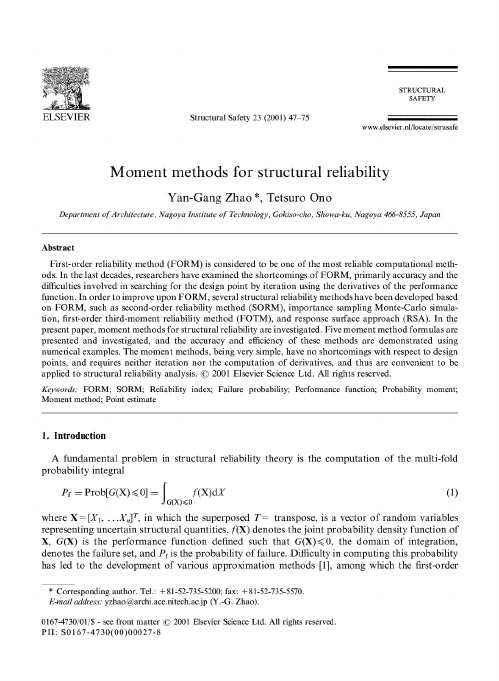
Department of Architecture, Nagoya Institute of Technology, Gokiso-cho, Showa-ku, Nagoya 466-8555, Japan
Abstract F ir st-order reliability method (FORM) is considered to be one of the most reliable computational methods. In the last decades, researchers have examined the shortcomings of FORM, primarily accuracy and the difficulties involved in searching for the design point by iteration using the derivatives of the performance function. In o rde r to improve upon FORM, several structural reliability methods have been developed based on FORM, such as second-order reliability method (SORM), importance sampling Monte~Carlo simulation, first-order third-moment reliability method (FOTM), and response surface approach (RSA). In the present paper, moment methods for structural reliability are investigated. Five moment method formulas are presented a nd investigated, and the accuracy and efficiency of these methods are demonstrated using numerical examples. The moment methods, being very simple, have no shortcomings with respect to design points, and requires neither iteration nor the computation of derivatives, and thus are convenient to be applied to structural reliability analysis. © 2001 Elsevier Science L td. All rights reserved.

New Perspectives on the Structure of Graphitic Carbons

Critical Reviews in Solid State and Materials Sciences,30:235–253,2005 Copyright c Taylor and Francis Inc.ISSN:1040-8436printDOI:10.1080/10408430500406265New Perspectives on the Structure of Graphitic CarbonsPeter J.F.Harris∗Centre for Advanced Microscopy,University of Reading,Whiteknights,Reading,RG66AF,UKGraphitic forms of carbon are important in a wide variety of applications,ranging from pollutioncontrol to composite materials,yet the structure of these carbons at the molecular level ispoorly understood.The discovery of fullerenes and fullerene-related structures such as carbonnanotubes has given a new perspective on the structure of solid carbon.This review aims toshow how the new knowledge gained as a result of research on fullerene-related carbons canbe applied to well-known forms of carbon such as microporous carbon,glassy carbon,carbonﬁbers,and carbon black.Keywords fullerenes,carbon nanotubes,carbon nanoparticles,non-graphitizing carbons,microporous carbon,glassy carbon,carbon black,carbonﬁbers.Table of Contents INTRODUCTION (235)FULLERENES,CARBON NANOTUBES,AND CARBON NANOPARTICLES (236)MICROPOROUS(NON-GRAPHITIZING)CARBONS (239)Background (239)Early Models (241)Evidence for Fullerene-Like Structures in Microporous Carbons (242)New Models for the Structure of Microporous Carbons (242)Carbonization and the Structural Evolution of Microporous Carbon (243)GLASSY CARBON (244)CARBON FIBERS (245)CARBON BLACK (248)Background (248)Structure of Carbon Black Particles (249)Effect of High-Temperature Heat Treatment on Carbon Black Structure (250)CONCLUSIONS (250)ACKNOWLEDGMENTS (251)REFERENCES (251)INTRODUCTIONUntil quite recently we knew for certain of just two allotropes of carbon:diamond and graphite.The vast range of carbon ma-∗E-mail:p.j.f.harris@ terials,both natural and synthetic,which have more disordered structures have traditionally been considered as variants of one or other of these two allotropes.Because the great majority of these materials contain sp2carbon rather than sp3carbon,their struc-tures have been thought of as being made up from tiny fragments235236P.J.F.HARRISFI G.1.(a)Model of PAN-derived carbon ﬁbres from the work of Crawford and Johnson,1(b)model of a non-graphitizing carbon by Ban and colleagues.2of crystalline graphite.Examples of models for the structures of carbons in which the basic elements are graphitic are reproduced in Figure 1.The structure shown in Figure 1(a)is a model for the structure of carbon ﬁbers suggested by Crawford and Johnson in 1971,1whereas 1(b)shows a model for non-graphitizing car-bon given by Ban and colleagues in 1975.2Both structures are constructed from bent or curved sheets of graphite,containing exclusively hexagonal rings.Although these models probably provide a good ﬁrst approximation of the structures of these car-bons,in many cases they fail to explain fully the properties of the materials.Consider the example of non-graphitizing carbons.As the name suggests,these cannot be transformed into crystalline graphite even at temperatures of 3000◦C and above.I nstead,high temperature heat treatments transform them into structures with a high degree of porosity but no long-range crystalline order.I n the model proposed by Ban et al.(Figure 1(b)),the structure is made up of ribbon-like sheets enclosing randomly shaped voids.It is most unlikely that such a structure could retain its poros-ity when subjected to high temperature heat treatment—surface energy would force the voids to collapse.The shortcomings of this and other “conventional”models are discussed more fully later in the article.The discovery of the fullerenes 3−5and subsequently of re-lated structures such as carbon nanotubes,6−8nanohorns,9,10and nanoparticles,11has given us a new paradigm for solid car-bon structures.We now know that carbons containing pentago-nal rings,as well as other non-six-membered rings,among the hexagonal sp 2carbon network,can be highly stable.This new perspective has prompted a number of groups to take a fresh look at well-known forms of carbon,to see whether any evidence can be found for the presence of fullerene-like structures.12−14The aim of this article is to review this new work on the structure of graphitic carbons,to assess whether models that incorporate fullerene-like elements could provide a better basis for under-standing these materials than the conventional models,and to point out areas where further work is needed.The carbon ma-terials considered include non-graphitizing carbon,glassy car-bon,carbon ﬁbers,and carbon black.The article begins with an outline of the main structural features of fullerenes,carbon nanotubes,and carbon nanoparticles,together with a brief dis-cussion of their stability.FULLERENES,CARBON NANOTUBES,AND CARBON NANOPARTICLESThe structure of C 60,the archetypal fullerene,is shown in Figure 2(a).The structure consists of twelve pentagonal rings and twenty hexagons in an icosahedral arrangement.I t will be noted that all the pentagons are isolated from each other.This is important,because adjacent pentagonal rings form an unstable bonding arrangement.All other closed-cage isomers of C 60,and all smaller fullerenes,are less stable than buck-minsterfullerene because they have adjacent pentagons.For higher fullerenes,the number of structures with isolated pen-tagonal rings increases rapidly with size.For example,C 100has 450isolated-pentagon isomers.16Most of these higher fullerenes have low symmetry;only a very small number of them have the icosahedral symmetry of C 60.An example of a giant fullerene that can have icosahedral symmetry is C 540,as shown in Figure 2(b).There have been many studies of the stability of fullerenes as a function of size (e.g.,Refs.17,18).These show that,in general,stability increases with size.Experimentally,there is evidence that C 60is unstable with respect to large,multiwalled fullerenes.This was demonstrated by Mochida and colleagues,who heated C 60and C 70in a sublimation-limiting furnace.19They showed that the cage structure broke down at 900◦C–1000◦C,although at 2400◦C fullerene-like “hollow spheres”with diameters in the range 10–20nm were formed.We now consider fullerene-related carbon nanotubes,which were discovered by Iijima in 1991.6These consist of cylinders of graphite,closed at each end with caps that contain precisely six pentagonal rings.We can illustrate their structure by considering the two “archetypal”carbon nanotubes that can be formed by cutting a C 60molecule in half and placing a graphene cylinder between the two halves.Dividing C 60parallel to one of the three-fold axes results in the zig-zag nanotube shown in Figure 3(a),whereas bisecting C 60along one of the ﬁvefold axes produces the armchair nanotube shown in Figure 3(b).The terms “zig-zag”and “armchair”refer to the arrangement of hexagons around the circumference.There is a third class of structure in which the hexagons are arranged helically around the tube axis.Ex-perimentally,the tubes are generally much less perfect than the idealized versions shown in Figure 3,and may be eitherNEW PERSPECTIVES ON GRAPHITIC CARBONS STRUCTURE237FI G.2.The structure of (a)C 60,(b)icosahedral C 540.15multilayered or single-layered.Figure 4shows a high resolu-tion TEM image of multilayered nanotubes.The multilayered tubes range in length from a few tens of nm to several microns,and in outer diameter from about 2.5nm to 30nm.The end-caps of the tubes are sometimes symmetrical in shape,but more often asymmetric.Conical structures of the kind shown in Fig-ure 5(a)are commonly observed.This type of structure is be-lieved to result from the presence of a single pentagon at the position indicated by the arrow,with ﬁve further pentagons at the apex of the cone.Also quite common are complex cap struc-tures displaying a “bill-like”morphology such as thatshownFI G.3.Drawings of the two nanotubes that can be capped by one half of a C 60molecule.(a)Zig-zag (9,0)structure,(b)armchair (5,5)structure.20in Figure 5(b).21This structure results from the presence of a single pentagon at point “X”and a heptagon at point “Y .”The heptagon results in a saddle-point,or region of negative curvature.The nanotubes ﬁrst reported by Iijima were prepared by va-porizing graphite in a carbon arc under an atmosphere of helium.Nanotubes produced in this way are invariably accompanied by other material,notably carbon nanoparticles.These can be thought of as giant,multilayered fullerenes,and range in size from ∼5nm to ∼15nm.A high-resolution image of a nanopar-ticle attached to a nanotube is shown in Figure 6(a).22In this238P.J.F.HARRISFI G.4.TEM image of multiwalled nanotubes.case,the particle consists of three concentric fullerene shells.A more typical nanoparticle,with many more layers,is shown in Figure 6(b).These larger particles are probably relatively im-perfect instructure.FI G.5.I mages of typical multiwalled nanotube caps.(a)cap with asymmetric cone structure,(b)cap with bill-like structure.21Single-walled nanotubes were ﬁrst prepared in 1993using a variant of the arc-evaporation technique.23,24These are quite different from multilayered nanotubes in that they generally have very small diameters (typically ∼1nm),and tend to be curledNEW PERSPECTIVES ON GRAPHITIC CARBONS STRUCTURE239FI G.6.I mages of carbon nanoparticles.(a)small nanoparticle with three concentric layers on nanotube surface,22(b)larger multilayered nanoparticle.and looped rather than straight.They will not be considered further here because they have no parallel among well-known forms of carbon discussed in this article.The stability of multilayered carbon nanotubes and nanopar-ticles has not been studied in detail experimentally.However,we know that they are formed at the center of graphite electrodes during arcing,where temperatures probably approach 3000◦C.I t is reasonable to assume,therefore,that nanotubes and nanopar-ticles could withstand being re-heated to such temperatures (in an inert atmosphere)without signiﬁcant change.MICROPOROUS (NON-GRAPHITIZING)CARBONS BackgroundIt was demonstrated many years ago by Franklin 25,26that carbons produced by the solid-phase pyrolysis of organic ma-terials fall into two distinct classes.The so-called graphitizing carbons tend to be soft and non-porous,with relatively high den-sities,and can be readily transformed into crystalline graphite by heating at temperatures in the range 2200◦C–3000◦C.I n con-trast,“non-graphitizing”carbons are hard,low-densitymateri-FI G.7.(a)High resolution TEM image of carbon prepared by pyrolysis of sucrose in nitrogen at 1000◦C,(b)carbon prepared bypyrolysis of anthracene at 1000◦C.I nsets show selected area diffraction patterns.30als that cannot be transformed into crystalline graphite even at temperatures of 3000◦C and above.The low density of non-graphitizing carbons is a consequence of a microporous struc-ture,which gives these materials an exceptionally high internal surface area.This high surface area can be enhanced further by activation,that is,mild oxidation with a gas or chemical pro-cessing,and the resulting “activated carbons”are of enormous commercial importance,primarily as adsorbents.27−29The distinction between graphitizing and non-graphitizing carbons can be illustrated most clearly using transmission elec-tron microscopy (TEM).Figure 7(a)shows a TEM image of a typical non-graphitizing carbon prepared by the pyrolysis of sucrose in an inert atmosphere at 1000◦C.30The inset shows a diffraction pattern recorded from an area approximately 0.25µm in diameter.The image shows the structure to be disordered and isotropic,consisting of tightly curled single carbon layers,with no obvious graphitization.The diffraction pattern shows symmetrical rings,conﬁrming the isotropic structure.The ap-pearance of graphitizing carbons,on the other hand,approxi-mates much more closely to that of graphite.This can be seen in the TEM micrograph of a carbon prepared from anthracene,240P.J.F.HARRI Swhich is shown in Figure 7(b).Here,the structure contains small,approximately ﬂat carbon layers,packed tightly together with a high degree of alignment.The fragments can be considered as rather imperfect graphene sheets.The diffraction pattern for the graphitizing carbon consists of arcs rather than symmetrical rings,conﬁrming that the layers are preferentially aligned along a particular direction.The bright,narrow arcs in this pattern correspond to the interlayer {0002}spacings,whereas the other reﬂections appear as broader,less intense arcs.Transmission electron micrographs showing the effect of high-temperature heat treatments on the structure of non-graphitizing and graphitizing carbons are shown in Figure 8(note that the magniﬁcation here is much lower than for Figure 7).I n the case of the non-graphitizing carbon,heating at 2300◦C in an inert atmosphere produces the disordered,porous material shown in Figure 8(a).This structure is made up of curved and faceted graphitic layer planes,typically 1–2nm thick and 5–15nm in length,enclosing randomly shaped pores.A few somewhat larger graphite crystallites are present,but there is no macroscopic graphitization.n contrast,heat treatment of the anthracene-derived carbon produces large crystals of highly or-dered graphite,as shown in Figure 8(b).Other physical measurements also demonstrate sharp dif-ferences between graphitizing and non-graphitizing carbons.Table 1shows the effect of preparation temperature on the sur-face areas and densities of a typical graphitizing carbon prepared from polyvinyl chloride,and a non-graphitizing carbon prepared from cellulose.31It can be seen that the graphitizing carbon pre-pared at 700◦C has a very low surface area,which changes lit-tle for carbons prepared at higher temperatures,up to 3000◦C.The density of the carbons increases steadily as thepreparationFI G.8.Micrographs of (a)sucrose carbon and (b)anthracene carbon following heat treatment at 2300◦C.TABLE 1Effect of temperature on surface areas and densities of carbonsprepared from polyvinyl chloride and cellulose 31(a)Surface areas Speciﬁc surface area (m 2/g)for carbons prepared at:Starting material 700◦C 1500◦C 2000◦C 2700◦C 3000◦C PVC 0.580.210.210.710.56Cellulose 4081.601.172.232.25(b)Densities Helium density (g/cm 3)for carbons prepared at:Starting material 700◦C 1500◦C 2000◦C 2700◦C 3000◦C PVC 1.85 2.09 2.14 2.21 2.26Cellulose1.901.471.431.561.70temperature is increased,reaching a value of 2.26g/cm 3,which is the density of pure graphite,at 3000◦C.The effect of prepara-tion temperature on the non-graphitizing carbon is very different.A high surface area is observed for the carbon prepared at 700◦C (408m 2/g),which falls rapidly as the preparation temperature is increased.Despite this reduction in surface area,however,the density of the non-graphitizing carbon actually falls when the temperature of preparation is increased.This indicates that a high proportion of “closed porosity”is present in the heat-treated carbon.NEW PERSPECTIVES ON GRAPHITIC CARBONS STRUCTURE241FI G.9.Franklin’s representations of(a)non-graphitizing and(b)graphitizing carbons.25Early ModelsTheﬁrst attempt to develop structural models of graphitizingand non-graphitizing carbons was made by Franklin in her1951paper.25In these models,the basic units are small graphitic crys-tallites containing a few layer planes,which are joined togetherby crosslinks.The precise nature of the crosslinks is not speci-ﬁed.An illustration of Franklin’s models is shown in Figure9.Using these models,she put forward an explanation of whynon-graphitizing carbons cannot be converted by heat treatmentinto graphite,and this will now be summarized.During car-bonization the incipient stacking of the graphene sheets in thenon-graphitizing carbon is largely prevented.At this stage thepresence of crosslinks,internal hydrogen,and the viscosity ofthe material is crucial.The resulting structure of the carbon(at ∼1000◦C)consists of randomly ordered crystallites,held to-gether by residual crosslinks and van der Waals forces,as inFigure9(a).During high-temperature treatment,even thoughthese crosslinks may be broken,the activation energy for themotion of entire crystallites,required for achieving the struc-ture of graphite,is too high and graphite is not formed.Onthe other hand,the structural units in a graphitizing carbon areapproximately parallel to each other,as in Figure9(b),and thetransformation of such a structure into crystalline graphite wouldbe expected to be relatively facile.Although Franklin’s ideason graphitizing and non-graphitizing carbons may be broadlycorrect,they are in some regards incomplete.For example,thenature of the crosslinks between the graphitic fragments is notspeciﬁed,so the reasons for the sharply differing properties ofgraphitizing and non-graphitizing carbons is not explained.The advent of high-resolution transmission electron mi-croscopy in the early1970s enabled the structure of non-graphitizing carbons to be imaged directly.n a typical study,Ban,Crawford,and Marsh2examined carbons prepared frompolyvinylidene chloride(PVDC)following heat treatments attemperatures in the range530◦C–2700◦C.I mages of these car-bons apparently showed the presence of curved and twistedgraphite sheets,typically two or three layer planes thick,enclos-ing voids.These images led Ban et al.to suggest that heat-treatednon-graphitizing carbons have a ribbon-like structure,as shownin Figure1(b).This structure corresponds to a PVDC carbonheat treated at1950◦C.This ribbon-like model is rather similar to an earlier model of glassy carbon proposed by Jenkins andKawamura.32However,models of this kind,which are intendedto represent the structure of non-graphitizing carbons follow-ing high-temperature heat treatment,have serious weaknesses,as noted earlier.Such models consist of curved and twistedgraphene sheets enclosing irregularly shaped pores.However,graphene sheets are known to be highlyﬂexible,and wouldtherefore be expected to become ever more closely folded to-gether at high temperatures,in order to reduce surface energy.Indeed,tightly folded graphene sheets are quite frequently seenin carbons that have been exposed to extreme conditions.33Thus,structures like the one shown in Figure1(b)would be unlikelyto be stable at very high temperatures.It has also been pointed out by Oberlin34,35that the modelsput forward by Jenkins,Ban,and their colleagues were basedon a questionable interpretation of the electron micrographs.In most micrographs of partially graphitized carbons,only the {0002}fringes are resolved,and these are only visible when they are approximately parallel to the electron beam.Therefore,such images tend to have a ribbon-like appearance.However,because only a part of the structure is being imaged,this appear-ance can be misleading,and the true three-dimensional structuremay be more cagelike than ribbon-like.This is a very importantpoint,and must always be borne in mind when analyzing imagesof graphitic carbons.Oberlin herself believes that all graphiticcarbons are built up from basic structural units,which comprisesmall groups of planar aromatic structures,35but does not appearto have given a detailed explanation for the non-graphitizabilityof certain carbons.The models of non-graphitizing carbons described so farhave assumed that the carbon atoms are exclusively sp2and arebonded in hexagonal rings.Some authors have suggested thatsp3-bonded atoms may be present in these carbons(e.g.,Refs.36,37),basing their arguments on an analysis of X-ray diffrac-tion patterns.The presence of diamond-like domains would beconsistent with the hardness of non-graphitizing carbons,andmight also explain their extreme resistance to graphitization.Aserious problem with these models is that sp3carbon is unsta-ble at high temperatures.Diamond is converted to graphite at1700◦C,whereas tetrahedrally bonded carbon atoms in amor-phousﬁlms are unstable above about700◦C.Therefore,the242P.J.F.HARRI Spresence of sp 3atoms in a carbon cannot explain the resistance of the carbon to graphitization at high temperatures.I t should also be noted that more recent diffraction studies of non-graphitizing carbons have suggested that sp 3-bonded atoms are not present,as discussed further in what follows.Evidence for Fullerene-Like Structures in Microporous CarbonsThe evidence that microporous carbons might have fullerene-related structures has come mainly from high-resolution TEM studies.The present author and colleagues initiated a series of studies of typical non-graphitizing microporous carbons using this technique in the mid 1990s.30,38,39The ﬁrst such study in-volved examining carbons prepared from PVDC and sucrose,after heat treatments at temperatures in the range 2100◦C–2600◦C.38The carbons subjected to very high temperatures had rather disordered structures similar to that shown in Figure 8(a).Careful examination of the heated carbons showed that they often contained closed nanoparticles;examples can be seen in Figure 10.The particles were usually faceted,and often hexagonal or pentagonal in shape.Sometimes,faceted layer planes enclosed two or more of the nanoparticles,as shown in Figure 10(b).Here,the arrows indicate two saddle-points,similar to that shown in Figure 5(b).The closed nature of the nanoparticles,their hexagonal or pentagonal shapes,and other features such as the saddle-points strongly suggest that the parti-cles have fullerene-like structures.I ndeed,in many cases the par-ticles resemble those produced by arc-evaporation in a fullerene generator (see Figure 6)although in the latter case the particles usually contain many more layers.The observation of fullerene-related nanoparticles in the heat treated carbons suggested that the original,freshly prepared car-bons may also have had fullerene-related structures (see next section).However,obtaining direct evidence for this is difﬁ-cult.High resolution electron micrographs of freshly prepared carbons,such as that shown in Figure 7(a),are usuallyratherFI G.10.(a)Micrograph showing closed structure in PVDC-derived carbon heated at 2600◦C,(b)another micrograph of same sample,with arrows showing regions of negative curvature.38featureless,and do not reveal the detailed structure.Occasion-ally,however,very small closed particles can be found in the carbons.30The presence of such particles provides circumstan-tial evidence that the surrounding carbon may have a fullerene-related structure.Direct imaging of pentagonal rings by HRTEM has not yet been achieved,but recent developments in TEM imaging techniques suggest that this may soon be possible,as discussed in the Conclusions.As well as high-resolution TEM,diffraction methods have been widely applied to microporous and activated carbons (e.g.,Refs.40–44).However,the interpretation of diffraction data from these highly disordered materials is not straightforward.As already mentioned,some early X-ray diffraction studies were interpreted as providing evidence for the presence of sp 3-bonded atoms.More recent neutron diffraction studies have suggested that non-graphitizing carbons consist entirely of sp 2atoms.40It is less clear whether diffraction methods can establish whether the atoms are bonded in pentagonal or hexagonal rings.Both Petkov et al .42and Zetterstrom and colleagues 43have interpreted neutron diffraction data from nanoporous carbons in terms of a structure containing non-hexagonal rings,but other interpreta-tions may also be possible.Raman spectroscopy is another valuable technique for the study of carbons.45Burian and Dore have used this method to analyze carbons prepared from sucrose,heat treated at tem-peratures from 1000◦C–2300◦C.46The Raman spectra showed clear evidence for the presence of fullerene-and nanotube-like elements in the carbons.There was also some evidence for fullerene-like structures in graphitizing carbons prepared from anthracene,but these formed at higher temperatures and in much lower proportions than in the non-graphitizing carbons.New Models for the Structure of Microporous Carbons Prompted by the observations described in the previous section,the present author and colleagues proposed a model for the structure of non-graphitizing carbons that consists ofNEW PERSPECTIVES ON GRAPHITIC CARBONS STRUCTURE243FI G.11.Schematic illustration of a model for the structure of non-graphitizing carbons based on fullerene-like elements.discrete fragments of curved carbon sheets,in which pentagons and heptagons are dispersed randomly throughout networks of hexagons,as illustrated in Figure11.38,39The size of the micropores in this model would be of the order of0.5–1.0nm, which is similar to the pore sizes observed in typical microp-orous carbons.The structure has some similarities to the“ran-dom schwarzite”network put forward by Townsend and col-leagues in1992,47although this was not proposed as a model for non-graphitizing carbons.I f the model we have proposed for non-graphitizing carbons is correct it suggests that these carbons are very similar in structure to fullerene soot,the low-density, disordered material that forms on walls of the arc-evaporation vessel and from which C60and other fullerenes may be ex-tracted.Fullerene soot is known to be microporous,with a sur-face area,after activation with carbon dioxide,of approximately 700m2g−1,48and detailed analysis of high resolution TEM mi-crographs of fullerene soot has shown that these are consis-tent with a structure in which pentagons and heptagons are dis-tributed randomly throughout a network of hexagons.49,50It is signiﬁcant that high-temperature heat treatments can transform fullerene soot into nanoparticles very similar to those observed in heated microporous carbon.51,52Carbonization and the Structural Evolutionof Microporous CarbonThe process whereby organic materials are transformed into carbon by heat treatment is not well understood at the atomic level.53,54In particular,the very basic question of why some organic materials produce graphitizing carbons and others yield non-graphitizing carbons has not been satisfactorily answered. It is known,however,that both the chemistry and physical prop-erties of the precursors are important in determining the class of carbon formed.Thus,non-graphitizing carbons are formed, in general,from substances containing less hydrogen and more oxygen than graphitizing carbons.As far as physical properties are concerned,materials that yield graphitizing carbons usu-ally form a liquid on heating to temperatures around400◦C–500◦C,whereas those that yield non-graphitizing carbons gen-erally form solid chars without melting.The liquid phase pro-duced on heating graphitizing carbons is believed to provide the mobility necessary to form oriented regions.However,this may not be a complete explanation,because some precursors form non-graphitizing carbons despite passing through a liquid phase.The idea that non-graphitizing carbons contain pentagons and other non-six-membered rings,whereas graphitizing car-bons consist entirely of hexagonal rings may help in understand-ing more fully the mechanism of carbonization.Recently Kumar et al.have used Monte Carlo(MC)simulations to model the evo-lution of a polymer structure into a microporous carbon structure containing non-hexagonal rings.55They chose polyfurfuryl al-cohol,a well-known precursor for non-graphitizing carbon,as the starting material.The polymer was represented as a cubic lattice decorated with the repeat units,as shown in Figure12(a). All the non-carbon atoms(i.e.,hydrogen and oxygen)were then removed from the polymer and this network was used in the。

计量经济学中英文词汇对照

Controlled experiments Conventional depth Convolution Corrected factor Corrected mean Correction coefficient Correctness Correlation coefficient Correlation index Correspondence Counting Counts Covaห้องสมุดไป่ตู้iance Covariant Cox Regression Criteria for fitting Criteria of least squares Critical ratio Critical region Critical value
Asymmetric distribution Asymptotic bias Asymptotic efficiency Asymptotic variance Attributable risk Attribute data Attribution Autocorrelation Autocorrelation of residuals Average Average confidence interval length Average growth rate BBB Bar chart Bar graph Base period Bayes' theorem Bell-shaped curve Bernoulli distribution Best-trim estimator Bias Binary logistic regression Binomial distribution Bisquare Bivariate Correlate Bivariate normal distribution Bivariate normal population Biweight interval Biweight M-estimator Block BMDP(Biomedical computer programs) Boxplots Breakdown bound CCC Canonical correlation Caption Case-control study Categorical variable Catenary Cauchy distribution Cause-and-effect relationship Cell Censoring

mixsim帮助

MIXSIM2.1Tutorial November2006Copyright c 2006by Fluent Inc.All Rights Reserved.No part of this document may be reproduced or otherwise used in any form without express written permission from Fluent Inc.Airpak,FIDAP,FLUENT,FLUENT for CATIA V5,FloWizard,GAMBIT,Icemax,Icepak, Icepro,Icewave,Icechip,MixSim,and POLYFLOW are registered trademarks of Fluent Inc.All other products or name brands are trademarks of their respective holders.CHEMKIN is a registered trademark of Reaction Design Inc.Portions of this program include material copyrighted by PathScale Corporation2003-2004.Fluent Inc.Centerra Resource Park10Cavendish CourtLebanon,NH03766Tutorial:Cylindrical Vessel with a Pitched Blade Impeller and Flat BaﬄesIntroductionThe purpose of this tutorial is to introduce to you,the MixSim2.1user interface and the typical problem-solving procedure.It illustrates the setup and solution of a simple mixer conﬁguration consisting of a cylindrical vessel with a pitched blade impeller and four baﬄes.This conﬁguration is commonly used in process industries for mixing and related operations.This tutorial demonstrates how to do the following:•Create a new model.•Specify theﬂuid and its relevant properties.•Deﬁne the tank,baﬄes,shaft,and impeller geometry.•Generate the grid.•Perform the calculation.•Postprocess the results.PrerequisitesThis tutorial assumes that you have read Chapters3and4of the MixSim User’s Guide and are familiar with the basic user interface elements.Problem DescriptionThe conﬁguration considered in this tutorial is shown in Figure1.The cylindrical tank, with an ASME10%tank bottom shape,has a diameter of1.0m,a liquid level height of1.0m,and an open top.This means that the top shape of the tank is not speciﬁed,becausethe liquid level remains in the cylindrical part of the tank.The tank contains a top mounted,centrally located shaft,a pitched blade axialﬂow impeller mounted to it,and fourﬂat baﬄes.Theﬂuid in the tank is water.The liquidﬂowﬁeld is solved and displayed during postprocessing.c Fluent Inc.November3,20061Cylindrical Vessel with a Pitched Blade Impeller and Flat BaﬄesFigure1:Problem SchematicStep1:Starting a New Session1.Start MixSim.2.Create a new model.File−→New ModelThe Model Management panel and a graphics display window will open.The modeldetails and geometry are deﬁned in the Model Management panel.This panel containsan Object Tree,Graphics Display,and some text-entry boxes.The graphics displaywindow shows three views of the geometry:front view,top view,and a view that youcan manipulate.Arrange these windows on your screen so that both are visible.2c Fluent Inc.November3,2006Cylindrical Vessel with a Pitched Blade Impeller and Flat Baﬄes3.Specify an appropriate title and a brief description in the Title and Descriptionﬁelds,respectively.The text entered in the Title and Descriptionﬁelds appears only in the the Model Management panel(here)and at the top of the generated HTML report.4.Enter cyl-pitched-blade for File Name.Thisﬁle name will be used as a preﬁx for allﬁles that are automatically created by MixSim,(mesh and dataﬁles).c Fluent Inc.November3,20063Cylindrical Vessel with a Pitched Blade Impeller and Flat Baﬄes5.Retain the selection of MRF in the Analysis Type drop-down list.6.Click Apply to save your inputs.You need to click Apply to save your inputs after modifying any entry in the ModelManagement panel.Step2:Fluid PropertiesYou need not visit the Continuum panel if you plan to run the simulation with the default settings.You can directly set theﬂuid material.Here,we introduce to you the interface ele-ments that can be used to choose diﬀerent settings for the turbulance model and/ot material properties.1.Select Continuum in the Object Tree.The Model Management panel will show a set of buttons for handling materials andrelated models.2.Click the Viscous Model button to open the Viscous Model panel.You can specify either laminar or turbulentﬂow in the Viscous Model panel.You canselect the turbulence model to be used.The default Realizable k-epsilon model is usedin this example.(a)Retain the default selection of k-epsilon(2eqn)in the Model list and Realizablein the k-epsilon Model list,respectively.(b)Click OK to close the Viscous Model panel.(c)Click Apply in the Model Management panel to save the settings.4c Fluent Inc.November3,2006Cylindrical Vessel with a Pitched Blade Impeller and Flat Baﬄes Two more buttons(Edit Materials and Copy Material)are provided in the Continuum object panel.They allow you to copy one or more materials from a database into the MixSim session and edit(modify)them.For more information on using the Mate-rials panel and adding new materials to the database,refer to Section6.3:Physical Properties in the MixSim User’s Guide.3.Select water-liquid as theﬂuid material for this model.(a)Select Fluid in the Object Tree.(b)Retain the default material,water-liquid for your model.(c)Click Apply in the Model Management panel to save water-liquid as theﬂuid forthis model.Select a suitable material in the Material Selection panel to run the simulation with some otherﬂuid(in the tank).Click the Select Material...button in the Fluid section to open the Material Selection panel.Step3:Tank1.Select Cylindrical Tank in the Object Tree.The Model Management panel will now display the parameters required to deﬁne the cylindrical tank.To the right of the panel is a list of object buttons in the Add Object group box.c Fluent Inc.November3,20065Cylindrical Vessel with a Pitched Blade Impeller and Flat Baﬄes2.Retain the default values for Diameter,Tank Height,and Liquid Level of the tank.3.Retain the selection of Open in the Top Style drop-down list.4.Select ASME(10%)in the Bottom Style drop-down list.5.Retain other default settings and click Apply.The graphics display in the Model Management panel and graphics window are updatedto display the tank according to your speciﬁcations.You can manipulate the view inthe top right frame of the preview graphics window.You can rotate the image usingthe left mouse button,zoom the image using the right mouse button and center theimage in the window using the middle mouse button.6c Fluent Inc.November3,2006Cylindrical Vessel with a Pitched Blade Impeller and Flat BaﬄesFigure2:Cylindrical Tank with ASME10%Bottom StyleStep4:Baﬄes1.Click Baﬄe in the Add Object group box.A Baﬄe frame with a list of diﬀerent types of baﬄes is displayed.2.Click Flat Baﬄes in the Baﬄe frame.The Model Management panel will now display the parameters for theﬂat baﬄes.c Fluent Inc.November3,20067Cylindrical Vessel with a Pitched Blade Impeller and Flat Baﬄes3.Retain0.194m for Bottom Elevation.4.Enter1.1for Top Elevation.This will allow the baﬄes to extend to the top of the tank.5.Retain the default value of0.1m for Width and Distance from Wall.6.Make sure that the Zero Thickness Baﬄe option is enabled.Note:MixSim will neglect the baﬄe thickness in the simulated geometry and compu-tational grid when the Zero Thickness Baﬄe option is enabled.This will reducethe number of computational cells and hence,the memory(RAM)and calculationtime for the solution,without signiﬁcantly aﬀecting the accuracy of the results.7.Retain the default values for other parameters and click Apply.The graphics window is updated to display the tank with the baﬄes(Figure3).8c Fluent Inc.November3,2006Figure3:Tank with Flat BaﬄesStep5:Shaft1.Click Cylindrical Tank in the Object Tree.To add another“child”object to the vessel,you must go back to the parent object.2.Click Shaft in the Add Object group box.A Shaft frame with a list of diﬀerent types of shafts will be displayed.3.Click Top Shaft in the Shaft frame.The Model Management panel will now display the parameters required to deﬁne the top shaft.4.Enter150rpm for Speed.5.Enter0.3m for Shaft Tip Elevation and click Apply.The graphics window is updated to display the tank with the baﬄes and the shaft.Figure4:Tank with Baﬄes and ShaftStep6:Impeller1.Click Generic Impellers in the Add Object group box.A Generic Impellers frame with a list of diﬀerent impeller models will be displayed.2.Click the Pitched Blade button in the Generic Impellers frame.The Model Management panel will now display the parameters required to deﬁne the Pitched Blade impeller.3.Enter0.35m for Diameter in order to resize the impeller to suit the tank dimensions.4.Enter0.35m for Axial Location.5.Retain other default parameters and click Apply.The graphics window is updated todisplay the tank with baﬄes,shaft,and impeller(Figure5).6.Close the Model Management panel.Figure 5:Tank with Baﬄes,Shaft,and Impeller7.Save the MixSim model.File−→Write−→MixSim Model...(a)Retain the suggestedﬁle name(cyl-pitched-blade.mxm)and click OK.The suggestedﬁle name in the Write:MixSim Model Fileﬁeld(cyl-pitched-blade.mxm) is automatically generated from the File Name parameter,entered in the Model Man-agement panel at the beginning of the session.Thisﬁle name is generated only once.If you change the File Name parameter after saving the model once,the suggestedﬁle name for Write:MixSim Model File will not change.Step7:Grid1.Generate the grid.Grid−→Generate Grid...MixSim uses the GAMBIT process in the background to create the geometry and gen-erate the grid.As the grid is generated,GAMBIT commands appear on the MixSim console and a progress bar panel will show the rate of completion of the grid generation process.When the geometry is created,MixSim saves the GAMBITﬁles.You can use these ﬁles to generate the mesh on your own or add custom objects using GAMBIT.When the grid is generated,it is automatically loaded into the FLUENT6.2component of MixSim.It is checked and statistics on the mesh skewness is reported in the MixSim console.Skewness is a measure of cell distortion as compared to a perfect cell of the same topology(tetrahedron,hexahedron,etc.).There should be few cells above the skewness of0.9.The grid for this model has a highest skewness value between0.8and0.85, and is acceptable.Cells with skewness values above0.95will slow down or may even impede convergence.An Information dialog box will appear,informing you that the meshing is complete.Click OK to close the Information dialog box and proceed.2.Display the grid.Display−→Grid...(a)Click Display to view the grid(Figure6)and close the MixSim Grid Display panel.The grid is displayed in a new graphics window.You can rotate the image using the left mouse button,zoom the image using the right mouse button and center the image in the window using the middle mouse button.You can also view the faces,feature edges and speciﬁc entities,using diﬀerent options in the Options,Edge Type and Surfaces lists.Figure6:Grid DisplayStep8:Solution1.Start the calculation.Solve−→IterateThe default number of iterations is10.2.Retain the number of initial iterations.MixSim sets up and runs the calculation using its FLUENT component.During the calculation,MixSim will display convergence monitor plots for turbulent kinetic energy (averaged on the free liquid surface),shaft moment(torque),and scaled residuals.These plots tell you when the solution hasﬁnished.When the(scaled)residuals are small and some representative quantities do not change(signiﬁcantly)between itera-tions any more,you may assume that the iterative solution has converged and more iterations will not improve the result further.The representative quantities are chosen and plotted automatically by MixSim,and are used for theﬁrst two monitor plots.The values of these monitor quantities usually take very large negative or positive values during theﬁrst few iterations and then rapidly approach a relatively narrow range close to theﬁnal value.Judging the relative change in these values from one iteration to the next is diﬃcult,because the interesting changes are squeezed vertically in the plots that still contain much higher initial values.To improve the plot around theﬁnal value,you should clear the plot after theﬁrst few iterations.For this reason, perform only10iterations when you begin the solution.For the guidelines on setting the number of iterations,see Section14.2.2in Chapter 14:Performing the Calculation.3.Click Iterate to start the calculation.The automatically created plot windows are shown in Figures7,8,and9.Figure7:Residual PlotFigure8:Convergence Plot forTurbulent Kinetic Energy4.Click the Reset Monitor Plot Data button in the Iterate panel.This resets the monitor plots.Otherwise,the automatic scaling of the ordinate axesin the monitor plots will cause the a part of the plot to be vertically compressed sothat no useful information can be seen.Solve−→Iterate(a)Click Reset Monitor Plot Data.5.Reset the number of iterations.Mixing tank models generally take approximately5000iterations to converge.Gener-ally,a mixing simulation is considered to be converged when both,the shaft torque/moment and the turbulence energy monitorsﬂatten out and the residuals areﬂat and below1·10−5.When the residuals fall below1·10−5and the monitorsﬂatten out,it is notnecessary for the scaled residuals to become constant/ﬂat.(a)Make sure that the Initialize option is disabled.(b)Enable the Save Case and Save Data options.This will make sure that the case and dataﬁles are saved in the working directoryat the end of the simulation.Alternatively,you can disable these options and savetheﬁles manually after the iterations have been completed.(c)Enter5000for Iterations and click Iterate.The residuals and monitor plots at the end of5000iterations are shown in Fig-ures10,11,and12.Completing5000iterations may take quite some time.If for a diﬀerent model,youﬁnd that the monitor quantities are constant after fewer(e.g.3000)itera-tions,click Cancel in the Working dialog box or type<Ctrl-C>in the MixSimconsole to interrupt the solver.Allow some time for the solver to process yourrequest for interruption.!To obtain an accurate solution perform the calculation using higher order discretiza-tion.To switch to higher order discretization,click the Switch to Higher Accuracybutton in the Iterate panel and continue iterations till the solution appears converged.Figure10:Residual PlotFigure11:Convergence Plots for Turbulent Kinetic EnergyFigure12:Moment Convergence History About the Z-axisStep9:PostprocessingYou can use the case and dataﬁles provided with this tutorial to proceed with the post-processing for this problem.To do so,start a new MixSim session,load(or read)the modelﬁle(cyl-pitched-blade.mxm)and then load the FLUENT case and dataﬁles pro-vided(cyl-pitched-blade.cas and cyl-pitched-blade.dat).1.Start a new MixSim session.2.Read the MixSim modelﬁle provided with this tutorial.File−→Read−→MixSim Model...Select cyl-pitched-blade.mxm from the Files list and click OK.3.Read the converged case and dataﬁles provided with this tutorial:File−→Read−→Case&Data...Select cyl-pitched-blade.cas from the Files list and click OK.4.Display velocity vectors that start from the impeller surface.Display−→Vectors...(a)Enter10for Scale and retain the setting of0for Skip.(b)Select the impeller surface pitched blade5top wall from the Surfaces selectionlist.(c)Retain other default parameters and click Display to plot the vectors(Figure13).You can conﬁrm that the impeller is rotating clockwise and pumping down.Note:You can manipulate the graphics display with the mouse in the same way as when you displayed the grid.Figure13:Vectors of Velocity Magnitude(d)Modify the vector display.i.Enable Lights On and Show Tank in the Options group box in the Vectorspanel.ii.Click Display.The tank geometry will be added to the display according to the parameters previously set in the MixSim Grid Display panel.iii.Modify the display of the tank geometry.A.Enable the Edges and Faces options in the MixSim Grid Display panel.B.Select Feature from the Edge Type list.C.Deselect all entries in the Surfaces list using the light gray button abovethe top right corner of the list.D.Click the Outline button(below the Surfaces list).E.Click Display to make these choices eﬀective.F.Close the MixSim Grid Display panel.iv.Click Display in the Vectors panel to plot the modiﬁed view(Figure14).The changes you made in the MixSim Grid Display panel are reﬂected(see Figure14),but the tank is automatically cut open in the display,so that you can see all its internals.v.Close the Vectors panel.Figure14:Modiﬁed View of Vectors of Velocity Magnitude5.Display contours of static pressure.Display−→Contours...(a)Selectﬂat baﬄes6wall in the Surfaces list.(b)Enable Lights On,Show Tank,and Clear Colors in the Options group box.(c)Retain all other default values and click Display(Figure15).You can now see the contours of pressure on one side of the baﬄe.The pressure distribution on some baﬄes is on the side which is not facing you and there is a uniform grey color on the other side.Figure15:Contours of Static Pressure on Flat Baﬄes—View1(d)Select the other side of the baﬄes(ﬂat baﬄes6wall-shadow)from the Surfaceslist and click Display(Figure16)to view the pressure distribution on all the baﬄes facing you.Figure16:Contours of Static Pressure on Flat Baﬄes—View26.Create tank and impeller surfaces for postprocessing.Postprocessing−→Impeller Surfaces...(a)Select pitched blade5top and Tank in the Impeller List.(b)Click Create and close the Create Surfaces panel.MixSim will create three surfaces that surround the impeller,and a number of vertical cut planes through the tank at diﬀerent angles.You can display vectors and contours of variables on these surfaces.7.Display contours of velocity in the ﬂuid domain.Display −→Contours...(a)Select Velocity and Velocity Magnitude from the Contours of drop-down lists.(b)Deselect the previously selected surfaces and select tank cut plane 60degree fromthe Surfaces selection list.(c)Disable the Lights On option and click Display to display the contours of velocityin the ﬂuid domain (Figure 17).Figure 17:Contours of Velocity in the Fluid Domain8.Display velocity vectors on the vertical cut plane tank cut points 60degree (Figure 18).Figure 18:Velocity Vectors on the Cut PlaneYou can try increasing the Scale setting in the MixSim Velocity Vectors panel.9.Display the isosurface of velocity magnitude.Postprocessing−→Iso Surface...(a)Select Velocity and Velocity Magnitude from the Surface of Constant drop-downlists and click Compute.The isovalues for Velocity Magnitude will be displayed in the Min and Maxﬁelds.(b)Disable Faces in the Options group box in the MixSim Grid Display panel.Display−→Grid...(c)Move the Iso-Values slider from left to right to vary the isovalue from minimumto maximum(Figure19).Figure19:Isosurface of Velocity MagnitudeAs you move the slider,the graphics display is simultaneously updated.Thiswill help you in judging which part of the tank is poorly agitated.View thegraphic display simultaneously to see the isosurface for the corresponding isovalue(Figure19).10.Create a horizontal cut plane surface that is located exactly in the impeller plane.You need to switch to the FLUENT user interface.File−→Control Panel...(a)Select Fluent from the Switch GUI menubar list.(b)Close the Application Control Panel.You will now have access to the FLUENT menu bar and all the commands inFLUENT.(c)Open the Iso-Surface panel in FLUENT.Surface−→Iso-Surface...i.Select Grid...and Z-Coordinate from the Surface of Constant drop-down lists.ii.Click Compute.MixSim computes and displays the total range of z coordinate values.iii.Enter0.35(the z coordinate of the horizontal impeller plane)for Iso-Values.iv.Enter z=0.35in the New Surface Nameﬁeld.v.Click Create and close the Iso-Surface panel.(d)Switch back to the MixSim interface.File−→Control Panel...i.Select Mixsim from the Switch GUI menubar list.ii.Close the Application Control Panel.(e)Deselect the previously selected surfaces and select z=0.35from the Surfaces listin the Contours panel.(f)Enable Lights On,Show Tank,and Clear Colors in the Options group box.(g)Click Display(Figure20).Figure20:Contours of Velocity at the Impeller11.Display a sweep surface.Sweep surfaces allow you to dynamically create cut plane displays of contours or ve-locity vectors.Display−→Sweep Surface...(a)Select Contours in the Display Type list.The Contours panel will open.Click the Properties...button if the panel does notopen automatically.i.Select Pressure...and Static Pressure from the Contours of drop-down lists.ii.Select the surfaces on which you want to see a contour plot together with the sweep surface,e.g.the baﬄes.iii.Click Compute.MixSim will determine the minimum and maximum values for the chosenquantity that appear at any location of the selected surfaces.If you havenot selected any surface,the global maximum and minimum values will beidentiﬁed.If you want to specify the range of the color scale,disable AutoRange and enter appropriate values manually.iv.Click OK to close the Contours panel.(b)Move the horizontal slider located at the bottom of the Sweep Surface panel toview the surface sweeping throughout the tank domain(see Figures21,22,and23).(c)Enter1for the Final Value in the Animation group box.(d)Click the Animate button to animate the sweep surface.You will see the contour plot displayed at10successive planes.Notes:•Moving the slider automatically updates the graphics display.•All settings made in the MixSim Grid Display,Contours,or Vectors panels aﬀect the graphics display.•The Contours and Vectors panels can be accessed through the Properties button in the Sweep Surface panel.•To change the sweep direction,after entering vector component values in the X, Y,and Zﬁelds,press<Enter>on your keyboard while the cursor is placed in any of the X,Y,or Z entryﬁelds.Figure21:Contours of Pressure—Below the ImpellerFigure22:Contours of Pressure—At the ImpellerFigure23:Contours of Pressure—Above the ImpellerStep10:Generating ReportsIn addition to generating a correlations report,you can also create reports after the solution is complete.These results are calculated from the numericalﬂuidﬂow(CFD)simulation (not from any correlations).Reports can be generated using the options in the Report pull-down menu.1.Report torque and power consumption values for the impeller.Report−→Torque/PowerSelect a Shaft and an Impeller to automatically update the displayed values.The Update button allows you to force an update of the displayed values.See Chapter15:Examining the Solution for information on the other reports available in MixSim.2.Generate the HTML report for the MixSim model.Report−→Generic Reports(a)Select all the items in the Object List.(b)Enter an appropriateﬁle name in the File Nameﬁeld.You can use the Browse...button to select the location to save theﬁle.(c)Click Write.(d)View the report in the browser.The HTML report is shown in Figures24—28.The report has been split across pages for better viewability.The report will appear as a continuous page in the browser.Step11:Exit(a)Click Exit in the File menu to exit MixSim.File−→ExitFigure24:HTML Report—Geometry and Model Objects ListFigure25:HTML Report—Fluid PropertiesFigure26:HTML Report—Cylindrical Tank ParametersFigure27:HTML Report—Baﬄe and Shaft ParametersFigure28:HTML Report—Pitched Blade ParametersSummaryBy creating surfaces in theﬂuid domain,we can examine theﬂowﬁeld and can see high velocities in the region around and below the impeller,with the velocity sharply decreasing in the radial direction.Very low velocities exist near the baﬄes and directly below the impeller on the bottom of the vessel.These are theﬂow and velocity patterns expected in a mixing tank.This tutorial has illustrated a typical problem-solving procedure using MixSim and has also demonstrated the how to analyze the model using postprocessing tools.。

System using a polar coordinate stage and continuo

专利名称：System using a polar coordinate stage andcontinuous image rotation to compensatefor stage rotation发明人：Robert Buchanan,Richard A. Yarussi,Blaine R.Spady申请号：US09113484申请日：19980710公开号：US06320609B1公开日：20011120专利内容由知识产权出版社提供专利附图：摘要：A method for controlling a polar coordinate stage moves an object relative toan imaging system. While moving the object, the image of the object is rotated to compensate for rotation of the object. Accordingly, the orientations of features in the image are preserved, and removal of apparent rotation in the image reduces confusion an operator experiences while directing movement of the object. The angular velocity of the motion of the object is controlled so that image shift speed is independent of the radial position of the point being viewed. Use of a polar stage, reduces the required foot print for a stage and facilitates prealignment. In particular, an edge detector measures the position of the edge of the object while the polar coordinate stage rotates the object. A prealignment process determines the position and orientation of the object from the measured edge positions. A further alignment process uses automated pattern recognition which more easily identifies features on the object when the image is rotated so that the orientations of the feature are approximately known.申请人：NANOMETRICS INCORPORATED代理机构：Skjerven Morrill MacPherson LLP代理人：Brian D. Ogonowsky,Michael J. Halbert更多信息请下载全文后查看。

Filtered Historical Simulation

Filtering Historical Simulation.Backtest Analysis1By Giovanni Barone-Adesi, Kostas Giannopoulos and Les VosperMarch 2000A new generation of VaR models, based on historical simulation (boot-strapping), is being increasingly used in the risk management indus-try. It consists of generating scenarios, based on historical price changes, for all the variables in the portfolio. Since the estimated VaR is based on the empirical distribution of asset returns it re-flects a more realistic picture of the portfolio’s risk. Unfortu-nately this methodology has a number of disadvantages. To overcome some of them Barone-Adesi, Bourgoin and Giannopoulos(1998) and Bar-one-Adesi, Giannopoulos and Vosper (1999) introduce filtered histori-cal simulation (FHS hereafter). They take into account the changes in past and current volatilities of historical returns and make theleast number of assumptions about the statistical properties of fu-ture price changes.In this paper we backtest the FHS VaR model on three types of portfo-lios invested over a period of two years. The first set of backtests consists of LIFFE financial futures and options contracts traded on LIFFE. In the second set of backtests we examine the suitability of the FHS model on interest rate swaps. Finally, we backtest a set of mixed portfolios consisting of LIFFE interest rate futures and op-tions as well as plain vanilla swaps.We go beyond the strict criteria of the BIS recommendations by evalu-ating daily risk at four different confidence levels and five differ-ent trading horizons for a large number of realistic portfolios2 of derivative securities.In the first section we describe the backtesting methodology and re-port the results for the LIFFE portfolios. To enable us to appraise the different components of risk measurements on each of the three types of portfolios we run three sets of backtests, relaxing the fol-lowing assumptions in each test: in the first backtest we keep con-stant implied volatilities and FX rates. Our analysis focuses on how well FHS predicts losses due to futures and options market price changes. In our second backtest we simulate implied volatilitieswhile in the third backtest we also take into account the portfolios’FX exposure. Our results show that fixed implied volatility performs better at short VaR horizons, while at longer ones (5 to 10 days) our stochastic implied volatility performs better.1 Universita’ della Svizzera Italiana and City University Business School, Westminster Business School and London Clearing House. We are grateful to The London Clearing House for providing us the data and financing the project.2 For backtest 1, a total of 75,835 daily portfolios; backtests 2 and3 have a total of 75,985 portfolios.In the second series of backtests we investigate the performance of FHS on books of interest rate swaps. We compare each book’s daily values with the FHS lower forecasted value. For each book we produce two types of forecast; an aggregate market value risk expressed in GBP and a set of currency components (plain vanilla swaps in USD, JPY, DEM, and GBP are used). In the swap portfolios we find that our methodology is too conservative at longer horizons.In the final set of backtests we investigate the performance of the FHS model on diversified portfolios across plain vanilla swaps and futures and options traded on LIFFE. This study shares the same data with the separate LIFFE and Swaps backtests but restricts the number of portfolios to 20 among the largest members on LIFFE. By adding to each LIFFE portfolio one of the four swap books3 used in the swaps backtest we form 20 combined (combo) portfolios.Our analysis is based on two criteria: statistical and economic. The former examine the frequency and the pattern of losses exceeding the VaR predicted by FHS (breaks); the latter examine the implications of these breaks in economic terms, with reference to the total VaR allo-cated. Overall our findings sustain the validity of FHS as a risk measurement model. Furthermore, we find that diversification reduces risk effectively across the markets we study.3 Four SWAP books consisting of 500 Swaps each were formed for the SWAP backtest. Details of the portfolios are available from the authors.1 Overview of VaR models.VaR models play a core role in the risk management of today’s financial institutions. A number of VaR models are in use. All of them have the same aim, to measure the size of possible future losses at a predetermined probability. There are a variety of approaches used by VaR models to estimate the potential losses. Models differ in fact in the way they calculate the density function of future profits and losses of current positions, as well as the assumptions they rely on. Although VaR analysis has been used since early 1980’s by some departments of few large financial institutions it wasn’t until the middle 1990’s that it became widely accepted by banks and also imposed by the regulators. The cor-nerstone behind this wide acceptance was a linear VaR model, based on the variance-covariance of past security returns, introduced by JP Morgan, RiskMetrics (1993). The variance-covariance ap-proach to calculate risk can be traced back to the early days of Markowitz’s (1959) Modern Portfolio Theory, which is now common knowledge among today’s risk managers.Linear VaR models, however, impose strong assumptions about the underlying data. For example, the density function of daily returns follows a theoretical distribution (usually normal) and has constant mean and variance4. The empirical evidence about the distributional properties of speculative price changes provides evidence against these assumptions5, e.g. Kendall (1953) and Mandelbrot (1963). Risk managers have also seen their daily portfolio’s profits and losses to be much larger than those predicted by the normal distribution. The RiskMetrics VaR method has two additional major limita-tions. It linearises derivative positions and it does not take into account expiring contracts. These shortcomings may result in large biases, particularly for longer VaR horizons and for portfolios weighed with short out-of-the money options.To overcome problems of linearising derivative positions and to account for expiring contracts, risk managers have begun to look at simulation techniques. Pathways are simulated for scenarios for lin-ear positions, interest rate factors and currency exchange rate and are then used to value all positions for each scenario. The VaR is estimated from the distribution (e.g. 1st percentile) of the simulated portfolio values. Monte-Carlo simulation is widely used by financial institutions around the globe. Nevertheless, this method can attract severe criticisms. First, the generation of the scenarios is based on random numbers drawn from a theoretical distribution, often normal, which not only does not conform to the empirical distribution of most asset returns, but also limits the losses to around three or four standard deviations when a very large number of simulation runs is carried out. Second, to maintain the multivariate properties of the risk factors when generating scenarios, historical correla-tions are used; during market crises, when most correlations tend to increase rapidly, a Monte Carlo system is likely to underestimate the possible losses. Third, historical simulation tends to be slow, be-cause a large number of scenarios which has to be generated6.Barone-Adesi and Giannopoulos (1996) argue that the covariances (and correlations) are unnecessary in calculating portfolio risk7. They suggested the creation of a synthetic security by multiplying cur-rent portfolio weights by the historical returns of all assets in the portfolio. They fit a conditional volatility model on these historical returns to estimate the last trading day’s volatility and then calcu-late the portfolio’s VaR as in RiskMetrics (1993). Barone-Adesi, Bourgoin and Giannopoulos (1988) 4 The RiskMetrics VaR approach recognises the fact that variances and covariances are changing over time and use a simple method (exponential smoothing) to capture these changes. They contradict themselves, however, and use a constant volatility assumption for the multi-period VaR (i.e. the last trading day’s volatility is scaled with the time).5 However the extent to which these assumptions are violated depend on the frequency of the data. Daily data, which are of interest in risk management, tend to deviate to a great extend from normality.6 Jamshidian and Zhu (1997) proposed a method that limits the number of portfolio valuations.7 Markowitz introduced the variance-covariance matrix in his portfolio risk approach but had a differ-ent objective to risk managers. Markowitz aim was to find optimal risk/return portfolio weights rather than trying to measure risks of a (known) portfolio.have suggested to draw random standardised returns8 from the portfolio’s historical sample and after rescaling these standardasied historical returns with the current volatility, to use them as innovations in a conditional variance equation for generating scenarios for both future portfolio variance and price (level)9. This method not only generates scenarios that conform with to the past history of the current portfolio’s profits and losses, but also overcomes an additional limitation of the variance-covariance model. It allows both past and future volatility to vary over time. The creation of a synthetic security simplifies the computational effort to a large extent. However, it suffers from the above criticisms when handling non-linear positions (it uses the options delta to linearise them).Recognising the fact that most asset returns cannot be described by a theoretical distribution, an in-creasing number of financial institutions are using historical simulation. Here, each historical obser-vation forms a possible scenario, see Butler and Schachter (1998). A number of scenarios is generated and in each of them all current positions are priced. The resulting portfolio distribution is more real-istic since it is based on the empirical distribution of risk factors. This method has still some serious drawbacks. Historical simulation ignores the fact that asset risks are changing all the time. The his-torical returns that are used as if they are random numbers are not i.i.d., and so, are unsuitable for any simulation. Thus the VaR value will be biased. During high volatile market conditions the historical simulation will underestimate risk. Furthermore, historical simulation uses constant implied volatility to price the options under each scenario. Some positions which may be appear well-hedged under the constant implied volatility hypothesis, may become very risky under a more realistic scenario. It would be difficult to determine the extent of this problem as sensitivity analysis is difficult with historical simulation.1.1 Filtered historical SimulationTo overcome the shortcomings of historical simulation it is necessary to filter historical returns; that is to adjust them to reflect current information about security risk. Our complete filtering methodology is discussed in Barone-Adesi, Giannopoulos and Vosper (1999). A brief synopsis is presented below.1.1.1Simulating a Single PathwayMany pathways of prices are simulated for each contract (asset or interest rate) in our dataset over several holding periods. In our backtests we use 5000 simulations results over 10 days. The algo-rithm is described by starting with the simulation of a single pathway out of the 5000, for a single contract. From this we can generalise to the simulation of many pathways for many contracts, and their aggregation into portfolio pathways. The set of portfolio pathways for each day in the holding period defines 10 empirical distributions i.e. over holding periods from 1 to 10 days.Our methodology is non-parametric in the sense that simulations do not rely on any theoretical distri-bution on the data as we start from the historical distribution of the return series. We use two years of earlier data to calibrate our GARCH models, (Bollerslev 1986), for asset returns and to build the data bases necessary to our simulation. By calibrating GARCH models to the historical data we form resid-ual returns from the returns series. Residual returns are then filtered to become identically and inde-pendently distributed, removing serial correlation and volatility clusters. As the computation of thei.i.d. residual returns involves the calibration of the appropriate GARCH model,10 the overall ap-proach can be described as semi-parametric. For example, assuming a GARCH(1,1) process with both 8 The portfolio’s standardised returns must be i.i.d. If this is not the case then a mean equation that yields i.i.d. residuals is fitted.9 See section 1.1.110 For example one asset may use GARCH (1,1) with no AR or MA terms, another may employ AGARCH with an MA term; we examine a variety of processes to attempt to fit the appropriate model to the data series of each asset.moving average (θ) and autoregressive (µ) terms, our estimates of the residuals e t and the variance h t are :rt= µr t−1 + θεt−1 + εtεt ~ N(0, h t)(1) h t = ω + α(εt -1 - γ)2 + βh t-1 (2)To bring residuals close to a stationary i.i.d. distribution, so that they are suitable for historical simu-lation, we divide the residual εt by the corresponding daily volatility estimate:e t =εtth(3)We now randomly draw standardised residual returns from the dataset and use them to form a path-way of variances to be used in our backtest. To do this the first-drawn standardised residual is scaled by the deterministic volatility forecast one day ahead:z t+1 = e1. ht+1(4)This forecast is used to form the one-day ahead forecast of the asset price:pt+1= p t + p t(µr t + θz t + z t+1)(5)Forecasts of volatility for subsequent days ahead are simulated by the recursive substitution of scaled residuals into the variance equation (2). Thus the first-drawn standardised residual from (3) with which we form the price forecast one-day ahead in (5) also allows for the simulation of the volatility forecast two days ahead. This volatility depends on the return simulated on the first day. Therefore it is stochastic. We then scale the second-drawn standardised residual, which is used to simulate the price two days ahead.Similarly the volatility three days ahead is formed from the previous second-drawn scaled residual and allows for the scaling of the third-drawn residual and so on up to ten days ahead. Generally we have for the volatility pathway:h t i+ = ωαβ+(z )+t+i-12ht i+−1i ≥ 2(6)Our procedure enables successive scaling of drawn residuals and for the price pathway to be con-structed for the holding period. Repetition of the approach enables the formation of many pathways of the asset prices.1.1.2Simulating Multiple PathwaysWhen we have many assets, pathways are simulated for each asset by application of the above ap-proach. The correlation between different assets is modelled implicitly by the random drawing of strips of residuals i.e. for a given pathway and day in the holding period (“node x,y”), each separate asset’s simulated price and volatility is produced from standardised residuals at the same date. Hence the empirical price co-movements between assets are represented across corresponding nodes in vola-tility and price pathways11. The price pathways for assets in a portfolio can therefore be aggregated, to produce portfolio price distributions, without resorting to the correlation matrix, or assuming any par-ticular distribution for the data. The procedure is non-parametric apart from assumptions used in the estimation of residuals in the GARCH process (see equation 1).12For assets in different currencies, the methodology can produce pathways of simulated currency ex-change rates, so that all values are expressed in a common currency. The historical residuals derived from changes in exchange rates are included in the dataset so that they are a part of the random re-siduals strips used during simulation, so that FX moves are produced simultaneously with asset (or interest rate) moves.In this way, assets’ pathways, FX pathways and interest rate pathways13 are constructed from histori-cal returns modified through GARCH filters. We go beyond historical simulation by scaling the ran-dom set of returns to produce i.i.d. standardised residuals; these standardised residuals are then scaled again to reflect current and forecast volatilities14. For certain scenarios, the successive prices in a pathway will have been constructed from one large return following another, so that extreme scenarios are generated, beyond those generally used in Value at Risk estimations.If a portfolio contains non-linear derivatives e.g. options, their pathways are produced by using the appropriate options model with the pathways of underlying assets as inputs. Implied volatility can either be assumed to be constant over the holding period, or pathways of implied volatilities can be produced that relate to the simulated variance pathways given suitable assumptions. In our back-testing, we consider both possibilities.Section 1: Backtesting interest rate futuresand optionsThis section describes the first set of backtests, applied to LIFFE member portfolios. For each trading date over a period of nearly 2 years (4 January 1996 to 12 November 1997), we use the filtered his-torical simulation (therefore FHS) to measure the market risk on LCH members with positions in LIFFE financial products. We compare the daily profits and losses for each portfolio with FHS-generated risk measures. We use only information available at the end of each trading date (positions and closing prices) to measure the market risk of each portfolio for horizons of up to 10 working days. Consequently, we compare the actual trading results of these portfolios15 with the risk values predicted by FHS. This process is known as “backtesting”, it is recommended by the Basle Committee (1996) and has been adopted by many financial institutions to gauge the quality and accuracy of their risk measurement models.2 The Backtesting processFor each business day from 4 January 1996 until 12 November 1997 we use the FHS methodology to calculate the market risk of all LIFFE members with positions in interest rate contracts (German11 For a detailed description of the algorithm see Barone-Adesi, Giannopoulos and Vosper (1999).12 GARCH constants have been maximum likelihood-estimated by assuming residuals in (1) are nor-mally distributed.13 These constitute points on zero coupon curves allowing us to produce simulations of entire curves, with co-movements implicitly linked to all other prices and rates.14 Volatilities themselves are simulated over the holding period for each scenario or pathway.15 Portfolio weights i.e. net positions, are kept constant for 1 to ten days.Bund, BTP, Long Gilt, Short Sterling, Euromark, 3 month Swiss, Eurolira respectively). In this sec-tion we run three sets of backtests. During the first we keep constant the FX and the implied volatility (i.e. neither is allowed to change during the VaR horizon). In the second set the implied volatility on each option is modelled as a function of the stochastic volatility of the underlying asset; this enables the generation of more realistic scenarios to be generated. In the final set, we generate pathways forFX-to-sterling rate. This enables us to incorporate the FX risk of the pathways of futures and options prices. In most VaR systems FX risk increases the complexity of a VaR system by a large factor. In our case, however, there is no additional computational complexity; the size of the problem increases linearly with the number of currencies in the portfolio.In each of our three backtests we stored the risk measures of five different VaR horizons (1, 2, 3, 5and 10 days) and four different probability levels (0.95, 0.98, 0.99 and 0.995). We estimate daily risk measures for about 158 portfolios for a period of 480 days. These values are subsequently comparedto the actual ones and the number of breaks is recorded.2.1 Calculation of Value LossesValue losses are calculated from price pathways. In a futures or option pathway the contract’s close of business price is subtracted from each of the ten pathway prices. This procedure forms a pathway of ten value changes for the contract which may be positive, negative or zero. For example, we have a pathway of futures prices for a given scenario:day1Day2day 3day 4Day 5Day 6day 7day 8day 9day 10 ClosingPrice96.0097.5397.9496.3297.1096.0295.0095.5096.4895.9996.00The pathway of value changes measures deviations from the closing price and is:day1day2day 3Day 4day 5day 6day 7day 8day 9day 101.53 1.940.32 1.100.02-1.0-0.500.48-0.010.00Conversion of value changes to a common currency is then performed, for contracts in different cur-rencies, using the pathway of currency exchange rates for the corresponding simulation scenario. The position-weighted value changes for all the contracts are then aggregated to form the portfolio value changes for each of the 5000 scenarios.The Value at Risk is determined directly at the desired percentile e.g. 99th percentile from the distri-bution of 5000 portfolio value changes16 for a given number of days ahead in the holding period.16 Value changes were introduced to simplify the calculations when using stochastic currency ex-change rates. However, calculating value losses as deviations from closing prices allows certain portfolios e.g. long straddles to have a positive VaR. This will be observed occasionally in backtest 1, which uses constant implied volatility pathways. The defence against this is to estimate stochastic implied volatility pathways: a long straddle position will make a loss if option implied volatilities are reduced. However as the current algorithm for producing implied volatility paths is not stochastic for one day ahead in the holding period, occasional positive VaR’s can still be observed, mainly at lower time horizons. While this is not statistically significant, a fully safe approach, which will always give a negative VaR, would be to calculate VaR from the simulated median portfolio value instead of the closing price value. This would not however, address any miss-specification in the implied volatility model. A further alternative would be to alter the algorithm that produces implied volatility pathways.2.2 Calculation of Breaks2.2.1Re-marking Portfolios to MarketFor a given close of business date, portfolios are re-marked to market for each of the subsequent ten days, to correspond to the days ahead in the holding period. This is done in an analogous fashion to forming value losses in FHS: for the first day ahead in the holding period, the actual closing price for this date has the closing price at the close of business subtracted from it. This is repeated for each of the dates corresponding to the holding period i.e. the close of business price is subtracted from the closing prices on these dates.The actual portfolio gain or loss from closing price values is therefore computed in the same way that FHS calculates portfolio value changes, using the actual corresponding currency exchange rates.2.2.2The BreaksAs VaR’s and portfolio actual gains or losses are calculated consistently, they can be compared di-rectly to each other, for the corresponding number of days ahead in the holding period. The objective in FHS is to exceed the actual portfolio losses a certain percentage of the time corresponding to the confidence level used. This means that some of the time the VaR will not be sufficient to cover an actual loss. For example for 99% confidence, “breaks” should occur 1% of the time.To compute whether a break has occurred:If (VaR > change in actual portfolio value) then a break has occurred.172.2.3Expiring Positions(i) P ositions in delivery (i.e. the contract has ceased trading before the current close of business) areout of scope and are not included in portfolios.(ii) F utures and options contracts that expire on the close of business18 are not included in the portfo-lio (i.e. contracts with positions having zero days to expiry).(iii) F utures and options contracts that expire the next day are not included in the portfolio (i.e. con-tracts with positions having one day to expiry).(iv) F utures and options contracts which expire between 2 and 10 days inclusive during the holding period have previous day values in the pathways “frozen in”: for each of the 5000 pathways we keep the simulated price constant at its value one day prior to the expiry day. For example, a con-tract expires on day 6 during the holding period. One pathway is illustrated:day1day2day 3day 4day 5day 6day 7day 8day 9day 1098.5597.9496.3297.1097.5297.5297.5297.5297.5297.52The day-5 simulated price is carried forward (in italics) to the remaining days in the holding period.A different scenario will have different simulated values in the pathway but the same treatment:17Note that as VaR’s can occasionally be positive (see footnote 16) then “false breaks” will be re-corded if the actual portfolio shows a gain, which is nevertheless smaller in value than the VaR. It is incorrect to record this as a break but the frequency with which this happens during backtesting is not sufficient to significantly bias the results.18 We refer to the “close of business” date as the date for which we run the simulation.day1day2day 3day 4day 5day 6day 7day 8day 9day 1099.5298.4497.9997.6596.4896.4896.4896.4896.4896.482.3 Actual PortfoliosActual portfolio values are calculated to reflect the above treatment i.e. a contract’s actual closing price one day prior to its expiry date is “copied forward” to the expiry date and subsequent dates cor-responding to the holding period. This is done to ensure that re-marking to the market is consistent with FHS.3 Backtest I, part A (Constant FX & Implied Volatility)During part A of the first backtest we hold implied volatility constant. Furthermore, to isolate the cur-rency risk from market value risk we translate all returns to sterling at the close of business FX rates. Here are the summary results:3.1 Overall frequency testsIn Table 1, we show the Number of breaks across all portfolios for the 2-year period (total of 75,835 daily portfolios). The number of breaks19 recorded across all portfolios for the entire backtest period are reported in each column (D1, D2, D3, D5, and D10). D1, ... D10 are the 1, 2, 3, 5 and 10-day VaR horizons. We record the breaks at each of the four confidence levels (percentiles) used in the backtest. Below each number of breaks we report the corresponding percentage on the number of pre-dictions. The expected number of those percentage breaks should be equal to one minus the corre-sponding confidence interval.Table 1Breaks across All Portfoliosc.i.D1D2D3D5D1095%358337013864358034384.725% 4.880%5.095% 4.721% 4.534%98%190619141846156013902.513% 2.524% 2.434% 2.057% 1.833%99%1296119410939277461.709% 1.574% 1.441% 1.222%0.984%99.5%9388107115614331.237% 1.068%0.938%0.740%0.571%The percentages of breaks are within 0.5% of the expected ranges, except at high confidence levels and short horizons. However, some portfolios are more likely to report breaks than others are. We identified three such portfolios, “A”, “B” and “C”. Table 2 reports the aggregate number of breaks on the three portfolios. Below the number of breaks is the percentage of breaks on the number of days these portfolios have traded during the 2-year period. In the line below we show the percentage of the 19 A break occurs when the portfolio trading loss is greater to the one predicted by BAGV for that VaR horizon.。

基于COSMO-SAC模型计算聚合物的溶解度参数

基于COSMO-SAC模型计算聚合物的溶解度参数朱正浩;许振良;魏永明;许海涛【摘要】基于COSMO-SAC模型计算了几类聚合物膜材料与不同溶剂间的Flory-Huggins相互作用参数,利用溶解度参数与相互作用参数间的关系,分别通过线性拟合和最小二乘法获得了Hildebrand溶解度参数和Hansen溶解度参数.与文献值比较,Hildebrand溶解度参数计算结果的相对偏差区间为2.44％～17.31％,平均相对偏差为10.13％.当校正因子α=0.6时得到的Hansen溶解度参数相对偏差较小(6.64％),偏差区间为1.66％～13.60％;而α=1时得到的Hansen溶解度参数相对偏差较大(12.62％),偏差区间为5.56％～19.77％;α=0.6时得到的色散分量和偶极分量相对偏差较小,但氢键分量相对偏差较大.【期刊名称】《功能高分子学报》【年(卷),期】2015(028)003【总页数】8页(P234-241)【关键词】溶解度参数;COSMO-SAC模型;Flory-Huggins相互作用参数;聚合物膜材料【作者】朱正浩;许振良;魏永明;许海涛【作者单位】华东理工大学膜科学与工程研发中心,化学工程联合国家重点实验室,上海200237;华东理工大学膜科学与工程研发中心,化学工程联合国家重点实验室,上海200237;华东理工大学膜科学与工程研发中心,化学工程联合国家重点实验室,上海200237;华东理工大学膜科学与工程研发中心,化学工程联合国家重点实验室,上海200237【正文语种】中文【中图分类】TQ021.220世纪中期Hildebrand等［1］提出了溶解度参数的概念，用来表征物质分子间的相互作用强度，并在不同领域得到了广泛的应用。

在此基础上，Hansen［2］提出了三维溶解度参数的概念，能更好地预测聚合物与不同溶剂的相溶性以及不同聚合物间的共混情况。

游长江等［3］利用三维溶解度参数预测了聚合物共混物的相容性；刘敏等［4］在研究聚偏氟乙烯（PVDF）与单一稀释剂体系热致相分离法（TIPS）时，运用聚合物与稀释剂的相容性理论筛选出了合适的稀释剂；Paseta等［5］运用Hansen溶解度参数研究在金属有机骨架（MOFs）材料中封装咖啡因的过程。

1、下载文档前请自行甄别文档内容的完整性，平台不提供额外的编辑、内容补充、找答案等附加服务。
2、"仅部分预览"的文档,不可在线预览部分如存在完整性等问题,可反馈申请退款(可完整预览的文档不适用该条件!)。
3、如文档侵犯您的权益，请联系客服反馈,我们会尽快为您处理(人工客服工作时间：9:00-18:30)。

a r X i v :h e p -t h /9407107v 1 18 J u l 1994CALOGERO MODELS FOR DISTINGUISHABLE PARTICLESCyril FURTLEHNER and St´e phane OUVRY1Division de Physique Th´e orique 2,IPN,Orsay Fr-91406Abstract :Motivated by topological bidimensional quantum models for distinguish-able particles,and by Haldane’s deﬁnition of mutual statistics for diﬀerent species ofparticles,we propose a new class of one-dimensional 1/r 2ijCalogero model with coupling constants g ij depending on the labels of the particles.We solve the groundstate problem,and show how to build some classes of excited states.IPNO/TH 94-02May 19941.INTRODUCTIONIt has been known for some time[1]that there is a correspondance between the1/r2 N-body Calogero model[2]in an harmonic well and the N-anyon model[3]projected in the lowest Landau level of an external magneticﬁeld.This correspondance can be seen at the level of the spectrum-an explicit mapping between both models is however still missing-,and also at the level of thermodynamical quantities,such as the equation of state of both systems[4],[5].Actually,oneﬁnds thermodynamical quantities[6]appropriate for describing a system of particles with fractional statistics`a la Haldane[7].This last result suggests in particular that Haldane’s statistics is essentially a one dimensional projection of the anyonic statistics,which is a bidimensional concept.A point of particular interest in Haldane’s framework is the possibility to have par-ticles of diﬀerent species,with mutual statistical coupling parameter depending on the species coupled.This is to be related to the generalisation of the anyon model to a model of bidimensional distinguishable particles[8],with mutual topological interactions(and possibly an external magneticﬁeld).Here,one starts from a generalized Chern-Simons Lagrangian with N independant gaugeﬁelds coupled to N particles via an N x N coupling matrix.This model is truly a”toplogical quantum model”,which narrows down to the usual anyon model if one insists on particles indistinguishability and on related statistical considerations.The existence of such models for diﬀerent species of particles strongly suggests,through a line of reasonning identical to the one used above,the possibility of generalising the Calogero model to a model of distinguishable particles with1/r2ij couplings depending on the labelling of the particles{i,j}coupled.It might then happen that some sort of mapping exists between this new type of one-dimensional models and the topological bidimensional quantum model in a strong magneticﬁeld.2In this short note we propose a possible deﬁnition of such a generalisation of the Calogero model.Far from being able toﬁnd the desired mapping,if any,we simply exhibit the groundstate and show how toﬁnd some classes of excited states.The problem of the integrability of this new model remains entire.2.THE CALOGERO MODEL:A REMINDERThe usual Calogero model[2]is deﬁned by the HamiltonianH=1x ij2](1)where one has considered particles of unit mass in an harmonic well of unit strength.The eigenstates must have a well-deﬁned asymptotic behavior to have an Hilbert space stable under the action of the Hamiltonianψ∼xij=0xνij(2)withνsolution of g=ν(ν−1).Since one wants a well deﬁned groundstate,g has to be greater than−1/4.Following standard arguments[2],one speciﬁesν=11+4gThis transformation explicitely encodes the asymptotic behaviour given in eq.(2).One gets a transformed Calogero Hamiltonian˜H=1(d i−d j)](5)x ijCalogero[2]has shown that eigenstates of this Hamiltonian have to be completely symetric.The very fact that a particular asymptotic behaviour is imposed on the eigenstates at coinciding points implies that diﬀerent particles conﬁgurations are disconnected.This means that the Hamiltonian is still hermitian if restricted on a Hilbert space corresponding to a given particle conﬁguration,i.e.to a given ordering of particles(in other words the particles are unpenetrable).Thus,an eigenstate on a given conﬁguration can be used to deﬁne an eigenstate on a diﬀerent conﬁguration by simply multiplying the eigenstate by a constant which depends on the desired statisticsψ(P x)=ǫPψ(x)(6) where P is the permutation between both conﬁgurations.For example,ǫP=1for a bosonic statistics,and for a fermionic statistics,ǫP is the sign of the permutation.It is however clear that the information is entirely contained in a given conﬁguration.Now,if one decides to restrict oneself to the Hilbert space of totally symetric eigen-states,the transformed Calogero Hamiltonian coincides with[1]˜H=1√(1−K ij)(9)x ij4The commutation rules are[D i,x j]=δij(1+Nk=1νK ik)−νK ij(10)[D i,D j]=0(11) [a±i,a±j]=0(12)[a−i,a+j]=δij(1+Nk=1νK ik)−νK ij(13)[˜H,a±i n]=±na±i(14) This algebra entirely describes the Calogero model.As a remark,if one had rather decided to use antisymetric eigenstates,one would have deﬁnedD i=d i+j=νx ij(1−K ij)(17) (and built the eigenstate with the new creation operators on the antisymetric subspace). In any case,one stresses again that all the information is contained in the totally symetric space.3.GENERALISATION TO A SYSTEM OF NON IDENTICAL PARTICLES5What has just been said above can be used to generalise the Calogero model to a system of non identical particles.The main ingredients or building blocks of the construction should still be the asymptotic behavior at coinciding points,and the algebra of creation-annihilation operators once this asymptotic behavior has been extracted.However,in a situation where the particles are no more identical,once a conﬁguration is given,there is obviously no way to restrict oneself to totally symetric eigenstates.We deﬁne the HamiltonianH=1x2ij+ i,j,k=νijνik 2+√2.The non unitary transformationψ= j<i xνij ij˜ψ(19) leads to the Hamiltonian˜H=1x ij(d i−d j)](20) where the2an3-body interactions have simply disappeared.Again,this is quite remi-niscent of the anyon model where the3-body interactions can be erased,altogether with the singular2-body interactions(singular in perturbation theory),by the non unitary transformation i<j r|α|ij,whereαis the statistical parameter[9].6The just obtained non hermitian Hamiltonian is quite analogous to the one encountered in the standard Calogero case.Following the same procedure as above,we deﬁne the covariant derivativeD i=d i+ j=iνij2Ni=1(a−i a+i+a+i a−i)(23)with the same deﬁnition for the a i’s as above.On this symmetric space,the commutation relations reduce to[a±i,a±j]=0(24)[a−i a+j]=δij(1+Nk=1νik)−νij(25)The solution ofa−i˜ψ=0(26) is˜ψ0=exp(− N i=0x2i2+1The relation a −i ˜ψn =n ˜ψn −1makes it easy to see that ˜H ˜ψn =(E 0+n )˜ψn ,i.e.˜ψn is an eigenstate of ˜H with energy E 0+n .Another directly generalised eigenstate of the Calogero model is˜ψ21=(N i =0a +i 2)˜ψ0=N i =1[2x i 2−(1+l =iνil )]˜ψ0(28)with E 0+2for eigenvalue.Actually it is easy to see that any eigenstate of the form˜ψ(x )=P n (x )˜ψ0(x )(29)with P n a polynomial of degree n in the variables x i has necesseraly E 0+n for eigenvalue since˜H˜ψ(x )=[(E 0+n )P n (x )+Q n −2(x )]˜ψ0(x ).(30)Clearly,Q n −2,a polynomial of degree n −2,has to vanish for ˜ψto be an eigenstate of energy E 0+n .We could go on and consider for example the state˜ψ31=(N i =0a +i 3)˜ψ0=√√x ij(l =iνil −l =jνjl )˜ψ0(32)Clearly,the last term in the right hand side of (32)vanishes if and only if all the νij ’s are equal.To close this analysis,let us consider the subspace of the totally symetric space stable under the action of ˜H.It is deﬁned by 0=j =k,k +1(νjk −νjk +1)(1x jk +1(d j −d k +1))(33)8for k=1,...,N−1.On this particular subspace˜H coincides with the usual Calogero Hamiltonian withν=2REFERENCES:1)L.Brink,T.H.Hansson,S.Konstein and M.A.Vasiliev,Nucl.Phys.B401(1993) 591;T.H.Hansson,J.M.Leinaas and J.Myrheim,Nucl.Phys.B384(1992)559;A.P. Polychronakos,Phys.Rev.Lett.69(1992)77032)F.Calogero,J.Math.Phys.10(1969)2191,2197;12(1971)4193)J.M.Leinaas and J.Myrheim,Nuovo Cimento B37(1977)14)A.Dasnieres de Veigy and S.Ouvry,Phys.Rev.Lett.72(1994)6005)S.Isakov,Int.Jour.Mod.Phys.A9(1994)2563;Int.Jour.Mod.Phys.B8(1994) 3196)Y-S Wu,Utah Preprint(1994);D.Bernard and Y-S Wu,Saclay Preprint(1994); M.V.N.Murthy and R.Shankar,IMSc Preprint(1994)7)F.D.M.Haldane,Phys.Rev.Lett.67(1991)9378)A.Dasnieres de Veigy and S.Ouvry,Phys.Lett.B307(1993)919)tet,J.McCabe and S.Ouvry,Phys.Lett.B260(1991)37210)J.M.Leinaas,private communication.10。