M. Design optimization methods for genomic dna tiling arrays. Genome Res
Multidisciplinary Design Optimization

Multidisciplinary Design Optimization Multidisciplinary Design Optimization (MDO) is a complex and challenging process that involves integrating various engineering disciplines to achieve the best possible design solution. It requires a holistic approach that takes into account the interactions and trade-offs between different design parameters, such as structural, thermal, aerodynamic, and control systems. MDO is crucial in modern engineering as it allows for the development of more efficient and cost-effective designs, ultimately leading to better products and systems. One of the key challenges in MDO is the need to balance conflicting design requirements. For example, in the design of an aircraft, engineers must consider the trade-offs between weight, aerodynamics, and structural integrity. Optimizing one aspect of the design may have a negative impact on another, so it is essential to find the right balance that meets all requirements. This requires close collaboration between engineers from different disciplines, as well as the use of advanced modeling and simulation tools to evaluate the design space and identify the best solutions. Another challenge in MDO is the complexity of the design space. With multiple interacting disciplines and a large number of design variables, the search for the optimal solution can be extremely challenging. Traditional design optimization methods often struggle to handle this complexity, leading to suboptimal solutions. MDO requires the use of advanced optimization algorithms and techniques, such as genetic algorithms, neural networks, and multi-objective optimization, to efficiently explore the design space and identify the best solutions. Furthermore, MDO also requires a significant amount of computational resources. The integration of multiple disciplines and the use of advanced optimization techniques often result in computationally intensive processes that require large-scale computing resources. This can be a barrier for small engineering teams or organizations with limited resources, as it may be challenging to access the necessary computational infrastructure to support MDO activities. However, with the advancement of cloud computing and high-performance computing technologies, these barriers are gradually being overcome, making MDO more accessible to a wider range of engineering teams. Despite these challenges, the benefits of MDO are significant. By considering multiple disciplinessimultaneously, MDO can lead to designs that are more efficient, reliable, and cost-effective. It can also help to identify innovative design solutions that may not be apparent when considering each discipline in isolation. Ultimately, MDO has the potential to revolutionize the way engineering design is conducted, leading to the development of better products and systems across a wide range of industries. In conclusion, Multidisciplinary Design Optimization is a complex and challenging process that requires a holistic approach to balance conflicting design requirements, handle the complexity of the design space, and access significant computational resources. Despite these challenges, the benefits of MDO are significant, leading to more efficient, reliable, and cost-effective designs. As technology continues to advance, MDO is expected to play an increasingly important role in modern engineering, ultimately leading to the development of better products and systems across a wide range of industries.。
Engineering Design Optimization
Engineering Design Optimization Engineering design optimization is a critical process in the field of engineering, as it involves finding the best possible solution to a given problem within the constraints of cost, time, and resources. This process requires a deep understanding of the problem at hand, as well as the ability to think creatively and analytically to come up with innovative and efficient solutions. However, it is not without its challenges, as engineers often face conflicting objectives and trade-offs that make the optimization process complex and difficult. One of the key challenges in engineering design optimization is the need to balance competing objectives. For example, when designing a new product, engineers may need to optimize for factors such as cost, performance, and reliability. However, these objectives are often in conflict with each other, making it difficult to find a solution that satisfies all of them simultaneously. This requires engineers to carefully consider the trade-offs involved and make difficult decisions about which objectives to prioritize. Another challenge in engineering design optimization is the need to account for uncertainty and variability. In many real-world engineering problems, the parameters and constraints are not known with certainty, and there may be variability in factors such as material properties, environmental conditions, and operating conditions. This uncertainty makes the optimization process more challenging, as engineers must account for the potential range of values for these parameters and ensure that the chosen solution is robust and reliable under a variety of conditions. Furthermore, the complexity of modern engineering systems presents a significant challenge in the optimization process. As systems become more interconnected and interdependent, the number of variables and constraints involved in the optimization process increases, making it more difficult to find an optimal solution. This complexity requires engineers to use advanced computational tools and techniques to effectively explore the design space and identify the best possible solutions. In addition to these technical challenges, there are also human and organizational factors that can impact the engineering design optimization process. For example, engineers may face pressure to meet tight deadlines or adhere to strict budget constraints, which can limit the time and resources available for optimization. Furthermore, organizationalstructures and cultures may impact the ability of engineers to collaborate effectively and make decisions that are in the best interest of the overall system. Despite these challenges, engineering design optimization offers significant opportunities for innovation and improvement in the field of engineering. Byfinding the best possible solutions to complex problems, engineers can improve the performance, efficiency, and reliability of systems and products, ultimately benefiting society as a whole. To overcome the challenges involved in engineering design optimization, engineers must leverage their technical expertise, creativity, and collaboration skills to develop robust and innovative solutions that meet the diverse and often conflicting objectives of modern engineering problems.。
最优化理论与方法 遗传算法

OptimizationMethods
Summary of genetic algorithms research
最优化方法概述
智能算法概述
遗传算法概述
2.智能算法
智能
OptimizationMethods
Summary of genetic algorithms research
是在任意给定的环境和目标条件下,正确制定 决策和实现目标的能力。 智能优化算法 则是将生物行为与计算机科学相结合,解决优 化问题,制定最优化决策。
Summary of genetic algorithms research
变 异 算 子 均 匀 交 叉
轮 盘 赌
保最 选随 单 存优 择机 点 个 联 交 体 赛 叉
算 异基 均 本 匀 术 位 变 交 变 异 叉
二 元 变 异
高 斯 变 异
(4)参数选择& (5)收敛性分析
(4)参数选择 遗传遗传算法的参数 选择一般包括 a.群体规模、 b.收敛判据、 c.杂交概率、 d.变异概率
Algorithms and the Optimal Allocation of Trials 遗传算法
智能 算法
人工神经 网络
Positive Feedback as a search strategy
粒子群优 化算法
A New optimizer using particle swarm theory
遗传算法初窥
一个简单的遗传算法 案例:
maxf ( x1 , x2 ) x1 x2
2 2
OptimizationMethods
Summary of genetic algorithms research
Optimization Algorithms
Optimization AlgorithmsOptimization algorithms are a crucial tool in various fields, from engineering and finance to healthcare and logistics. These algorithms aim to find the best solution to a given problem by iteratively improving a candidate solution. One of the most well-known optimization algorithms is the genetic algorithm, inspired by the process of natural selection. Genetic algorithms work by creating a population of candidate solutions, evaluating their fitness, selecting the best individuals, and applying genetic operators such as mutation and crossover to generate new solutions. This process is repeated over multiple generations until a satisfactory solution is found. Another popular optimization algorithm is the particle swarm optimization (PSO) algorithm, which is inspired by the social behavior of bird flocks or fish schools. In PSO, a population of particles moves through the search space, adjusting their positions based on their own best solution and the best solution found by the group. This collaborative approach allows PSO to efficiently explore the search space and converge to a good solution. Optimization algorithms can be applied to a wide range of problems, such as optimizing the design of a mechanical structure, finding the best route for a delivery truck, or tuning the parameters of a machine learning model. These algorithms can handle complex, high-dimensional problems that are difficult to solve using traditional methods. By exploring a large search space and iteratively improving candidate solutions, optimization algorithms can find solutions that are close to the global optimum, even in the presence of noise or uncertainty. However, optimization algorithms are not without their limitations. One common challenge is the risk of getting stuck in local optima, where the algorithm converges to a suboptimal solution instead of the global optimum. To mitigate this risk, researchers have developed techniques such as multi-start optimization, which involves running the algorithm multiple times with different starting points, or incorporating randomization to encourage exploration of the search space. Another limitation of optimization algorithms is their computational cost, especially for problems with a large number of variables or constraints. As the search space grows, the algorithm may require more iterations to find a good solution, leading to longer runtimes and higher computational resources. Researchers are constantly working on developingmore efficient algorithms, such as parallel optimization techniques or hybrid algorithms that combine different optimization methods to improve performance. Despite these challenges, optimization algorithms have proven to be valuable tools for solving complex problems in various domains. By harnessing the power of evolution, swarm intelligence, or mathematical optimization techniques, these algorithms can find solutions that are not easily achievable through manual trial and error. As technology advances and computational resources become more powerful, optimization algorithms will continue to play a crucial role in shaping the future of science, engineering, and innovation.。
智能优化算法的英语
智能优化算法的英语In the realm of computer science, intelligent optimization algorithms are the unsung heroes that power our digital world. They are the brain behind the efficiency we experience in various applications, from search engines to recommendation systems.These algorithms are designed to find the best possible solution to a problem by systematically searching through a vast space of potential answers. They are not just about speed; they are about precision and accuracy in decision-making processes.One of the most exciting aspects of intelligent optimization is its adaptability. It can be applied to a wide range of fields, from logistics and transportation to finance and healthcare, making it a versatile tool for modern challenges.Moreover, the development of these algorithms is an ongoing journey. With the advent of machine learning and artificial intelligence, the sophistication of these algorithms continues to grow, leading to more nuanced and effective solutions.However, it's not without its challenges. Intelligent optimization algorithms must be carefully crafted to avoid getting stuck in local optima, ensuring that they find theglobal best solution.The future of intelligent optimization algorithms is bright, with potential for integration into more complex systems and the promise of solving even more intricate problems. As technology advances, so too does the potential for these algorithms to revolutionize the way we approach problem-solving.In conclusion, intelligent optimization algorithms are a testament to human ingenuity and the relentless pursuit of efficiency. They are the silent architects of our technological advancements, shaping the world in ways we are only beginning to understand.。
英语作文-集成电路设计中的优化算法与设计方法解析

英语作文-集成电路设计中的优化算法与设计方法解析In the field of integrated circuit design, optimization algorithms and design methods play a crucial role in improving the performance and efficiency of circuits. These algorithms and methods aim to minimize power consumption, maximize speed, and enhance reliability. In this article, we will analyze the various optimization algorithms and design methods used in integrated circuit design.One commonly used optimization algorithm in integrated circuit design is the Genetic Algorithm (GA). GA is inspired by the process of natural selection and evolution. It starts with an initial population of potential solutions and applies genetic operators such as selection, crossover, and mutation to generate new solutions. Through successive generations, the algorithm converges towards the optimal solution. GA has been successfully applied in various aspects of integrated circuit design, including floorplanning, placement, routing, and logic synthesis.Another widely used optimization algorithm is the Simulated Annealing (SA) algorithm. SA is based on the annealing process of cooling and slowly heating a material to reduce defects and improve its properties. In the context of integrated circuit design, SA starts with an initial solution and iteratively explores the solution space by accepting worse solutions with a certain probability. This allows the algorithm to escape local optima and converge towards a global optimum. SA has been applied to problems such as placement, routing, and timing optimization in integrated circuit design.In addition to optimization algorithms, design methods also play a crucial role in integrated circuit design. One commonly used design method is the Register-Transfer Level (RTL) design. RTL design focuses on capturing the behavior of a circuit using a hardware description language such as Verilog or VHDL. It allows designers to specify the functionality of the circuit at a higher level of abstraction before the actualimplementation. RTL design enables efficient circuit exploration and optimization before the physical design stage.Another important design method is High-Level Synthesis (HLS). HLS allows designers to describe the circuit's behavior using a high-level programming language such as C or C++. The HLS tool then automatically generates the corresponding hardware implementation. This design method enables designers to explore different architectural optimizations and trade-offs at a higher level of abstraction. HLS has been widely used in the design of digital signal processing circuits and complex system-on-chip designs.Furthermore, in the era of deep learning and artificial intelligence, optimization algorithms and design methods have also been applied to the design of specialized hardware for accelerating neural networks. Techniques such as neural architecture search, quantization, and pruning have been developed to optimize the performance and energy efficiency of neural network accelerators.In conclusion, optimization algorithms and design methods are essential in integrated circuit design. They enable designers to improve the performance, efficiency, and reliability of circuits. Genetic algorithms, simulated annealing, RTL design, and high-level synthesis are just a few examples of the many techniques used in integrated circuit design. As technology advances, new algorithms and methods will continue to emerge, pushing the boundaries of integrated circuit design further.。
最优化方法有关牛顿法的矩阵的秩为一的题目

英文回答:The Newton-Raphson method is an iterative optimization algorithm utilized for locating the local minimum or maximumof a given function. Within the realm of optimization, the Newton-Raphson method iteratively updates the current solution by leveraging the second derivative information of the objective function. This approach enables the method to converge towards the optimal solution at an accelerated pacepared to first-order optimization algorithms, such as the gradient descent method. Nonetheless, the Newton-Raphson method necessitates the solution of a system of linear equations involving the Hessian matrix, which denotes the second derivative of the objective function. Of particular note, when the Hessian matrix possesses a rank of one, it introduces a special case for the Newton-Raphson method.牛顿—拉弗森方法是一种迭代优化算法,用于定位特定函数的局部最小或最大值。
interval type-2 fuzzy logic systems theory and design
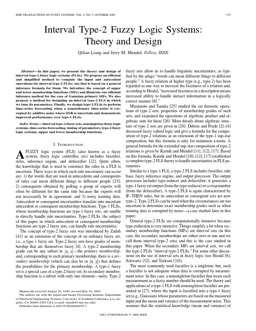
IEEE TRANSACTIONS ON FUZZY SYSTEMS, VOL. 8, NO. 5, OCTOBER 2000535Interval Type-2 Fuzzy Logic Systems: Theory and DesignQilian Liang and Jerry M. Mendel, Fellow, IEEEAbstract—In this paper, we present the theory and design of interval type-2 fuzzy logic systems (FLSs). We propose an efficient and simplified method to compute the input and antecedent operations for interval type-2 FLSs; one that is based on a general inference formula for them. We introduce the concept of upper and lower membership functions (MFs) and illustrate our efficient inference method for the case of Gaussian primary MFs. We also propose a method for designing an interval type-2 FLS in which we tune its parameters. Finally, we design type-2 FLSs to perform time-series forecasting when a nonstationary time-series is corrupted by additive noise where SNR is uncertain and demonstrate improved performance over type-1 FLSs. Index Terms—Interval type-2 fuzzy sets, nonsingleton fuzzy logic systems, time-series forecasting, tuning of parameters, type-2 fuzzy logic systems, upper and lower membership functions.I. INTRODUCTION FUZZY logic system (FLS) (also known as a fuzzy system, fuzzy logic controller, etc) includes fuzzifier, rules, inference engine, and defuzzifier [22]. Quite often, the knowledge that is used to construct the rules in a FLS is uncertain. Three ways in which such rule uncertainty can occur are: 1) the words that are used in antecedents and consequents of rules can mean different things to different people [23]; 2) consequents obtained by polling a group of experts will often be different for the same rule because the experts will not necessarily be in agreement; and 3) noisy training data. Antecedent or consequent uncertainties translate into uncertain antecedent or consequent membership functions. Type-1 FLSs, whose membership functions are type-1 fuzzy sets, are unable to directly handle rule uncertainties. Type-2 FLSs, the subject of this paper, in which antecedent or consequent membership functions are type-2 fuzzy sets, can handle rule uncertainties. The concept of type-2 fuzzy sets was introduced by Zadeh [41] as an extension of the concept of an ordinary fuzzy set, i.e., a type-1 fuzzy set. Type-2 fuzzy sets have grades of membership that are themselves fuzzy [4]. A type-2 membership —the primary membership; grade can be any subset in and, corresponding to each primary membership, there is a sec) that defines ondary membership (which can also be in the possibilities for the primary membership. A type-1 fuzzy set is a special case of a type-2 fuzzy set; its secondary membership function is a subset with only one element—unity. Type-2AManuscript received August 20, 1999; revised May 30, 2000. The authors are with the Signal and Image Processing Institute, Department of Electrical Engineering Systems, University of Southern California, Los Angeles, CA 90089-2564 USA (e-mail: mendel@). Publisher Item Identifier S 1063-6706(00)08455-1.fuzzy sets allow us to handle linguistic uncertainties, as typified by the adage “words can mean different things to different people.” A fuzzy relation of higher type (e.g., type-2) has been regarded as one way to increase the fuzziness of a relation and, according to Hisdal, “increased fuzziness in a description means increased ability to handle inexact information in a logically correct manner [6].” Mizumoto and Tanaka [25] studied the set theoretic operations of type-2 sets, properties of membership grades of such sets, and examined the operations of algebraic product and algebraic sum for them [26]. More details about algebraic structure of type-2 sets are given in [28]. Dubois and Prade [2]–[4] discussed fuzzy valued logic and give a formula for the composition of type-2 relations as an extension of the type-1 sup-star composition, but this formula is only for minimum -norm. A general formula for the extended sup-star composition of type-2 relations is given by Karnik and Mendel [11], [12], [17]. Based on this formula, Karnik and Mendel [10]–[12], [17] established a complete type-2 FLS theory to handle uncertainties in FLS parameters. Similar to a type-1 FLS, a type-2 FLS includes fuzzifier, rule base, fuzzy inference engine, and output processor. The output processor includes type-reducer and defuzzifier; it generates a type-1 fuzzy set output (from the type-reducer) or a crisp number (from the defuzzifier). A type-2 FLS is again characterized by IF–THEN rules, but its antecedent or consequent sets are now type-2. Type-2 FLSs can be used when the circumstances are too uncertain to determine exact membership grades such as when training data is corrupted by noise—a case studied later in this paper. General type-2 FLSs are computationally intensive because type-reduction is very intensive. Things simplify a lot when secondary membership functions (MFs) are interval sets (in this case, the secondary memberships are either zero or one and we call them interval type-2 sets) and this is the case studied in this paper. When the secondary MFs are interval sets, we call the type-2 FLSs “interval type-2 FLSs.” For some other discussions on the use of interval sets in fuzzy logic (see Hisdal [6], Schwartz [32], and Turksen [34]). The most commonly used fuzzifier is a singleton; but, such a fuzzifier is not adequate when data is corrupted by measurement noise. In this case, a nonsingleton fuzzifier that treats each measurement as a fuzzy number should be used. The theory and applications of a type-1 FLS with nonsingleton fuzzifier are presented in [27], where the input is fuzzified into a type-1 fuzzy set (e.g., Gaussian) whose parameters are based on the measured input and the mean and variance of the measurement noise. This assumes that the statistical knowledge (mean and variance) of1063–6706/00$10.00 © 2000 IEEE536IEEE TRANSACTIONS ON FUZZY SYSTEMS, VOL. 8, NO. 5, OCTOBER 2000the noise is given or can be estimated; but, in many cases, these values are not known ahead of time and can not be estimated from the data. Instead, we only have some linguistic knowledge about the noise, such as very noisy, moderately noisy, or approximately no noise. In this case, we cannot fuzzify the crisp input as a type-1 fuzzy set, because type-1 MFs cannot fully represent the uncertainty associated with this linguistic knowledge. We believe that in this important case, the input should be fuzzified into a type-2 fuzzy set for use in a nonsingleton type-2 FLS. This case is also studied in this paper. In this paper, we also provide a design method for an interval type-2 FLS, where IF–THEN fuzzy rules are obtained from given input–output (I/O) data. Two primary design tasks are structure identification and parameter adjustment [7]. The former determines input/output (I/O) space partition, antecedent and consequent variables, the number of IF–THEN rules (which are determined by the I/O space partition), and the number and initial locations of membership functions. The latter identifies a feasible set of parameters under the given structure. In this paper, we focus on parameter adjustments in an interval type-2 FLS. Tuning the parameters of a type-1 FLS is possible because can be expressed as a closed-form mathematical its output formula. Optimization methods for doing this have been extensively studied (for example, [7], [19], [22], [24], and [36]). Unfortunately, the output of a type-2 FLS cannot be represented by a closed-form mathematical formula; hence, there is an additional level of complexity associated with tuning its parameters. To date, type-2 sets and FLSs have been used in decision making [1], [40], solving fuzzy relation equations [35], survey processing, [12], [13], time-series forecasting [12], [14], function approximation [12], time-varying channel equalization [17], control of mobile robots [39], and preprocessing of data [9]. In the sequel, results for a general type-2 nonsingleton fuzzy logic system (NSFLS) are given in Section II; meet and join operations for interval sets are given in Section III; upper and lower membership functions that characterize a type-2 MF are introduced in Section IV; an efficient and simplified method to compute the input and antecedent operations for interval type-2 FLSs is given in Section V; type-reduction and defuzzification for an interval type-2 FLS are reviewed in Section VI; a method for designing an interval type-2 FLS is given in Section VII; an application of our design method is given in Section VIII for time-series forecasting of a nonstationary time-series that is corrupted by additive noise whose SNR is uncertain; and, finally, the conclusions and topics for future research are given in Section IX. denotes In this paper, denotes a type-1 fuzzy set; the membership grade of in the type-1 fuzzy set ; dedenotes the membership grade notes a type-2 fuzzy set; , of in the type-2 fuzzy set , i.e., ; denotes meet operation; and, denotes join operation. Meet and join are defined and explained in great detail in [10]–[12], [15]. II. TYPE-2 FLSS: GENERAL RESULTS In a type-2 FLS with a rule base of rules in which each rule has antecedents, let the th rule be denoted by , where : IF is , is , , and is , THEN is . Themembership function of a fired rule can be expressed by the following extended sup-star composition [12], [17]: (1) where is a -dimensional Cartesian product space, , is the measurement domain of input ); and is given by,((2) Additionally (3) Substituting (3) and (2) into (1), the latter becomes(4) Let (5) then(6) rules in the FLS fire, where Suppose that any of the ; then, the output fuzzy set, for a type-2 FLS is (7) For later use, we define (8) and (9) so that (6) can be re-expressed as (10) General type-2 FLSs are computationally intensive. Things simplify a lot when secondary MFs are interval sets, in which case secondary memberships are either zero or one and, as we demonstrate below, such simplifications make the use of type-2 FLSs practical. III. MEET AND JOIN FOR INTERVAL SETS The meet and join operations, which are needed in (5)–(10), can be greatly simplified for interval type-1 sets. Theorem 1 (Meet of Interval Sets Under Minimum or Product -Norms): and be two interval a) Let type-1 sets (often called interval sets) with domainsLIANG AND MENDEL: INTERVAL TYPE-2 FUZZY LOGIC SYSTEMS537( ), and ( ), respectively. The meet between and , ( ), under minimum or product -norms (i.e., ) is given by (11) . where b) The meet under minimum or product -norms of in, , having domains terval type-1 sets , , , respectively, where is an interval set with domain , . The proof of Theorem 1a), based on minimum or product operations between two interval sets, is given in [18] and [32]. The extension to part b) (via mathematical induction) is so straightforward, we leave it to the reader. Theorem 2 (Join of Interval Sets): a) Let and be as defined in part (a) of Theorem 1. The join ( ), is given by between and , (12) . where ( ) be as defined in Theorem 1(b). b) Let Then the join of these interval type-1 sets is an interval , . set with domain The proof of Theorem 2(a), based on maximum operation between two interval sets, is given in [18], [12], and [32]. The extension to part (b) (via mathematical induction) is also so straightforward we leave it to the reader. In this paper, we always assume that the operation is the maximum operation. Observe from Theorems 1 and 2, that meet and join operations of interval sets are determined just by the two end-points of each interval set. In a type-2 FLS, the two end-points are associated with two type-1 MFs that we refer to as upper and lower MFs. IV. UPPER AND LOWER MFS FOR TYPE-2 FLSS For convenience in defining the upper and lower MFs of a type-2 MF, we first give the definition of footprint of uncertainty of a type-2 MF. Definition 1 (Footprint of Uncertainty of a Type-2 MF): Uncertainty in the primary membership grades of a type-2 MF consists of a bounded region that we call the footprint of uncertainty of a type-2 MF (e.g., see Fig. 1). It is the union of all primary membership grades. Definition 2 (Upper and Lower MFs): An upper MF and a lower MF are two type-1 MFs that are bounds for the footprint of uncertainty of an interval type-2 MF. The upper MF is a subset that has the maximum membership grade of the footprint of uncertainty; and the lower MF is a subset that has the minimum membership grade of the footprint of uncertainty.Fig. 1. The type-2 MFs for (a) Example 1 and (b) Example 2. The thick solid lines denote upper MFs and the thick dashed lines denote lower MFs. The shaded regions are the footprints of uncertainty for interval secondaries. In (a), the centers of Gaussian MFs vary from 4.5–5.5; in (b), the center of the Gaussian MFs is 5 and the variance varies from 1.0–2.0.We use an overbar (underbar) to denote the upper (lower) MF. are For example, the upper and lower MFs of and , respectively, so that (13)Similarly, we will representandas (14) (15)538IEEE TRANSACTIONS ON FUZZY SYSTEMS, VOL. 8, NO. 5, OCTOBER 2000Example 1: Gaussian Primary MF with Uncertain Mean: Consider the case of a Gaussian primary MF having a and an uncertain mean that takes fixed standard deviation , i.e., on values inExample 2: Gaussian Primary MF with Uncertain Standard Deviation: Consider the case of a Gaussian primary MF having a fixed mean and an uncertain standard deviation that takes , i.e., on values in(16) where ; number of antecedents; ; and, number of rules. is [see Fig. 1(a)] The upper MF where ; number of antecedents; ; number of rules. is [see Fig. 1(b)] The upper MF(19)(20) (17) and the lower MF is [see Fig. 1(b)] (21) where, for example Note that the upper and lower membership functions are simpler for Example 2 than for Example 1. These examples illustrate how to define and so it is clear how to define these membership functions for other situations (e.g., triangular, trapezoidal, bell MFs). V. INTERVAL TYPE-2 FLSS (18) Our major result for interval type-2 FLSs is given in: Theorem 3: In an interval type-2 nonsingleton FLS with type-2 fuzzification and meet under minimum or product -norm: 1) the result of the input and antecedent operations, in (9), is an interval type-1 set, i.e., , whereThe lower MFis [see Fig. 1(a)]From this example, we see that sometimes an upper (or a lower) MF cannot be represented by one mathematical function over its entire domain. It may consist of several branches each defined over a different segment of the entire domain. When the input is located in one domain-segment, we call its corresponding MF branch an active branch, e.g., in Example 1, , the active branch for when is . When an upper (or lower) MF is represented in different segments, its left-hand and right-hand derivatives at the segment for ] may not end point [e.g., be equal, so the upper (or lower) MF may not be differentiable over the entire domain; however, it is piecewise differentiable, i.e., each branch is differentiable over its segment domain. This fact will be used by us when we tune the parameters of a type-2 FLS. Some upper and lower MFs can be represented by one function and are differentiable over their entire domain as we demonstrate in the following example.(22) and(23) the supremum is attained when each term in brackets attains its fired output consequent set in supremum; 2) the rule (10) is (24) and are the lower and upper membership where ; and 3) the output fuzzy set in (7) is grades of (25), as shown at the bottom of the page.(25)LIANG AND MENDEL: INTERVAL TYPE-2 FUZZY LOGIC SYSTEMS539A. Proof of Theorem 3 1) Applying Theorem 1(a) to (5) for an interval type-2 FLS with type-2 fuzzifier and using (14) and (15), we findThe suprema in (31) and (32) are, overall, in . By the monotonicity property of a -norm [42], [27], the supremum is attained when each term in brackets attains its supremum. 2) Based on (9), (31), (32), and Theorem 2(a), we evaluate (10) as(26) . So, the meet between an input type-2 where set and an antecedent type-2 set just involves the -norm operation between the points in two upper or lower MFs. are The upper and lower MFs of (27) (28) The meet operations in (8) are in a -dimensional Cartesian product space so the meet operation is over all , . Based on Theorem 1(b), points , we know that the upper membership grades of (a type-1 MF) are obtained from the -norm of ; hence, from (27), we find membership grades in ( 3) Because straightforward to obtain 2(b). The result is (25).(33) ) are interval sets, it is in (7) using TheoremIn evaluating (22) and (23), the supremum is attained when each term in brackets attains its supremum; so, in the inference of a type-2 FLS, we will examine (34) (35) where re-expressed as , and is a -norm; then, and can be(29) (36) (a type-1 MF), are The lower membership grades ; hence, the -norm of the membership grades in from (28) we find (37) where denotes -norm. We illustrate (36) and (37) below in Section V-C. B. Corollaries to Theorem 3 (30) The join operation in (9) is over all points in . Based on Theorem 2, we know that the right-most point of the ) interval sets is the maximum value join of ( of all the right-most points in the interval sets; so, the right-most point of comes from the maximum value (the right-most point of interval set (supremum) of for each value of ); hence, from (29) we find When the input is fuzzified to a type-1 fuzzy set so that ( ), the upper and lower MFs of merge into one MF in which case Theorem 3 simplifies to the following. Corollary 1: In an interval type-2 FLS with nonsingleton type-1 fuzzification and meet under minimum or product -norm, and in (22) and (23) simplify to(38) (31) Similarly, the left-most point maximum value (supremum) of we find of comes from the ; hence, from (30) and(39) ( ) is the type-1 fuzzified input. where When a singleton fuzzifier is used, the upper and lower MFs merge into one crisp value, namely one, in which of case Theorem 3 simplifies further to the following.(32)540IEEE TRANSACTIONS ON FUZZY SYSTEMS, VOL. 8, NO. 5, OCTOBER 2000Fig. 2. Type-2 FLS: input and antecedent operations. (a) Singleton fuzzification with minimum t-norm; (b) singleton fuzzification with product t-norm; (c) NS type-1 fuzzification with minimum t-norm; (d) NS type-1 fuzzification with product t-norm; (e) NS type-2 fuzzification with minimum t-norm; and (f) NS type-2 fuzzification with product t-norm. The dark shaded regions depict the meet between input and antecedent [computed using Theorem 1(a)].Corollary 2: In an interval type-2 FLS with singleton fuzzification and meet under minimum or product -norm and in (22) and (23) simplify to (40) and (41) ) denotes the location of the singleton. where ( The proofs of these corollaries are so simple, we leave them for the reader.C. Illustrative Examples Example 3—Pictorial Representation of Input and Antecedent Operations: In Fig. 2, we plot the results of input and antecedent operations with singleton, type-1 nonsingleton, and type-2 nonsingleton fuzzifications. The number of antecedents is . In all cases, the firing stength is an interval type-1 , where and . For set, denotes the singleton fuzzification [Fig. 2(a) and (b)], and , namely ; firing strength between input denotes the firing strength between input and , andLIANG AND MENDEL: INTERVAL TYPE-2 FUZZY LOGIC SYSTEMS541xTABLE I FOR EXAMPLE 4xFORTABLE II EXAMPLE 4 BASED ON PRODUCT t-NORMnamely , , as established by Corollary 2. For nonsingleton type-1 fuzzification [Fig. 2(c) and (d)], denotes the supremum of the firing strength between the -norm of membership functions and ; and denotes the supremum of the firing strength between the -norm of and , , as established membership functions by Corollary 1. For nonsingleton type-2 fuzzification [Fig. 2(e) denotes the supremum of the firing strength and (f)], and between the -norm of upper membership functions ; and, denotes the supremum of the firing strength and between the -norm of lower membership functions , , as established by Theorem 3. The main thing to observe from these figures is that regardless of singleton or nonsingleton fuzzification and minimum or product -norm, the result of input and antecedent operations is an interval type-1 set that is determined by its left-most point and right-most point . Example 4—Input is a Gaussian Primary MF with Uncertain Standard Deviation and Antecedents are Gaussian Primary MFs with Uncertain Means: In this example, we compute and when a Gaussian primary MF with an uncertain standard deviation (as in Example 2) is used as input fuzzy sets and Gaussian primary MFs with uncertain means (as in Example 1) are used as antecedent MFs. This case is important to our time-series forecasting application in Section VIII. In this caseby , and lowing form:by. The th antecedent MF has the fol-(43) and its upper and lower MFs and are obtainedby , from (17) and (18), respectively, by replacing by and by . Observe that there are six pa, rameters that determine these two type-2 Gaussian MFs: , , , , and . In this example, as in [27], we assume that (44) and our objective is to evaluate (34) and (35). Equation (44) means that uncertainty in each input set is always no more than the uncertainty in the antecedent. at which the supremum of (34) We denote the value of and the value of at which the supremum of occurs as . The results for and of this (35) occurs as example are carried out in Appendix A, and are summarized in Tables I–III. From these results, it is straightforward to compute and using (34) and (35), i.e., (45) (46)(42) and and its upper and lower MFs from (20) and (21), respectively, by replacing are obtained by , When the input is fuzzified to a type-1 Gaussian MF, then , and we can easily obtain and based on Tables I–III. When a singleton fuzzifier is used, the542IEEE TRANSACTIONS ON FUZZY SYSTEMS, VOL. 8, NO. 5, OCTOBER 2000xFORTABLE III EXAMPLE 4 BASED ON MINIMUM t-NORMresults in Tables I–III simplify even further since . VI. TYPE REDUCTION AND DEFUZZIFICATION . After fuzzification, A type-2 FLS is a mapping fuzzy inference, type-reduction, and defuzzification, we obtain a crisp output. For an interval type-2 FLS, this crisp output is the center of the type-reduced set. Based on Theorem 3 and Corollaries 1 and 2, we know that for an interval type-2 FLS, regardless of singleton or nonsingleton fuzzification and minimum or product -norm, the result of input and antecedent operations (firing strength) is an interval type-1 set, which is determined by and (e.g., see Fig. 2). its left-most and right-most points of rule can be obThe fired output consequent set tained from the fired interval strength using (24) or Corollaries 1 or 2 and (24). Then the fired combined output consequent set can be computed using (25). Type-reduction was proposed by Karnik and Mendel [11], [12], [17]. It is an “extended version” [using the extension principle [41] of type-1 defuzzification methods and is called typereduction because this operation takes us from the type-2 output sets of the FLS to a type-1 set that is called the “type-reduced set.” This set may then be defuzzified to obtain a single crisp number; however, in many applications, the type reduced set may be more important than a single crisp number since it conveys a measure of uncertainties that have flown through the type-2 FLS. There exist many kinds of type-reduction, such as centroid, center-of-sets, height, and modified height, the details of which are given in [11], [12], and [17]. In this paper, for illustrative purposes, we focus on center-of-sets type-reduction, which can be expressed ascentroid of the type-2 interval conse(the centroid of a type-2 quent set fuzzy set is described in [11], [16], and [12]); . Observe, that each set on the right-hand side (RHS) of (47) is an interval type-1 set, hence, is also an interval type-1 set. So, to find , we just need to compute the two end-points of this interval. Unfortunately, no closed-form . formula is available for , can be represented as For any value and(48)and the minimum value of is the maximum value of is . From (48), we see that is a monotonic increasing function with respect to ; so is associated only with and, similarly, is associated only with . In the center of sets (COS)-typereduction method, Karnik and Mendel [12], [17] have shown , , and depend only on a that the two end points of mixture of or values, since . In this case, and can each be represented as a fuzzy basis function (FBF) expansion, i.e.,(49)(47)where [eitherdenotes the firing strength membership grade or ] contributing to the left-most point and is the FBF. Similarlywhere interval set determined by two end points and ; ; (50)LIANG AND MENDEL: INTERVAL TYPE-2 FUZZY LOGIC SYSTEMS543denotes the firing strength membership grade (either ) contributing to the right-most point and is another FBF. Note that whereas a type-1 FLS is characterized by a single FBF expansion [22], [37], an interval type-2 FLS is characterized by two FBF expansions. A general type-2 FLS is characterized by a huge number of FBF expansions [12], [17]; hence, we have demonstrated that by choosing secondary membership functions to be interval sets, the complexity of a general type-2 FLS is vastly reduced. In order to compute and , we need to compute and . This can be done using the exact computational procedure given in [12], [16], and [17]. Here, we briefly provide the computation procedure for . Without loss of generality, assume the s are arranged in . ascending order, i.e., 1) Compute for in (50) by initially setting , where and have been previously . . andwhere orVII. DESIGNING INTERVAL TYPE-2 FLSS BASED ON TUNING , and Given an input–output training pair , we wish to design an interval type-2 FLS with output (53) so that the error function (54) is minimized. Based on the analysis in Section VI, we know that (the only the upper and lower MFs and the two endpoints of . So we want to center of the consequent set) determine tune the upper and lower MFs and the consequent parameters . Since an interval type-2 FLS can be characterized by two FBF expansions that generate the points and , respectively, we can focus on tuning the parameters of just these two type-1 FLSs. input–output training samples , Given ), we wish to update the design parameters ( so that (54) is minimized for training epochs (updating the parameters using all the training samples one time is called “one epoch”). A general method for doing this is as follows. 1) Initialize all the parameters including the parameters in antecedent and consequent MFs and input sets. . 2) Set the counter of training epoch . 3) Set the counter of training data sample input to the type-2 FLS, and compute the 4) Apply total firing degree for each rule, i.e., compute and ( ) using Theorem 3. 5) Compute and , as described in Section VI (which rules; but, they are then leads to a reordering of the renumbered 1, 2, , ). This will establish and , so that and can be expressed ascomputed using (22) and (23) and let ) such that 2) Find ( for 3) Compute in (50) withfor and let . , then go to Step 5). If , then stop and 4) If . set and return to Step 2). 5) Set equal to This four-step computation procedure [Step 1) is an initialization step] has been proven to converge to the exact solution iterations [12]. Observe that in this procein no more than , , and dure, the number is very important. For , ; so can be represented as for (51) The procedure for computing is very similar. Just replace by and, in Step 2), find ( ) such that and, in step 3, let for , and for . Then can be represented as (52)(55)(56) is an interval set, we defuzzify it using the avBecause erage of and ; hence, the defuzzified output of an interval type-2 FLS is , which is the defuzzified 6) Compute output of the type-2 FLS. and on 7) Determine the explicit dependence of and obtained in membership functions (because Step 5) may have changed from one iteration to the next, the dependence of and on MFs may also have changed). To do this, first determine the dependence of and on membership functions, using (34)–(37), is determined by , , , i.e.,(53) , where is the deA perfect FLS should have sired output but, generally, there exist errors between the desired output and actual output. We, therefore, need a design procedure for tuning the parameters of the FLS in order to minimize such errors.。
optimization method

• The eventual intention behind using operations research is to elicit a best possible solution to a problem mathematically, which improves or optimizes the performance of the system.
14
1. Introduction
Historical development • Albert William Tucker (1905-1995) (Necessary and sufficient conditions for the optimal solution of programming problems, nonlinear programming, game theory: his PhD student was John Nash) • Von Neumann (1903-1957) (game theory)
Computers and Structures International Journal for Numerical Methods in Engineering Structural Optimization Journal of Optimization Theory and Applications Computers and Operations Research Operations Research and Management Science
9
1. Introduction
• Operations research (in the UK) or operational research (OR) (in the US) or yöneylem araştırması (in Turkish) is an interdisciplinary branch of mathematics which uses methods like:
optimization_method

optimization_methodOptimization methods are the use of mathematical techniques to find the most efficient solutions to a given problem. They can be used to improve efficiency, identify designs, or develop strategies for decision-making. Examples of optimization methods include linear programming, nonlinear programming, integer programming, dynamic programming, simulated annealing, genetic algorithms, and fuzzy logic. These methods can be used to solve a variety of problems, such as optimization of a manufacturing process or a transportation network. Optimization methods are also used to maximize profit, minimize cost, and optimize utilization of resources.Linear programming is a type of optimization method that is used to maximize or minimize a linear objective function such as profit or cost. It involves making decisions about setting values for the variables in a system to optimize the objective function. The objective function is then used to determine the best combination of variables that will lead to the desired result.Nonlinear programming is another type of optimization method. It is used to find solutions to problems that involve relationships between variables that are not linear. Itinvolves solving equations and inequalities that represent the relationships between variables and then using an algorithm to find the optimal solution for the problem.Integer programming is an optimization method used to solve problems with integer values as variables. It is used to solve problems such as scheduling, resource allocation, and network design. It involves setting integer values for the variables and then using an algorithm to calculate the optimal solution. Dynamic programming is an optimization method used for decision problems with many states or decisions over time. It involves breaking down a complex problem into simplersub-problems, and then determining the optimal solution for the entire problem by solving the individual sub-problems.Simulated annealing is an optimization method used to find an optimal solution in problems that have a large number of possible solutions. It uses a process of trial and error to find the best solution. It is often used in optimization problems that can not be solved using traditional optimization methods. Genetic algorithms are optimization methods that use the principles of evolutionary biology to solve difficult problems. In this method, a population of solutions to a problem is evaluated and those solutions that are most successful areselected for further use. These new solutions are then used to replace the old generation of solutions and the process is repeated until an optimal solution is found.Fuzzy logic is a type of optimization method that is used to solve problems with uncertain or incomplete information. It involves assigning values to data points and then using heuristics and fuzzy logic to make decisions about the data. Fuzzy logic is often used to automate decision-making processes or to solve problems that cannot be solved with traditional methods.。
Optimization-Overview优化设计
– What are the “available means”?
• Design constraints, requirements
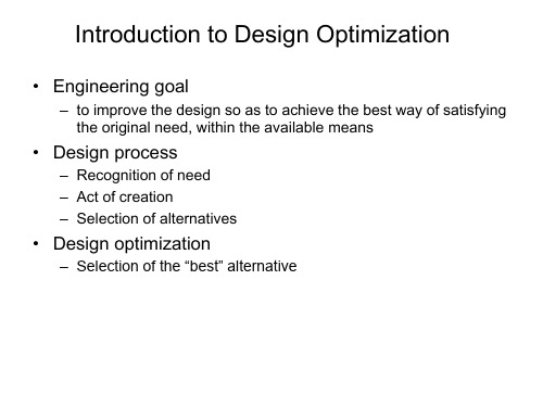
Introduction to Design Optimization
• Design optimization definitions
– The selection of a set of variables to describe the design alternatives. – The selection of an objective (criterion), expressed in terms of the design variables, which we seek to minimize or maximize. – The determination of a set of constraints, expressed in terms of the design variables, which must be satisfied by any acceptable design. – The determination of a set of values for the design variables, which minimize (or maximize) the objective, while satisfying all the constraints.
Introduction to Design Optimization
• Engineering goal
– to improve the design so as to achieve the best way of satisfying the original need, within the available means
Engineering Design and Optimization
Engineering Design and OptimizationEngineering design and optimization is a critical process in the development of new products, systems, and processes. It involves the application of scientific and mathematical principles to create efficient and effective solutions to complex problems. The goal of engineering design and optimization is to improve the performance, reliability, and cost-effectiveness of products and systems, while also minimizing their environmental impact. This process requires a deep understanding of the underlying principles of physics, mathematics, and materials science, as well as the ability to think creatively and innovatively. One of the key challenges in engineering design and optimization is the need to balance competing objectives. For example, when designing a new product, engineers must consider factors such as performance, cost, reliability, and manufacturability. These objectives are often conflicting, and it can be difficult to find a solution that optimizes all of them simultaneously. This requires careful analysis and trade-off decisions, as well as the use of advanced optimization techniques tofind the best possible solution. Another challenge in engineering design and optimization is the need to account for uncertainty. In many engineering problems, there are uncertainties in factors such as material properties, operating conditions, and external loads. These uncertainties can have a significant impact on the performance and reliability of the final design. Engineers must therefore use probabilistic methods and robust design techniques to account for these uncertainties and ensure that the final design is resilient to variations in operating conditions. In recent years, there has been a growing emphasis on sustainability in engineering design and optimization. This includes the need to minimize the environmental impact of products and systems, as well as to optimize their energy efficiency and use of natural resources. This requires a holistic approach that considers the entire life cycle of a product, from raw material extraction to end-of-life disposal. Engineers must therefore consider factors such as material selection, energy efficiency, and recyclability when optimizing the design of new products and systems. Advances in computer-aided design (CAD) and simulation tools have revolutionized the field of engineering design and optimization. These tools allow engineers to create detailed virtual models ofproducts and systems, and to simulate their performance under various operating conditions. This enables engineers to explore a wide range of design options andto quickly evaluate their performance, cost, and reliability. As a result, the design process has become more iterative and collaborative, with engineers able to explore a larger design space and to quickly identify the best possible solutions. In conclusion, engineering design and optimization is a complex and challenging process that requires a deep understanding of scientific and mathematical principles, as well as the ability to balance competing objectives and account for uncertainty. It also requires a growing emphasis on sustainability and environmental impact, as well as the use of advanced CAD and simulation tools. By addressing these challenges, engineers can create innovative and effectivesolutions to the complex problems of the modern world.。
风力越野车的优化设计方案

风力越野车的优化设计方案引言风力越野车是一种利用风能驱动的无污染的交通工具,适用于各种地形和路况。
为了提高风力越野车的性能和效率,本文将探讨该车型的优化设计方案。
优化方案一:轻量化设计1.使用高强度轻质材料,如碳纤维复合材料和铝合金等,来替代传统的钢材。
2.精简车身结构,去除不必要的部件和附件。
3.采用轻量化设计的底盘和悬挂系统,减少车辆自重,提高悬挂系统的负荷能力。
优化方案二:动力系统改进1.采用高效的风能转换系统,提高风能的转换效率。
2.使用先进的电动机和电池技术,提高驱动系统的效率和续航能力。
3.结合太阳能充电系统,增加能源的可持续利用性。
优化方案三:悬挂系统升级1.采用可调节的悬挂系统,根据不同路况和行驶速度,调整车辆的悬挂高度和刚度,提高车辆行驶的舒适性和稳定性。
2.使用增压气囊悬挂系统,提供更好的减震和支撑功能。
3.引入主动悬挂控制技术,实时监测车辆状态和路面情况,根据预设参数进行主动悬挂调整。
优化方案四:空气动力学改进1.优化车身外形设计,减小空气阻力,提高行驶效率。
2.添加风洞测试装置,对车辆进行空气动力学性能测试和优化。
3.使用尾翼和导流板等空气动力学附件,减少气动阻力,提高车辆稳定性。
优化方案五:智能化系统引入1.引入智能驾驶辅助系统,包括自动驾驶、自动泊车和自动避障等功能,提高行车安全性。
2.使用智能导航系统,优化路线规划和导航功能,提高行驶效率。
3.结合互联网技术,实现远程控制和车辆信息交互,提供更便捷的使用体验。
结论通过轻量化设计、动力系统改进、悬挂系统升级、空气动力学改进和智能化系统引入等优化方案,可以提高风力越野车的性能和效率。
这些优化措施将使风力越野车更加环保、高效、舒适和安全,为人们提供一种可持续的出行方式。
参考文献•Smith, J. L., & Anderson, A. (2009). Optimization methods for engineering design. Courier Corporation.•Zhang, Q., & Cheng, G. H. (2015). Design optimization for engineering systems. CRC Press.•Chen, G., Qi, X. F., & Liu, J. G. (2018). Structural optimization design of racing car under vibration and noise constraints. Shock and Vibration, 2018.。
《生产运营管理英文》课件

01
Introduction
Ensuring effective production processes
Production and operation management safeguards that production processes are carried out efficiently, minimizing waste and maximizing output
The production process should pursue high efficiency, reduce production costs, and improve output efficiency.
Flexibility
The production process should have flexibility to cope with various changes and uncertainties in the production process.
Production and operation strategy is an important component of enterprise strategy, which involves multiple aspects of the enterprise's production system, operation system, supply chain system, etc., and has a crucial impact on the development of the enterprperation management involves the planning, organization, control, and coordination of production and operations processes to achieve desired results
专业英语课程论文-油气储运工程TechnicalEnglishforOilandGas

T echnical English for Oil and GasStorage and T ransportation Engineering Since September this year, we have had a new course called Technical English for oil and gas storage and transportation engineering. Professor Liu is the teacher of this course and she is very well to us. In the teaching of Professor Liu, I get much knowledge and I fell very happy.Now,let me write somethings about my profession with some personnal ideals.Extensive Reading①The title of the first paper I viewed is “Fluid and Hydraulic System”.As far as I am concerned,this paper mainly describes two important contents which are fluid and hydraulic system.The former part of this paper gives an account of Fluid that is a substance which may flow.Its constituent particles may continuously change their positions relative to one another.Moreover,it offers no lasting resistance to the displacement,however great ,of one layer over another.This means that,if the fluid is at rest,no shear force(that is a force tangential to the surface on which it acts)can exist in it.Meanwhile,fluid may be classified as Newtonian or non- Newtonian.In Newtonian fluid there is a linear relation between the magnitude of applied shear stresses and the resulting rate of angulardeformation.In non- Newtonian fluid there is a nonlinear relation between the magnitude of applied shear stresses and the resulting rate of angular deformation.The after part of this paper is concerned with the hydraulic system. I think the ligament between the two sides is “Pascal’s law”. Because all hydraulic systems depend on Pascal’s law,named after Braise Pascal, who discovered the law. This law states that pressurized fluid within a closed container-such as cylinder or pipe-exerts equal force on all of the surfaces of the container. Moreover, in actual hydraulic systems, Pascal’s law defines the basis of the results which are obtained from the system.Thus,pump moves the liquid in the system. The intake of the pump is connected to a liquid source,usually called the tank or reservoir. Atmospheric pressure,pressing on the liquid in the reservior,forces the liquid into the pump.when the pump operates,it forces liquid from the tank into the discharge pipe at a suitable pressure.②The title of the second paper I viewed is “A Discussion on Modern Design Optimization”. In this paper,the author focuses on the theory underlying some of the mathematical methods employed by design optimization procedures.To begin with, this paper treats of the optimization techniques taking one with another. The integration of optimization techniqueshas the power to reduce design costs by shifting the burden from the engineer to the computer. Furthermore,the mathematical rigor of a properly implemented potimization tool can add confidence to the design process.Modern optimization methods perform shape optimizations on components generated within a choice of CAD packages. Ideally, there is seamless data exchange via direct memory transfer between the CAD and FEA applications without the need for file translation. Furthermore, if associativity between the CAD and FEA software exist, any changes made in the CAD geometry are immediately reflected in the FEA model.The second, this paper describe how the optimization problem arises. Consider a three-step process:(1)Generation of geometry of part or assembly in CAD;(2)Creation of FEA mode of part or assembly;(3)Evaluation of results of FEA models.Meanwhile,most optimization problems are made up of three basic components.(1) An objective function which we want to minimize (or maximize). For instance, in designing an automobile panel, we might want to minimize the stress in a particular region.(2) A set of design variables that affect the value of theobjective function. In the automobile panel design problem, the variables used define the geometry and material of the panel.(3) A set of constraints that allow the design variables to have values but exclude others. In the automobile panel design problem, we would probably want limit its weight.The last but not the least, there is no beauideal in the world. Modern design optimization has many benefits and drawbacks. The elimination or reduction of repetitive manual tasks has been the impetus behind many software applications. Automatic design optimization is one of the latest applications used to reduce man-hours at the expense of possibly increasing the computational effort. It is even possible that an automatic design optimization scheme may actually require less computational effort than a manual approach. This is because the mathematical rigor on which these schemes are based may be more efficient than a human-based solution. Of course, these schemes do not replace human intuition, which can occasionally significantly shorten the design cycle. That is, no variable combination of the design parameters is left unconsidered. Thus,designs obtained using design optimization software should be accurate to within the resolution of the overall method.Intensive ReadingOriginal textIndustrial RobotA robot is an automatically controlled, reprogrammable, multipurpose, manipulating machine with several reprogrammable axes, which may be either fixed in place or mobile for use in industrial automation applications.The key words are reprogrammable and multipurpose because most single-purpose machines do not meet these two requirements. The term “multipurpose”means that the robot can perform many different functions, depending on the program and tooling cureently in use.Over the past two decades, the robot has been introduced into industry to perform many monotonous and often unsafe operations. Because robot can perform certain basic tasks more quickly and accurately than humans, they are being increasingly used in various manufacturing industries.The typical structure of industrial robot consists of 4 major components: the manipulator, the end effector, the power supply and the control system.The manipulator is a mechanical unit that provide motions similar to those of a human arm. It often has a shoulder joint, an elbow and a wrist. It can rotate or slide, stretch out and withdraw inevery possible direction with certain flexibility.The basic mechanical configurations of the robot manipulator are categorized as cartesian, cylindrical, spherical and ariculated. A robot with a cartesian geometry can move its gripper to any position within the cube or rectangle defined as its working volume. Cylindrical coordinate robots can move the gripper within a volume that is described by a cylinder. The cylindrical coordinate robot is positioned in the work area by two linear movements in the X and Y directions and one angular rotation about the axis. Spherical arm geometry robots position the wrist through two rotation and one linear actuation. Articulated industrial robots have an irregular work envelope. This type of robot has two main variants,vertically articulated and horizontally articulated.The end effector attaches itself to the end of robot wrist, also called end-of-arm tooling. It is the device intended for performing the designed operations as a human as a human hand can. End effectors are generally custom-made to meet special handling requirements. Mechanical grippers are the most commonly used and are equipped with two or more fingers. The selection of an appropriate end effector for a specific application depends on such factors as the payload, environment, reliability, and cost.The power supply is the actuator for moving the robot arm,controlling the joints and operating the end effector. The basic types of power sources include electrical, pneumatic, and hydraulic. Each source of energy and each type of motor has its own characteristics, advantages and limitations. An ac-powered or dc-powered motor may be used depending on the systerm design and applications. These motors convert electrical energy into mechanical energy to power the robot. Most new robot use electrical power supply. Pneumatic actuators have been used for high speed, nonservo robots and are often used for powering tooling such as grippers. Hydraulic actuators have been used for heavier lift system, typically where accuracy was not also required.The control system is the communications and information-processing system that gives commands for the movements of the robot. It is the brain of the robot; it sends signals to the power source to move the robot arm to a specific position and to actuate the end effector. It is also the nerves of the robot ; it is reprogrammable to send out sequences of instructions for all movements and actions to be taken by the robot.An open-loop controller is the simplest form of the control system, which controls the robot only by following the predetermined step-by-step instructions. This system does not have a self-correcting capability. A close-loop control system uses feedbacksensors to produce signals that felect the current states of the controlled objects. By comparing those feedback signals with the values set by the programmer, the close-loop controller can conduct the robot to move to the precise position and assume the desired attitude, and the end effector can perform with very high accuracy as the close-loop control system can minimize the discrepancy between the controlled object and the predetermined references.Industrial robots vary widely in size, shape, number of axes, degrees of freedom, and design configuration. Each factor influences the dimensions of the robot’s working envelope or the volume of space within which it can move and perform its designated task. A broader classification of robots can been described as below.Fixed-and V ariable-Sequence Robots. The fixed-sequence robot(also called a pick-and place robot) is programmed for a specific sequence of operation. Its movements are from point to point, and the cycle is repeated continuously. The variable-sequence robot can be programmed for a specific sequence of operations but can be reprogrammed to perform another sequence of operation.Playback Robot. An operator leads or walks the playback robot and its end effector through the desired path. The robot memorizes and records the path and sequence of motions and can repeat them continually without any further action or guidance by the operator.Numerically Controlled Robot. The numerically controlled robot is programmed and operated much like a numerically controlled machine. The robot is servo-controlled by digital data, and its sequence of movements can be changed with relative ease.Intelligent Robot. The intelligent robot is capable of performing some of the functions and tasks carried out by human beings. It is equipped with a variety of sensors with visual and tactile capabilities.The robot is a very special type of production tool; as a result, the applications in which robots are used are quite broad. These applications can be grouped into three categories: material processing, material handing and assembly.In material processing, robot use tools to process the raw material. For example, the robot tools could include a drill and the robot would be able to perform drilling operations on raw material.Material handing consists of the loading, unloading, and transferring of workpieces in manufacturing facilities. These operations can be performed reliably and repeatedly with robots, thereby improving quality and reducing scrap losses.Assembly is another large application area for using robotics. An automatic assembly system can incorporate automatic testing, robot automation and mechanical handing for reducing labor costs,increaing output and eliminating manual handing concerns.What I have learned form the upper paper is listed as followNowadays, along with the fast pace of economic development, more and more Industrial robots have been presented in our living. Industrial robots have many merits and their applications are very abroad in the world.The former three paragraphs of the paper mainly introduce the short and the long of the industrial robots. W e generally realize the functions and use of them. W e know that robots have been used in various vocations. There is a word “reprogrammable”that attracts me in the second paragraph. In my opinion, the term “reprogrammable” implies two things: The robot operates according to a written program, and this program can be written to accommodate a variety of manufacturing tasks.From 4th to 10th paragraph, this paper mainly introduce the structures of robots. There are a large number of professional words which I list as follow.Elbo(肘) wrist(腕) shoulder joint(肩关节) Coordinate(坐标) volume(范围) cylindrical(圆柱的) spherical(球状的) open-loop(开环) close-loop(闭环) articulated(铰接的) cartesian(笛卡尔的) pneumatic(气动的) payload(有效载荷) feedback(反馈) nonservo(非伺服系统) end effector(终端操作机构)When I read the first sentence of the 4th paragraph, I wonde what is the mechanical unit. V ia some reference books, I know that the major of mechanism is the mechanical system. And the mechanical system is decomposed into mechanisms,which can be further decomposed ino mechanical components. In this sense, the mechanical components are the fundamental elements of machinery. On the whole, mechanical components Can be classified as universal and special components.From 11th to 15th paragraph, this paper mainly introduce the classification of robots. In the point, the classification is presented broad sense. as a matter of fact, there are a lot of categorys of the classification. What attracts me is the word “playback”. The original intention of “playback”is “repeatedly play”, but over here, it’s meaning is “示教”.The last four paragraphs mainly introduce several robot applications. At present there are two main types of robots, based on their use: general-purpose autonomous robots(通用机器人)and dedicated robots(专用机器人). Robots can be classified by their specificity of purpose. There are many application in our society nowadays. For example, in our school, they has three main applications: Robotic kits, V irtual tutors and teacher's assistants.Along with various techniques having emerged to develop the science of robotics and robots, One method shows itself that is evolutionary robotics, in which a number of differing robots are submitted to tests. Those which perform best are used as a model to create a subsequent "generation" of robots. Another method is developmental robotics, which tracks changes and development within a single in the areas of problem-solving and other functions.In a word, the prospect of robots is very bright.Appendix: all the papers in my discourse are extracted from the book named Technical English published in Peking University Press that borrowed from the library of my school.。
topology[1]
![topology[1]](https://img.taocdn.com/s3/m/ee0a60ff770bf78a65295437.png)
40
No design area (No material)
24
Result of Design Constraint
Influence of Design Domain
12 2 2 1.25 Design Domain 5
1.25
Non-design Domain
1.25
Design Domain
max u s f
design
T
5
Lagrangian
NE 1 NE T T L = ∑ d e K ed e − d e fe + λ ∑ ρ e Ae Le − W 2 e =1 e =1
Total Potential Energy Weight Constraint
new
Shape Design Find the best Ω
Material Design Find the best Dnew
15
Homogenization Design Method
• Shape and Topology Design of Structures is transferred to Material Distribution Design (Bendsoe and Kikuchi, 1988)
min
∑ρ A L
e =1 e e
e
Design Sensitivity
K
P1 P2
∂u ∂K ∂f =− u+ ∂Ae ∂Ae ∂Ae
∂u ∂σ e ∂ De Be ue = De Be e = ∂Ae ∂Ae ∂Ae ∂ ui u ∂u = i • i ∂Ae ui ∂Ae
Optimization Techniques in Algorithm Design
Optimization Techniques in AlgorithmDesignIn algorithm design, optimization techniques play a crucial role in improving the efficiency and effectiveness of algorithms. These techniques are the methods used to optimize the algorithm to achieve better performance in terms of speed, memory usage,or other relevant metrics.One common optimization technique in algorithm design is the use of data structures. By choosing the appropriate data structure for a specific problem, algorithms can be optimized to perform operations more efficiently. For example, using a hash table instead of a simple array can significantly reduce the time complexity of certain operations, such as searching or inserting elements.Another optimization technique is the use of dynamic programming, which involves breaking down a complex problem into smaller subproblems and solving them recursively. By storing the solutions to subproblems in a table and reusing them when needed, dynamic programming can improve the overall efficiency of algorithms, particularly for problems with overlapping subproblems.Furthermore, greedy algorithms are another optimization technique commonly used in algorithm design. Greedy algorithms make locally optimal choices at each step with the hope of finding a globally optimal solution. While greedy algorithms are not always guaranteed to find the optimal solution, they are often used in situations where finding the exact solution is less important than finding a solution that is close to optimal.In addition to data structures, dynamic programming, and greedy algorithms, there are many other optimization techniques that can be employed in algorithm design. These include divide and conquer, backtracking, branch and bound, and many more. Each technique has its own strengths and weaknesses, and the choice of which technique to use depends on the specific characteristics of the problem being solved.Overall, optimization techniques are essential in algorithm design to ensure that algorithms are efficient, effective, and capable of solving complex problems in a timely manner. By understanding and implementing these techniques, algorithm designers can create algorithms that outperform others and provide optimal solutions for a wide range of problems.。
文得根水利枢纽粘土心墙坝反滤层设计及优化
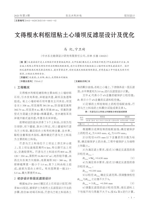
文得根水利枢纽粘土心墙坝反滤层设计及优化马纪,宁卫琦(中水东北勘测设计研究有限责任公司,吉林长春130021)[摘要]反滤层设计是土石坝设计的重要组成部分,文中依据《碾压式土石坝设计规范》中反滤层设计方法,结合施工现场土料场与坝体砂砾石的颗粒级配曲线,进行文得根水利枢纽粘土心墙砂砾石坝反滤层设计。
设计的反滤料除满足规范要求的保土、透水等要求外,同时还满足级配连续的要求,并考虑施工中可能发生的不利因素,以保证大坝的安全。
[关键词]反滤层;土石坝;粘土;文得根水利枢纽[中图分类号]TV641.2+[文献标识码]B[文章编号]1002—0624(2021)03—0001—021工程概况文得根水利枢纽建筑物主要由粘土心墙砂砾石坝、引水发电系统、岸坡溢洪道、副坝及鱼道等组成。
粘土心墙砂砾石坝布置在主河床处,坝顶全长1358m,坝顶高程381.50m,防浪墙顶高程382.70m,坝顶宽8m,最大坝高48m。
坝基防渗型式为混凝土防渗墙+帷幕灌浆。
泄水建筑采用岸坡开敞式溢洪道,布置在右岸岸坡。
前期初设阶段共详查了5个土料场,分别为包尔胡舒、坝下缓坡、取水口附近、坝上缓坡和巴彦乌兰土料场,最后综合土料有机物含量、含水率、黏粒含量等技术指标,最终确定巴彦乌兰土料场为主要的粘土料场。
巴彦乌兰土料场位于上坝址上游左岸山坡上,至上坝址直线距离约6km,有公路可达上坝址,交通较便利。
巴彦乌兰土料场长约800m,宽120~350m,面积约16.86×10⁴m2,地形较平缓,由西北向东南方向倾斜,地面高程352~380m。
表部耕植厚度一般小于1.0m,其下土料由粘土组成,底部为混合土碎石。
有用层厚度一般2.5~5.0m,最大厚度约8m。
2初步设计阶段反滤层设计根据SL274-2001《碾压式土石坝设计规范》附录B.0.5规定,被保护土为粘性土反滤层设计方法的步骤,结合B1砂砾石料场、巴彦乌兰粘土料场各土体的颗分曲线,在粘土心墙上、下游侧各设一层反滤层,水平厚度均为3.0m,进行反滤层设计计算。
优化英语怎么说
优化英语怎么说优化是采取一定措施使变得优异。
为了更加优秀而“去其糟粕,取其精华”;为了在某一方面更加出色而去其糟粕;为了在某方面更优秀而放弃其他不太重要的方面;使某人/某物变得更优秀的方法/技术等;在计算机算法领域,优化往往是指通过算法得到要求问题的更优解。
那么你知道优点用英语怎么说吗?下面来学习一下吧。
优化的英语说法1:optimization优化的英语说法2:majorization优化的相关短语:优化保护 Optimal Protection结构优化structural improvement ; Structure optimization ; Refined Frameworks ; optimum structure程序优化 program optimization ; Programming Optimization ; Process optimization ; program optimizing拓扑优化 topological optimization ; topology optimization ; Topological Opt ; optimization优化的 Optimized ; optimal ; Optimizing ; optimizations优化方法Optimization Methods ; optimal design method ; optimization优点的英语例句:1. The new systems have been optimised for running Microsoft Windows.已经对这些新系统进行了优化设置,以便运行微软视窗。
2. We should optimize the composition of the standing committees.优化人大会组成人员的结构.3. Optimize for responsiveness; accommodate latency.优化响应能力, 调节延迟时间.4. We should optimize our import mix and focus on bringing in advanced technology and key equipment.优化进口结构,着重引进先进技术和关键设备.5. In some specialized products, it is appropriate to optimize the user experience for experts.在某些产品中, 为专家优化用户体验是合适的.6. We are often asked whether consumer Web sites should be optimized for beginners or intermediates.我们常常被问到这样的问题:消费类网站究竟应该为新手而优化,还是应该为中间用户而优化?7. At last, an optimal example for a boring cutting tool is presented.最后, 给出了优化计算实例.8. The advantages of Perl's design make all this optimization work worth while.Perl在设计上的优势使得所有这些优化都很值得.9. And the constrained - dominance is applied constrained multi - objective optimization problems efficiently.对于约束多目标优化问题,算法采用带约束支配关系判别个体的优劣.10. Emerson optimizes PlantWeb engineering work processes by joining Intergraph's SmartPlant alliance program.加入Intergraph的SmartPlant联盟计划,艾默生优化了PlantWeb工程工作步骤.11. Objective : To optimize the basic water extraction process of andrographis paniculata extract.目的: 对碱水法生产穿心莲浸膏工艺进行优化.12. Need to design crossover operator rationally while optimizing ANN.优化网络需要合理设计交叉算子.13. Withdrawal of state - owned stock helps optimize share - h olding structure of listed company.国有股退出有利于上市公司股权结构的优化.14. The iteration of geo - metrical programming with constrained positive - negative term equations is used.结果表明:该法与其它优化方法比较,可降低问题的困难度.15. Optimize inventory management skills and operation way of working.优化存货管理能力以及工作方式.。
多学科设计优化方法比较
弹箭与制导学报
2005 年
X
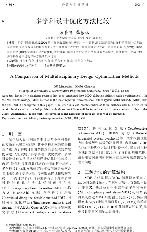
多学科设计优化方法比较*
谷良贤, 龚春林
( 西北工业大学航天学院, 陕西 西安 710072) [ 摘要] 多学科设计优 化( MDO) 是当前复杂系统 设计研究中一个 最新、最 活跃的领 域, 而多 学科设计 优方法 是多学科优化技术体系的研究核心。文中对具有代表性的三种多学科优化方法—多学科 可行法( MDF ) 、单学 科可行法( I DF ) 和协同 优化方法( CO) 进行比较, 阐述了各种方法的 结构体系及其特点, 并且通过 一个耦合的 多学科问题来说明三种方法的集成过程。 [关键词] 多学科优化; 多学科可行法; 单 学科可行法; 协同优化方法 [ 中图分类号] TJ 760. 2 [ 文献标识码] A
图 3 CO 计算原理图
3 实例分析
考虑 一 个包 含 三
个学科 W, Y, Z 的学科 优化问题[ 4] , 学科之间
的关 系和输 入输出 如
图 4 所示。
图 4 问题中, 目标 图 4 耦合的多学
函数和约束为:
科优化问题
Mi n F =
0.
04X
2 w
+
0. 96XY3 +
0.
15X
1 z
-
0. 26W21 + 0. 44W12 + 0. 57W33 -
X 收稿日期: 2004-07-08 基金项目: 本项目获得国家 863 计划基金资助( 2003AA721052) 、西北工业大学博士生创新基金资助。 作者简介: 谷良贤( 1957—) , 女, 河南沁阳人, 教授, 主要研究方向: 飞行器总体 设计, 多学科设计优化。
第 25 卷第 1 期
- 1、下载文档前请自行甄别文档内容的完整性,平台不提供额外的编辑、内容补充、找答案等附加服务。
- 2、"仅部分预览"的文档,不可在线预览部分如存在完整性等问题,可反馈申请退款(可完整预览的文档不适用该条件!)。
- 3、如文档侵犯您的权益,请联系客服反馈,我们会尽快为您处理(人工客服工作时间:9:00-18:30)。
*
To whom correspondence may be addressed: mark.gerstein@
1
Abstract A recent development in microarray construction entails the unbiased coverage, or tiling, of non-repetitive genomic DNA for the experimental identification of unannotated transcribed sequences and regulatory elements. A central issue in designing tiling arrays is one of sequence similarity, as significant experimental cross-hybridization can result from the incorporation of non-unique probe sequences. Many genomes contain thousands of repetitive elements that must also be identified and omitted from the array design. Due to the fragmentation introduced by repeats, the problem of obtaining adequate sequence coverage increases with the sizes of subsequence tiles that are to be included on the array. Here we describe the general problem of designing arrays with tiles of varying sizes, and discuss the issues that arise when tiling with shorter and longer sequences. The general problem of sequence tiling can be framed as finding an optimal partitioning of nonrepetitive subsequence fragments, or tiles, for a given range of sizes on a DNA sequence containing repetitive and non-repetitive regions. Exact solutions to the tiling problem can become computationally infeasible when applied to large genomes, but we develop successive optimizations that allow their practical implementation. In particular, we present an efficient method for rapidly determining the degree of similarity of many oligonucleotide sequences in large genomes, and two algorithms for finding an optimal tile path over genomic sequences using longer sequence tiles. The first algorithm, a dynamic programming approach, finds an optimal tiling in linear time and linear space; the second applies a heuristic search to reduce the space complexity to a constant requirement. We apply these methods to several complete eukaryotic genomes, illustrating the degree to which optimal tiling differs from a trivial partitioning of the sequence. The improvement in non-repetitive sequence coverage is most pronounced in complex mammalian genomes, which exhibit a much higher degree of sequence fragmentation due to increased repeat content.
1
Department of Molecular, Cellular, and Developmental Biology, Yale University 06520Department of Molecular Biophysics and Biochemistry, Yale University, New Haven,
2
DNA microarrays have become ubiquitous in genomic research as tools for the largescale analysis of gene expression. The design of DNA microarrays has generally focused on the measurement of mRNA transcript levels from annotated genes, represented either by PCR products comprising entire cDNA sequences (Schena et al. 1995), or by short oligonucleotides complementary to internal regions of spliced messages (Lipshutz et al. 1999). Microarrays of this design allow the simultaneous interrogation of thousands of nucleotide sequences, providing a genome-wide snapshot of transcriptional activity. Since its introduction, microarray technology has advanced to a degree that currently accommodates enough individual array features to represent all the annotated genes in a mammalian genome. A recent trend in genomics has involved the development of “tiling” arrays: microarrays that represent a complete non-repetitive tile path over a chromosome or locus, irrespective of any genes that may be annotated in that region (Figure 1, left). This unbiased representation of genomic DNA has enabled the discovery of many novel transcribed sequences (Kapranov et al. 2002; Rinn et al. 2002; Yamada et al. 2003; Kampa et al. 2004, Bertone et al. 2004; Cheng et al. 2005), as well as the global identification of transcription factor binding sites (Ren et al. 2000; Iyer et al. 2001; Lee et al. 2002; Horak et al. 2002b; Martone et al. 2003; Cawley et al. 2004; Euskirchen et al. 2004, Odom et al. 2004; Kim et al. 2005). In addition to coding and regulatory sequences, genomes contain repetitive elements that have been introduced and replicated in high copy number over evolutionary time. The frequency and diversity of these repeat sequences increases with the size and complexity of higher eukaryotic chromosomes, accounting for approximately 45% of the total nucleotide content of mammalian genomes. In selecting sequences to be represented on a microarray, the exclusion of repetitive elements and other non-unique sequences is a primary goal. The reasons for this are twofold: first, microarray features whose sequences contain repeats present highly redundant hybridization targets; these contribute nonspecific background signals that mask the fluorescence resulting from specific probe hybridization. Second, the inclusion of repeats can significantly increase the number of DNA sequences assigned to array features. This additional sequence content is superfluous, resulting in the suboptimal utilization of the available features on a given array platform. When representing genomic DNA with short oligonucleotides, near-optimal coverage of the non-repetitive sequence can be achieved in a relatively straightforward manner (Figure 2B), although a number of important factors should be considered for probe selection. A more problematic situation arises when tile sizes increase, such as when selecting suitable targets for PCR amplification. For this application it is necessary to derive a tile path of larger sequence fragments from the non-repetitive component of the genome (Figure 2C). Small PCR products can be difficult to resolve in a high-throughput setting, while fragments of several kilobases (kb) in length can limit the precise identification of hybridizing sequences. Balancing these criteria to select appropriate