流体力学第八章
流体力学第八章(Fluid Mechanics)

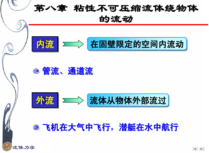
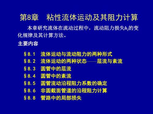
2nd – Year Fluid Mechanics, Faculty of Engineering and Computing, Curtin University FLUID MECHANICS 230For Second-Year Chemical, Civil and Mechanical EngineeringFLUID MECHANICS LECTURE NOTESCHAPTER 8 FLOW OVER IMMERSED BODY8.1 IntroductionWe have discussed pipe flow in Chapter 6, which is internal flow because the fluid is confined within well-defined boundaries. This chapter deals with external flows, i.e. flows over bodies immersed in the fluid. Typical examples of external flows include the flow of water over a submarine (Figure 8-1a) or a fish (Figure 8-1b), the flow of air over an aircraft (Figure 8-1c).(a)(b) (c)Figure 8-1 Examples; a) submarine; b) fish; c) aircraft;The fluid forces (drag and lift) on the immersed bodies are of important considerations in practice. In this chapter, we will learn the fundamentals of drag and lift, as well as the methods for determining and optimising these forces in engineering applications.8.2 Drag and liftAs shown in Figure 8-2, the forces exerted on the surface of an aerofoil by the fluid include the pressure force (Figure 8-2a) and the viscous force (Figure 8-2b). The results of these forces are the net drag force F D and lift force F L (Figure 8-2c). Taking a small element dA on the aerofoil surface in Figure 8-2c, we can decompose the pressure force (PdA ) and viscous force (dA w τ) into x-direction force dF x and y-direction force dF y , as shown in Figure 8-2d,θτθsin )(cos )(dA PdA dF w x += θτθcos )(sin )(dA PdA dF w y +−=.Integrating dF x and dF y along the surface, we can calculate the drag and lift forces as, dA dA P dF F w x D ∫∫∫+==θτθsin cos (E8-1) ∫∫∫+−==dA dA P dF F w y L θτθcos sin . (E8-2)Equations E8-1 and E8-2 reveals that 1) both shear stress and pressure contribute to the drag and lift. In the case of drag, the former is called friction drag ; the later is called pressure drag ;2) to calculate drag and lift, sufficient knowledge are required on three aspects: the body shape as it determines the distribution of θ; the distribution of pressure P and the distribution of shear stress w τ along the surface.Practically, it is very difficult to obtain the distribution of pressure and shear stress. Therefore, E8-1 and E8-2 are generally not very useful. To make it easy for engineers, dimensionless coefficients are often used instead. These dimensionless numbers are called drag coefficient C D and lift coefficient C L , defined as A V F C D D 22ρ= (E8-3) A V F C L L 22ρ= (E8-4) where A is projected (or frontal) area, i.e. the project area of the body in the flow direction.Figure 8-2 Forces on an aerofoil [1]: a) pressure force; b) viscous force; c). resultant drag andlift; d) pressure and viscous forces on a small surface area dA in (c), plotted in an x-y coordination system.8.3 The boundary layer8.3.1 Hydraulician and hydrodynamicistFor a fundamental understanding on the cause of drag and lift, we must have a good understanding on the boundary layer concept. Let’s start with some historical background on two groups of fluid mechanicians who developed two different approaches in dealing with problems of fluid mechanics by late 19th century.One is the group of hydraulicians, focused on experiments and attempted to generalise useful design equations from experimental data. This group developed the filed of experimental hydraulics, delivering empirical solutions with little theoretical content. The other is the group of hydrodynamicists, who focused on differential equations describing flows and tried to apply them to practical problems. In order to solve these differential equations, the fluid was assumed to have zero viscosity and constant density. This group developed the filed of theoretical hydrodynamics, seeking pure theoretical solutions based on ideal-fluid flows.The ideal-fluid solutions of hydrodynamicists agreed well with the observations of flows did not involve solid surface, e.g. tides, however did not agree with observed behaviours in the problems that concerned the hydraulicians, e.g, flow over immersed bodies. The following are two typical examples.(1) Flow over a thin plateFigure 8-3 illustrates the differences between the ideal solutions by the hydrodynamicists and the experimental observations by the hydraulicians for flow over a thin plate. For an ideal-fluid flow (Figure 8-3a), the fluid is inviscid, there is no friction between the fluid and the surface of the thin plate. Therefore, the fluid will maintain its free stream velocity when it flows over the thin plate. However, for a real-fluid flow, the interaction between the viscous fluid with the surface leads to a velocity gradient near the surface of the plate although the fluid far away from the plate still maintains its free stream velocity.(2) Flow over a circular cylinderFigure 8-5 shows the patterns of ideal and real flow over a circular cylinder. In absence of viscous effects, the wall shear stress is zero therefore the streamlines are symmetrical (see Figure 8-6a). The fluid coasts from the front (point A), pasts the top (point C) and then reaches to the rear (point F) of the cylinder.However, the experimental observations by the hydraulicians are very different from the above analysis by the hydrodynamicists, as shown in Figure 8-4b. A real-fluid flow cannot coast along the cylinder surface down to point F. Instead, flow separation occurs from the surface at a point between point C and F, leading to the formation of turbulent wake in the downstream (see Figure 8-4b). The friction between the viscous fluid and the cylinder surface leads to inevitable energy loss so that the flow does not have sufficient kinetic energy to travel along the surface down to the rear of the cylinder.From the above examples, it seems that the hydrodynamicists calculated what can NOT be observed while the hydraulicians observed what can NOT be calculated [2]. By early 20th century, the hydraulicians and hydrodynamicists had completely gone to live in their own worlds. The hydraulicians continued to solve their problems by trial and error based on experiments while the hydrodynamicists kept publishing academic papers based on mathematics with little bearing on engineering problems.(a) Ideal flow over a thin plate(b) Real flow over a thin plateFigure 8-3 Ideal (a) and real (b) flow over a thin plate(a) Ideal flow a cylinder (b) Real turbulent flow over a cylinderFigure 8-4 Ideal (a) and real (b) flow over a cylinder8.3.2 The boundary layer conceptThe revolutionary thinking was finally due in 1904. The two fields of theoretical hydrodynamics and experimental hydraulics were united by a German professor, Ludwig Prandtl (1857-1953). Prandtl proposed the concept of the boundary layer , which has brought the hydrodynamics and hydraulics together and laid the foundation of modern fluid mechanics.F A CTurbulentwakeThe key concept of the boundary layer is to conceptually divide the flow into two regions: •The boundary layer, the region close to solid surfaces, the effects of viscosity are too large to be ignored. Within the boundary layer, ideal-fluid flow is unsatisfactory and a set of boundary layer equations should be used.•Free stream region, the region outside the boundary layer, the effects of viscosity is small and can be neglected. In this region, Ideal-fluid flow is satisfactory.At the edge of boundary layer, the pressures and velocities of the two regions should be matched. Prandtl arbitrarily suggested the boundary layer be considered that region in which the x component of the velocity, v, is less than 0.99 times of the free-stream velocity, V, as shown in Figure 8-5.Figure 8-5 Thickness of the boundary layerThe introduction of the boundary layer concept is revolutionary in seamlessly uniting the fields of theoretical hydrodynamics and experimental hydraulics. The boundary layer concept is commonly accepted as the foundation of modern fluid mechanics, because it has •clarified numerous unexplained phenomena;•provided a much better intellectual basis for discussing complicated flows;•become a standard idea in minds of fluid mechanicians;•brought analogous ideas in heat and mass transfer, generally with useful results. However, it should be noted that•the division of the flow filed by the boundary layer concept does NOT correspond any physically obvious boundary;•the edge of boundary layer does NOT correspond to any sudden change in the flow but rather corresponds to an arbitrary definition;•even with this simplification the calculation is still difficult, and in general only approximate mathematical solutions are possible.Let’s use the boundary layer concept to explain the patterns of flow over a thin plate and flow over a circular cylinder at various Reynolds’ numbers.(1). Flow over a thin plate (Figure 8-6) [1]At a very low Reynolds number, e.g. Re = 0.1 (Figure 8-6a), the viscous force is more important than the inertial force. The viscous effects are therefore strong and the plate affects the flow considerably in a wide range (see the grey area) in all directions. Consequently, there is an extensively wide range around the plate in which the streamlines deflected considerably. The boundary layer is very thick. Outside the boundary layer is the free stream region where viscous effects are no long important so that the ideal-flow solutions is applicable.At a moderate Reynolds number, e.g. Re = 10 (Figure 8-6b), the region in which the viscous effects are important becomes much smaller. The boundary layer is much thinner. The streamlines over the plate only deflected somewhat.At a large Reynolds number, e.g. Re = 107 (Figure 8-6c), the flow is dominated by inertial force. The viscous effects are negligible anywhere except in a thin boundary layer close to the surface of the plate and the wake region. As the boundary layer is very thin, the flow streamlines are largely unaffected except slightly deflected near and within the boundary layer.Figure 8-6 Patterns of flow over a thin plate [1] at (a) a low Reynolds number; (b) a moderate Reynolds number and (c) a large Reynolds numberFigure 8-7 Patterns of flows over a circular cylinder [1] at (a) a low Reynolds number; (b) a moderate Reynolds number and (c) a large Reynolds number2). Flow over a circular cylinder (Figure 8-7) [1]At a low Reynolds number, e.g. Re = 0.1 (Figure 8-7a), flow past a cylinder is dominated by the viscous force. The viscous effects influence a large portion of the flow field, stretching to several diameters in any direction of the cylinder. However, the flow can still coast along the surface of the cylinder slowly. Such flow is sometime called creeping flow, which has streamlines essentially symmetric about the centre of the cylinder.At a moderate Reynolds number, e.g. Re = 50 (Figure 8-7b), the inertial force becomes more important. The region ahead of the cylinder in which the viscous effects are important becomes much smaller. The viscous effects are convected downstream and the flow loses its symmetry. The flow inertia dominates so that it does not coast along the surface down to the rear of the body, resulting in the formation of flow separation bubbles behind the cylinder.At a large Reynolds number, e.g. Re = 105 (Figure 8-6c), the flow is dominated by the inertialforce. The region affected by the viscous forces is forced further downstream, leading to theformation of a very thin boundary layer on the front portion of the cylinder. The boundary lay can be laminar or turbulent, depending on Reynolds number. Due to the strong inertia force, the boundary layer separation occurs from the cylinder, leading to the formation of a turbulent wake region extending far downstream. In the free stream region outside the boundary layer and the wake region, the velocity gradient is zero and the fluid flows as if it were inviscid.8.4 Drag force and streamlined bodies8.4.1 Drag forceIn 1710, Isaac Newton (cited in [2]) dropped hollow spheres from the inside of the dome of St Paul’s Cathedral in London and measured their rate of fall. He calculated that the drag force F D on a sphere and concluded that the following equation holds 242222V D V A F D ρπρ== where A is called projected (or frontal) area – the projected area seen by a person lookingtoward the object from a direction parallel to the upstream (see Figure 8-8).Figure 8-8 Drag force on a free-fall sphereIn other words, Isaac Newton thought that 122=V A F D ρ. However, subsequent experimental investigations by many other researchers found that the above formula must be modified by a coefficient C D in the right-hand side, i.e. D D C V A F =22ρ This is essentially same as the definition of drag coefficient C D in E8-3. Normally, drag coefficient C D is not 1. We can calculate the drag force of the flow on an immersed body as (E8-5)Therefore, when calculate drag force using E8-5, we have accumulated the effects of all rest factors into a single coefficient, C D , i.e. drag coefficient. One can see that the drag coefficient C D in E8-5 plays a similar role of the friction factor f in E6-22. The key difference between E8-5 and E6-22 is that in the case of pipe flow, the geometry of pipes (with different length and diameter) varies while all spheres have the same shape.8.4.2 Drag coefficient chartAccording to E8-1 and the discussion in Section 8-2, the drag coefficient of an object will be a function of Reynolds number, the shape and the surface properties of the object. We haverties)face_prope ,shape,sur Φ(C D Re = (E8-6)Practically, finding the exact function of E8-6 is extremely difficult, if not impossible. Therefore, for engineering applications, what we need is a drag coefficient chart, similar to Moody chart used for determining friction factor in pipe flows. Figure 8-9 shows the dragcoefficient as a function of Reynolds number for a smooth sphere and a smooth cylinder.Figure 8-9 Drag coefficient of a smooth sphere and a smooth circular cylinder [1].EX8-1: An exampleWe caught two breams in two consecutive casts. If we pulled the strings at the same speed, explain why we felt it was much harder to pull the big bream?Solutions:Figure 8-10The projected area of the big bream, A bf , is a much bigger than that of the small bream A sf . As both fishes are bream, we can reasonable assume that the two fishes have similar shape and surface characteristics. As both fishes were caught in consecutive casts in the same water area and we pulled the string at the same speed V , the water flows over the two fishes have same Reynolds numbers. Therefore, the drag coefficients can be taken as same. According to E8-5, the water would have induced much higher drag force on the big bream when we pulled the string.8.4.3 Pressure dragEquation E8-1 in Section 8.2 clearly shows that the drag consists of two components, friction drag and pressure drag. For flow over an immersed circular cylinder, as shown in Figure 8-7c, the fluid friction within the boundary layer certainly leads to the friction drag. In this section, let’s have a detailed analysis on the cause of pressure drag.Let’s start with inviscid flows, as shown in Figure 8-11. In absence of viscosity, the flow will coast along the cylinder surface and the streamlines are symmetrical. Based on theoretical hydrodynamics (further details can be found in Chapter 6 of Reference [1]), the distribution of pressure and velocity along the surface of the cylinder are )sin 41(21220θρ−+=V P P (E8-7) θsin 2V V fs = (E8-8) which are plotted in Figures 8-11b and 8-11c.Figure 8-11c indicates that for an ideal fluid (0=μ and ρ is constant), the fluid velocity along the surface varies from 0=fs V at the very front and rear (stagnation point A and F) of the cylinder to the maximum of V V fs 2= at the bop (point C) and bottom of the cylinder.Figure 8-11 Ideal flow over a circular cylinder [1] (a) streamlines for the ideal flow; (b) pressure distribution of the ideal flow; (c) fluid velocity distribution on the cylinder surfaceFigure 8-12 Real flow over a circular cylinder [1] (a) boundary layer separation; (b)distribution of pressure coefficient.Similarly, as shown in Figure 8-11b, the pressure distribution is also symmetrical about thevertical midplane of the cylinder, varying from a minimum of 2023V P ρ−at the top orbottom of the cylinder to a maximum of 2021V P ρ+. The decrease in pressure in thedirection of flow along the front half of the cylinder is termed as favourable pressure gradientwhile the increase in pressure in the direction of flow along the rear half of the cylinder istermed adverse pressure gradient . In absence of viscous effects, the fluid travelling from thefront to the back of the cylinder coasts down the “pressure hill” (see Figure 8-5b) from°=0θat point A to °=90θat point C and then back up to the hill to °=180θ(from point C topoint F ). Therefore, there is only energy exchange between kinetic energy and pressureenergy without any energy loss.However, the experimental observations are very different from the above theoreticalanalysis, as shown in Figure 8-12. At a large Reynolds number, the flow forms the boundarylayer on the surface of the cylinder and cannot coast along the cylinder surface down to therear stagnation point F. The boundary layer separation occurs at point D on the rear surface, (a)(b)leading to the formation of turbulent wakes in the downstream (see Figure 8-12a). The separation of the boundary layer can be explained by the pressure distribution in Figure 12b. Due to the friction between the viscous fluid and the cylinder surface, energy loss is inevitable so that after pass through point C, the fluid does not have enough kinetic energy to climb the pressure hill up to point F which sits on the top of pressure hill therefore the boundary layer separates at point D in Figure 12a.Figure 8-12b also indicates that the location of separation therefore the width of the turbulent wake and the pressure distribution on the surface depend on the nature of the boundary layer. Compared with a laminar boundary layer, a turbulent boundary layer has more kinetic energy and momentum so that it can flow further around the cylinder, resulting in a narrower wake, less drag, corresponding to a decrease in drag coefficient from point D to E in Figure 8-10. Because of the boundary layer separation, the average pressure on the front half of the cylinder is significantly greater than that on the rear half. This leads to the development of a large pressure drag. Under turbulent conditions, the friction drag is insignificant compared with the pressure drag, as discussed blow.Figure 8-13 Two objects of significant different size that have the same drag force [1]: (a) a circular cylinder - a blunt body, C D = 1.2; (b) a streamlined strut C D = 0.12.Table 8-1 Drag coefficients of various bodies8.4.4 Streamlined bodiesIt is clear now that the drag force developed on an object immersed in turbulent fluid isdominantly pressure drag as a result of boundary layer separation. Therefore, we can optimisethe body shape of the object to minimise the boundary layer separation hence reduce pressuredrag. This requires us to design streamlined bodies .Figure 8-13 shows the significance of body streamlining. The streamlined strut has a sizemuch bigger than the circular cylinder. However, the two bodies have the same drag forces.The boundary layer separation on the streamlined strut has been postponed to the tail of thebody so that pressure drag is minimised compared with that on a circular cylinder, which is ablunt body. It is interesting to revisit the shapes of submarine, fish and aerofoil in Figures 8-1and 8-2, we would appreciate that these bodies are actually all streamlined.8.4.5 Drag coefficient for various objectsThe drag coefficient information for a wide range of objects is available in the literature [1,2].Some of this information is listed in Table 8-1.8.4.6 Drag coefficient at low Reynolds number (Re < 1)At Re < 1, the flow over an immersed body is called creeping flow , dominated by viscouseffects. The drag coefficient gives the 1/Re dependence. Table 8-2 shows the drag coefficientsfor various bodies at Re < 1.Table 8-2 Drag coefficient of various bodies at Re < 1, from Reference [1]8.6 Terminal velocityIf an object in a body of fluid is free to move subject only to gravity, or perhaps centrifugalforces in certain circumstances, then it accelerates to a particular velocity at which the tractiondeveloped and the other forces on the body balance. This velocity is called terminal velocity .Generally, the acceleration is very rapid so that the whole process can be treated as the objecttravelling at the terminal velocity.Figure 8-14a illustrates the concept of terminal velocity of a sphere settling in a fluid. Figure8-14b shows the force analysis of the sphere. When the sphere travels at the terminal velocityV t , the force is balanced. V V V V Re4.20Re6.13Re0.24Re2.22Therefore, as shown in Figure 8-14b, the gravity force F W , drag force F D and buoyancy forceF B are in balance,B D W F F F += (E8-9)We know thatobject object W gV F ρ= (E8-10)object fluid B gV F ρ= (E8-11) projected t fluid D D A V C F 22ρ= (E8-12) where6)2(3433D D V object ππ== (E8-13)42D A projected π=. (E8-14)Assuming Re < 1, for a sphere (see Table 8-2), the drag coefficient is DV C t fluid fluid D ρμ24Re 24==. (E8-15)Substituting E8-15 into E8-12, we have t fluid t fluid t fluid fluid projected t fluid D D DV D V D V A V C F πμπρρμρ342242222===. (E8-16)This is the famous Stock’s law, which is only valid when Re < 1.(a) Concept of terminal velocity (b) Force analysisFigure 8-14 Terminal velocity of a sphereSubstituting E8-11, E8-13 and E8-16 into E8-9, we have fluidfluid object t gD V μρρ18)(2−= (E8-17)Equation E8-17 is not generally given for calculations so that if not available we are requiredto go through the force analysis for its derivation.Once we have calculated the terminal velocity, one final critical step is to double check Re toensure that 0.1Re <=fluid t fluid D V μρ (E8-18)so that our assumption leading to E8-16 is indeed valid.Solutions:We can use a free-body diagram of a mineral particle, as shown in Figure 8-14b. The mineralparticle moves downward with a constant velocity V t (relative to the moving air flow)that isgoverned by a balance between weight of particle, F W , the buoyancy force of the surroundingair, F B , and the drag of air on the particle, F D . Please Note: it is acceptable that thebuoyancy force of the surrounding air, F B , is neglected.(a) We haveB D W F F F += (E8-19)63p p p p W D g gV F πρρ== (E8-20) 63p air p air B D g gV F πρρ== (E8-21)Assuming Re <1, we have the drag coefficient of an mineral particle pt air air D D V C ρμ24Re 24== (E8-22) Therefore the drag force p t air pt air air p t air D p t air D D V D V D V C D V F πμρμπρπρ3244214212222=== (E8-23) Substitute E8-20, E8-21 and E8-23 into E8-19, we have p air p air p p UD D g D g πμπρπρ36633+= Therefore, the terminal velocity of a mineral particle relative to the flowing air is air p air p t gD V μρρ18)(2−= or airp p t gD V μρ182= if buoyancy is neglected,Therefore, we haves m m Ns m s m m kg m kg gD V air p air p t /029.0)/1079.1(18)1020(/8.9)/29.1/2400(18)(25262332=×××××−=−=−−μρρCheck Reynolds number 0.10418.0/1079.11020/029.0/29.1Re 2563<<=××××==−−m Ns m s m m kg D V air p t air μρ Therefore, the assumption to use E8-22 is valid.(b) We can calculate the air travelling velocity in the vertical tube s m m s L m L D Q A Q V tube air /017.0)05.0(14.3)60min 110001min 0.2(44232=××××===π Therefore, the residence time of a mineral particle in the vertical tube is 3.16/)017.0029.0(75.0=+=+=sm m V V L t air t sReferences[1]. Munson BR, Young DF and Okiishi TH, Fundamentals of Fluid Mechanics, 4th Edition,John Wiley & Sons, Brisbane, 2002.[2]. Noel de Nevers, Fluid Mechanics for Chemical Engineers, 3rd Edition, McGraw-Hill’sChemical Engineering Series, Sydney 2005.。
技师培训教材--流体力学(第八章)

v2 代入得: C 1 2 p
或
p v2 C 1 g 2 g
可压缩流体的 伯努利方程
②
p
由于
p 1 p p ① 1 1
RT
③
c
RT
还可得如下不同形式的伯努利方程:
v2 1 p C -----✶) 2 1 p
v2 e C 2 p
-------(✶)
上述一组同等效用,多种形式的伯努利方程的 物理意义:在一元定常等熵气体流动中,沿流束 任意断面上,单位质量气体的机械能和内能之和 保持不变。
二、气体速度与密度的关系
由于 即:
v dv 1
d vdv v 2 dv 2 dv 2 2 Ma c c v v
(3)声速与气体的绝热指数 及气体常数 R 有关。 空气中的声速为:
c 1.4 287T 20.1 T m s
二、马赫数 1、马赫数的定义:气体流动速度 v 与其本身(该 介质中) 的声速 c 之比。 记为:Ma = v / c 马赫数反映了气体的可压缩性程度,是气体 可压缩性效应的一个重要度量。 气体动力学依据马赫数对可压缩气体流动进行分类: Ma 1 即 v c, 为亚声速流动; Ma 1 即 v c, 为(跨)声速流动(兼有亚声速 区和超声速区); Ma >1 即 v > c, 为超声速流动。
气体的全部能量转化为动能,压强为零,速 度达到最大值 vmax,分别称为最大速度状态和最 大速度。
由状态方程可见:因
p
2
RT
T 0 此时 p 0 ,
即 h 0 ,且声速 c 0
2 2 max
流体力学第八章
边界层内
流体力学
v << u
∂u ∂x << ∂u ∂y
普朗特边界层微分方程2
引入无量纲量
t ~1 t′ = l V∞
x x′ = ~ 1 l v ~ δ′ v′ = V∞
δ y y′ = ~ δ ′ = l l
p p′ = ~1 2 ρV∞
u u′ = ~1 V∞
∂u′ ∂v ′ + =0 ∂x ′ ∂y ′
流体力学
顺流平板层流边界层6
1 2 140 μ δ = x+C 2 13 ρV∞
边界条件
x = 0时, δ = 0
μ x δ = 4.641 ρV∞
ρ xV∞ 由 Re x = μ
流体力学
δ = 4.641
x Re x
顺流平板层流边界层7
μ x δ = 4.641 ρV∞ δ = 4.641
x Re x
∗ 0 ∞
U
δ =∫
*
∞ 0
u (1 − )dy U
δ*
μ=0 u=U
边界层内由粘性影响减少的流量=理想流 体流过物面时表面向外移动 δ* 减少的流量
δ =∫
*
δ
0
u (1 − )dy U
流体力学
边界层内的厚度4
动量损失厚度
y dy y
u = u(y)
U
U
θ
μ≠0
μ=0 u=U
边界层内由于粘性的影响,动量流量比 理想流体流经该区域时有所减少
流体力学
8.3 边界层动量积分方程
对控制体的动量方程-近似计算方法
假设 定常不可压 二元边界层 物面曲率很小
B x y U A
8流体力学-第八章 气体一维定常流动

M数很小,说明单位质量气体的动能相对于内能而言很小, 速度的变化不会引起气体温度的显著变化 ,对不可压流体来 说,不仅可以认为密度是常值而且温度T也是常值。
流动参数增加为四个:p、ρ、T、和u,
已经有了三个基本方程,它们是:状态方程、连续方程和理想 流的动量方程(即欧拉方程)。
2021/3/31
19
规
律
26
总结
临界流速达到当地声速cf ,cr kpcr / cr
喷管 dcf>0
Ma<1 dA<0 渐缩
Ma=1 dA=0 临界截面
Ma>1 dA>0 渐扩
Ma<1→Ma>1 dA<0→dA>0 缩放(拉伐尔)
dc f d cf
Ma<1
dc f d cf
dc f d cf
dc f d cf
(c)
在的垂直平面的下游半空间(成为扰动
B
2 3
区)内传播,永远不可能传播到上游半
4
空间(成为寂静区)。
u+c0=2c0 →
3c
2021/3/31
22
2
4
二、亚、超声速流场中小扰动的传播特性
气流A超马声赫锥速流动 Ma>1
vc
vc
由的图扰可动o 见波,不2由 仅c 于 不3c能u>向c0上,游相传对播气,流反传而播被
2)对于气体等可压流,流速的变化取决于截面和密度的综合 变化。超音速时比体积的增加要大于流速的增大,因此,只 有增大通流面积才能保证通过一定不变的质量流量。
一、声速和马赫数
小扰动在弹性介质中的传播速度为声速,气体经历小扰动而压 缩及恢复过程并无能量损耗,作定熵过程处理,对理想气体:
流体力学:第八章 理想不可压缩流体平面流动

因为:ac dy,cb dx,所以
dq udy vdx dy dx d
y x
积分, q
2 d
1
2
1
在论证流函数存在及说明其特性时,仅用了平面 流动的条件,故以上结论对任何平面流动都适用, 不论势流和涡流。
一、无旋流动(有势流动) 旋转角速度为零,通常称为势流。
x
1 ( w 2 y
v ) z
0,
或 w y
v z
y
1 ( u 2 z
w ) 0, x
或 u z
w x
z
1 2
( v x
u ) y
0,
或 v u x y
流体质点本身是否发生旋转,与流体微团 本身运动时的轨迹形状无关。
由数学分析知,上式是使udx vdy wdz为某一函数的
Cylinder with Circulation
引言
平面势流理论在流体力学中占有非常重要的地位 Why? Example
本章将简要地介绍平面势流的基本理论,分析绕流 不同形状的物体势流长的压力分布,以及流体对被绕 流物体的作用力。
§8–1 无旋流动和有旋流动
根据流体微团是否存在旋转,将流动分为两大类型: 无旋流动和有旋流动。 Two examples
涡线
涡线的表达式:
dx dy dz
x y z 通过微元断面的涡线组成涡束,涡束的表面称为涡管。 涡束断面面积和2倍旋转角速度的乘积称为涡通量,以 I表示,则微元涡通量为:
dI 2dA dA
2
速度环量:在流场中取一封闭曲线,流速沿该曲线的
积分称为沿 流线L的速度环量,用 表示:
全微分的必要充分条件。
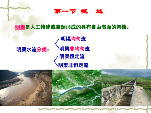
流体力学课件第8章明渠流动
四、水力计算基本问题
主要可归为四大类
1、验算渠道的输水能力。
已知: b, h, m, n, i
以梯形断面 为例分析
求: Q 验算 v 是否
方法: Q Av Ac Ri K i
合乎要求。
2、计算渠道的粗糙系数。
1.天然河道的横断面 呈不规则形状,分主槽和滩地 枯水期:水流过主槽 丰水期:水流过主槽和滩地
主槽
滩地
2、据渠道过流断面的形状、尺寸是否沿程改变:
(1) 棱柱形渠道 A = f (h) ;
A过流断面面积,h水深 (2)非棱柱形渠道 A = f (h,s) s流程
三、明渠的分类
按断面形状、尺寸是否沿程变化分 棱柱体明渠、非棱柱体明渠
2> 设计渠道时,不但应遵从基本公式,还应考虑水 力最优,但由此设计的渠道却不一定是最经济。
断面面积一定时,流量最大为最佳。 流量一定时,断面面积最小为最佳;
(1)最优断面推导——曼宁公式
Q A R1/6 n
Ri 1 A5/3i1/2
n 2/3
思考:相同面积哪种图形周长最小?
当 n、i、A 一定时, 最小,可使 Q 最大,从理论上分
湿周: d 2
水力半径:
R d 1 sin 4
d
h θ
(1) 当а=1 时, 为满管流动;
(2) 当а< 1 时,为不满管流动。在污水管路 设计中,为通风、防暴及适应污水量的变 化,一般均应设计为不满流。
二、水力特征:
Q AC Ri K i
(1) J= Jp= i ;
(2)水力最优发生在满管之前
《流体力学》第八章绕流运动解析

( x, y ) d u dy u y dx C
x
实际上ψ(x,y)表示流场中的流线,C为任 意常数。不同的C,则对应不同的流线。 d dx dy ux , uy x y y x
ux , uy y x
第八章
绕流运动
在自然界和实际工程中,存在着大量的流体 绕流物体的流动问题,即绕流问题。 我们研究时,都是把坐标固结于物体,将物 体看作是静止的,而探讨流体相对于物体的 运动。 在大雷诺数的绕流中,由于流体的惯性力远 大于粘性力,可将流体视为理想流体。 在靠近物体的一薄层内,可以用附面层理论 处理。
d ( x, y, z) ux dx uy dy uz dz
展开势函数的全微分
d dx dy dz x y x
比较上两式的对应系数,得出:
ux uy uz x y z 即速度在三坐标上的投影,等于速度势函 数对于相应坐标的偏导数
工 业 液 槽 边 侧 吸 气
平面无旋运动是旋转角速度为零的平面运 动。在平面运动中,仅只有一个坐标方向 上的旋转角速度分量ωz,当ωz=0时,则 满足: u u
y
x
x
y
这时速度势函数全微分为:
d ux dx u y dy
对应的拉普拉斯方程为: 0 2 2 x y
流函数与势函数间关系为:
ux x y
两者交叉相乘得:
uy y x
0 y y x x
由高等数学得到,上式表明, φ(x,y)=C1和 ψ(x,y)=C2是互为正交的。由此表明:流线与等 势线是相互垂直的。当给出不同的常数C1,C2时, 就可得到一系列等势线和流线,它们间构成相互 正交的流网,应用流网的正交性,借助数值计算 方法和计算机,可以解决复杂的流场问题。
流体力学 第8章
b 2h 1 m
R A
2
(8-5)
水力半径
8.2 明渠均匀流
8.2.3 明渠均匀流的基本公式
均匀流动水头损失计算公式——谢才公式
v C RJ
上式为均匀流的通用公式,既适用于有压管道均匀流, 也适用于明渠均匀流。 对明渠均匀流有 流量
v C Ri
Q Av AC Ri K i
(bhc )3 b 2 hc3 g b
得
hc 3
Q 2
gb
2
3
q 2
g
(8 - 22)
Q 式中,q 称为单宽流量。 b
8.4 明渠流动状态
临界流时的流速是临界流速(vc),由式(8-21)得
Ac vc g Bc
上式与微波速度式相同。
将渠道中的水深 h与临界水深hc相比较,同样可以判 别明渠水流的流动状态,即
8.1 概
述
1 2 i sin l
通常以水平距离lx代替流程长度l,以铅垂断面作为过 流断面,以铅垂深度h作为过流断面的水深,则
1 2 i tan lx
8.1 概
底坡的分类
述
正坡或顺坡:
底线高程沿程降低,i>0
平底坡: 底线高程沿程不变,i=0 反底坡或逆坡:
下游:h → hc < h0,J> i, i-J<0;h→ hc ,Fr
dh 2 →1,1-Fr →0,所以 ds ,水面线与C-C线正交,水
8.6.2 水面曲线分析 实际水深等于正常水深 h=h0时,J=i,分子i-J=0; 实际水深等于临界水深 h=hc时,Fr=1,分母 1-Fr2=0; 分析水面曲线的变化,需 借助h0线(N-N线)和hc线(CC线)将流动空间分区进行。
高等流体力学第八章

指数格式
按上述定义,方程(8.15)变为
J 0 x
(8.18)
对于控制体积内,由上式积分方程可得:
Je J w 0
(8.19)
指数格式
精确解(8.15)可以作为点P与E之间的分布, 其中用 P 和
E 代替 0 和 L
代替L,从而可以给出 J e的表达式:
,并用距离 ( x )e
0 exp( Pe x / L) 1 L 0 exp Pe 1
(8.16)
指数格式
现考虑一个由对流通量密度 u与扩散通量 密度 / x 所组成的总通量密度 J ;
J u x
(8.17)
总通量密度 J 是指单位时间内、单位面积上由扩 散及对流作用而引起的某一物理量的总转移量。
(8.23)
式中,
aP aE aW ( Fe Fw )
(8.24)
Fw exp( Fw / Dw ) aW exp( Fw / Dw ) 1
Fe aE exp( Fe / De ) 1
指数格式
在应用于一维的稳态问题时,指数格式保 证对于任何的Pelclet数以及任意数量的网 格点均可以得到精确解。 缺点: ①指数运算是费时的; ②对于二维或三维的问题,以及源项不为 零的情况,这种方案是不准确的。
控制容积 W w P e E
( δ x )w
( δ x) e
一维问题的典型网格点群
上风方案
上风方案
e P 如果
Fe 0
(8.12a) (8.12b)
e E
如果
Fe 0
上风方案
流体力学 第八章 绕流运动

第八章绕流运动一、应用背景1、问题的广泛存在性:在自然界和工程实际中,存在着大量的流体绕物体的流动问题(绕流问题),如:飞机在空气中的飞行、河水流过桥墩、大型建筑物周围的空气流动、植物护岸(消浪,船行波),粉尘颗粒在空气中的飞扬和沉降,水处理中固体颗粒污染物在水中的运动。
(一种:流体运动;另外一种:物体运动),我们研究,将坐标系固结于物体上,将物体看成静止的,讨论流体相对于物体的运动。
2、问题的复杂性上一章的内容中可以看出,流体力学的问题可以归结为求解在一定边界条件和初始条件下偏微分方程组的求解。
但描述液体运动的方程式非常复杂的:一方面,是方程的非线性性质,造成方程求解的困难;另一方面,复杂的边界条件和初始条件都给求解流体力学造成了很多麻烦。
迄今为止,只有很少数的问题得到了解决。
平面泊萧叶流动,圆管coutte流动等等。
而我们所要解决的绕流问题正是有着非常复杂的边界条件。
3、问题的简化及其合理性流体力学对此的简化则是,简化原方程,建立研究理想液体的势流理论。
实际液体满足势流运动的条件:粘性不占主导地位,或者粘性还没有开始起作用。
正例:远离边界层的流体绕流运动、地下水运动、波浪运动、物体落入静止水体中,水的运动规律研究。
反例:研究阻力规律、能量损失、内能转换等等。
圆柱绕流(经典之一)半无限长平板绕流(经典之二)分成两个区域:一个区域是远离边界的地方,此区域剪切作用不明显,而且流体惯性力的影响远远大于粘性力的影响(理想液体)(引导n-s方程);另一个是靠近边界的地方(附面层,粘性底层),此区域有很强烈的剪切作用,粘性力的影响超强,据现代流体力学的研究表明,此区域是产生湍流的重要区域,有强烈的剪切涡结构,但此区域只有非常薄的厚度。
此区域对绕流物体的阻力、能量耗损、扩散、传热传质都产生重要影响。
4、本章的主要研究内容(1) 外部:理想液体,(简化方法,求解方式)、(2) 内部:附面层理论,(简化方法,求解方式,求解内容,现象描述) (3) 两者的衔接。
第八章不可压缩粘性流体内部流动-流体力学
二、流态与沿程阻力损失的关系
hf的变化规律 hf = kVm
(a)-(b)段,层流,m=1 hf = kV
( d)-(e)段,紊流,m=2 hf = kV2
(b)-(d)段,层流向 紊流过渡
hf = kV1.75~2
三、流态判别标准
雷诺数计算
Re vd vd
上临界Rec′: 与实验条件和初始状态有关。上临界 Rec′可高达13800。(不稳定)
1.紊流结构 层流底层厚度
32.8 d Re
2.混合长度和切应力
(1)粘性切应力
粘性
du dy
普朗特混合长度理论
(2)附加切应力
附加
l 2 ( du )2
dy
紊流切应力
τ= τ粘性+ τ附加 (层流底层τ附加=0)
3.速度分布
层流边层内
du
dy
积分 u 0 y
z2
)
Q(v2
v1 )
g
v2
A2
(v2
v1 )
( z1
p1
)
(
z
2
p2
)
v22 g
v 2 v1 g
代入伯努利方程
hr
v2 2 g
v2v1 g
v12 v2 2 2g
(v1 v2 )2 2g
(包达公式)
hr的另一形式
v1
v2
A2 A1
, 或v2
v1
进一步分析时均流速与脉动速度
《流体力学导论》第八章+对流与扩散-2016.1.7

(1) 如果壁面温度恒定,温度扰动量 如果壁面热流量恒定,温度扰动量 梯度 (2) 固壁上的竖直方向速度扰动量 (3) 扰动量的附加速度边界条件 固壁面(no-slip) : 在 由连续性方程得 自由面(stress-free):在 由连续性方程得 因 有 因 在 在 在
1. 热对流
1.2 Rayleigh-Bé nard 对流
2. 扩散与对流
2.2 描述扩散运动的基本方程
2)分子扩散方程(费克第二定律)
分析分子扩散应满足的控制方程,以一维情况为例,流体静止。 取控制体如图,由质量守恒定律,可得:
(Cx 1) q dt q 1 dt (q x ) 1 dt t x
整理得:
C q 0 t x
或
将费克第一定律代入,可得:
C 2C Dm t x 2
q 2q Dm t x 2
2 2 2 C C C C 2 对三维情况: Dm D C m 2 2 2 t y z x
上述方程称之为分子扩散方程(Diffusion Equations)。
β 流体的浓度扩散系数
2. 扩散与对流
2.3 双扩散对流
基本控制方程
Boussinesq 近似
κT 流体的分子热扩散系数,
κS 流体的分子浓度扩散系数
κT ≠ κS (i)二元组分流体,其中一组分分布受非稳态扰动 (ii)二元组分体流体分别有不同的扩散系数
2. 扩散与对流
2.3 双扩散对流
线性稳定问题 (Linear stability problem): 基本控制方程无量纲化
整理可得:
(Cu1 ) C 2C Dm 2 t x1 x1
流体力学第八章(湍流)

湍流运动极不规则和不稳定,并且每一点的物理量随 时间、空间激烈变化,显然,很难用传统的方法来对湍 流运动加以研究。
但湍流的杂乱无章及随机性可以用概率论及数理统计 的方法加以研究。
也就是说,湍流一方面具有随机性,而另一方面其统 计平均值却符合一定的统计规律。
三、平均值运算法则
①时间平均值:
考虑一维流体运动,对于物理量 A(x, t) ,对于任意空间
点 x ,以某一瞬时 t 为中心,在时间间隔 T 内求平均,
即:
A时
x,
t
1 T
tT
A 2
tT
x, t
dt
2
其中,T 为平均周期,它的选取一般要求大于脉动周期
,而小于流体的特征时间尺度。
②空间平均值:
对于任意时间 t ,以某一空间点 x 为中心,对一定 的空间尺度求平均,即:
A空x, t
Af AdA
而由于物理量量的值通常总是发生一定的有限范围之
内的,故通常采用下式来计算有限范围 A1 ~ A1 内
系统平均值:
A系x, t
A1 Af AdA
A1
以上就是处理湍流运动将经常用到的平均值的定义, 尤其是时间平均用得最多。
定义平均值后,可以将湍流运动表示为: 湍流运动 = 平均运动+脉动运动
为了平均化运算的方便,进行适当变换,可得:
u (uu) (uv) (uw) 1 p 2u u( u v w )
t x y
z
x
x y z
u (uu) (uv) (uw) 1 p 2u
t x y
z
x
将任意物理量表示为: A A A
速度分量为:
u u u;v v v; w w w; p p p
- 1、下载文档前请自行甄别文档内容的完整性,平台不提供额外的编辑、内容补充、找答案等附加服务。
- 2、"仅部分预览"的文档,不可在线预览部分如存在完整性等问题,可反馈申请退款(可完整预览的文档不适用该条件!)。
- 3、如文档侵犯您的权益,请联系客服反馈,我们会尽快为您处理(人工客服工作时间:9:00-18:30)。
MCIS 技术交流
Microsoft
如图,由于气流外折一个角度,流通面积增加,由可压 缩流体连续性方程:
dA dV 2 ( M 1) A V
在超音速气流的情况下,速度增加。 且马赫数增大。
如图,马赫线OL与速度VL夹角就是马赫角θ。取波面控制体 ,联立连续性方程和等熵过程热力学方程,可得:
M 1 dM d 1 M 1 M 2
2 2
凸壁面, dθ>0,dM>0,即马赫数增大,气流加速。 凹壁面,dθ<0,dM<0,即马赫数减小,气流减速。
如果气流连续折过几个微小角 度,则会产生几个马赫波。
如果超音速气流折过一个有限 角△θ,则会产生无数个汇交于 O 点的马赫波,这些发散的马赫波称 为膨胀波。 求得θ与M1、M2的关系式:
c1 RT1
波后的温度从T1增至T1+△T1,波后气体以△V向左运动。 在t=△t~2△t时段,活塞速度增至2△V,产生第二道音波:
c2 R(T1 T1 ) V
MCIS 技术交流
c2>c1,第二道音波很快将赶上第一道音波。
Microsoft
以此类推,第三个微弱扰动波又以比第二个略快一些的声 速向右传播,…。经过一段时间后,后面的微弱扰动波一个一 个追赶上前面的波,波形变得愈来愈陡,最后叠加成一个垂直 于流动方向的具有压强不连续面的压缩波,这就是正激波。
(P P ) ( )
2 2 1 1 2 1
1 ( P2 P )( 2 1 ) 1 Vg VS V2 (1 )VS 2 1 2
如果ρ2→ρ1,P2→P1,激波变成音波 如果P2/P1~∞,则激波的速度也无限大。
例:设在静止大气压强P1=105Pa﹑ρ1=1.28kg/m3,爆炸中心的 P2=5x10⁵Pa,ρ2=3.607kg/m3 则求得的VS=696m/s,Vg=449m/s,V2=247m/s
§ 8.1 膨胀波
当超音速气流中出现微弱压力 扰动时,这个微弱扰动可以传播到 流场的一部分区域,扰动区和未扰 动区的分界面是马赫线(马赫波)。 如果扰动源是一个低压源,则气流受扰动后压强将下降, 速度将增大,这种马赫波称为膨胀波—降压增速波;反之, 如果扰动源是一个高压源,则气流受扰动后压强将增加,速 度将减小,这种马赫波称为压缩波—增压减速波。 由于通过马赫波时气流参数值变化不大,因此气流通过 马赫波的流动仍可作为等熵流动过程。
当出口压强Pb小于入口压强P0时,管内产生流动: 1)设计工况,压强和马赫数沿曲线4变化,出口为超音速; 2)如果气流在喉部到达临界状态后又减速,压强和马赫数沿曲 线3变化,出口为亚音速; 3)Pb的值不是太小时,压强和马赫数沿曲线2变化,整个管内 都是亚声速流动,这时缩放管实际上是文丘里管; 4)非设计工况,如果出口压强大于P4而小于P3,则管内某一截 面产生激波,压强和马赫数沿曲线5变化,气流经过激波后变 成亚音速,在扩张管内进一步减速。
1 arctan M 1 arctan M 1 1 ( M ) ( M )
2 2 2 1
——普朗特-迈耶函数。
§8.2 激波
一.正激波的形成
以气体中的微弱扰动波在直圆管中传播的情况为例来说 明正激波形成的物理过程。 如图所示,在一个充满静止气体的直圆管中,活塞向右 突然加速到某一速度Vg,活塞右侧的静止气体受压后被扰动 形成一个压缩波向右移动,已被扰动的气体的压强从p1升高 到p2。
MCIS 技术交流
Microsoft
设p2- p1是一个有限的压强量。为了分析方便起见,假定把 这个有限的压强增量看作是无数个无限小压强增量dp的总 和。于是,可认为在活塞右侧形成的压缩波是一系列微弱 扰动波连接而成的。每一个微弱扰动波压强增加dp。当活 塞开始运动时,第一个微弱扰动波以声速c1传到未被扰动的 静止气体中去,紧跟着第二个微弱扰动波以声速c2传到已被 第一个微弱扰动波扰动过的气体中去。 在t=0~△t时段,活塞速度增至△V,气体被扰动产生音波 :
激波的性质和原来的各个小压力波有很大的不同。气流通 过激波除压强突跃地升高外,密度和温度也同样突跃地增加, 而速度则下降。激波是以大于其前方气体的声速来传播的。
由于激波是无数道压缩波叠加而成的,使气流的性质发生 质的变化,激波前后参数不再等熵。所以激波与音波有本质的 区别。激波压缩是一个绝热,增熵过程。
§8.3拉瓦尔ห้องสมุดไป่ตู้管
(激波的应用——拉瓦尔管,水垂现象)
拉瓦尔管是瑞典工程师拉瓦尔(de Laval)发明的,用于 产生超音速气流,它由收缩段﹑喉部及扩张段三部分组成,气 流在收缩部分加速,在最小截面(喉部)上达到临界状态,然 后在扩张段继续加速成超音速。整个流动为等熵流动,出口压 强等于背压,不出现激波。
激波的厚度非常小,激波不连续变化是在与气体分子平均 自由行程同一数量级(在空气中约3×10⁻⁴mm左右)内完成的。 例如,在标准大气压、M=2的超音速气流中的激波厚度约为 2.5×10⁻⁵cm。在这个非常小的厚度内,气体的压强﹑密度﹑温 度等发生急剧变化,内部结构很复杂,人们通常忽略其厚度, 认为波面是一个间断面,激波前后的参数发生突跃性的变化。
第八章
膨胀波 激波
膨胀波和激波都是小扰动在超音速气流中传播的物理现 象。所谓小扰动指的是使流动参数发生小变化是个微量,因 而可以略去高阶小量而使得方程线性化。它的特点是扰动以 当地音速传播,扰动波在传播过程中波形不变。
当飞机、炮弹和火箭以超音速飞行时,或者发生强爆炸 、强爆震时,气流受到急剧的压缩,压强和密度发生急剧增 加,这时所产生的压强扰动将以比声速大得多的速度传播, 波阵面所到之处气流的各种参数发生突然的显著变化,产生 突跃,这个强间断面叫做激波阵面。
二.激波的形式
在河道中,当闸门突然打开时,高水位冲向下游,形成 一个水面陡峭水跃区,气体中的激波现象要借助光学等技术 才能观察到。
MCIS 技术交流
Microsoft
三.激波的速度
为了求激波的传播速度Vs,将坐标系x﹑y固定在激波面 上,激波前后的流动参数为:P1﹑T1﹑ρ1和P2﹑T2﹑ρ2 。
连续性方程: V A V A
1 1 2 2
即
1
1VS 2 (Vs Vg )
2 2 2 2 2 1 1
动量方程:( P P ) A V A V A
1 P P2 1V 1 V 2 V 1 1V1 ( 1) 1 2
2
V V
S 1