东南大学-数值分析上机题作业-MATLAB版
数值分析上机作业(MATLAB)

将系数矩阵 A 分解为:A=L+U+D
Ax=b
⇔ (D + L +U)x = b ⇔ Dx = −(L + U )x + b ⇔ x = −D −1(L + U )x + D −1b x(k +1) = −D −1 (L + U ) x(k ) + D −1b
输入 A,b 和初始向量 x
迭代矩阵 BJ , BG
否
ρ(B) < 1?
按雅各比方法进行迭代
否
|| x (k+1) − x(k) ||< ε ?
按高斯-塞德尔法进行迭代
否
|| x(k+1) − x (k ) ||< ε ?
输出迭代结果
图 1 雅各布和高斯-赛德尔算法程序流程图
1.2 问题求解
按图 1 所示的程序流程,用 MATLAB 编写程序代码,具体见附录 1。解上述三个问题 如下
16
-0.72723528355328
0.80813484897616
0.25249261987171
17
-0.72729617968010
0.80805513082418
0.25253982509100
18
-0.72726173942623
0.80809395746552
0.25251408253388
0.80756312717373
8
-0.72715363032573
0.80789064377799
9
-0.72718652854079
数值分析报告上机题课后作业全部-东南大学

实用标准文案文档大全上机作业题报告2015.1.9 USER1.Chapter 11.1题目设S N =∑1j 2−1N j=2,其精确值为)11123(21+--N N 。
(1)编制按从大到小的顺序11131121222-+⋯⋯+-+-=N S N ,计算S N 的通用程序。
(2)编制按从小到大的顺序1211)1(111222-+⋯⋯+--+-=N N S N ,计算S N 的通用程序。
(3)按两种顺序分别计算64210,10,10S S S ,并指出有效位数。
(编制程序时用单精度) (4)通过本次上机题,你明白了什么?1.2程序1.3运行结果1.4结果分析按从大到小的顺序,有效位数分别为:6,4,3。
按从小到大的顺序,有效位数分别为:5,6,6。
可以看出,不同的算法造成的误差限是不同的,好的算法可以让结果更加精确。
当采用从大到小的顺序累加的算法时,误差限随着N 的增大而增大,可见在累加的过程中,误差在放大,造成结果的误差较大。
因此,采取从小到大的顺序累加得到的结果更加精确。
2.Chapter 22.1题目(1)给定初值0x 及容许误差ε,编制牛顿法解方程f(x)=0的通用程序。
(2)给定方程03)(3=-=x xx f ,易知其有三个根3,0,3321=*=*-=*x x x○1由牛顿方法的局部收敛性可知存在,0>δ当),(0δδ+-∈x 时,Newton 迭代序列收敛于根x2*。
试确定尽可能大的δ。
○2试取若干初始值,观察当),1(),1,(),,(),,1(),1,(0+∞+-----∞∈δδδδx 时Newton 序列的收敛性以及收敛于哪一个根。
(3)通过本上机题,你明白了什么?2.2程序2.3运行结果(1)寻找最大的δ值。
算法为:将初值x0在从0开始不断累加搜索精度eps,带入Newton迭代公式,直到求得的根不再收敛于0为止,此时的x0值即为最大的sigma值。
运行Find.m,得到在不同的搜索精度下的最大sigma值。
东南大学数值分析上机题答案
东南⼤学数值分析上机题答案数值分析上机题第⼀章17.(上机题)舍⼊误差与有效数设∑=-=Nj N j S 2211,其精确值为)111-23(21+-N N 。
(1)编制按从⼤到⼩的顺序1-1···1-311-21222N S N +++=,计算N S 的通⽤程序;(2)编制按从⼩到⼤的顺序121···1)1(111222-++--+-=N N S N ,计算NS 的通⽤程序;(3)按两种顺序分别计算210S ,410S ,610S ,并指出有效位数(编制程序时⽤单精度);(4)通过本上机题,你明⽩了什么?解:程序:(1)从⼤到⼩的顺序计算1-1···1-311-21222N S N +++=:function sn1=fromlarge(n) %从⼤到⼩计算sn1format long ; sn1=single(0); for m=2:1:nsn1=sn1+1/(m^2-1); end end(2)从⼩到⼤计算121···1)1(111222-++--+-=N N S N function sn2=fromsmall(n) %从⼩到⼤计算sn2format long ; sn2=single(0); for m=n:-1:2sn2=sn2+1/(m^2-1); end end(3)总的编程程序为: function p203()clear allformat long;n=input('please enter a number as the n:') sn=1/2*(3/2-1/n-1/(n+1));%精确值为sn fprintf('精确值为%f\n',sn);sn1=fromlarge(n);fprintf('从⼤到⼩计算的值为%f\n',sn1);sn2=fromsmall(n);fprintf('从⼩到⼤计算的值为%f\n',sn2);function sn1=fromlarge(n) %从⼤到⼩计算sn1 format long;sn1=single(0);for m=2:1:nsn1=sn1+1/(m^2-1);endendfunction sn2=fromsmall(n) %从⼩到⼤计算sn2 format long;sn2=single(0);for m=n:-1:2sn2=sn2+1/(m^2-1);endendend运⾏结果:从⽽可以得到N值真值顺序值有效位数2 100.740050 从⼤到⼩0.740049 5从⼩到⼤0.740050 64 100.749900 从⼤到⼩0.749852 3从⼩到⼤0.749900 66 100.749999 从⼤到⼩0.749852 3从⼩到⼤0.749999 6(4)感想:通过本上机题,我明⽩了,从⼩到⼤计算数值的精确位数⽐较⾼⽽且与真值较为接近,⽽从⼤到⼩计算数值的精确位数⽐较低。
东南大学Matlab作业3
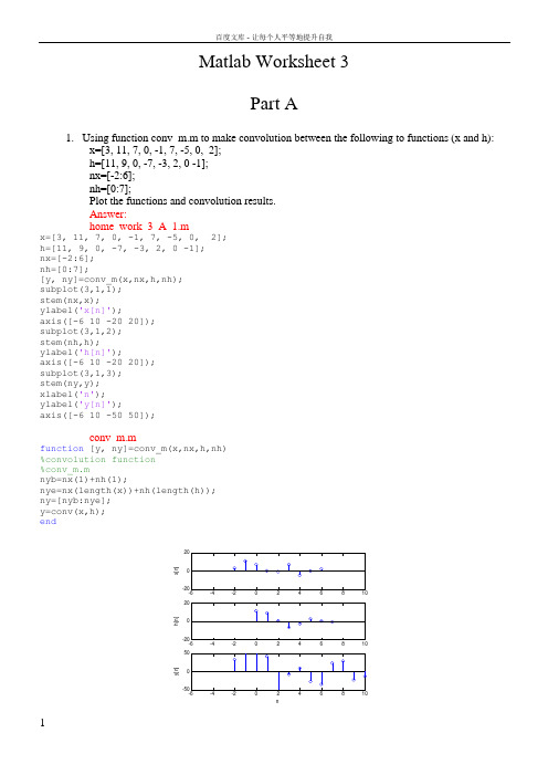
Matlab Worksheet 3Part A1. Using function conv_m.m to make convolution between the following to functions (x and h):x=[3, 11, 7, 0, -1, 7, -5, 0, 2]; h=[11, 9, 0, -7, -3, 2, 0 -1]; nx=[-2:6]; nh=[0:7];Plot the functions and convolution results. Answer:home_work_3_A_1.mx=[3, 11, 7, 0, -1, 7, -5, 0, 2]; h=[11, 9, 0, -7, -3, 2, 0 -1]; nx=[-2:6]; nh=[0:7];[y, ny]=conv_m(x,nx,h,nh); subplot(3,1,1); stem(nx,x); ylabel('x[n]');axis([-6 10 -20 20]);subplot(3,1,2); stem(nh,h); ylabel('h[n]');axis([-6 10 -20 20]); subplot(3,1,3); stem(ny,y); xlabel('n'); ylabel('y[n]');axis([-6 10 -50 50]);conv_m.mfunction [y, ny]=conv_m(x,nx,h,nh) %convolution function %conv_m.mnyb=nx(1)+nh(1);nye=nx(length(x))+nh(length(h)); ny=[nyb:nye]; y=conv(x,h); endx [n ]h [n ]ny [n ]2. Plot the frequency response over π≤Ω≤0for the following transfer function by lettingΩ=j e z , where Ωis the frequency (rad/sample)., with appropriate labels and title.9.06.1)(2++=z z zz H . Answer:home_work_3_A_2.mdelta=0.01;Omega=0:delta:pi; z=exp(j .* Omega);H= z ./ (z.^2+1.6*z+0.9); subplot(2,1,1);plot(Omega, abs(H),'m','LineWidth',2); xlabel('0<\Omega<\pi'); ylabel('|H(\Omega)|');axis([0 pi 0 max(abs(H))]); subplot(2,1,2);plot(Omega,atan2(imag(H),real(H)),'k','LineWidth',2); xlabel('0<\Omega<\pi');ylabel(' -\pi < \Phi_H <\pi') title(' frequency response'); axis([0 pi -pi pi]);0<Ω<π|H (Ω)|0<Ω<π-π < ΦH<π frequency response3. Use fft to analyse following signal by plotting the original signal and its spectrum.⎪⎭⎫ ⎝⎛+⎪⎭⎫ ⎝⎛+⎪⎭⎫ ⎝⎛=10244672sin 10241372sin 1024322sin ][n n n n x πππ.Answer:home_work_3_A_3.m%Examine signal components %sampling rate 1024Hz N=1024; dt=1/N;t=0:dt:1-dt;%****define the signal**x= sin(2*pi*32 .*t) +sin(2*pi*137 .*t )+ sin(2*pi* 467 .*t ) ; %*********************** subplot(2,1,1); plot(t,x);axis([0 1 -1 1]);xlabel('nT (seconds)'); ylabel('x[n]'); X=fft(x); df=1;f=0:df:N-1; subplot(2,1,2); plot(f,abs(X));axis([0 N/2 0 120]); xlabel('k (Hz)'); ylabel('|X[k]|');-1-0.50.5nT (seconds)x [n ]k (Hz)|X [k ]|4. Use the fast Fourier transform function fft to analyse following signal. Plot the original signal, and the magnitude of its spectrum linearly and logarithmically. Apply Hamming window to reduce the leakage.⎪⎭⎫ ⎝⎛+⎪⎭⎫ ⎝⎛+⎪⎭⎫ ⎝⎛=10247.4672sin 10244.1372sin 10245.322sin ][n n n n x πππ.The hamming window can be coded in Matlab asfor n=1:Nhamming(n)=0.54+0.46*cos((2*n-N+1)*pi/N);end;where N is the data length in the FFT.Answer:home_work_3_A_4.m%Windowing for reducing leakage%sampling rate 1024HzN=1024; dt=1/N; t=0:dt:1-dt;%****define the signal**x= sin(2*pi*32.5.*t )+...sin(2*pi*137.4 .*t )+...sin(2*pi*467.7.*t );%***********************% Apply rectangular windowsubplot(3,2,1);plot(t,x);axis([0 1 -5 5]);xlabel('nT (seconds)');ylabel('x[n] rectang win');X=fft(x);df=1;f=0:df:N-1;subplot(3,2,2);plot(f,20*log10(abs(X)));axis([0 N/2 -30 60]);xlabel('k (Hz)');ylabel('|X[k]| (db)');% Apply triangular windowfor n=1:Nw(n)=1-abs(2*n-N+1)/N;end;x1=x .*w;subplot(3,2,3);plot(t,x1);axis([0 1 -5 5]);xlabel('nT (seconds)');ylabel('x[n] triang win');X=fft(x1);df=1;f=0:df:N-1;subplot(3,2,4);plot(f,20*log10(abs(X)));axis([0 N/2 -30 60]);xlabel('k (Hz)');ylabel('|X[k]| (db)');% Apply Hamming windowfor n=1:Nw(n)=0.54+0.46*cos((2*n-N+1)*pi/N); end;x1=x .*w;subplot(3,2,5);plot(t,x1);axis([0 1 -5 5]);xlabel('nT (seconds)');ylabel('x[n] Hamming win');X=fft(x1);df=1;f=0:df:N-1;百度文库 - 让每个人平等地提升自我subplot(3,2,6);plot(f,20*log10(abs(X))); axis([0 N/2 -30 60]); xlabel('k (Hz)');ylabel('|X[k]| (db)');nT (seconds)x [n ] r e c t a n g w i nk (Hz)|X [k ]| (d b)nT (seconds)x [n ] t r i a n g w i nk (Hz)|X[k ]| (d b )nT (seconds)x [n ] H a m m i n g wi nk (Hz)|X [k ]| (d b )Part BSimulation Using SIMULINKINTRODUCTIONThe objective of this laboratory is to learn about various properties of signals and systems by doing simulations in SIMULINK.PART 1. BASICS OF SIMULINK1.1 UNDERSTANDING SIMPLE WAVEFORMS AND INTEGRATIONCreate a pulse of height 2 units from time 0 to 4 seconds by subtracting two unit steps and adding a gain. Connect this pulse to an integrator with a gain of 0.5 and a zero initial condition. Connect oscilloscopes to show the pulse and the output of the integrator. You may wish to name your simulation (block) diagram; to do so use the save as feature under edit. Your block diagram should be similar as below.uBefore simulating you need to pull down the simulation header and double click on parameters. Unless told otherwise always assume that you can use the ode 45 integration algorithm shown in this window and the other default parameters. Typically you will only alter the start and stop times but for this first simulation you can use the default values of 0 and 10 seconds. Double click on the oscilloscopes to get the windows in which the traces will appear, pull down the simulate menu and click on run. Plot below the integrator input and output waveforms.Repeat the experiment but with an initial condition of –2 on the integrator. Again draw the results.1.2 FIRST ORDER SYSTEMA single time constant may be simulated using the transfer function block in which you enter the coefficients of the numerator and denominator polynomials. Set up the configuration in a new SIMULINK window to realise the transfer function 1/(s+2) with the input unit step and an oscilloscope connected to the output of the transfer function block. Plot the block diagram in the space below. Simulate the system for 5 seconds and plot the response.1.3 SECOND ORDER SYSTEMFor the second order all pole transfer function )2/(200220ωωζω++s s you will recall that if a time scale of ω0t is used for plotting the step response, the response shape will only be affected by changes in the damping ratio ζ. This can also be shown if we normalise the transfer function by replacing (s/ω0) by s n togive )12/(12++n ns s ζ. To study the effect of varying ζ on the step response we will therefore use the transfer function 1/(s 2+2ζs+1). Set up the following configuration for a simulation study.i) A unit step input. ii) Connect the unit step to a transfer function of 1/(s 2+2ζs+1) with ζ = 1.0.iii) Take a summing block and connect the input step to a +ve input and the transfer functionoutput to a –ve input. iv) Connect the output of this summer to a square function. This is obtained by using f(u) in thenonlinear blocks. v) Connect the output of this squarer to an integrator. vi) Connect two oscilloscopes to the circuit, one to the transfer function output and the other tothe output of the integrator.vii) Also connect simout blocks to the same signals as the oscilloscopes. Rename the oneconnected to the integrator output simout1.Simulate the system with the values of ζ listed in the table below and fill in the other figures from the simulation results. To get an accurate value at the end of each run you can type simout1 in the MATLAB window. You can also measure the overshoot by making use of the maximum command: simply type max(simout) in the MATLAB window.Table 1 ζ 2.0 1.0 0.9 0.7 0.5 0.3 0.1 0.01 % overshoot 2.1076 1.2500 1.1778 1.0571 1.0000 1.1285 2.1431 3.9651 home_work_3_B_1_3.slxwhen ζ = 1.0:PART 2. SIMULATION OF AIRCRAFT PITCH ANGLE AND ALTITUTE 【pitch :倾斜】The purpose IS to use "SIMULINK" to simulate a (much simplified) model of the longitudinal motion of a fighter aircraft.The "angle of attack", is the angle between the direction a plane is pointing, and the direction in which it actually moves through the air. For a plane flying at approximately constant altitude, this is equivalent to the "pitch angle", φ, as illustrated in Fig.2.1. This angle is important because it produces a lift force perpendicular 【垂直地】 to the axis of the plane, and hence a "normal acceleration", a n , (also shown in the figure).φvNormal Accela nPitch AngleThe pilot wants to be able to control the pitch angle, and does so ultimately by rotating the front fins, and tail elevators of the aircraft, shown in Fig. 2.2. The first task is therefore to model the effect of thesemovements on the "pitch rate" q ( )=φ, and "normal acceleration" a n .Fig. 2.2 Illustration of control surfacesi) Normal Acceleration, a nThe acceleration of the aircraft in a direction perpendicular to its axis, (the "normal accel.", a n ), is determined mainly by the angle θ1 of the tail elevators of the aircraft shown in Fig. 2.2. Indeed aerodynamic modelling shows that this relationship can be described by the differential equation,11116342.364.1982.81.3θθθ++=-+ n n n a a aConvert this relationship into a transfer function form:-ii) Pitch Rate, qThe rate at which the pitch angle changes, (the "pitch rate", q ), is determined mainly by the angle θ2 of the front fins of the aircraft shown in Fig. 2.2. Indeed aerodynamic modelling shows that this relationship can be described by the differential equation,2227.1125.782.81.3θθ++=-+ q q qConvert this relationship into a transfer function form:-iii) Actuator Dynamics + Gears 【齿轮】The tail elevators of the aircraft are driven directly by a hydraulic actuator which has a transfer function,G s s ()()=-+1414/ (3)To a unit step input U(s)=1/s , the response R(s) = G(s)⋅U(s)= 1411)14(14++-=+-s s s s . What form ofstep response r(t) would you expect from this actuator, and what is its time constant?The front fins and the tail elevators are both driven from the actuator by the same drive shaft through a gear box. The same gear on this drive shaft connects to the tail elevator gear wheel, which has 500 teeth, and the front fin gear wheel, which has 100 teeth, the relationship between θ1 and θ2 is52112==t t θθ (4)i) F or the aircraft model you will need from the Continuous or Maths Library:-• a Transfer Fcn block to represent the "tail elevator angle → normal accel" relationship (eqn (1))• a Transfer Fcn block to represent "front fin angle → pitch rate" relationship, (see eqn (2)) • a Transfer Fcn block to represent the hydraulic 【液压的】"actuator dynamics", (see eqn(3))• a Gain block to represent the "gears", (see eqn (4))from the Sources Library:-• a Step Input block to act as a test input - (set Step time = 5sec, and Final value = 0.01 rad) from the Sinks Library:-• a ‘Scope block to monitor the pitch rate output - (set Horizontal Range = 20sec).ii) Now connect the blocks together, using the step input to drive the actuator, and the actuator to drive the tail elevators. The actuator is also used to drive the front fins via the gearbox. The 'Scope should be connected to the output of the "front fin angle → pitch rate" block. Note: you can take a branch from a signal line by dragging with the right mouse button from the point on the line at which you want the branch to start.Plot the block diagram you have created in the box below:-iii) From the pull-down menus of your simulation window, select Simulation/Parameters, in order to define how the simulation is to be performed. Set:Stop Time = 20 sec; Initial Step Size = 0.001; Max Step Size = 0.01;iv) Finally double click on your ‘scope, so that you can watch the progress of the simulation, and then select Simulation/Start from the pull-down menu of your simulation window. You may want to adjust the Vertical Range of your 'Scope, and re-run the simulation to get a good picture. Plot the response of the aircraft pitch rate below, and comment on these results. Note that it can be shown that if a transfer function has a denominator polynomial【分母多项式】 with a zero or negative coefficient then it must have a root with a zero or positive real part.Plot of pitch rate response, to a step change in control input:the tail elevators the front finstest input2.3: SIMULATING THE PITCH RATE CONTROL SYSTEMThe designers are quite glad they simulated the response of the aircraft, before trying it for real. They now decide to improve the response by measuring the output (ie. what is actually happening to the pitch rate), and subtracting this from the input (ie. what they would like to happen), to produce an error signal. The error signal will be amplified, and then used to drive the actuator (see Fig. 2.3). In this way the actuator will automatically act so as to reduce any differences between the input demand, and the output response.Fig. 2.3 Feedbackcontrol of pitchratei) Before yousimulate thecontrol systemdescribed above,you will probably find that you are short of space in your simulation window. Besides it would be nice to package the aircraft + actuator dynamics as a single block, so that they are distinct from anything added later as shown in Fig. 2.3.If you press the left mouse button in an empty space of the window, you get a "rubber band" box which you can drag to surround a group of elements. When you release the button, all elements inside are "selected". Use this technique to select all the aircraft + actuator dynamics, (but leave out the step inputa Subsystem, and yourand ‘scope monitor). From the pull-down menu under Edit select Create ArrayFig. 2.4 New diagramii) Rename the "Subsystem" as "Actuator + Aircraft Dynamics" as shown in Fig. 2.3 by editing the text below the block. You can see what is inside by double clicking on the block itself, - try it! Notice that the input and output connections are labelled "in_1", "out_1" etc. Edit these to give them moremeaningful names.iii) Now construct the planned control system, as illustrated in Fig. 2.3. Notice the pilot is now represented by a Signal Generator (from the Sources library), which should be set to produce a Square Wave, of frequency 0.1 Hz and peak amplitude 0.5.iv) The designers are unsure what value to use for the Gain. Open the Pitch Rate 'Scope, and run the simulation first for the Gain = -0.5 (as shown above), and then for the Gain = -5. Plot the two responses you obtain, and comment on the relative advantages and disadvantages of each:-Plot of pitch rate response, to a square wave in control input:-(a) with Gain = -0.5(b) with Gain = -5Comments on responses (in terms of overshot and response time etc):PART 3: SIMILATION OF NONLINEAR SHIP ROLL DYNAMICSThe rolling motion of ships is of considerable interest to naval architects because even today around 50% of ships lost at sea, sink as a result of a capsize. The aim of this laboratory is to study such behaviour by:-•constructing a nonlinear differential equation model for the system•converting this model into a phase variable block diagram form suitable for simulation•simulating the (nonlinear) response to sinusoidal excitation•calculating the steady state response for a ship whose cargo has shifted dangerously to one sideFig. 3.1 Ship schematic3.1: MODELLING AND SIMULATION OF SHIP DYNAMICSi) Consider the ship sketch shown in Fig. 3.1. Given that:-•The effective inertia 【惯性】of the ship about its roll axis = J (1)• The damping moment 【阻尼力矩】 / torque 【扭矩】 due to friction 【摩擦】between the body of the ship and the water, and due to turbulence 【湍流】 round the "bilge keels" = c c 123 θθ+ (2) • The restoring moment / torque due to the buoyancy 【浮力】 and shape of the ship, as it is pushed to one side = k k k 12335θθθ++ (3) • The input / forcing moment due to the wave forces acting on the ship = u t ()- Using Newton’s second law of motion ∑=Torque Moment J / θ , the nonlinear differential equation which describes the rolling motion of the ship can be written as:-()()53321321)(θθθθθθk k k c c t u J ++-+-= (4)(ii) Re-arrange equation (4) to obtain an expression for the highest derivative of the output signal θ:-()()()53321321)(1θθθθθθk k k c c t u J++-+-= (5)iii) Hence complete the drawing of the SIMULINK block diagram for the ship roll system:-3.2: SIMULATING THE SHIP DYNAMICSi) For the ship model you will need:-from the Continuous and Maths Library:-• a few Integrator blocks - (assume zero initial conditions for now) • a few Gain blocks (not absolutely necessary) from the Nonlinear Library:-• a couple of Fcn blocks to implement the damping and stiffness terms (eqns (2), and (3)) from the Sources Library:-• a Sine Wave block to simulate the sea waves u(t) - (set Ampl = 0.3 , and Freq = 0.6 rad/s) from the Sinks Library:-•a To Workspace block for the output ship roll angle, θ, of the simulation. This stores the results in a MATLAB variable which we can plot later, -(set the Variable name = theta, and the Maximum number of timesteps (ie points stored) = 5000)• an oscilloscope if you wish to see a waveform whilst the simulation is taking placeii) Drag the appropriate blocks over into your simulation window using the mouse, and double click on them to enter the appropriate parameter values. The numerical values for the coefficients of eqn (4) are:-;150;20;8.0;8.0;02.0;132121======k k k c c J (6)Note these values are given in consistent units so that θ is in radians 【弧度】. Finally by clicking on the text under each block, you can also enter a suitable description for each.iii) Now connect the blocks together, according to the phase variable block diagram you have plotted in section A. Note that some blocks will need changing so they "face the other way"; you can do this by selecting the block and "Flipping Horizontally " using the Options pulldown menu. Remember too that you can take a branch from a signal line by dragging with the right mouse button from the point on the line at which you want the branch to start.iv) From the pull-down menus of your simulation window, select Simulation/Parameters , in order to define how the simulation is to be performed. Set:-Stop Time = 10*pi (sec); Initial Step Size = 0.001; Max Step Size = 0.1;v) Now run the simulation by selecting Simulation/Start from the pull-down menu of your simulation window. If you do not use an oscilloscope you probably won't see much happening because the results are being stored in the MATLAB variable called 'theta', instead of being displayed immediately. After a few seconds however, you should hear a slight beep indicating the simulation is complete. Use of an oscilloscope is, however, recommended so that you can see if things ‘look all right’.vi) Now plot your results by typing plot(theta) at the MATLAB prompt in the MATLAB command window. Plot the response below, and comment on how it differs from what you would expect from a linear system if this were also excited with a sine wave input.Display of ship roll response, to a sinusoidal input:-5101520253035-0.4-0.3-0.2-0.100.10.20.3Time (seconds)d a t aTime Series Plot:。
数值分析作业MATLAB
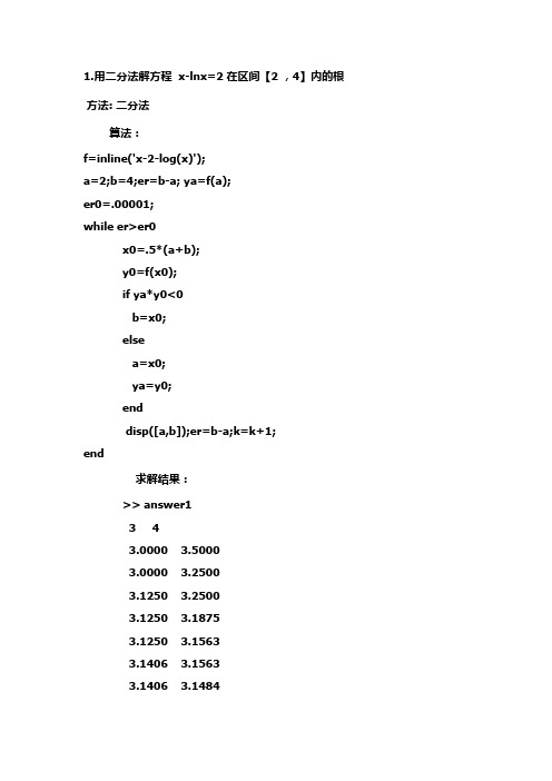
1.用二分法解方程 x-lnx=2 在区间【2 ,4】内的根方法: 二分法算法:f=inline('x-2-log(x)');a=2;b=4;er=b-a; ya=f(a);er0=.00001;while er>er0x0=.5*(a+b);y0=f(x0);if ya*y0<0b=x0;elsea=x0;ya=y0;enddisp([a,b]);er=b-a;k=k+1;end求解结果:>> answer13 43.0000 3.50003.0000 3.25003.1250 3.25003.1250 3.18753.1250 3.15633.1406 3.15633.1406 3.14843.1445 3.1484 3.1445 3.1465 3.1455 3.1465 3.1460 3.1465 3.1460 3.1462 3.1461 3.1462 3.1462 3.14623.1462 3.1462 3.1462 3.1462 3.1462 3.1462 最终结果为: 3.14622.试编写MATLAB 函数实现Newton 插值,要求能输出插值多项式。
对函数141)(2+=x x f 在区间[-5,5]上实现10次多项式插值。
Matlab 程序代码如下:%此函数实现y=1/(1+4*x^2)的n 次Newton 插值,n 由调用函数时指定 %函数输出为插值结果的系数向量(行向量)和插值多项式 算法:function [t y]=func5(n) x0=linspace(-5,5,n+1)'; y0=1./(1.+4.*x0.^2); b=zeros(1,n+1); for i=1:n+1 s=0; for j=1:i t=1; for k=1:iif k~=jt=(x0(j)-x0(k))*t;end;end;s=s+y0(j)/t;end;b(i)=s;end;t=linspace(0,0,n+1);for i=1:ns=linspace(0,0,n+1);s(n+1-i:n+1)=b(i+1).*poly(x0(1:i));t=t+s;end;t(n+1)=t(n+1)+b(1);y=poly2sym(t);10次插值运行结果:[b Y]=func5(10)b =Columns 1 through 4-0.0000 0.0000 0.0027 -0.0000Columns 5 through 8-0.0514 -0.0000 0.3920 -0.0000Columns 9 through 11-1.1433 0.0000 1.0000Y =- (7319042784910035*x^10)/147573952589676412928 + x^9/18446744073709551616 + (256*x^8)/93425 -x^7/1152921504606846976 -(28947735013693*x^6)/562949953421312 -(3*x^5)/72057594037927936 + (36624*x^4)/93425 -(5*x^3)/36028797018963968 -(5148893614132311*x^2)/4503599627370496 +(7*x)/36028797018963968 + 1b为插值多项式系数向量,Y为插值多项式。
数值分析上机题Matlab(东南大学)3
0.22 0.24 0.26 0.28 0.30 0.32 0.34 0.36 0.38 0.40 0.42 0.44 0.46 0.48 0.50 0.52 0.54 0.56 0.58 0.60 0.62 0.64 0.66 0.68 0.70 0.72
152 139 128 119 110 103 96 90 85 80 76 72 68 65 62 59 56 53 51 49 47 45 43 41 39 38
========================================================================================================================
======================================================================================================================================================================== 习题 3_36 ======================================================================================================================================================================== Omega n x1 x2 x3 x4 x5 x6 x7 x8 x9
-0.71279 -0.71280 -0.71280 -0.71280 -0.71280 -0.71280 -0.71280 -0.71280 -0.71280 -0.71280 -0.71280 -0.71281 -0.71281 -0.71281 -0.71281 -0.71281 -0.71281 -0.71281 -0.71281 -0.71281 -0.71281 -0.71281 -0.71281 -0.71281 -0.71281 -0.71281
东南大学Matlab作业1

Matlab Worksheet 1Part A1.Get into Matlab: Use the diary command to record your activity in to a file: diarymydiary01.doc before you start your work. (And diary off to switch off your diary when you finish your work.)At the Command Window assign a v alue x=10, then use the Up Key ↑ to repeat the expression, editing it to show the effect of using a semicolon after the 10, namely x=10;Answers:>> x=10x =10>> x=10;2.Confirm whether the following names of variables are acceptable:a)Velocity Yes Nob)Velocity1 Yes Noc) Velocity.1 Yes Nod)Velocity_1 Yes Noe)Velocity-01 Yes Nof)velocityONE Yes Nog) 1velocity Yes NoAnswers: (1)legal variable names : a) Velocityb) Velocity1d) Velocity_1f) velocityONE(2) illegal variable names: c) Velocity.1e) Velocity-01g) 1velocity3. Assign two scalar variables x and y values x=1.5, y=2.3, then construct Matlab expressions for the following: a) yx y x z +=35 b) ()3/27y x z = c) ()y e x x z 25106/111log -⋅⎥⎦⎤⎢⎣⎡+-= d) )2cos()2sin(x e y x z x ππ+-=Answers:the result of the Command Window is:>> x=1.5;y=2.3 ;z1=5*x^3*y/(x+y)z2=(x^7*y^0.5)^(2/3)z3=(x^(1/6)/(log10(x^5-1))+1)*exp(-2*y)z4=sin(2*pi*x-y)+exp(x).*cos(2*pi*x)z1 =10.2138z2 =8.7566z3 =0.0232z4 =-3.73604. Assign two variables with complex values u=2+3j and v=4+10j and then construct expression for:a) vu b) j uv 2+ c) j u 2 d) u j ve π2- Answers:the result of the Command Window is:>> u=2+3j;v=4+10j;z1=u/vz2=u*v+2jz3=u/2jz4=v*exp(-j*2*pi*u)z1 =0.3276 - 0.0690iz2 =-22.0000 +34.0000iz3 =1.5000 - 1.0000iz4 =6.1421e+08 + 1.5355e+09ie the colon operator : to assign numerical values between 0 and 1 to vector arrayvariable a in steps of 0.1.Answer:the result of the Command Window is:>> V=0:0.1:1V =Columns 1 through 100 0.1000 0.2000 0.3000 0.4000 0.5000 0.6000 0.7000 0.80000.9000Column 111.0000e linspace function to assign 20 values to vector variable y between 20 and 30.Answer:the result of the Command Window is:>> V=linspace(20,30,20)V =Columns 1 through 1020.0000 20.5263 21.0526 21.5789 22.1053 22.6316 23.1579 23.684224.2105 24.7368Columns 11 through 2025.2632 25.7895 26.3158 26.8421 27.3684 27.8947 28.4211 28.947429.4737 30.00007.Assign 20 values to a variable h increasing logarithmically between 10 and 1000.Next, use the colon operator to assign the first 10 elements of h to a variable p.Answers:>> v=logspace(1,3,20)v =1.0e+03 *Columns 1 through 100.0100 0.0127 0.0162 0.0207 0.0264 0.0336 0.0428 0.05460.0695 0.0886Columns 11 through 200.1129 0.1438 0.1833 0.2336 0.2976 0.3793 0.4833 0.61580.7848 1.0000>> p=v(1:10)p =10.0000 12.7427 16.2378 20.6914 26.3665 33.5982 42.8133 54.5559 69.5193 88.58678.Create 6 element row vector z with values 1.0 1.2 1.6 -1.7 1.8 1.9, then constructan expression for the sum of the 2nd 4th and 6th elements of z.Answers:>> z=[1.0 1.2 1.6 -1.7 1.8 1.9]x=z(2)+z(4)+z(6)z =1.0000 1.2000 1.6000 -1.7000 1.8000 1.9000x =1.4000e the colon operator to create a vector array x between 10 and -10in steps of -1,and second, an array vector y between 20 and -20 in steps -2 .a)Add x and y, b) subtract 10x from 5y.Answers:>> x=10:-1:-10y=20:-2:-20x =Columns 1 through 1710 9 8 7 6 5 4 3 2 1 0 -1 -2 -3 -4 -5 -6Columns 18 through 21-7 -8 -9 -10y =Columns 1 through 1720 18 16 14 12 10 8 6 4 2 0 -2 -4 -6 -8 -10 -12 Columns 18 through 21-14 -16 -18 -20>> x+yans =Columns 1 through 1730 27 24 21 18 15 12 9 6 3 0 -3 -6 -9 -12 -15 -18 Columns 18 through 21-21 -24 -27 -30>> 5*y-10*xans =Columns 1 through 170 0 0 0 0 0 0 0 0 0 0 0 0 0 0 0 0Columns 18 through 210 0 0 0e the size,length, who and whos commands to establish the size and length of xand y from Question 9, and use transpose operator ’ to convert vector x fromQuestion 9.Answers:>> size(x)length(x)ans =1 21ans =21>> whoYour variables are:ans x y>> whosName Size Bytes Class Attributesans 1x1 8 doublex 1x21 168 doubley 1x21 168 double>> z=x'z =10987654321-1-2-3-4-5-6-7-8-9-1011.Show that i f w=[ 2i 3i 3+i] the .’ operator creates the transpose. What effect does theoperator ’ applied to w have on its own?Answer:>> w=[ 2i 3i 3+i]w =0 + 2.0000i 0 + 3.0000i 3.0000 + 1.0000i>> x=w'x =0 - 2.0000i0 - 3.0000i3.0000 - 1.0000i>> y=w.'y =0 + 2.0000i0 + 3.0000i3.0000 + 1.0000ie the ones function to create a 4 by 6 array of 1’s. Considering just the shape ofthe resulting array, what do the expression ones(3), ones(5) and ones(7) all have in common?Answer:>> v=ones(4,6)v =1 1 1 1 1 11 1 1 1 1 11 1 1 1 1 11 1 1 1 1 1>> ones(3)ans =1 1 11 1 11 1 1>> ones(5)ans =1 1 1 1 11 1 1 1 11 1 1 1 11 1 1 1 11 1 1 1 1Ones(n)是n阶全为1的方阵13.Create using the rand function a 5 by 4 random matrix and assign it to matrix arrayvariable A and observe carefully what A(:,3) A(1:2) and A(3,[2 4]) mean.Answer:>> A=rand(5,4)A =0.8147 0.0975 0.1576 0.14190.9058 0.2785 0.9706 0.42180.1270 0.5469 0.9572 0.91570.9134 0.9575 0.4854 0.79220.6324 0.9649 0.8003 0.9595>> A(:,3)ans =0.15760.97060.95720.48540.8003>> A(1:2)ans =0.8147 0.9058>> A(3,[2 4])ans =0.5469 0.9157ing array subscripts, create an expression for the sum of the element in the topright-hand-corner of A and the bottom left-hand-corner of A. Also assign the 2nd column of A to a column vector b, and assign the 3rd row of A to a row vector d.Answer:>> A=rand(5,4)A =0.7513 0.9593 0.8407 0.35000.2551 0.5472 0.2543 0.19660.5060 0.1386 0.8143 0.25110.6991 0.1493 0.2435 0.61600.8909 0.2575 0.9293 0.4733>> x=A(1,4)+A(4,1)x =1.0491>> b=A(:,2)b =0.95930.54720.13860.14930.2575>> d=A(3,:)d =0.5060 0.1386 0.8143 0.2511>>diary off to switch off your diary now.15. Using the colon operator, assign a row vector array t, values between 0 and 10 in steps of 0.01. Use the ; operator to prevent displaying the information. Obtain the term-by-term values of functions:a) t e z 05.0-= b) )sin(05.0t e z t π-= c) )2cos()sin(05.0t t e z t ππ-=Answers:(1)home_work_1_A_15.mt=0:0.01:10;z1=exp(-0.05*t)z2=z1.*sin(pi*t)z3=z2.*cos(2*pi*t)(2)result>> home_work_1_A_15z1 =Columns 1 through 101.0000 0.9995 0.9990 0.9985 0.9980 0.9975 0.9970 0.9965 0.9960 0.9955Columns 11 through 200.9950 0.9945 0.9940 0.9935 0.9930 0.9925 0.9920 0.9915 0.9910 0.9905Columns 21 through 300.9900 0.9896 0.9891 0.9886 0.9881 0.9876 0.9871 0.9866 0.9861 0.9856Columns 31 through 400.9851 0.9846 0.9841 0.9836 0.9831 0.9827 0.9822 0.9817 0.9812 0.9807Columns 41 through 500.9802 0.9797 0.9792 0.9787 0.9782 0.9778 0.9773 0.9768 0.9763 0.9758Columns 51 through 600.9753 0.9748 0.9743 0.9738 0.9734 0.9729 0.9724 0.9719 0.9714 0.9709Columns 61 through 700.9704 0.9700 0.9695 0.9690 0.9685 0.9680 0.9675 0.9671 0.9666 0.9661Columns 71 through 800.9656 0.9651 0.9646 0.9642 0.9637 0.9632 0.9627 0.9622 0.9618 0.9613Columns 81 through 900.9608 0.9603 0.9598 0.9593 0.9589 0.9584 0.9579 0.9574 0.9570 0.9565Columns 91 through 1000.9560 0.9555 0.9550 0.9546 0.9541 0.9536 0.9531 0.9527 0.9522 0.9517Columns 101 through 1100.9512 0.9508 0.9503 0.9498 0.9493 0.9489 0.9484 0.9479 0.9474 0.9470Columns 111 through 1200.9465 0.9460 0.9455 0.9451 0.9446 0.9441 0.9436 0.9432 0.9427 0.9422Columns 121 through 1300.9418 0.9413 0.9408 0.9404 0.9399 0.9394 0.9389 0.9385 0.9380 0.9375Columns 131 through 1400.9371 0.9366 0.9361 0.9357 0.9352 0.9347 0.9343 0.9338 0.9333 0.9329Columns 141 through 1500.9324 0.9319 0.9315 0.9310 0.9305 0.9301 0.9296 0.9291 0.9287 0.9282Columns 151 through 1600.9277 0.9273 0.9268 0.9264 0.9259 0.9254 0.9250 0.9245 0.9240 0.9236Columns 161 through 1700.9231 0.9227 0.9222 0.9217 0.9213 0.9208 0.9204 0.9199 0.9194 0.9190Columns 171 through 1800.9185 0.9181 0.9176 0.9171 0.9167 0.9162 0.9158 0.9153 0.9148 0.9144Columns 181 through 1900.9139 0.9135 0.9130 0.9126 0.9121 0.9116 0.9112 0.9107 0.9103 0.9098Columns 191 through 2000.9094 0.9089 0.9085 0.9080 0.9076 0.9071 0.9066 0.9062 0.9057 0.9053Columns 201 through 2100.9048 0.9044 0.9039 0.9035 0.9030 0.9026 0.9021 0.9017 0.9012 0.9008Columns 211 through 2200.9003 0.8999 0.8994 0.8990 0.8985 0.8981 0.8976 0.8972 0.8967 0.8963Columns 221 through 2300.8958 0.8954 0.8949 0.8945 0.8940 0.8936 0.8932 0.8927 0.8923 0.8918Columns 231 through 2400.8914 0.8909 0.8905 0.8900 0.8896 0.8891 0.8887 0.8883 0.8878 0.8874Columns 241 through 2500.8869 0.8865 0.8860 0.8856 0.8851 0.8847 0.8843 0.8838 0.8834 0.8829Columns 251 through 2600.8825 0.8821 0.8816 0.8812 0.8807 0.8803 0.8799 0.8794 0.8790 0.8785Columns 261 through 2700.8781 0.8777 0.8772 0.8768 0.8763 0.8759 0.8755 0.8750 0.8746 0.8742Columns 271 through 2800.8737 0.8733 0.8728 0.8724 0.8720 0.8715 0.8711 0.8707 0.8702 0.8698Columns 281 through 2900.8694 0.8689 0.8685 0.8681 0.8676 0.8672 0.8668 0.8663 0.8659 0.8655Columns 291 through 3000.8650 0.8646 0.8642 0.8637 0.8633 0.8629 0.8624 0.8620 0.8616 0.8611Columns 301 through 3100.8607 0.8603 0.8598 0.8594 0.8590 0.8586 0.8581 0.8577 0.8573 0.8568Columns 311 through 3200.8564 0.8560 0.8556 0.8551 0.8547 0.8543 0.8538 0.8534 0.8530 0.8526Columns 321 through 3300.8521 0.8517 0.8513 0.8509 0.8504 0.8500 0.8496 0.8492 0.8487 0.8483Columns 331 through 3400.8479 0.8475 0.8470 0.8466 0.8462 0.8458 0.8454 0.8449 0.8445 0.8441Columns 341 through 3500.8437 0.8432 0.8428 0.8424 0.8420 0.8416 0.8411 0.8407 0.8403 0.8399Columns 351 through 3600.8395 0.8390 0.8386 0.8382 0.8378 0.8374 0.8369 0.8365 0.8361 0.8357Columns 361 through 3700.8353 0.8349 0.8344 0.8340 0.8336 0.8332 0.8328 0.8324 0.8319 0.8315Columns 371 through 3800.8311 0.8307 0.8303 0.8299 0.8294 0.8290 0.8286 0.8282 0.8278 0.8274Columns 381 through 3900.8270 0.8265 0.8261 0.8257 0.8253 0.8249 0.8245 0.8241 0.8237 0.8232Columns 391 through 4000.8228 0.8224 0.8220 0.8216 0.8212 0.8208 0.8204 0.8200 0.8195 0.8191Columns 401 through 4100.8187 0.8183 0.8179 0.8175 0.8171 0.8167 0.8163 0.8159 0.8155 0.8151Columns 411 through 4200.8146 0.8142 0.8138 0.8134 0.8130 0.8126 0.8122 0.8118 0.8114 0.8110Columns 421 through 4300.8106 0.8102 0.8098 0.8094 0.8090 0.8086 0.8082 0.8078 0.8073 0.8069Columns 431 through 4400.8065 0.8061 0.8057 0.8053 0.8049 0.8045 0.8041 0.8037 0.8033 0.8029Columns 441 through 4500.8025 0.8021 0.8017 0.8013 0.8009 0.8005 0.8001 0.7997 0.7993 0.7989Columns 451 through 4600.7985 0.7981 0.7977 0.7973 0.7969 0.7965 0.7961 0.7957 0.7953 0.7949Columns 461 through 4700.7945 0.7941 0.7937 0.7933 0.7929 0.7925 0.7922 0.7918 0.7914 0.7910Columns 471 through 4800.7906 0.7902 0.7898 0.7894 0.7890 0.7886 0.7882 0.7878 0.7874 0.7870Columns 481 through 4900.7866 0.7862 0.7858 0.7854 0.7851 0.7847 0.7843 0.7839 0.7835 0.7831Columns 491 through 5000.7827 0.7823 0.7819 0.7815 0.7811 0.7808 0.7804 0.7800 0.7796 0.7792Columns 501 through 5100.7788 0.7784 0.7780 0.7776 0.7772 0.7769 0.7765 0.7761 0.7757 0.7753Columns 511 through 5200.7749 0.7745 0.7741 0.7738 0.7734 0.7730 0.7726 0.7722 0.7718 0.7714Columns 521 through 5300.7711 0.7707 0.7703 0.7699 0.7695 0.7691 0.7687 0.7684 0.7680 0.7676Columns 531 through 5400.7672 0.7668 0.7664 0.7661 0.7657 0.7653 0.7649 0.7645 0.7641 0.7638Columns 541 through 5500.7634 0.7630 0.7626 0.7622 0.7619 0.7615 0.7611 0.7607 0.7603 0.7600Columns 551 through 5600.7596 0.7592 0.7588 0.7584 0.7581 0.7577 0.7573 0.7569 0.7565 0.7562Columns 561 through 5700.7558 0.7554 0.7550 0.7547 0.7543 0.7539 0.7535 0.7531 0.7528 0.7524Columns 571 through 5800.7520 0.7516 0.7513 0.7509 0.7505 0.7501 0.7498 0.7494 0.7490 0.7486Columns 581 through 5900.7483 0.7479 0.7475 0.7471 0.7468 0.7464 0.7460 0.7456 0.7453 0.7449Columns 591 through 6000.7445 0.7442 0.7438 0.7434 0.7430 0.7427 0.7423 0.7419 0.7416 0.7412Columns 601 through 6100.7408 0.7404 0.7401 0.7397 0.7393 0.7390 0.7386 0.7382 0.7379 0.7375Columns 611 through 6200.7371 0.7368 0.7364 0.7360 0.7357 0.7353 0.7349 0.7345 0.7342 0.7338Columns 621 through 6300.7334 0.7331 0.7327 0.7323 0.7320 0.7316 0.7312 0.7309 0.7305 0.7302Columns 631 through 6400.7298 0.7294 0.7291 0.7287 0.7283 0.7280 0.7276 0.7272 0.7269 0.7265Columns 641 through 6500.7261 0.7258 0.7254 0.7251 0.7247 0.7243 0.7240 0.7236 0.7233 0.7229Columns 651 through 6600.7225 0.7222 0.7218 0.7214 0.7211 0.7207 0.7204 0.7200 0.7196 0.7193Columns 661 through 6700.7189 0.7186 0.7182 0.7178 0.7175 0.7171 0.7168 0.7164 0.7161 0.7157Columns 671 through 6800.7153 0.7150 0.7146 0.7143 0.7139 0.7136 0.7132 0.7128 0.7125 0.7121Columns 681 through 6900.7118 0.7114 0.7111 0.7107 0.7103 0.7100 0.7096 0.7093 0.7089 0.7086Columns 691 through 7000.7082 0.7079 0.7075 0.7072 0.7068 0.7065 0.7061 0.7057 0.7054 0.7050Columns 701 through 7100.7047 0.7043 0.7040 0.7036 0.7033 0.7029 0.7026 0.7022 0.7019 0.7015Columns 711 through 7200.7012 0.7008 0.7005 0.7001 0.6998 0.6994 0.6991 0.6987 0.6984 0.6980Columns 721 through 7300.6977 0.6973 0.6970 0.6966 0.6963 0.6959 0.6956 0.6952 0.6949 0.6945Columns 731 through 7400.6942 0.6938 0.6935 0.6932 0.6928 0.6925 0.6921 0.6918 0.6914 0.6911Columns 741 through 7500.6907 0.6904 0.6900 0.6897 0.6894 0.6890 0.6887 0.6883 0.6880 0.6876Columns 751 through 7600.6873 0.6869 0.6866 0.6863 0.6859 0.6856 0.6852 0.6849 0.6845 0.6842Columns 761 through 7700.6839 0.6835 0.6832 0.6828 0.6825 0.6822 0.6818 0.6815 0.6811 0.6808Columns 771 through 7800.6805 0.6801 0.6798 0.6794 0.6791 0.6788 0.6784 0.6781 0.6777 0.6774Columns 781 through 7900.6771 0.6767 0.6764 0.6760 0.6757 0.6754 0.6750 0.6747 0.6744 0.6740Columns 791 through 8000.6737 0.6733 0.6730 0.6727 0.6723 0.6720 0.6717 0.6713 0.6710 0.6707Columns 801 through 8100.6703 0.6700 0.6697 0.6693 0.6690 0.6686 0.6683 0.6680 0.6676 0.6673Columns 811 through 8200.6670 0.6666 0.6663 0.6660 0.6656 0.6653 0.6650 0.6646 0.6643 0.6640Columns 821 through 8300.6637 0.6633 0.6630 0.6627 0.6623 0.6620 0.6617 0.6613 0.6610 0.6607Columns 831 through 8400.6603 0.6600 0.6597 0.6594 0.6590 0.6587 0.6584 0.6580 0.6577 0.6574Columns 841 through 8500.6570 0.6567 0.6564 0.6561 0.6557 0.6554 0.6551 0.6548 0.6544 0.6541Columns 851 through 8600.6538 0.6534 0.6531 0.6528 0.6525 0.6521 0.6518 0.6515 0.6512 0.6508Columns 861 through 8700.6505 0.6502 0.6499 0.6495 0.6492 0.6489 0.6486 0.6482 0.6479 0.6476Columns 871 through 8800.6473 0.6469 0.6466 0.6463 0.6460 0.6456 0.6453 0.6450 0.6447 0.6444Columns 881 through 8900.6440 0.6437 0.6434 0.6431 0.6427 0.6424 0.6421 0.6418 0.6415 0.6411Columns 891 through 9000.6408 0.6405 0.6402 0.6399 0.6395 0.6392 0.6389 0.6386 0.6383 0.6379Columns 901 through 9100.6376 0.6373 0.6370 0.6367 0.6364 0.6360 0.6357 0.6354 0.6351 0.6348Columns 911 through 9200.6344 0.6341 0.6338 0.6335 0.6332 0.6329 0.6325 0.6322 0.6319 0.6316Columns 921 through 9300.6313 0.6310 0.6307 0.6303 0.6300 0.6297 0.6294 0.6291 0.6288 0.6284Columns 931 through 9400.6281 0.6278 0.6275 0.6272 0.6269 0.6266 0.6263 0.6259 0.6256 0.6253Columns 941 through 9500.6250 0.6247 0.6244 0.6241 0.6238 0.6234 0.6231 0.6228 0.6225 0.6222Columns 951 through 9600.6219 0.6216 0.6213 0.6210 0.6206 0.6203 0.6200 0.6197 0.6194 0.6191Columns 961 through 9700.6188 0.6185 0.6182 0.6179 0.6175 0.6172 0.6169 0.6166 0.6163 0.6160Columns 971 through 9800.6157 0.6154 0.6151 0.6148 0.6145 0.6142 0.6139 0.6135 0.6132 0.6129Columns 981 through 9900.6126 0.6123 0.6120 0.6117 0.6114 0.6111 0.6108 0.6105 0.6102 0.6099Columns 991 through 10000.6096 0.6093 0.6090 0.6087 0.6084 0.6080 0.6077 0.6074 0.6071 0.6068Column 10010.6065z2 =Columns 1 through 100 0.0314 0.0627 0.0940 0.1251 0.1560 0.1868 0.2174 0.2477 0.2777Columns 11 through 200.3075 0.3369 0.3659 0.3946 0.4228 0.4506 0.4779 0.5047 0.5310 0.5568Columns 21 through 300.5819 0.6065 0.6305 0.6538 0.6764 0.6983 0.7196 0.7401 0.7598 0.7788Columns 31 through 400.7970 0.8144 0.8309 0.8467 0.8615 0.8755 0.8887 0.9009 0.9123 0.9227Columns 41 through 500.9322 0.9408 0.9485 0.9552 0.9609 0.9657 0.9696 0.9724 0.9744 0.9753Columns 51 through 600.9753 0.9743 0.9724 0.9695 0.9657 0.9609 0.9552 0.9485 0.9409 0.9324Columns 61 through 700.9229 0.9126 0.9014 0.8893 0.8763 0.8625 0.8479 0.8324 0.8161 0.7990Columns 71 through 800.7812 0.7626 0.7433 0.7232 0.7025 0.6811 0.6590 0.6363 0.6130 0.5892Columns 81 through 900.5647 0.5398 0.5143 0.4883 0.4619 0.4351 0.4079 0.3802 0.3523 0.3240Columns 91 through 1000.2954 0.2666 0.2375 0.2082 0.1788 0.1492 0.1195 0.0897 0.0598 0.0299Columns 101 through 1100.0000 -0.0299 -0.0597 -0.0894 -0.1190 -0.1484 -0.1777 -0.2068 -0.2356 -0.2642Columns 111 through 120-0.2925 -0.3205 -0.3481 -0.3753 -0.4022 -0.4286 -0.4546 -0.4801 -0.5051 -0.5296Columns 121 through 130-0.5536 -0.5769 -0.5997 -0.6219 -0.6434 -0.6643 -0.6845 -0.7040 -0.7227 -0.7408Columns 131 through 140-0.7581 -0.7746 -0.7904 -0.8054 -0.8195 -0.8328 -0.8453 -0.8570 -0.8678 -0.8777Columns 141 through 150-0.8868 -0.8949 -0.9022 -0.9086 -0.9140 -0.9186 -0.9223 -0.9250 -0.9268 -0.9277Columns 151 through 160-0.9277 -0.9268 -0.9250 -0.9222 -0.9186 -0.9140 -0.9086 -0.9022 -0.8950 -0.8869Columns 161 through 170-0.8779 -0.8681 -0.8574 -0.8459 -0.8336 -0.8204 -0.8065 -0.7918 -0.7763 -0.7601Columns 171 through 180-0.7431 -0.7254 -0.7070 -0.6880 -0.6682 -0.6479 -0.6269 -0.6053 -0.5831 -0.5604Columns 181 through 190-0.5372 -0.5134 -0.4892 -0.4645 -0.4394 -0.4139 -0.3880 -0.3617 -0.3351 -0.3082Columns 191 through 200-0.2810 -0.2536 -0.2259 -0.1981 -0.1701 -0.1419 -0.1136 -0.0853 -0.0569 -0.0284Columns 201 through 210-0.0000 0.0284 0.0568 0.0850 0.1132 0.1412 0.1690 0.1967 0.2241 0.2513Columns 211 through 2200.2782 0.3048 0.3311 0.3570 0.3826 0.4077 0.4324 0.4567 0.4805 0.5038Columns 221 through 2300.5266 0.5488 0.5705 0.5915 0.6120 0.6319 0.6511 0.6696 0.6875 0.7047Columns 231 through 2400.7211 0.7369 0.7519 0.7661 0.7795 0.7922 0.8041 0.8152 0.8255 0.8349Columns 241 through 2500.8435 0.8513 0.8582 0.8643 0.8695 0.8738 0.8773 0.8799 0.8816 0.8825Columns 251 through 2600.8825 0.8816 0.8799 0.8773 0.8738 0.8695 0.8643 0.8582 0.8514 0.8437Columns 261 through 2700.8351 0.8258 0.8156 0.8047 0.7929 0.7804 0.7672 0.7532 0.7384 0.7230Columns 271 through 2800.7069 0.6900 0.6725 0.6544 0.6356 0.6163 0.5963 0.5758 0.5547 0.5331Columns 281 through 2900.5110 0.4884 0.4654 0.4419 0.4180 0.3937 0.3690 0.3441 0.3188 0.2932Columns 291 through 3000.2673 0.2412 0.2149 0.1884 0.1618 0.1350 0.1081 0.0811 0.0541 0.0270Columns 301 through 3100.0000 -0.0270 -0.0540 -0.0809 -0.1077 -0.1343 -0.1608 -0.1871 -0.2132 -0.2391Columns 311 through 320-0.2646 -0.2900 -0.3150 -0.3396 -0.3639 -0.3878 -0.4113 -0.4344 -0.4571 -0.4792Columns 321 through 330-0.5009 -0.5220 -0.5426 -0.5627 -0.5822 -0.6011 -0.6193 -0.6370 -0.6540 -0.6703Columns 331 through 340-0.6860 -0.7009 -0.7152 -0.7287 -0.7415 -0.7536 -0.7649 -0.7754 -0.7852 -0.7942Columns 341 through 350-0.8024 -0.8098 -0.8163 -0.8221 -0.8271 -0.8312 -0.8345 -0.8370 -0.8386 -0.8395Columns 351 through 360-0.8395 -0.8386 -0.8370 -0.8345 -0.8312 -0.8271 -0.8221 -0.8164 -0.8098 -0.8025Columns 361 through 370-0.7944 -0.7855 -0.7758 -0.7654 -0.7543 -0.7424 -0.7298 -0.7164 -0.7024 -0.6877Columns 371 through 380-0.6724 -0.6564 -0.6397 -0.6225 -0.6046 -0.5862 -0.5672 -0.5477 -0.5277 -0.5071Columns 381 through 390-0.4861 -0.4646 -0.4427 -0.4203 -0.3976 -0.3745 -0.3510 -0.3273 -0.3032 -0.2789Columns 391 through 400-0.2543 -0.2294 -0.2044 -0.1792 -0.1539 -0.1284 -0.1028 -0.0772 -0.0515 -0.0257Columns 401 through 410-0.0000 0.0257 0.0514 0.0769 0.1024 0.1278 0.1530 0.1780 0.2028 0.2274Columns 411 through 4200.2517 0.2758 0.2996 0.3231 0.3462 0.3689 0.3913 0.4132 0.4348 0.4558Columns 421 through 4300.4764 0.4966 0.5162 0.5352 0.5538 0.5717 0.5891 0.6059 0.6221 0.6376Columns 431 through 4400.6525 0.6667 0.6803 0.6932 0.7054 0.7168 0.7276 0.7376 0.7469 0.7555Columns 441 through 4500.7632 0.7703 0.7765 0.7820 0.7867 0.7907 0.7938 0.7962 0.7977 0.7985Columns 451 through 4600.7985 0.7977 0.7961 0.7938 0.7906 0.7867 0.7820 0.7766 0.7703 0.7634Columns 461 through 4700.7556 0.7472 0.7380 0.7281 0.7175 0.7062 0.6942 0.6815 0.6682 0.6542Columns 471 through 4800.6396 0.6244 0.6085 0.5921 0.5751 0.5576 0.5396 0.5210 0.5019 0.4824Columns 481 through 4900.4624 0.4419 0.4211 0.3998 0.3782 0.3562 0.3339 0.3113 0.2884 0.2653Columns 491 through 5000.2419 0.2183 0.1945 0.1705 0.1464 0.1221 0.0978 0.0734 0.0490 0.0245Columns 501 through 5100.0000 -0.0245 -0.0489 -0.0732 -0.0974 -0.1215 -0.1455 -0.1693 -0.1929 -0.2163Columns 511 through 520-0.2395 -0.2624 -0.2850 -0.3073 -0.3293 -0.3509 -0.3722 -0.3931 -0.4136 -0.4336Columns 521 through 530-0.4532 -0.4723 -0.4910 -0.5091 -0.5268 -0.5439 -0.5604 -0.5764 -0.5917 -0.6065Columns 531 through 540-0.6207 -0.6342 -0.6471 -0.6594 -0.6710 -0.6819 -0.6921 -0.7016 -0.7105 -0.7186Columns 541 through 550-0.7260 -0.7327 -0.7387 -0.7439 -0.7484 -0.7521 -0.7551 -0.7573 -0.7588 -0.7596Columns 551 through 560-0.7596 -0.7588 -0.7573 -0.7551 -0.7521 -0.7483 -0.7439 -0.7387 -0.7328 -0.7261Columns 561 through 570-0.7188 -0.7107 -0.7020 -0.6926 -0.6825 -0.6717 -0.6603 -0.6483 -0.6356 -0.6223Columns 571 through 580-0.6084 -0.5939 -0.5789 -0.5632 -0.5471 -0.5304 -0.5132 -0.4956 -0.4774 -0.4588Columns 581 through 590-0.4398 -0.4204 -0.4005 -0.3803 -0.3598 -0.3389 -0.3176 -0.2961 -0.2744 -0.2523Columns 591 through 600-0.2301 -0.2076 -0.1850 -0.1622 -0.1392 -0.1162 -0.0930 -0.0698 -0.0466 -0.0233Columns 601 through 610-0.0000 0.0233 0.0465 0.0696 0.0927 0.1156 0.1384 0.1610 0.1835 0.2058Columns 611 through 6200.2278 0.2496 0.2711 0.2923 0.3132 0.3338 0.3540 0.3739 0.3934 0.4125Columns 621 through 6300.4311 0.4493 0.4670 0.4843 0.5011 0.5173 0.5331 0.5482 0.5629 0.5769Columns 631 through 6400.5904 0.6033 0.6156 0.6272 0.6382 0.6486 0.6584 0.6674 0.6758 0.6836Columns 641 through 6500.6906 0.6970 0.7026 0.7076 0.7119 0.7154 0.7183 0.7204 0.7218 0.7225Columns 651 through 6600.7225 0.7218 0.7204 0.7182 0.7154 0.7118 0.7076 0.7027 0.6970 0.6907Columns 661 through 6700.6837 0.6761 0.6678 0.6588 0.6492 0.6390 0.6281 0.6166 0.6046 0.5919Columns 671 through 6800.5787 0.5649 0.5506 0.5358 0.5204 0.5046 0.4882 0.4714 0.4542 0.4365Columns 681 through 6900.4184 0.3999 0.3810 0.3618 0.3422 0.3223 0.3021 0.2817 0.2610 0.2400Columns 691 through 7000.2189 0.1975 0.1760 0.1543 0.1324 0.1105 0.0885 0.0664 0.0443 0.0221Columns 701 through 7100.0000 -0.0221 -0.0442 -0.0662 -0.0881 -0.1100 -0.1316 -0.1532 -0.1745 -0.1957Columns 711 through 720-0.2167 -0.2374 -0.2579 -0.2781 -0.2979 -0.3175 -0.3368 -0.3557 -0.3742 -0.3923Columns 721 through 730-0.4101 -0.4274 -0.4443 -0.4607 -0.4766 -0.4921 -0.5071 -0.5215 -0.5354 -0.5488Columns 731 through 740-0.5616 -0.5739 -0.5855 -0.5966 -0.6071 -0.6170 -0.6262 -0.6349 -0.6429 -0.6502Columns 741 through 750-0.6569 -0.6630 -0.6684 -0.6731 -0.6771 -0.6805 -0.6832 -0.6853 -0.6866 -0.6873Columns 751 through 760-0.6873 -0.6866 -0.6852 -0.6832 -0.6805 -0.6771 -0.6731 -0.6684 -0.6630 -0.6570Columns 761 through 770-0.6504 -0.6431 -0.6352 -0.6267 -0.6175 -0.6078 -0.5975 -0.5866 -0.5751 -0.5631Columns 771 through 780-0.5505 -0.5374 -0.5238 -0.5096 -0.4950 -0.4799 -0.4644 -0.4484 -0.4320 -0.4152Columns 781 through 790-0.3980 -0.3804 -0.3624 -0.3441 -0.3255 -0.3066 -0.2874 -0.2680 -0.2482 -0.2283Columns 791 through 800-0.2082 -0.1879 -0.1674 -0.1467 -0.1260 -0.1051 -0.0842 -0.0632 -0.0421 -0.0211Columns 801 through 810-0.0000 0.0210 0.0420 0.0630 0.0838 0.1046 0.1252 0.1457 0.1660 0.1862Columns 811 through 8200.2061 0.2258 0.2453 0.2645 0.2834 0.3020 0.3204 0.3383 0.3560 0.3732Columns 821 through 8300.3901 0.4066 0.4226 0.4382 0.4534 0.4681 0.4823 0.4961 0.5093 0.5220Columns 831 through 8400.5342 0.5459 0.5570 0.5675 0.5775 0.5869 0.5957 0.6039 0.6115 0.6185Columns 841 through 8500.6249 0.6306 0.6358 0.6403 0.6441 0.6473 0.6499 0.6518 0.6531 0.6538Columns 851 through 8600.6538 0.6531 0.6518 0.6499 0.6473 0.6441 0.6403 0.6358 0.6307 0.6250Columns 861 through 8700.6187 0.6117 0.6042 0.5961 0.5874 0.5782 0.5683 0.5580 0.5471 0.5356Columns 871 through 8800.5236 0.5112 0.4982 0.4848 0.4709 0.4565 0.4418 0.4265 0.4109 0.3949Columns 881 through 8900.3786 0.3618 0.3447 0.3273 0.3096 0.2917 0.2734 0.2549 0.2361 0.2172Columns 891 through 9000.1980 0.1787 0.1592 0.1396 0.1198 0.1000 0.0801 0.0601 0.0401 0.0200Columns 901 through 9100.0000 -0.0200 -0.0400 -0.0599 -0.0798 -0.0995 -0.1191 -0.1386 -0.1579 -0.1771Columns 911 through 920-0.1961 -0.2148 -0.2333 -0.2516 -0.2696 -0.2873 -0.3047 -0.3218 -0.3386 -0.3550Columns 921 through 930-0.3711 -0.3867 -0.4020 -0.4168 -0.4313 -0.4453 -0.4588 -0.4719 -0.4845 -0.4966Columns 931 through 940-0.5082 -0.5193 -0.5298 -0.5399 -0.5493 -0.5583 -0.5667 -0.5745 -0.5817 -0.5883Columns 941 through 950-0.5944 -0.5999 -0.6048 -0.6090 -0.6127 -0.6158 -0.6182 -0.6201 -0.6213 -0.6219Columns 951 through 960-0.6219 -0.6213 -0.6200 -0.6182 -0.6157 -0.6127 -0.6090 -0.6048 -0.5999 -0.5945Columns 961 through 970-0.5885 -0.5819 -0.5748 -0.5670 -0.5588 -0.5500 -0.5406 -0.5308 -0.5204 -0.5095Columns 971 through 980-0.4981 -0.4863 -0.4739 -0.4611 -0.4479 -0.4343 -0.4202 -0.4057 -0.3909 -0.3757Columns 981 through 990-0.3601 -0.3442 -0.3279 -0.3114 -0.2945 -0.2774 -0.2601 -0.2425 -0.2246 -0.2066Columns 991 through 1000-0.1884 -0.1700 -0.1514 -0.1328 -0.1140 -0.0951 -0.0762 -0.0572 -0.0381 -0.0191Column 1001-0.0000z3 =Columns 1 through 100 0.0313 0.0622 0.0923 0.1212 0.1484 0.1737 0.1967 0.2171 0.2345Columns 11 through 200.2488 0.2596 0.2667 0.2701 0.2695 0.2649 0.2561 0.2432 0.2261 0.2050Columns 21 through 300.1798 0.1508 0.1181 0.0819 0.0425 0.0000 -0.0452 -0.0928 -0.1424 -0.1937Columns 31 through 40-0.2463 -0.2998 -0.3538 -0.4079 -0.4616 -0.5146 -0.5665 -0.6167 -0.6650 -0.7110Columns 41 through 50-0.7542 -0.7944 -0.8311 -0.8643 -0.8934 -0.9184 -0.9391 -0.9552 -0.9667 -0.9734Columns 51 through 60-0.9753 -0.9724 -0.9647 -0.9524 -0.9353 -0.9139 -0.8881 -0.8582 -0.8245 -0.7872Columns 61 through 70。
数值计算上机实习题目(matlab编程)
数值计算上机实习题目(matlab编程)非线性方程求根一、实验目的本次实验通过上机实习,了解迭代法求解非线性方程数值解的过程和步骤。
二、实验要求1、用迭代法求方程230x x e -=的根。
要求:确定迭代函数?(x),使得x=?(x),并求一根。
提示:构造迭代函数2ln(3)x ?=。
2、对上面的方程用牛顿迭代计算。
3、用割线法求方程3()310f x x x =--=在02x =附近的根。
误差限为410-,取012, 1.9x x ==。
三、实验内容1、(1)首先编写迭代函数,记为iterate.mfunction y=iterate(x)x1=g(x); % x 为初始值。
n=1;while(abs(x1-x)>=1.0e-6)&(n<=1000) % 迭代终止的原则。
x=x1;x1=g(x);n=n+1;endx1 %近似根n %迭代步数(2)后编制函数文件?(x),记为g.mfunction y=g(x)y=log(3*x.^2);(3)设初始值为0、3、-3、1000,观察初始值对求解的影响。
将结果记录在文档中。
>>iterate(0)>>iterate(3) 等等2、(1)首先编制牛顿迭代函数如下,记为newton.mfunction y=newton(x0)x1=x0-fc(x0)/df(x0); % 牛顿迭代格式n=1;while(abs(x1-x0)>=1.0e-6)&(n<=1000000) % 迭代终止的原则。
x0=x1;x1=x0-fc(x0)/df(x0);n=n+1;endx1 %近似根n %迭代步数(2)对题目中的方程编制函数文件,记为fc.mfunction y=fc(x)y=3*x.^2-exp(x)编制函数的导数文件,记为df.mfunction y=df(x)y=6*x-exp(x)(3)在MATLAB 命令窗计算,当设初始值为0时,newton(0);给定不同的初始值,观察用牛顿法求解时所需要的迭代步数,并与上面第一题的迭代步数比较。
东南大学数值分析--精选上机作业汇总--精选.doc

在x0∈(-1,
)区间,取以下初值,分别调用
newton.m函数文件,得到
结果如下:
X0
X1
迭代次数
-0.95
1.732051
9
-0.85
1.732051
6
-0.80
1.732051
10
-0.78
1.732051
0.0000005
由newton1.m的运行过程表明,在整个区间上均收敛于0,即根x*2。
在x0∈(,1)区间,取以下初值,分别调用newton.m函数文件,得到结果如下:
X0
X1
迭代次数
0.80
-1.732051
10
0.90
-1.732051
7
0.95
-1.732051
9
0.98
-1.732051
15
计算结果显示,迭代序列局部收敛于1.730251,即根x3*。
在x0∈(
,
)区间,取以下初值,分别调用
newton.m函数文件,得到
结果如下:
X0
X1
迭代次数
-0.70
0.000000
5
-0பைடு நூலகம்20
0.000000
3
-0.05
0.000000
3
4
0.05
0.20
0.70
0.0000003
0.0000003
1
32
1
N2
1
(2)编制按从大到小的顺序
SN
1
1
1
,计算SN的通用
数值分析作业-matlab上机作业

数值分析———Matlab上机作业学院:班级:老师:姓名:学号:第二章解线性方程组的直接解法第14题【解】1、编写一个追赶法的函数输入a,b,c,d输出结果x,均为数组形式function x=Zhuiganfa(a,b,c,d)%首先说明:追赶法是适用于三对角矩阵的线性方程组求解的方法,并不适用于其他类型矩阵。
%定义三对角矩阵A的各组成单元。
方程为Ax=d%b为A的对角线元素(1~n),a为-1对角线元素(2~n),c为+1对角线元素(1~n-1)。
% A=[2 -1 0 0% -1 3 -2 0% 0 -2 4 -3% 0 0 -3 5]% a=[-1 -2 -3];c=[-1 -2 -3];b=[2 3 4 5];d=[6 1 -2 1];n=length(b);u(1)=b(1);y(1)=d(1);for i=2:nl(i)=a(i-1)/u(i-1);%先求l(i)u(i)=b(i)-c(i-1)*l(i);%再求u(i)%A=LU,Ax=LUx=d,y=Ux,%Ly=d,由于L是下三角矩阵,对角线均为1,所以可求y(i)y(i)=d(i)-l(i)*y(i-1);endx(n)=y(n)/u(n);for i=(n-1):-1:1%Ux=y,由于U是上三角矩阵,所以可求x(i)x(i)=(y(i)-c(i)*x(i+1))/u(i);end2、输入已知参数>>a=[2 2 2 2 2 2 2];>>b=[2 5 5 5 5 5 5 5];>>c=[2 2 2 2 2 2 2];>>d=[220/27 0 0 0 0 0 0 0];3、按定义格式调用函数>>x=zhuiganfa(a,b,c,d)4、输出结果x=[8.147775166909105 -4.073701092835030 2.036477565178471 -1.017492820111148 0.507254485099400 -0.250643392637350 0.119353996493976 -0.047741598597591]第15题【解】1、编写一个程序生成题目条件生成线性方程组A x=b 的系数矩阵A 和右端项量b ,分别定义矩阵A 、B 、a 、b 分别表示系数矩阵,其中1(10.1;,1,2,...,)j ij i i a x x i i j n -==+=或1(,1,2,...,)1ij a i j n i j ==+-分别构成A 、B 对应右端项量分别a 、b 。
(整理)东南大学信息学院年matlab上机考试题及答案
MATLAB 上机测验题(考试时间:2:20----4:20)姓名 学号考试要求:1、要求独立完成不得与他人共享,答卷雷同将做不及格处理。
2、答卷用Word 文件递交,文件名为学号+姓名.doc ,试卷写上姓名及学号。
3、答卷内容包括:(1) 程序;(2) 运行结果及其分析;(3) 图也要粘贴在文档中。
上机考题: 一、系统传递函数为1121()10.81z H z z z---+=-+,按照以下要求求解: 1) 求其极零点图,判断系统的稳定性,画出系统的频谱特性;2) 当系统输入信号为:()[5cos(0.2)2sin(0.7)]x n n n ππ=++,050n ≤≤时,画出系统的输出。
(1) 代码如下:clcclearb=[1 1 0];a=[1,-1,0.81];sys=tf(b,a,-1);figurepzmap(sys);saveas(gcf,'p1_1','bmp');figurew=0:0.1:20;freqz(b,a,w);saveas(gcf,'p1_2','bmp');%第二问开始figure;n=0:50;x=5+cos(0.2*pi*n)+2*sin(0.7*pi*n); lsim(sys,x)saveas(gcf,'p1_3','bmp');运行结果如下:图1-1图1-2系统极零图如图1-1所示,通过该离散系统的极零图可以看出,极点全部都在单位圆内,所以系统是稳定的。
系统的频谱特性曲线如图1-2所示(2)运行结果如下图所示图1-3图1-3为系统在x(n)激励下的输出,其中灰色部分为输入信号,蓝色为输出信号。
二、系统传递函数为324321130()9459750s s sH ss s s s++=++++,1)画出系统的零极点图,判断稳定性;2)给定频率范围为[0,10],步长为0.1,画出其频率响应;3)画出系统的单位脉冲响应。
数值分析作业MATLAB

数值分析作业MATLAB数值分析是研究用数值方法解决数学问题的一门学科。
它的主要目标是通过计算机编程解决数学问题,尤其是那些无法通过解析方法解决的问题。
MATLAB是一种常用的数值分析软件,它提供了丰富的数值计算函数和工具箱,能够方便地进行各种数值分析方法的实现和计算。
数值分析的研究内容很广泛,包括数值计算方法、数值逼近、数值微分和数值积分等。
在数值计算方法中,最常用的有数值解线性方程组、数值解非线性方程、数值积分、数值微分等。
例如,通过使用MATLAB的线性方程组求解函数或者工具箱中的线性代数函数,可以解决各种形式的线性方程组。
通过MATLAB的非线性方程求解函数,可以解决各种非线性方程的数值解。
而数值积分和数值微分则可以通过MATLAB的积分函数和微分函数来实现,实现对函数的积分和微分操作。
数值逼近是数值分析的重要内容之一,它研究的是如何用简单的函数逼近给定的复杂函数。
在MATLAB中,可以通过多项式逼近、三次样条、拉格朗日插值、最小二乘逼近等方法来实现数值逼近的计算。
例如,使用MATLAB的插值函数interp1可以实现一维函数的插值计算,使用MATLAB 的polyfit函数可以拟合一维数据集合的多项式曲线。
而对于二维函数和三维函数的逼近,可以使用MATLAB的interp2和interp3函数来实现。
数值微分和数值积分是数值分析中的基本操作之一、它们可以根据给定的函数计算函数的导数和积分。
在MATLAB中,使用diff函数可以计算一维函数的导数,使用trapz和quad函数可以计算一维函数的定积分和数值积分。
而对于二维函数和三维函数的微分和积分,可以使用MATLAB 的grad函数和integral2函数来实现。
此外,MATLAB还提供了很多其他的数学函数和工具,包括解微分方程、优化问题、曲线拟合和最小二乘等。
对于一些复杂的数学问题,可以通过使用MATLAB的符号计算工具箱来实现符号计算。
东南大学数值分析上机报告完整版
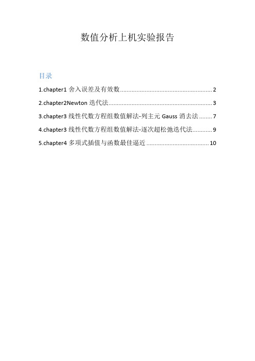
数值分析上机实验报告目录1.chapter1舍入误差及有效数 (2)2.chapter2Newton迭代法 (3)3.chapter3线性代数方程组数值解法-列主元Gauss消去法 (7)4.chapter3线性代数方程组数值解法-逐次超松弛迭代法 (9)5.chapter4多项式插值与函数最佳逼近 (10)1.chapter1舍入误差及有效数1.1题目设S N =∑1j 2−1N j=2,其精确值为)11123(21+--N N 。
(1)编制按从大到小的顺序11131121222-+⋯⋯+-+-=N S N ,计算S N 的通用程序。
(2)编制按从小到大的顺序1211)1(111222-+⋯⋯+--+-=N N S N ,计算S N 的通用程序。
(3)按两种顺序分别计算64210,10,10S S S ,并指出有效位数。
(编制程序时用单精度)(4)通过本次上机题,你明白了什么?1.2编写相应的matlab 程序clear;N=input('please input N:');AValue=((3/2-1/N-1/(N+1))/2);sn1=single(0);sn2=single(0);for i=2:Nsn1=sn1+1/(i*i-1); %从大到小相加的通用程序%endep1=abs(sn1-AValue);for j=N:-1:2sn2=sn2+1/(j*j-1); %从小到大相加的通用程序%endep2=abs(sn2-AValue);fprintf('精确值为:%f\n',AValue);fprintf('从大到小的顺序累加得sn=%f\n',sn1);fprintf('从大到小相加的误差ep1=%f\n',ep1);fprintf('从小到大的顺序累加得sn=%f\n',sn2);fprintf('从小到大相加的误差ep2=%f\n',ep2);disp('=================================');1.3matlab 运行程序结果>> chaper1please input N:100精确值为:0.740050从大到小的顺序累加得sn=0.740049从大到小相加的误差ep1=0.000001从小到大的顺序累加得sn=0.740050从小到大相加的误差ep2=0.000000>> chaper1please input N:10000精确值为:0.749900从大到小的顺序累加得sn=0.749852从大到小相加的误差ep1=0.000048从小到大的顺序累加得sn=0.749900从小到大相加的误差ep2=0.000000>> chaper1please input N:1000000精确值为:0.749999从大到小的顺序累加得sn=0.749852从大到小相加的误差ep1=0.000147从小到大的顺序累加得sn=0.749999从小到大相加的误差ep2=0.0000001.4结果分析以及感悟按照从大到小顺序相加的有效位数为:5,4,3。
数值分析大作业(利用MATLAB软件)

实验报告课程名称:数值分析实验项目:曲线拟合/数值积分专业班级:姓名:学号:实验室号:实验组号:实验时间:20.10.24 批阅时间:指导教师:成绩:工业大学实验报告(适用计算机程序设计类)专业班级:学号:姓名:实验名称:曲线拟合与函数插值附件A 工业大学实验报告(适用计算机程序设计类)专业班级:学号:姓名:实验步骤或程序:附录一:1.利用二次,三次,四次多项式进行拟合:1.1 MATLAB代码如下:clear;clc;close allt=[0 1 2 3 4 5 6 7 8 9 10 11 12 13 14 15 16 17 18 19 20 21 22 23 24];y=[14 13 13 13 13 14 15 17 19 21 22 24 27 30 31 30 28 26 24 23 21 19 17 16 15];%输入数据hold on[p2 s2]=polyfit(t,y,2);%对于上面的数据进行2次多项式拟合,其中s2包括R(系数矩阵的QR分解的上三角阵),%df(自由度),normr(拟合误差平方和的算术平方根)。
y2=polyval(p2,t);%返回多项式拟合曲线在t处的值[p3 s3]=polyfit(t,y,3);y3=polyval(p3,t);[p4 s4]=polyfit(t,y,4);y4=polyval(p4,t);plot(t,y,'ro')%画图plot(t,y2,'g-')plot(t,y3,'m^-')plot(t,y4,'bs-')xlabel('t')ylabel('y')legend('原始数据','2次多项式拟合','3次多项式拟合','4次多项式拟合')1.2 二次,三次,四次多项式拟合的结果分别如下:(1)总的拟合结果在工作区的显示如下:(2)其次二次多项式拟合的结果为:(3)其中三次多项式拟合的结果:(4)其中四次多项式拟合的结果为:1.3 拟合的图像为:1.4 拟合的多项式为:根据工作区得出的数据列出最后的拟合多项式为:(1)y=7.416+2.594t-0.094t^2(2)y=12.251-0.102t+0.193t^2-0.008t^3(3)y=15.604-3.526t+0.866t^2-0.052t^3+0.0009t^42.形如2()()b t c y t ae--=的函数,其中,,a b c 为待定常数。
——数值分析上机题

.......................课程名称:数值分析上机实习报告姓名:学号:专业:联系电话:目录序言 (3)第1章必做题 (4)1.1必做题第一题 (4)1.1.1题目 (4)1.1.2 分析 (4)1.1.3 计算结果 (4)1.1.3 总结 (6)1.2必做题第二题 (6)1.2.1题目 (6)1.2.2分析 (6)1.2.3计算结果 (6)1.2.4结论 (8)1.1必做题第一题....................................................................... 错误!未定义书签。
1.1.1题目 ............................................................................ 错误!未定义书签。
第2章选做题 (8)2.1选做题第一题 (8)2.1.1题目 (8)2.1.2分析 (8)2.1.3计算结果 (8)附录 (10)附录一:必做题第一题程序 (10)附录二:必做题第二题程序 (11)附录三:选做题第一题的程序 (13)序言本次数值分析上机实习采用Matlab数学软件。
Matlab是一种用于算法开发、数据可视化、数据分析以及数值计算的高级技术计算语言和交互式环境。
在数值分析应用中可以直接调用Matlab软件中已有的函数,同时用户也可以将自己编写的实用程序导入到Matlab函数库中方便自己调用。
基于Matlab数学软件的各种实用性功能与优点,本次数值分析实习决定采用其作为分析计算工具。
1.编程效率高MATLAB是一种面向科学与工程计算的高级语言,允许使用数学形式的语言编写程序,且比BASIC、FORTRAN和C等语言更加接近我们书写计算公式的思维方式,用MATLAB编写程序犹如在演算纸上排列出公式与求解问题。
因此,MATLAB语言也可通俗地称为演算纸式科学算法语言。
- 1、下载文档前请自行甄别文档内容的完整性,平台不提供额外的编辑、内容补充、找答案等附加服务。
- 2、"仅部分预览"的文档,不可在线预览部分如存在完整性等问题,可反馈申请退款(可完整预览的文档不适用该条件!)。
- 3、如文档侵犯您的权益,请联系客服反馈,我们会尽快为您处理(人工客服工作时间:9:00-18:30)。
2015.1.9
上机作业题报告
JONMMX 2000
1.Chapter 1
1.1题目
设S N =∑1j 2−1
N j=2
,其精确值为
)1
1
123(21+--N N 。
(1)编制按从大到小的顺序1
1
131121222-+
⋯⋯+-+-=N S N ,计算S N 的通用程序。
(2)编制按从小到大的顺序1
21
1)1(111222-+
⋯⋯+--+-=
N N S N ,计算S N 的通用程序。
(3)按两种顺序分别计算64210,10,10S S S ,并指出有效位数。
(编制程序时用单精度) (4)通过本次上机题,你明白了什么?
1.2程序
1.3运行结果
1.4结果分析
按从大到小的顺序,有效位数分别为:6,4,3。
按从小到大的顺序,有效位数分别为:5,6,6。
可以看出,不同的算法造成的误差限是不同的,好的算法可以让结果更加精确。
当采用从大到小的顺序累加的算法时,误差限随着N 的增大而增大,可见在累加的过程中,误差在放大,造成结果的误差较大。
因此,采取从小到大的顺序累加得到的结果更加精确。
2.Chapter 2
2.1题目
(1)给定初值0x 及容许误差ε,编制牛顿法解方程f(x)=0的通用程序。
(2)给定方程03
)(3
=-=x x
x f ,易知其有三个根3,0,3321=
*=*-=*x x x
○1由牛顿方法的局部收敛性可知存在,0>δ当),(0δδ+-∈x 时,Newton 迭代序列收敛于根x2*。
试确定尽可能大的δ。
○2试取若干初始值,观察当),1(),1,(),,(),,1(),1,(0+∞+-----∞∈δδδδx 时Newton 序列的收敛性以及收敛于哪一个根。
(3)通过本上机题,你明白了什么?
2.2程序
2.3运行结果
(1)寻找最大的δ值。
算法为:将初值x0在从0开始不断累加搜索精度eps,带入Newton迭代公式,直到求得的根不再收敛于0为止,此时的x0值即为最大的sigma值。
运行Find.m,得到在不同的搜索精度下的最大sigma值。
可见,在(−∞,−1)区间取初值,Newton序列收敛,且收敛于根−√3。
可见,在(−1,−δ)取初值,Newton序列收敛,且收敛于根√3。
可见,在(−δ,δ)取初值,Newton序列收敛,且收敛于根0。
可见,在(δ,1)取初值,Newton序列收敛,且收敛于根−√3
可见,在(1,+∞)取初值,Newton序列收敛,且收敛于根√3
3.Chapter 3
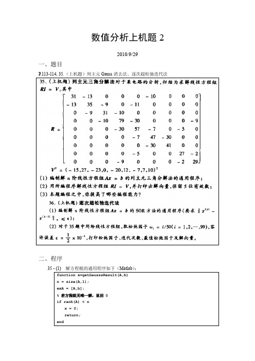
3.1题目
对于某电路的分析,归结为求解线性方程组RI=V,其中
31130
001000013359011000009311000000001079300009000305770500
0007473000000003041000
0005002720009000229R --⎛⎫ ⎪--- ⎪ ⎪-- ⎪--- ⎪ ⎪=--- ⎪
-- ⎪ ⎪- ⎪
-- ⎪ ⎪--⎝⎭
()15,27,23,0,20,12,7,7,10T
T V =----
(1)编制解n 阶线性方程组Ax =b 的列主元高斯消去法的通用程序;
(2)用所编程序线性方程组RI =V ,并打印出解向量,保留5位有效数字; (3)本题编程之中,你提高了哪些编程能力?
3.2程序
3.3运行结果
可看出,算得的该线性方程组的解向量为:
[-0.28923 0.34544 -0.71281 -0.22061 -0.4304 0.15431 -0.057823 0.20105 0.29023] 4.Chapter 4
4.1题目
(1)编制求第一型3次样条插值函数的通用程序;
(2)已知汽车门曲线型值点的数据如下:
端点条件为y010
S(i+0.5),i=0,1, (9)
4.2程序
4.3运行结果
5.Chapter 5
5.1题目
用Romberg求积法计算积分
∫
1
1+100x2
dx
1
−1的近似值,要求误差不超过0.5×10⁻⁷。
5.2程序
5.3运行结果
5.4结果分析
手动化简该定积分并最终求得的值为:0.0747,误差限为:3.486×10⁻⁸,可见,程序完成了计算要求。
6.Chapter 6
6.1题目
常微分方程初值问题数值解
(1)编制RK4方法的通用程序;
(2)编制AB4方法的通用程序(由RK4提供初值);
(3)编制AB4-AM4预测校正方法通用程序(由RK4提供初值);
(4)编制带改进的AB4-AM4预测校正方法通用程序(由RK4提供初值);
(5)对于初值问题
{y ′=−x 2y 2y (0)=3
取步长h=0.1,应用(1)-(4)中的四种方法进行计算,并将计算结果和精确解y (x )=3/(1+x 3)作比较;
(6)通过本上机题,你能得到哪些结论?
6.2程序
6.3运行结果(1)RK4法
6.4结果分析
从每一种方法的计算误差可以看出,精度由高到低依次是:RK4法、改进的AB4-AM4法、AB4-AM4法、AB4法。