General Equilibrium-notes-高微
北大高微讲义第2章 比较静态分析
p= p0
= - D33 D
15
2.1 斯拉茨基方程
(Slutsky equation)
1、利用最优决策的一阶条件:传统的推导方法
• 总结:由上面的推导可知
( 1 ) ∂ x1 = λ D11 + x1 D31
∂ p1
D
D
( 2)
∂ x1 ∂ p1
u =u0
=
λ D11 , D
L ( x1 , x 2 , µ ) = p1 x1 + p 2 x 2 + µ (u 0 − u ( x1 , x 2 ))
∂L
∂
x1
=
p1 − µ
∂u ∂ x1
=0
FOC :
∂L
∂
x
2
=
p2 − µ
∂u ∂x2
=0
∂L ∂µ
= u 0 − u ( x1 , x2 ) = 0
8
2.1 斯拉茨基方程
(Slutsky equation)
• 求总效应
∂ x1 ∂ p1
=
?
(从效用最大化出发)
max
u ( x1 , x2 )
s.t
p1 x1 + p 2 x2 = m
L ( x1 , x2 , λ ) = u ( x1 , x2 ) + λ (m − p1 x1 − p2 x2 )
FOC :
∂L
∂
=
−1
0
0
∂ p 1
运用克莱姆法则,可得
∂ x1 ∂ p1
= u = u 0
D11 µD
= λ D11 D
10
2.1 斯拉茨基方程
(Slutsky equation)
伦敦经济学院高微讲义-一般均衡
R2 b
Ob
R1b
x1 b
...as an Australian
x1 b R1b Ob
R2 b
x2 b
How BillBill's responds as p1/p2 changes... offer curve
x1
b
R1b
Ob
R2 b
x2 b
The twoconsistent offer curves Offers are only where curves Satisfies materials balance Price-taking utility-maximising Bill But, by construction... This is the competitive equilibrium Price-taking utility-maximising Alf b intersect R b 1 x b
Why price-taking?
General equilibrium
Robinson Crusoe’s problem
Decentralisation and Trade
A manyperson Economy
Why pricetaking?
Excess demand
An exchange economy
Microeconomics
General Equilibrium: price taking
Overview...
General Equilibrium
Robinson Crusoe's Problem
Decentralisation and Trade
白重恩-高级微观经济学讲义-Notes1-04

∴效用函数不是唯一的,u 和 f·u 是代表同样偏好的效用函数。 Divide the properties of utility function into two categories: (1) Ordinal properties: a property of U is ordinal if the property is also satisfied by any monotonically
Proof: with an additional condition:
X = Rn. is monotonic.
x ∈ Rn , x >> y ⇔ xi > yi ;
x ≥ y ⇔ xi ≥ yi.
m is monotonicity: if x >> y ⇒ x y. co is strong monotonicity: if x ≥ y & x ≠ y ⇒ x y.
中华经济学习网
2004 年秋季学期
高级微观经济学Ⅰ(讲义整理)
授课教授:白重恩
Ch1. 偏好和选择
一、消费者理论概述
选择消费品时,追求效用最大化(utility maximization),但同时要受收入的限制。
maxU (x1, x2 ) s.t. p1x1 + p2x2 ≤ w.
In summary, we have shown that ∀x, ∃a ∈ R, s.t. x ∼ ae.
Def: u(x) = a.
?
Prob: x y ⇒ u(x) ≥ u( y) .
高微文章job-market-signaling说课材料

University
Harvard University (Ph.D.) University of Oxford (B.A.) Princeton University (B.A.)
Contribution Signaling theory
Awards
John Bates Clark Medal (1981)
1. Introduction
What is the purpose of this essay ?
• analyze the phenomena of signaling which affect the market
• outline a model in which signaling is implicitly defined
NobБайду номын сангаасl Memorial Prize in Economics (2001) along with George
A. Akerlof and Joseph E. Stiglitz, for their market analyses in situation of
asymmetry of information
Content
1. Introduction 2. Hiring as an investment under uncertainty 3. Applicant signaling 4. Informational feedback and definition of equilibrium 5. Properties of informational equilibrium: an example 6. Informational impact of indices 7. Conclusion
伦敦经济学院高微讲义一般均衡
Resources Shares in firms
Net outputs Prices
Profits
Rents
let's look at the role of prices
And Nsoetporuoftpitustdsedpeepnedndononpprirciecse.s.....
y = y (p) f
Three major components
people's
These
teasntescaptsecuhlnaotleogy
almost all the steps
in resource sttohckes course so far
What is an economy?
Resources
n of R1 , R2 ,... these
n
P
f(p):=
S
i=1
pi
yif(p)
n
nf
S S Mh = pi Rih + Vfh P f(p)
i=1
f=1
Mh = Mh(p)
..S.aon, dtaskuienbtts.hot..iewhtuaohtlurleioecstceshhpaheitominlpodsnrpeirlcsaiee.ess.-s.pai:nocnoslmelese.c.t.rieolnatoifon
ownership rights of
everything on the island
So what does household h
possess?
Rih0
Resources
Shares in firms' profits
高级微观经济学(上海财经大学 陶佶)note02

Let x1 , x2 and x3 be any three consumption bundles in X .
Axiom 2.1 - Complete. Either x1 \ x2 or x2 \ x1 .
上海财大经济学院
2
作者:陶佶
2005 年秋季
高等微观经济学 I
Axiom 2.2 - Reflexive. For all x in X , x \ x . Axiom 2.3 - Transitive. If x1 \ x2 and x2 \ x3 , then x1 \ x3 .
Let X be a consumption set, a collection of all alternatives or complete consumption plans. The consumption set is also called as the choice set. Let xi ∈ be the number of units of ith
good, and x = ( x1, x2 , , xn ) be a vector containing different quantities of n commodities,
called as a consumption bundle or a consumption plan.
Properties of the Consumption Set, X : The minimal requirements are
Terminology 1. Let x0 be any points in the consumption set X . Relative to any such point,
高级微观经济学讲义

高级微观经济学讲义:均衡、福利与寻租理论主讲人:邢祖礼西南财经大学经济学院(2013秋季)一、教学目的与要求通过本讲,让学生了解局部均衡、一般均衡的基本思想,掌握帕累托最优、超额需求函数、经济核等重要概念,熟悉福利经济学第一定理、第二定理、核定理,能够较为详细的理解均衡的存在性问题。
二、基本内容与课时安排1、局部均衡(3课时)2、交换均衡:求解(3课时)3、生产均衡(3课时)4、寻租与中国经济增长的特征(3课时)共计:12课时(2周)三、参考书目杰弗瑞.杰里菲利普.瑞尼:《高级微观经济学》,上海财经大学出版社2002年。
Andreu Mas-Colell Michael D.Whinston and Jerry R.Green:“Microeconomic Theory”,上海财经大学出版社2005年。
附:讲义的基本内容高级微观经济学讲义:均衡、福利与寻租理论邢祖礼西南财经大学经济学院2013年秋季第一讲:局部均衡分析一、竞争性均衡1、拟线性效用函数Quasi-linear utility function:)(),(i i i i i i x m x m u ϕ+=, i x 是一个消费产品, i m 是其他所产品的支出。
这种函数形式暗含两个假设:(1) x 产品没有收入效应,即x 产品的边际效用独立于收入m ;(2) x 产品的价格不影响其他产品的价格。
通过这两个假设,我们可以得出:其他产品的价格独立于x 产品。
2、需求:)(max i i i x m ϕ+s.t. i i i m p x y +⋅≤ (*)从 (*)中, 我们有:i i i m y p x =-⋅代入目标函数有:max ()ii i i i x x p x y φ-⋅+*()i i x p ϕ'=。
需求量 *i x 依赖于 p 并随着 p 变化. *i x 独立于收入;市场需求∑==Ii i p x p X 1*)()(, 它独立于禀赋分配和产权。
哈佛大学MILLER教授为MWG写的高微笔记 (1)
Notes on Microeconomic TheoryNolan lerAugust18,2006Contents1The Economic Approach12Consumer Theory Basics52.1Commodities and Budget Sets (5)2.2Demand Functions (8)2.3Three Restrictions on Consumer Choices (9)2.4A First Analysis of Consumer Choices (10)2.4.1Comparative Statics (11)2.5Requirement1Revisited:Walras’Law (11)2.5.1What’s the Funny Equals Sign All About? (12)2.5.2Back to Walras’Law:Choice Response to a Change in Wealth (13)2.5.3Testable Implications (14)2.5.4Summary:How Did We Get Where We Are? (15)2.5.5Walras’Law:Choice Response to a Change in Price (15)2.5.6Comparative Statics in Terms of Elasticities (16)2.5.7Why Bother? (17)2.5.8Walras’Law and Changes in Wealth:Elasticity Form (18)2.6Requirement2Revisited:Demand is Homogeneous of Degree Zero (18)2.6.1Comparative Statics of Homogeneity of Degree Zero (19)2.6.2A Mathematical Aside (21)2.7Requirement3Revisited:The Weak Axiom of Revealed Preference (22)2.7.1Compensated Changes and the Slutsky Equation (23)2.7.2Other Properties of the Substitution Matrix (27)3The Traditional Approach to Consumer Theory293.1Basics of Preference Relations (30)3.2From Preferences to Utility (35)3.2.1Utility is an Ordinal Concept (36)3.2.2Some Basic Properties of Utility Functions (37)3.3The Utility Maximization Problem(UMP) (42)3.3.1Walrasian Demand Functions and Their Properties (47)3.3.2The Lagrange Multiplier (49)3.3.3The Indirect Utility Function and Its Properties (50)3.3.4Roy’s Identity (52)3.3.5The Indirect Utility Function and Welfare Evaluation (54)3.4The Expenditure Minimization Problem(EMP) (55)3.4.1A First Note on Duality (57)3.4.2Properties of the Hicksian Demand Functions and Expenditure Function (59)3.4.3The Relationship Between the Expenditure Function and Hicksian Demand.623.4.4The Slutsky Equation (65)3.4.5Graphical Relationship of the Walrasian and Hicksian Demand Functions..673.4.6The EMP and the UMP:Summary of Relationships (71)3.4.7Welfare Evaluation (72)3.4.8Bringing It All Together (78)3.4.9Welfare Evaluation for an Arbitrary Price Change (83)4Topics in Consumer Theory874.1Homothetic and Quasilinear Utility Functions (87)4.2Aggregation (89)4.2.1The Gorman Form (90)4.2.2Aggregate Demand and Aggregate Wealth (92)4.2.3Does individual W ARP imply aggregate WARP? (94)4.2.4Representative Consumers (96)4.3The Composite Commodity Theorem (98)4.4So Were They Just Lying to Me When I Studied Intermediate Micro? (99)4.5Consumption With Endowments (101)4.5.1The Labor-Leisure Choice (104)4.5.2Consumption with Endowments:A Simple Separation Theorem (106)4.6Consumption Over Time (110)4.6.1Discounting and Present Value (111)4.6.2The Two-Period Model (112)4.6.3The Many-Period Model and Time Preference (115)4.6.4The Fisher Separation Theorem (118)5Producer Theory1215.1Production Sets (122)5.1.1Properties of Production Sets (123)5.1.2Profit Maximization with Production Sets (127)5.1.3Properties of the Net Supply and Profit Functions (129)5.1.4A Note on Recoverability (132)5.2Production with a Single Output (133)5.2.1Profit Maximization with a Single Output (134)5.3Cost Minimization (136)5.3.1Properties of the Conditional Factor Demand and Cost Functions (138)5.3.2Return to Recoverability (139)5.4Why Do You Keep Doing This to Me? (140)5.5The Geometry of Cost Functions (141)5.6Aggregation of Supply (142)5.7A First Crack at the Welfare Theorems (143)5.8Constant Returns Technologies (144)5.9Household Production Models (148)5.9.1Agricultural Household Models with Complete Markets (149)6Choice Under Uncertainty1586.1Lotteries (160)6.1.1Preferences Over Lotteries (161)6.1.2The Expected Utility Theorem (164)6.1.3Constructing a vNM utility function (167)6.2Utility for Money and Risk Aversion (168)6.2.1Measuring Risk Aversion:Coefficients of Absolute and Relative Risk Aversion1736.2.2Comparing Risk Aversion (174)6.2.3A Note on Comparing Distributions:Stochastic Dominance (176)6.3Some Applications (178)6.3.1Insurance (178)6.3.2Investing in a Risky Asset:The Portfolio Problem (180)6.4Ex Ante vs.Ex Post Risk Management (182)7Competitive Markets and Partial Equilibrium Analysis1857.1Competitive Equilibrium (186)7.1.1Allocations and Pareto Optimality (186)7.1.2Competitive Equilibria (188)7.2Partial Equilibrium Analysis (191)7.2.1Set-Up of the Quasilinear Model (191)7.2.2Analysis of the Quasilinear Model (192)7.2.3A Bit on Social Cost and Benefit (195)7.2.4Comparative Statics (195)7.3The Fundamental Welfare Theorems (198)7.3.1Welfare Analysis and Partial Equilibrium (201)7.4Entry and Long-Run Competitive Equilibrium (205)7.4.1Long-Run Competitive Equilibrium (206)7.4.2Final Comments on Partial Equilibrium (209)8Externalities and Public Goods2118.1What is an Externality? (211)8.2Bilateral Externalities (213)8.2.1Traditional Solutions to the Externality Problem (217)8.2.2Bargaining and Enforceable Property Rights:Coase’s Theorem (219)8.2.3Externalities and Missing Markets (221)8.3Public Goods and Pure Public Goods (222)8.3.1Pure Public Goods (223)8.3.2Remedies for the Free-Rider Problem (227)8.3.3Club Goods (229)8.4Common-Pool Resources (229)9Monopoly2339.1Simple Monopoly Pricing (233)9.2Non-Simple Pricing (236)9.2.1Non-Linear Pricing (237)9.2.2Two-Part Tariffs (239)9.3Price Discrimination (241)9.3.1First-Degree Price Discrimination (241)9.3.2Second-Degree Price Discrimination (243)9.3.3Third-Degree Price Discrimination (247)9.4Natural Monopoly and Ramsey Pricing (249)9.4.1Regulation and Incentives (251)9.5Further Topics in Monopoly Pricing (252)9.5.1Multi-Product Monopoly (252)9.5.2Intertemporal Pricing (255)9.5.3Durable Goods Monopoly (256)These notes are intended for use in courses in microeconomic theory taught at Harvard Univer-sity.Consequently,much of the structure is inherited from the required text for the course,which is currently Mas-Colell,Whinston,and Green’s Microeconomic Theory(referred to as MWG in these notes).They also draw on material contained in Silberberg’s The Structure of Economics,as well as additional sources.They are not intended to stand alone or in any way replace the texts.In the early drafts of this document,there will undoubtedly be mistakes.I welcome comments from students regarding typographical errors,just-plain errors,or other comments on how these notes can be made more helpful.I thank Chris Avery,Lori Snyder,and Ben Sommers for helping clarify these notes andfinding many errors.Chapter1The Economic ApproachEconomics is a social science.1Social sciences are concerned with the study of human behavior. If you asked the next person you meet while walking down the street what defines the difference between economics and other social sciences,such as political science or sociology,that person would most likely say that economics studies money,interest rates,prices,profits,and the like, while political science considers politicians,elections,etc.,and sociology studies the behavior of groups of people.However,while there is certainly some truth to this statement,the things that can be fairly called economics are not so much defined by a subject matter as they are united by a common approach to problems.In fact,economists have written on topics spanning human behavior,from traditional studies offirm and consumer behavior,interest rates,inflation and unemployment to less traditional topics such as social choice,voting,marriage,and family.The feature that unites these studies is a common approach to problems,which has become known as the“marginalist”or“neoclassical”approach.In a nutshell,the marginalist approach consists of four principles:1.Economic actors have preferences over allocations of the world’s resources.These preferencesremain stable,at least over the period of time under study.22.There are constraints placed on the allocations that a person can achieve by such things aswealth,physical availability,and social/political institutions.3.Given the limits in(2),people choose the allocation that they most prefer.1See Silberberg’s Structure of Economics for a more extended discussion along these lines.2Often preferences that change can be captured by adding another attribute to the description of an allocation. More on this later.4.Changes in the allocations people choose are due to changes in the limits on available resourcesin(2).The marginalist approach to problems allows the economist to derive predictions about behavior which can then,in principle,be tested against real world data using statistical(econometric) techniques.For example,consider the problem of what I should buy when I go to the grocery store.The grocery store isfilled with different types of food,some of which I like more and some of which I like less.Principle(1)says that the trade-offs I am willing to make among the various items in the store are well-defined and stable,at least over the course of a few months.An allocation is all of the stuffthat I decide to buy.The constraints(2)put on the allocations I can buy include the stock of the items in the store(I can’t buy more bananas than they have)and the money in my pocket(I can’t buy bananas I can’t afford).Principle(3)says that given my preferences,the amount of money in my pocket and the stock of items in the store,I choose the shopping cart full of stuffthat I most prefer.That is,when I walk out of the store,there is no other shopping cart full of stuffthat I could have purchased that I would have preferred to the one I did purchase. Principle(4)says that if next week I buy a different cart full of groceries,it is because either I have less money,something I bought last week wasn’t available this week,or something I bought this week wasn’t available last week.There are two natural objections to the story I told in the last paragraph,both of which point toward why doing economics isn’t a trivial exercise.First,it is not necessarily the case that my preferences remain stable.In particular,it is reasonable to think that my preferences this week will depend on what I purchased last week.For example,if I purchased chocolate chip cookies last week,this may make me less likely to purchase them this week and more likely to purchase some other sort of cookie.Thus,preferences may not be stable over the time period we are studying.Economists deal with this problem in two ways.Thefirst is by ignoring it.Although widely applied,this is not the best way to address the problem.However,there are circumstances where it is reasonable.Many times changes in preferences will not be important relative to the phenomenon we are studying.In this case it may be more trouble than it’s worth to address these problems.The second way to address the problem is to build into our model of preferences the idea that what I consumed last week may affect my preferences over what I consume this week. In other words,the way to deal with the cookie problem is to define an allocation as“everything I bought this week and everything I bought last week.”Seen in this light,as long as the effect of having chocolate chip cookies last week on my preferences this week stay stable over time,mypreferences stay stable,whether or not I actually had chocolate chip cookies last week.Hence if we define the notion of preferences over a rich enough set of allocations,we can usuallyfind preferences that are stable.The second problem with the four-step marginalist approach outlined above is more trouble-some:Based on these four steps,you really can’t say anything about what is going to happen in the world.Merely knowing that I optimize with respect to stable preferences over the groceries I buy,and that any changes in what I buy are due to changes in the constraints I face does not tell me anything about what I will buy,what I should buy,or whether what I buy is consistent with this type of behavior.The solution to this problem is to impose structure on my preferences.For example,two common assumptions are to assume that I prefer more of an item to less3(monotonicity)and that I spend my entire grocery budget in the store(Walras’Law).Another common assumption is that only real opportunities matter.If I were to double all of the prices in the store and my grocery budget,this would not affect what I can buy,so it shouldn’t affect what I do buy.Once I have added this structure to my preferences,I am able to start to make predictions about how I will behave in response to changes in the environment.For example,if my grocery budget were to increase,I would buy more of at least one item(since I spend all of my money and there is always some good that I would like to add to my grocery cart).4This is known as a testable implication of the theory.It is an implication because if the theory is true,I should react to an increase in my budget by buying more of some good.It is testable because it is based on things which are,at least in principle,observable.For example,if you knew that I had walked into the grocery store with more money than last week and that the prices of the items in the store had not changed,and yet I left the store with less of every item than I did last week,something must be wrong with the theory.Thefinal step in economic analysis is to evaluate the tests of the theories,and,if necessary, change them.We assume that people follow steps1-4above,and we impose restrictions that we believe are reasonable on their preferences.Based on this,we derive(usually using math)predic-tions about how they should behave and formulate testable hypotheses(or refutable propositions) about how they should behave if the theory is true.Then we observe what they really do.If 3Or,we could make the weaker assumption that no matter what I have in my cart already,there is something in the store that I would like to add to my cart if I could.4The process of deriving what happens to people’s choices(the stuffin the cart)in response to changes in things they do not choose(the money available to spend in the store)is known as comparative statics.Nolan Miller Notes on Microeconomic Theory:Chapter1ver:Aug.2006their behavior accords with our predictions,we rejoice because the real world has supported(but not proven!)our theory.If their behavior does not accord with our predictions,we go back to the drawing board.Why didn’t their behavior accord with our predictions?Was it because their preferences weren’t like we though they were?Was it because they weren’t optimizing?Was it because there was an additional constraint that we didn’t understand?Was it because we did not account for a change in the environment that had an important effect on people’s behavior?Thus economics can be summarized as follows:It is the social science that attempts to account for human behavior as arising from consistent(often maximizing—more on that later)behavior subject to one or more constraints.Changes in behavior are attributed to changes in the con-straints,and the test of these theories is to compare the changes in behavior predicted by the theory with the changes that actually occur.4。
高级微观经济学讲义:均衡与福利
高级微观经济学讲义:平衡与福利主讲人:邢祖礼西南财经大学经济学院〔2021秋季〕一、教学目的与要求通过本讲,让学生理解部分平衡、一般平衡的根本思想,掌握帕累托最优、超额需求函数、经济核等重要概念,熟悉福利经济学第一定理、第二定理、核定理,可以较为详细的理解平衡的存在性问题。
二、根本内容与课时安排1、部分平衡〔3课时〕2、交换平衡:求解〔2课时〕3、消费:求解克鲁索经济〔2课时〕4、平衡的存在性〔1课时〕5、核与核定理〔2课时〕6、答疑与作业讲解〔2课时〕共计:12课时〔两周〕三、参考书目杰弗瑞.杰里菲利普.瑞尼:?高级微观经济学?,上海财经大学出版社2002年。
:“Microeconomic Theory〞,上海财经大学出版社2005年。
附:讲义的根本内容高级微观经济学讲义:平衡与福利邢祖礼西南财经大学经济学院2021年秋季第一讲:部分平衡分析一、竞争性平衡1、拟线性效用函数Quasi-linear utility function:)(),(i i i i i i x m x m u ϕ+=, i x 是一个消费产品, i m 是其他所产品的支出。
这种函数形式暗含两个假设:(1) x 产品没有收入效应,即x 产品的边际效用独立于收入m ;(2) x 产品的价格不影响其他产品的价格。
通过这两个假设,我们可以得出:其他产品的价格独立于x 产品。
2、需求:)(max i i i x m ϕ+s.t. ∑=-⋅+≤⋅+Jj j j j ij i i i q C q p x p m 1)]([θω (*)从 (*)中, 我们有:i Jj j j j ij i i x p q C q p m ⋅--⋅+=∑=1)]([θω代入目的函数有:∑=-⋅++⋅-Jj j j j ij i i i i x q C q p x p x i1)]([)(max θωϕ0)0(*=⇒≤'i i x p ϕ*()i i x p ϕ'=。
微观经济学教材推荐
经济学 专业 必读书目
一、入门教材:
1、曼昆《经济学原理》上下册,88元。梁小民教授翻译。曼昆为哈佛高才生,天才横溢,属新古典凯恩斯主义学派,研究范围偏重宏观经济分析。 该书为大学一年级学生而写,主要特点是行文简单、说理浅显、语言有趣。界面相当友好,引用大量的案例和报刊文摘,与生活极其贴近,诸如美联储为何存在,如何运作,Greenspan 如何降息以应付经济低迷等措施背后的经济学道理。该书几乎没有用到数学,而且自创归纳出“经济学10大原理”,为初学者解说,极其便利完全没有接触过经济学的人阅读。学此书,可了解经济学的基本思维,常用的基本原理,用于看待生活中的经济现象。可知经济学之功用及有趣,远超一般想象之外。推荐入门首选阅读。目前国内已经有某些教授依据此书编著《西方经济学》教材,在书中出现“经济学10大原理”一词,一眼便可看出是抄袭而来。
金庸小说与梁羽生小说恰恰相反,往往开头平淡中孕育玄机,随着情节逐步展开,人物越来越多,故事越来越纷纭复杂,但又环环入扣,引人入胜,如同烧一壶水,火越来越旺,水越来越沸腾。mas-colell,whiston,green合著的<微观经济学〉就深得其趣。全书结构博大雄浑,几乎涉及到了微观经济学的各个大小领域,但其结构安排井然有序,娓娓道来,绝对不失散乱。开篇高屋建瓴,给出了消费者理论的两种研究方法,选择法与偏好法同等对待,并行不悖,详细的论述了两种方法个中联系,逐步添加假设,以得出更深层次之结论,让读者对各假设与定义之来龙去脉了然于胸,而不仅是概念之堆积(varian之偏好假设部分似有此嫌)。这部分的特色还在于作出了总需求的推导,并分析了个人需求叠加为总需求后需求函数性质保留问题,让读者心安理得。此书厂商理论虽仍有其特色,终究失之薄弱。这也是一般高级微观通病,消费者理论先述,厂商理论与之相似处,尽量都省去。(但不知怎的,这本书连替代弹性这类定义也付之阙如,幸好varian的高级微观是厂商理论打头,至为详备,可以参考)。紧接着赶在均衡理论之前叙述博弈论,作为后面分析的工具之一,然后是局部均衡理论和市场失灵理论。第二册一开始,就进入了全书的高潮阶段:一般均衡,这的确是全书的精华之处,正如〈天龙八部〉第五册开篇的少林寺之会一样,几乎所有重要人物都在此先后登场,故事波澜壮阔,情节诡秘怪谲,在此书一般均衡的阐述中,几乎所有前述重要理论都在此重新出现,各显神通,层层递进,作出一个又一个假设,得出一个又一个结论,让人当叹鬼斧神工,叹为观止。在“均衡与时间”章,动态规划、索洛模型也杀将进来,加入消费者理论、生产者理论、博弈论、不确定性理论之战团,让人惊叹宏观乎?微观乎?当真是汪洋恣肆,横无际涯!紧接高潮之后,作者运用一般均衡理论,对社会福利与社会选择作出了分析。全书在个人需求的分析中开始,在全社会的福利分析中结束。
高微文章job-market-signaling教学提纲

asymmetry of information
Content
1. Introduction 2. Hiring as an investment under uncertainty 3. Applicant signaling 4. Informational feedback and definition of equilibrium 5. Properties of informational equilibrium: an example 6. Informational impact of indices 7. Conclusion
Field
Microeconomics Market analysis
University
Harvard University (Ph.D.) University of Oxford (B.A.) Princeton University (B.A.)
Contribution Signaling theory
Awards
John Bates Clark Medal (1981)
Nobel Memorial Prize in Economics (2001) along with George
A. Akerlof and Joseph E. Stiglitz, for their market analyses in situation of
Signaling case 1
2-y*/2
No-signaling case q1+2(1-q1)=2-q1
Signaling equilibrium in which group II is better off than no-signaling :
高级微观经济学教案-精选

理性经济人是平等化的个人。 (4)经济人理性的体现: 选择的一致性或偏好的可传递性;
理性意为有原因的、可推理的、可理解 的;
理性是指节约的、可计算的
理性表示合理的,假定人的行为总是一 种理性的审慎,即在众多可选择的方案 中,审慎的选择达到目标的最好的手段 或方法。因此,理性并非目的或手段, 而是指手段与目的的关系。
用理性理解自然,用理性理解社会,用理性 理解人
(4)近代科学方法
牛顿的物理学,找到了可以统一解释地球上 的机械运行和天体运动的万有引力,统一解 释了过去被看成不同物理现象的各种现象。 那么在人的世界中也应存在类似的内在动力。
斯密:同情心是人们伦理的第一动力; 利己心是人们的经济动力。
四、理智主义决定论
这种思维方式认为,应主要研究感观经 验后面的静止的、理智的、本质的、必 然的逻辑世界,从而为预测和解释可以 感知的世界提高某种基础观念。
经济学追求的是一个静止的、本质的、 具有支配性的理性世界。如均衡
经济学所研究的是一个具有逻辑性的、 必然性的、有严格秩序的理想世界。
人性恶
马基雅弗利:世界上存在一个统一的、 普遍的、永恒不变的人性,即自私或利 己的本性,支配人的行为的是自己的情 欲。
霍布斯把人看作是贪婪、恐惧、贪图享 乐的动物。
(2)个人主义 西方人文主义传统,以人权挑战神权
霍布斯的个人主义思想,以孤立的个人分析 社会
(3)理性主义传统
第一章 技术
对技术的描述最简单、最普通的方法是 生产函数,这里介绍一些更一般化的方 法。
1、生产集
假设有L种物品的经济。
生产向量(也称投入-产出向量或净产 出向量或生产计划)是一个向量
高级微观经济学讲义(清华 白重恩) Notes7-04
2004 年秋季
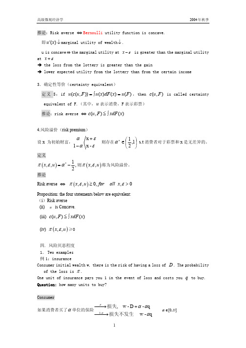
推论:Risk averse ⇔ Bernoulli utility function is concave. 即 u ′( x) ↓ marginal utility of wealth ↓ . u is concave ⇒ the marginal utility at x − ε is greater than the marginal utility at x + ε Î the loss from the lottery is greater than the gain Î lower expected utility from the lottery than from the certain income 3.确定性等价(certainty equivalent) 定 义 5 : if u (c(u , F )) = ∫ u ( x) dF ( x) = u ( F ) , then c(u , F ) is called certainty equivalent of F.(其中, u 表示消费,F 表示彩票) 推论:risk averse ⇔ c(u , F ) ≤ ∫ xdF ( x)
2
1 1 CE ( z ) = mz − ασ z2 , ασ z2 is risk premium. 2 2
Proposition:the 4 statement below are equivalent: (i) rA ( x, u 2 ) ≥ rA ( x, u1 ) for all x; (ii) u 2 ( x ) =
⇒−
χ ′′ u′ ≥ 0 χ′ 1
⇒ χ ′′ < 0
χ is a concave function
伦敦经济学院高微讲义-消费者理论(2)
The ordering of points is identical for each plane
0
Example for Independence Axiom
Red A A' 1 2
Blue 6 3
Green 10 10
The independence axiom
One and only one state-of-the-world can occur. So if the payoff in one state is fixed... the level at which the payoff is fixed should have no bearing on the orderings over prospects whose payoffs can differ in other states of the world
The Basics (Again)
The Consumer
Opportunities and Preferences
Optimisation and Comp. Statics
Welfare
Aggregation
Modelling Uncertainty
Expected Utility
Risk Aversion
Expected Utility
Risk Aversion
For more results we need more structure
Three extra axioms to clarify the consumer's attitude to uncertain prospects
Further restrictions on the structure of utility functions
白重恩-高级微观经济学讲义-Notes3-04
中
华
∂u ∂x i p = i for all General n:FOC 为 ∂u pj ∂x j
经
这就是边际替代率 MRS
——UMP 的一阶条件(first-order condition)FOC
济
∂u ∂u dx 2 + . =0 ∂x1 ∂x 2 dx1
学
If u is monotonic and strictly quasi-concave, then the solution of the FOC’s is the maximum of the utility function. Denote the solution by x( p, m) , Walrasian Demand Function.
.1 0
6
0j in g
In this case, x1 > 0, x2 = 0 . The indifference curve is steeper than the budget line.
ji .
官方总站
co m
中华经济学习网
中华经济学习网
2004 年秋季
Ch3. Classical Demand Theory
周海欧 江财高微讲义 4 一般均衡
《高级微观经济学》讲义江西财经大学周海欧副教授4General Equilibrium亚当·斯密提出的看不见的手的观点,构成了现代经济学的核心思想。
该观点认为,在自由竞争的市场环境下,理性的经济人基于自身利益最大化而做出的关于资源使用的分散决策,最终会导致一个在某种意义上而言符合全社会利益的合理结果。
Hayek: 自发的秩序引发了很多问题:(1)如何刻画理性经济人自身利益最大化的决策?(2)如何定义竞争性市场,其中人们的行动是如何互影响的?(3)什么是资源配置的社会最优标准?(4)完全竞争市场中人们的行为是否会使资源配置向某种特定的状态变动?(5)这种状态下资源配置是否符合社会最优标准?(6)这种状态是唯一的还是有着各种可能?(7)当经济从这种状态偏离时,能否自动回归?我们之前主要处理了(1),部分涉及(2)、(3)。
本讲将更深入地探讨(4)、(5)。
问题(6)、(7)暂不讨论。
4.1Barter Exchange economy (纯消费者物物交换经济)在考虑竞争性市场之前,我们先考虑一个简单的物物交换模型。
模型设定:纯消费者,无生产;每个人都是理性和自利的;每个人有一个初始商品束(禀赋);没有价格信号,只有物物交换;每个人都知道其他所有人的偏好和禀赋。
这个模型除了没有考虑生产,提供了一个近乎完美的世界:私有产权(所有资源属于私人)、自由交换(除了自愿交换没有任何其他途径来改变资源的使用权)、完全信息(每个人都掌握经济系统中的一切信息)。
协调机制方面,假定人们可以进行自由的组合,结成各种贸易联盟(Coalition),直到达成自己认为最满意的交易结果。
因此,在这样的模型世界中所形成的关于资源配置的结果,可以被看作是一种理想的资源配置。
弄清楚这样的经济中会出现什么样的结果,可以为我们了解竞争性市场的功能提供参考。
在这个模型中,资源配置是指所有商品在人群中分配的一个完整方案,是所有人的最终消费计划的一个完整列表。
高等代数教学中从低维到高维的思考和实践

高等代数教学中从低维到高维的思考和实践李小朝【摘要】Taking the analysis on the characteristics of the higher algebra course as a starting point,combined with the actual level of students in local colleges,analyzed the teaching of taking the low dimensional as examples to analyze the rules of solving problem,then summarizing the high dimensional situation,provide general conclusion through the multimedia teaching model.With this teaching methodology,students not only can understand the teaching content, but also can learn to analyze their own problems,thus obtained better teaching results.%从分析高等代数课程特点出发,结合地方高校学生实际水平,采取低维实例入手,分析解题规律,进而对高维情形进行概括和总结,并利用多媒体给出一般结论模式进行教学。
通过这种教学模式,学生理解了教学内容,更学会自己分析问题,取得较好的教学效果。
【期刊名称】《高师理科学刊》【年(卷),期】2015(000)010【总页数】4页(P69-71,75)【关键词】高等代数;低维;高维;教学模式【作者】李小朝【作者单位】黄淮学院数学科学系,河南驻马店 463000【正文语种】中文【中图分类】O15;G642.0高等代数是大学数学专业最重要的一门专业基础课,很多理论和方法对后续课程的学习非常重要.由于高等代数相对抽象,逻辑概括性强,使很多学生学起来感到比较吃力.高等代数中许多概念,定理是对一般维度n来给出,这样固然使概念结论比较严密,适应性广泛,但无疑也显得相对抽象,不好理解.一些学者从实际问题或者例子出发,给出了高等代数的教学模式[1-3].还有许多教育工作者对高等代数给出很多较好的学习或教学方法[4-7].但是对于地方本科院校,学生数学基础相对薄弱,教学更应从学生的实际水平出发,逐步提高.本文结合教材[8]和自身教学经验,对抽象概念和结论采取从低维实例入手,分析解题规律,进而对高维情形进行概括和总结,并利用多媒体给出一般结论模式进行教学.这样学生既理解了概念结论,又学会自己从低维入手分析问题,形成较好的学习习惯,从而也取得了较好的教学效果.1.1 行列式的概念n级行列式等于所有取自不同行不同列的n个元素乘积a1j1a2 j 2…anj n的代数和,这里j1j2…jn是1, 2, …, n的一个排列,每一项都按下面规则带有符号;当j1j2…jn是偶排列时,带有正号,当j1j2…jn是奇排列时,带有负号.这一定义可写成这里表示对所有n级排列求和.行列式这一章本来是相对简单的,可是很多学生尽管会计算,但是对定义的本身理解不很透彻.可以尝试从低维入手进行行列式概念的讲解.己分析n=3的情形,总结规律.最后教师分析一般规律,利用多媒体给出一般形式即可.1.2 线性空间的概念线性空间的概念在高等代数中非常重要,理论也很严谨深刻,但是同时也比较抽象,一些学生感到无从入手.线性空间的概念不再累述,详见文献[8].简言之就是非空集合V与数域P上定义2种运算,满足8条运算规律.其后在n维线性空间研究维数、基、坐标等.这里的研究不是针对某个具体对象,概括性很强,适用面很广,使一些学生感到“摸不着,看不到”,也就有无从下手之感.教学中也可采取从低维实例入手,高维概括总结的方式解决.首先分析数域P上集合V={( a, b)| a, b∈ P}.在V上有加法运算和P与V之间数乘运算,即(a1, b1)+( a2, b2)=( a1+ a2, b1+ b2),k( a, b)=( ka, kb).列出运算满足的规律,详见文献[8]第三章第二节.V中向量ε1=(1, 0),ε2=(0, 1)起着极大线性无关组的作用,即ε1, ε2线性无关,且V中任一向量都可由ε1, ε2线性表出.这里可以引出线性空间基和维数的概念,比较容易理解.然后分析数域P上多项式组成的集合V={次数小于3的多项式f( x)和零多项式}.在V上有加法运算,P与V之间数乘运算以及它们满足的运算规律可详见文献[8]第一章第二节.V中也有向量f1( x)=1,f2(x)=x,f3(x)=x2起着极大无关组的作用,即1, x, x2线性无关,且V中任一向量都可由1, x, x2线性表出.给出数域P上二级矩阵全体组成的集合.让学生根据第四章所学矩阵的运算,总结相关的运算规律和结论.最后,教师把这些不同的研究对象所具有的共同规律概括总结出来,也就是线性空间中的概念和性质,并通过多媒体展示.例1设A, B是数域P上的n级方阵,则这个定理在矩阵理论中非常实用,可能都习以为常了,但是它的证明过程有必要让学生理解清楚.教材中的证明是对一般量n来证明的,证明过程比较复杂枯燥.教学中可以尝试从低维情形入手,先把证明的思路和过程整理清楚.对一般的情形,有相同的推导过程,用多媒体给以演示证明.这样学生对定理证明的思路会比较清晰,运用结论也更得心应手.对于二级方阵A在黑板上讲解清楚之后,采用相同的思路分析问题,利用多媒体给出完整的证明.这样既能把问题分析清楚,又能加深印象,并且节约讲授时间.高等代数的许多习题都比较典型,也较复杂,需要认真分析.一些学生看着习题,总感到无从下手,缺少思路.其实习题也是一样,也可以从低维分析入手,寻找分析问题的思路和方法,然后高维概括总结,给出完整证明过程.分析过程对s=3已经完成证明,对一般s需要进一步分析.若不是直和,则有不全为零的i∈Viα(i =1, 2, …,s ),且0=α1+α2+…+αs.设αk是αs, αs-1, …,α2,α1中第1个不为零的向量,则有k≥2,且0,与已知矛盾,故可证结论成立.从低维实例入手,分析解题规律,高维概括总结,多媒体讲解一般结论.看似非常简单的教学模式,但是对地方高校数学专业的学生还是很实用的.这样学生既理解了高等代数的内涵,更学会了分析抽象问题的方法,养成自主学习的习惯,提高了分析问题和解决问题的能力.【相关文献】[1]冯克勤.高校代数教学的一些实践与思考[J].高等数学研究,2006(4):2-5[2]李尚志.从问题出发引入线性代数概念[J].高等数学研究,2006(5):6-9[3]梁建秀.实际问题驱动下的高等代数课程教学的实践探索[J].洛阳师范学院学报,2015(2):127-130[4]刘桂荣,闫卫平.提高高等代数教学质量的策略探讨[J].教育理论与实践,2012(30):44-46[5]刘小川,何美.高等代数教学方法的探讨[J].大学数学,2013(1):149-151[6]孙敏.高等代数课程教改的思考和实践[J].数学教育学报,2010(3):100-102[7]李小朝,邓伟娜.线性方程组在线性代数教学中的应用[J].高师理科学刊,2012,32(5):89-91[8]北京大学数学系.高等代数[M].4版.北京:高等教育出版社,2013,2013。
高级微观经济学market as a process

• Proof: Liaponov function: V(p) [(pipi)2]
dV(p)
dt
2(pipi)pi(t)2
(pipi)zi(p)
2 (pizi(p)pizi(p))0piz(p)0
Welfare
• Pareto criterion: x % x if and only if x % i x
See the fig.
The “core”
• Walrasian equilibrium is in core.
– Proof: let (x,p) be the Walrasian equilibrium
with initial endowment wi.
– If not , there is some coalition S and some
Tw A (V T )[w A wB ]
Vw A (V T )wB
• So the coalition with V agents of type A
and (V-T) of type B can improve upon y.
The “core”
• Convexity and size: • If agent has non-convex preference, is
• Compensation criterion (Kaldor ~):
x % x if there is x such that xi xi
and x % i x
Assignment
Core of an economy
Core
Pareto set
Endowment
Shrinking core
The “core”
- 1、下载文档前请自行甄别文档内容的完整性,平台不提供额外的编辑、内容补充、找答案等附加服务。
- 2、"仅部分预览"的文档,不可在线预览部分如存在完整性等问题,可反馈申请退款(可完整预览的文档不适用该条件!)。
- 3、如文档侵犯您的权益,请联系客服反馈,我们会尽快为您处理(人工客服工作时间:9:00-18:30)。
General EquilibriumLi,Junqing2011Nankai University“From the time of Adam Smith’s Wealth of Nations in 1776, one re-currenttheme of economic analysis has been the remarkable degree of coherenceamong the vast numbers of individual and seemingly separate decisions aboutthe buying and selling of commodities. In everyday, normal experience, thereis something of a balance between the amounts of goods and services thatsome individuals want to supply and the amounts that other, differentindividuals want to sell [sic].Would-be buyers ordinarily count correctly onbeing able to carry out their intentions, and would-be sellers do not ordinarilyfind themselves producing great amounts of goods that they cannot sell. Thisexperience of balance is indeed so widespread that it raises no intellectualdisquiet among laymen; they take it so much for granted that they are notdisposed to understand the mechanism by which it occurs.”Kenneth Arrow (1973)1 IntroductionGeneral equilibrium analysis addresses precisely how these “vast numbers of individual and seemingly separate decisions” referred to by Arrow aggregate in a way that coordinates productive effort, balances supply and demand, and leads to anefficient allocation of goods and services in the economy. The answer economists have provided, beginning with Adam Smith and continuing through to Jevons andWalras is that it is the price system plays the crucial coordinating and equilibrating role:the fact the everyone in the economy faces the same prices is what generates the common information needed to coordinate disparate individual decisions.You doubtless are familiar with the standard treatment of equilibrium in a single market.Price plays the role of equilibrating demand and supply so that all buyers who want to buy at the going price can,and do,and similarly all sellers who want to sell at the going price also can and do,with no excess or shortages on either side.The extension from this partial equilibrium in a single market to general equilibrium reflects the idea that it may not be legitimate to speak of equilibrium with respect to a single commodity when supply and demand in that market depend on the prices of other goods.On this view,a coherent theory of the price system and the coordination of economic activity has to consider the simultaneous general equilibrium of all markets in the economy.This of course raises the questions of(i)whether such a general equilibrium exists;and(ii)what are its properties.A recurring theme in general equilibrium analysis,and economic theory more generally,has been the idea that the competitive price mechanism leads to out-comes that are efficient in a way that outcomes under other systems such as planned economies are not.The relevant notion of efficiency was formalized and tied to competitive equilibrium by Vilfredo Pareto(1909)and Abram Bergson(1938). This line of inquiry culminates in the Welfare Theorems of Arrow(1951)and De-breu(1951).These theorems state that there is in essence an equivalence between Pareto efficient outcomes and competitive price equilibria.Our goal in the next few lectures is to do some small justice to the main ideas of general equilibrium.We’ll start with the basic concepts and definitions,the welfare theorems,and the efficiency properties of equilibrium.We’ll then provide a proof that a general equilibrium exists under certain conditions.From there,we’ll investigate a few important ideas about general equilibrium:whether equilibrium is unique,how prices might adjust to their equilibrium levels and whether these levels are stable,and the extent to which equilibria can be characterized and changes in exogenous preferences or endowments will have predictable consequences.Finally we’ll discuss how one can incorporate production into the model and then time2and uncertainty,leading to a brief discussion offinancial markets.2The W alrasian ModelWe’re going to focus initially on a pure exchange economy.An exchange economy is an economy without production.There are afinite number of agents and afinite number of commodities.Each agent is endowed with a bundle of commodities. Shortly the world will end and everyone will consume their commodities,but before this happens there will be an opportunity for trade at some set prices.We want to know whether there exist prices such that when everyone tries to trade their desired amounts at these prices,demand will just equal supply,and also what the resulting outcome will look like–whether it will be efficient in a well-defined sense and how it will depend on preferences and endowments.2.1The ModelConsider an economy with I agents i∈I={1,...,I}and L commodities l∈L={1,...,L}.A bundle of commodities is a vector x∈R L+.Each agent i has an endowment e i∈R L+and a utility function u i:R L+→R.These endowments and utilities are the primitives of the exchange economy,so we write E=((u i,e i)i∈I).Agents are assumed to take as given the market prices for the goods.We won’t have much to say about where these prices come from,although we’ll say a bit later on.The vector of market prices is p∈R L+;all prices are nonnegative.Each agent chooses consumption to maximize her utility given her budget con-straint.Therefore,agent i solves:maxu i(x)s.t.p·x≤p·e i.x∈R L+The budget constraint is slightly different than in standard price theory.Recall that the familiar budget constraint is p·x≤w,where w is the consumer’s initial wealth.Here the consumer’s“wealth”is p·e i,the amount she could get if she sold3her entire endowment.We can write the budget set asB i(p)={x:p·x≤p·e i}.We’ll occasionally use this notation below.2.2W alrasian EquilibriumWe now define a Walrasian equilibrium for the exchange economy.A Walrasian equilibrium is a vector of prices,and a consumption bundle for each agent,such that(i)every agent’s consumption maximizes her utility given prices,and(ii) markets clear:the total demand for each commodity just equals the aggregate endowment.Definition1A Walrasian equilibrium for the economy E is a vector(p,(x i)i∈I) such that:1.Agents are maximizing their utilities:for all i∈I,u i(x)x i∈arg maxx∈B i(p)2.Markets clear:for all l∈L,X i∈I x i l=X i∈I e i l.2.3Pareto OptimalityThe second important idea is the notion of Pareto optimality,due to the Italian economist Vilfredo Pareto.This notion doesn’t have anything to do with equi-librium per se(although we’ll see the close connection soon).Rather it considers the set of feasible allocations and identifies those allocations at which no consumer could be made better offwithout another being made worse off.Definition2An allocation(x i)i∈I∈R I·L+is feasible if for all l∈L:P i∈I x i l≤P i∈I e i l.4Definition3Given an economy E,a feasible allocation x is Pareto optimal(or Pareto efficient)if there is no other feasible allocationˆx such that u i(ˆx i)≥u i(x i) for all i∈I with strict inequality for some i∈I.You should note that Pareto efficiency,while it has significant content,says essentially nothing about distributional justice or equity.For instance,it can be Pareto efficient for one guy to have everything and everyone else have nothing. Pareto efficiency just says that there aren’t any“win-win”changes around;it’s quiet on how social trade-offs should be resolved.2.4AssumptionsAs we go along,we’re going to repeatedly invoke a bunch of assumptions about consumers’preferences and endowments.We summarize the main ones here.(A1)For all agents i∈I,u i is continuous.(A2)For all agents i∈I,u i is increasing,i.e.u i(x0)>u i(x)whenever x0Àx. (A3)For all agents i∈I,u i is concave.(A4)For all agents i∈I,e iÀ0.Thefirst three assumptions–continuity,monotonicity and concavity of the utility function–should be familiar from consumer theory.Some of these are a bit stronger than necessary(e.g.monotonicity can be weakened to local nonsatiation, concavity to quasi-concavity),but we’re not aiming for maximum generality.The last assumption,about endowments,is new and is a big one.It says that everyone has a little bit of everything.This turns out to be important and you’ll see where it comes into play later on.3A Graphical ExampleGeneral equilibrium theory can quickly get into the higher realms of mathemat-ical economics.Nevertheless a lot of the big ideas can be expressed in a simple5two-person two-good exchange economy.A useful graphical way to study such economies is the Edgeworth box,after F.Edgeworth,a famous Cambridge(U.K.) economist of the19th century.1Figure1(a)presents an Edgeworth box.The bottom left corner is the origin for agent1.The bottom line is the x-axis for Agent1and the left side is the y-axis. In the picture,agent1’s endowment is e1=(e11,e12).For agent2,the origin is the top right corner and everything isflipped upside down and backward.Every point in the box represents a(non-wasteful)allocation of the two goods.Figures1(a)and1(b):The Edgeworth BoxFigure1(b)adds prices into the picture.Given prices p1,p2for the two goods, the budget line for agent1is the line with slope p1/p2through the endowment point e.This is also the budget line for agent2.So this line divides the Edgeworth box into the two budget sets B1(p)and B2(p).Each agent will then choose consumption to maximize utility given prices.In Figure1(b),agent1’s Marshallian demand x1(p,p·e)is represented by the familiar tangency condition.1Apparently the name is something of a misnomer,as it seems that Edgeworth boxes were first drawn by Pareto–or so I read on the internet.6As we change prices,the Marshallian demands of the two agents will also change.Note that what matters,of course,is the relative prices of the two goods, as these determine the slope of the budget line.Figure2traces out the Marshallian demand of agent1as we vary the relative prices.The dotted line is called agent 1’s offer curve.Figure2:Offer Curve for Agent1Walrasian equilibrium requires that both agents consume their Marshallian demands given prices and also that these demands are compatible.So what we want to do is set relative prices,find the Marshallian demands of the two agents, and see whether or not demand equals supply in the two markets.Figure3(a) represents a situation where prices do not simultaneously clear the two markets. In this picture,at the given prices,agent2is willing to supply some amount of good2,but less than agent1wants to consume.So good2is in excess demand. In contrast,agent1is willing to supply more of good1than agent2demands.So good2is in excess supply.In Figure3(b),prices do clear the market and we have a Walrasian equilibrium at the point x.In equilibrium,starting from the endowment point e,agent17sells good1to buy good2;agent2does the reverse.The crucial point is that both markets clear.Note that the Walrasian equilibrium allocation is the intersection of the two offer curves.That the point x lies on the offer curve of agent i means that x it represents the Marshallian demand of that agent given prices p and endowment e.That the point x is the intersection of the two offer curves means that at the given prices,demands are compatible and markets clear.These are conditions(1) and(2)in the definition of Walrasian equilibrium.Figures3(a)and3(b):Dis-equilibrium and Equilibrium in the Edgeworth BoxTwo natural questions to ask about Walrasian equilibrium are(i)is it unique? and(ii)does it always exist?Both questions have negative answers.Figure4(a) presents an example with multiple Walrasian equilibria(we’re revisit this example later).In thefigure,given the endowment e,the offers curves of the two agents intersect three times.So there are three Walrasian equilibria.8Figures4(a)and(b):Non-uniqueness and Non-existence of EquilibriumFigure4(b)presents a different example where Walrasian equilibrium does not exist.In this example,Agent2starts with all of good1and this is the only good she cares about.Agent1starts with all of good2and none of good1.He cares about both goods,but the slope of his indifference curve when he has none of good1is infinite.That is,he has infinite marginal utility for his veryfirst unit of good1.In this example,for any prices p,agent2will insist on consuming her endowment–that is,all of good1.Moreover,there are no prices p at which agent1would not insist on buying at least a little bit of good1.Therefore for any prices p good1will always be in excess demand and there cannot be a Walrasian equilibrium.Note that this example violates assumption(A4),which requires that the endowment be an interior point in the Edgeworth box.It is also possible to use the Edgeworth box to depict the idea of Pareto op-timality.This is done in Figure5.The Pareto set in this picture is the set of all allocations such that to make one agent better offwould require making the other agent worse off.Figure5also shows the contract curve.This is the part of the Pareto set that both agents prefer to the endowment e.It seems natural to expect that if the agents were to start at their endowments and strike a mutually agreeable bargain,they would reach a point on the contract curve assuming that9bargaining does not leave mutual gains from trade on the table.Figure5:The Contract CurveFigure5also provides some intuition for a key result in general equilibrium theory:any Walrasian equilibrium is Pareto optimal(or lies on the Pareto set). The reason is as follows.At a Walrasian equilibrium,the budget line will separate the two“as good as”sets of the agents(as we saw in Figure3(b)).Thus,there will be no alternative to the Walrasian outcome that would make both agents better off.Therefore any Walrasian equilibrium is Pareto optimal.The Pareto set,of course,is the set of all Pareto optimal allocations,so an alternative statement is that any Walrasian equilibrium allocation lies on the Pareto set.This result is known as thefirst theorem of welfare economics.4The W elfare TheoremsWe now turn to a more formal statement of the theorem suggested above–that every Walrasian equilibrium allocation is a Pareto optimal allocation.We then prove a converse result that if an initial allocation is Pareto optimal,there is a Walrasian equilibrium at which no trade occurs.10Theorem1(First W elfare Theorem)(Arrow,1951;Debreu,1951)Let(p,(x i)i∈I)be a Walrasian equilibrium for the economy E.Then if(A2)holds,the allocation(x i)i∈I is Pareto optimal.Proof.By way of contradiction,suppose there is a feasible allocation(ˆx i)i∈I suchthat u i(ˆx i)≥u i(x i)for all i∈I with strict inequality for some i0.By revealed preference and(A2),p·ˆx i≥p·x i for all i∈I,and also p·ˆx i0>p·x i0(this is Walras’law).Therefore,because prices are non-negative,there must be at leastone good l for which P iˆx i l>P i x i l=P i e i l.Thereforeˆx is not feasible.Q.E.D.This result provides formal support for Adam Smith’s claim that individualsacting in their own interests end up behaving in a way that is efficient from asocietal standpoint.It is a powerful statement about the efficiency properties ofdecentralized markets:despite the fact that there is no explicit social coordinationand agents simply maximize their utilities given prices,the resulting equilibriumoutcome is efficient from a social perspective.Note that in a sense,the assumptions are quite weak.Given our model of the ex-change economy,the only assumption on preferences that we require is monotonic-ity(and local nonsatiation would suffice).Of course,it should be emphasizedthat the model itself contains a large number of heroic implicit assumptions thatseem highly unlikely to be satisfied in any real economy.Among these are:(1)allagents face precisely the same prices;(2)all agents are price takers–i.e.theytake prices as given and don’t believe that their purchasing decisions will moveprices;(3)markets exist for all goods and agents can freely participate.Moreover,we have said nothing so far about how a group of agents might arrive at equili-bium prices.So you’ll probably want to withhold judgment on the efficiency ofdecentralized markets.Thefirst welfare theorem states that equilibrium outcomes are efficient.Ournext result states that efficient outcomes are Walrasian equilibria given the correctprices and endowments.Theorem2(Second W elfare Theorem)(Arrow,1951;Debreu,1951)Let Ebe an economy that satisfies(A1)—(A4).If(e i)i∈I is Pareto optimal then thereexists a price vector p∈R L+such that(p,(e i)i∈I)is a Walrasian equilibrium for E.11Proof.To prove this we need a version of the separating hyperplane theorem. Suppose you have an open convex set A⊂R n and a point x/∈A.Then there exists a p=0such that p·a≥p·x for all a∈cl(A).To prove the theorem,let’s define:A i={a∈R L:e i+a≥0and u i(e i+a)>u i(e i)}.Because u i is concave,A i is a convex set.Therefore the setA=X i∈I A i={a∈R L:∃a1∈A1,...,a I∈A I with a=X i∈I a i}is a convex set.Moreover,0/∈A,because if it were there would exist some(a i)i∈I with P i∈I a i=0and u i(e i+a i)>u i(e i)for all i∈I,contradicting the assumption that e is Pareto optimal.The separating hyperplane theorem now implies that there is some price vector p=0such that p·a≥0for all a∈cl(A).Furthermore,p≥0because if aÀ0 then a∈A by monotonicity and if some p l<0we could take a l arbitrarily big and all the other a l0small but positive and get a contradiction.Because p=0and p≥0,this means that p>0.The claim is that this p will support the allocation e as a Walrasian equilibrium. Obviously e satisfies the market clearing part of the definition of equilibrium. Moreover,fixing prices p,consider a given agent i.Suppose x i∈R L+and u i(x i)> u i(e i).We will show that x i is not in i’s budget set,thus proving the individual optimization part of equilibrium.First,by definition of A i and p,p·x i≥p·e i. Moreover,by continuity,the fact that u i(x i)>u i(e i)implies that forλjust less than1,u i(λx i)>u i(e i).Therefore p·λx i≥p·e i.This can’t be the case if p·x i=p·e i,so therefore p·x i>p·e i.Q.E.D.Note that the second welfare theorem does not say that starting from a given endowment,every Pareto optimal allocation is a Walrasian equilibrium.Rather it says that if we were to start from a given endowment then for any Pareto optimal allocation there is a way to re-distribute resources and a set of prices that makes the allocation a Walrasian equilibrium outcome.12In practice,this means that decentralizing a Pareto optimal allocation is not simply a matter of identifying and specifying the correct prices(not that this would necessarily be easy).Large-scale re-distribution may be required as well.This lim-its the practical applicability of the theorem.Still,it is a useful result conceptually and for modelling.For instance,in complicated macroeconomic dynamic models, it can sometimes be hard to directly establish the existence of an equilibrium;in some cases,one can proceed by identifying Pareto optimal allocations and then showing a version of the second welfare theorem saying that the Pareto allocation can be supported as a Walrasian equilibrium.Finally,one technical point.Observe that unlike with thefirst welfare theorem, convexity plays a crucial role in establishing the second welfare theorem.Indeed, at a formal level,the theorem is a direct application of the separating hyperplane theorem,where the equilibrium price vector separates the Pareto allocation e from the set of allocations preferred to e by at least one agent.5Characterizing EquilibriumIn this section,which follows MWG,chapter16,we make a bunch of assumptions about utility functions being differentiable and concave and then usefirst order conditions to characterize Pareto optimal allocations.The idea is to give some intuition for what conditions must be satisfied on the margin at any Pareto optimal allocation,and hence,by thefirst Welfare theorem,at any Walrasian equilibrium. We also tie the set of Pareto optimal allocations to the set of allocations that maximize linear Bergson-Samuelson social welfare functions.One way to identify the set of Pareto optimal allocations x=(x1,...,x I)is as solutions to the following program:max x u1(x11,...,x1L)s.t.u i(x i1,...,x i L)≥u i for i=2,...,IX i x i l≤X i e i l for l=1,...,L.13The idea here is to maximize the utility of thefirst consumer subject to feasibility and to the other consumers getting at least some pre-specified level of utility.By varying the level of required utility for consumers2,...,I,we can recover the full set of Pareto optimal allocations.Under assumptions(A1)—(A3),all of the constraints must be binding at the solution(if the utility constraint for i were slack we could reduce x i beεin all directions and increase x1by the same amount;if the resource constraint were slack we could increase either x1or one of the x i s).If was assume in addition that each agent has a differentiable utility function,the problem satisfies the conditions of the Kuhn-Tucker theorem,so we can use the Kuhn-Tucker conditions to characterize the solution.Letλi denote the Lagrange multiplier on agent i’s constraint and letμl denote the constraint on commodity l.The Kuhn-Tucker conditions are then:λi ∂u iil−μl≤0,x i l≥0,µλi∂u i i l−μl¶x i l=0,(1)coupled with the requirement that each of the(I−1)+L constraints is binding:u i(x i1,...,x i L)=u i for i=2,...,IX i x i l=X i e i l for l=1,...,L.In thefirst line,I’ve adopted the convention thatλ1=1;you’ll see where this bit of notation comes in useful later.Note that because each of the constraints binds at the optimum,λi>0for i=2,...,I andμl>0for all l.The Kuhn-Tucker conditions given in(1)are easy to interpret.Recall thatλi is precisely the marginal value,or shadow price,of consumer i’s income in terms of consumer1’s utility.That is,at the optimum taking a util away from agent i would allow us to increase agent1’s utility byλi.At the same time,μl is the shadow price on commodity l(again in terms of agent1’s utility).An extra unit of commodity l would allow us to increase agent1’s utility byμl while holding everyone else’s utility constant.Assuming that each consumer consumes a positive amount of each good at the14optimum,so that x il>0for all i,l,we can easily derive that at any Pareto efficient allocation,we have the following relationship:MRS i kl=∂u i/∂x ikil=∂u j/∂x jk∂u j/∂x jl=MRS jkl=μkl.That is,at the optimum,the marginal rates of substitution of every agent for every commodity pair k,l must be equal to each other and to the ratio of the shadow pricesμk andμl.This is precisely the tangency condition from our earlier Edgeworth box picture.Within this simple framework of differentiable concave utility functions,we can link the Pareto optimal allocations to the set of Walrasian equilibria quite easily.Suppose that x is a Pareto optimal allocation as characterized above.Let e i=x i and define prices p l=μl.Given these prices and endowments,consider the optimization problem facing consumer i:max˜x iu i(˜x i)s.t.p·˜x i≤p·e iAgain,we know the budget constraint will bind at the optimum given our as-sumptions(that’s Walras’Law).Moreover,we can use the Kuhn-Tucker conditions to characterize the optimum.Lettingν1,...,νI denote the Lagrange multipliers on the budget constraints of agents1,...,I,the Kuhn-Tucker conditions state that a necessary and sufficient condition for(x1,...,x I;ν1,...,νI)to solve the I utility maximization problems given prices p is that for all i,l:∂u il−νi·p l≤0x i l≥0,µ∂u i l−νi·p l¶·x i l=0,(2)and in addition,each of the resource constraints bind.It’s quite easy to see that if x is a Pareto optimal allocation,one solution is for each agent i to consume x i=(x i1,...,x i L)with Lagrange multipliersνi=1/λi. Why?Because given prices p l=μl and endowments e i=x i,there is an exact equivalence between the Kuhn-Tucker conditions of the I utility maximization15problems and the Kuhn-Tucker conditions of the earlier Pareto problem.Therefore it follows that if x is a Pareto optimal allocation,andμ1,...,μL the commodity shadow prices from the Pareto problem above,then(μ,x)is a Walrasian equilibrium of the economy E=((u i)i∈I,(x i)i∈I).This is precisely the Second Welfare Theorem.To obtain the First Welfare Theorem,we go the other way.Observe that if endowments e and prices p are given and each agent maximizes utility,it must be the case at the solution consumption bundles x1,...,x I,(2)holds and each consumer’s budget constraint is satisfied.Then consider the Pareto problem with u i=u i(x i)for agents2,...,I.It is easy to check that(1)and each of the constraints is satisfied at x1,...,x I if we defineμl=p l,λi=1/νi,and u i=u i(x i).Therefore any Walrasian equilibrium is Pareto optimal.Finally,there is an alternative approach to characterizing Pareto efficient al-locations that is sometimes useful.In this approach,one considers maximizing a linear(Bergson-Samuelson)social welfare function of the form P iβi u i subject to a resource constraint.The program is:maxx1,...,x I X iβi u i(x i1,...,x i L)s.t.X i x i≤X i e iGiven monotonicity of utility functions,the resource constraint will bind at the optimum and the additional Kuhn-Tucker condition for optimality is that for all agents i and commodities l:βi ∂u i∂xl−δl≤0x i l≥0µβi∂u i∂x l−δl¶·x i l=0(3)Lettingβi=λi andδl=μl we have an exact correspondence between(1)and (3).Lettingβi=1/νi andδl=p l,we have an exact correspondence between (2)and(3).So not only do Pareto optimal allocations coincide with Walrasian equilibrium allocations coincide in the sense of the welfare theorems,they coincide16with allocations that maximize a linear social welfare function.6Existence of EquilibriumFor nearly a hundred years after Walras wrote down his model of general equilib-rium,it was an open question as to whether such an equilibrium actually existed. Early approaches to proving existence results focused on a general equilbrium model due to Cassel(1924),which took as its basic premises aggregate demandfor each commodity as a function of all commodity prices(so no individual utility maximization),and a simple supply side model where each commodity could be produced from afixed resource input and eachfirm would produce at zero profits (so very simple linear production functions).Equilibrium was defined as a set of commodity prices and quantities such that demand just equaled supply for each commodity.Ignoring the supply side for a moment,and letting x i(p1,...,p n)denote the aggregate demand for good i as a function of prices,the basic problem was to show the existence of a price vector p1,...,p n satisfying:x i(p1,...,p n)=e i for all i=1,...,n.The basic idea in the early literature was to count up equations and unknowns. Unfortunately,this led to some confusion about what would happen if the solutionto the equations involved either negative prices or quantities.In1951,John Nash published his Princeton dissertation in which he used afixed point theorem to prove the existence of Nash equilibrium in games.Once this idea was out,general equilibrium theorists realized how to provide general existence proofs for Walrasian equilibrium.The big breakthrough came when Arrow and Debreu(1954)teamed up to prove the following result.Theorem3(Existence of W alrasian Equilibrium)(Arrow-Debreu,1954)Given an economy E satisfying(A1)—(A4),there exists a Walrasian equilibrium(p,x).The proof is pretty involved and arguably not all that enlightening,but this has been such a persistent question in modern economics that we’d be remiss not17。