Invertedpendulum倒立摆的matlab建模
基于MATLAB的单级旋转倒立摆建模与控制仿真

基于MATLAB的单级旋转倒立摆建模与控制仿真一、分析课题,选择数据源外文数据库多种多样,对于工程应用所研究的课题,通常选取比较常用的数据库为:IEEE Xplore(/Xplore/home.jsp)、Google学术搜索(/)以及SpringerLink(/)。
二、选取检索词单级旋转倒立摆的英文名称为:single rotational inverted pendulum,故以此为检索词进行检索。
三、构造检索式Single (and)rotational inverted pendulum四、实施检索,调整检索策略由于搜索步骤较多,此处只详细给出使用IEEE Xplore数据库的检索过程,另外两个数据库提供大概检索过程及结果截图。
由于搜索结果只有9条,数量较少,故调整检索词,过程如下:Google学术搜索:SpringerLink数据库:五、检索结果1、题目:Analysis of human gait using an Inverted Pendulum Model基于倒立摆模型的人体步态分析Zhe Tang ; Meng Joo Er ; Chien, C.-J. Fuzzy Systems, 2008. FUZZ-IEEE 2008. (IEEE World Congress on Computational Intelligence). IEEE International Conference onAbstract: IPM(Inverted Pendulum Model) has been widely used for modeling of human motion gaits. There is a common condition in most of these models, the reaction force between the floor and the humanoid must go through the CoG (Center of Gravity) of the a humanoid or human being. However, the recent bio-mechanical studies show that there are angular moments around the CoG of a human being during human motion. In other words, the reaction force does not necessarily pass through the CoG. In this paper, the motion of IPM is analyzed by taking into consideration two kinds of rotational moments, namely around the pivot and around the CoG. The human motion has been decomposed into the sagittal plane and front plane in the double support phase and single support phase. The motions of the IPM in these four different phases are derived by solving four differential equations with boundary conditions. Simulation results show that a stable human gait is synthesized by using our proposed IPM.摘要:IPM(倒立摆模型)已被广泛用于人体运动步态建模。
一阶倒立摆控制系统设计matlab
一阶倒立摆控制系统设计matlab一、控制系统简介控制系统是指通过对某些物理系统或过程的改变以获取期望输出或行为的一种系统。
其中涉及到了对系统的建模、分析以及控制方法的选择和设计等多方面的问题。
控制系统可以通过标准的数学和物理模型来描述,并可以通过物理或者仿真实验进行验证。
本文将围绕一阶倒立摆控制系统设计和仿真展开。
主要内容包括:1.一阶倒立摆系统简介2.系统建模3.系统分析4.设计控制器5.仿真实验及结果分析一阶倒立摆(controlled inverted pendulum)是一种比较常见的控制系统模型。
它的系统模型简单,有利于系统学习和掌握。
一般而言,一阶倒立摆系统是由一个竖直的支杆和一个质量为$m$的小球组成的。
假设球只能在竖直方向上运动,当球从垂直平衡位置偏离时,支杆会向相反的方向采取动作,使得小球可以回到平衡位置附近。
为了控制一阶倒立摆系统,我们首先需要对其进行建模。
由于系统并不是非常复杂,所以建模过程相对简单。
假设支杆长度为$l$,支杆底端到小球的距离为$h$,支杆与竖直方向的夹角为$\theta$,小球的质量为$m$,地球重力为$g$,该系统的拉格朗日方程可以表示为:$L =\frac{1}{2}m\dot{h}^{2}+\frac{1}{2}ml^{2}\dot{\theta}^{2}-mgh\cos{\theta}-\frac{1}{2}I\dot{\theta}^{2}$$I$表示支杆的惯性矩,它可以通过支杆的质量、长度以及截面积等参数计算得出。
$h$和$\theta$分别表示小球和支杆的位置。
我们可以通过拉格朗日方程可以得出系统的动力学方程:$b$表示摩擦系数,$f_{c}$表示对支杆的控制力。
由于一阶倒立摆会发生不稳定的倾斜运动,即未受到外部控制时会继续倾斜。
我们需要对系统加上控制力,使得系统保持在稳定的位置上。
在进行控制器设计之前,我们需要对系统进行分析,以便更好地了解系统在不同条件下的特性表现。
二级倒立摆的建模与MATLAB仿真

二级倒立摆的建模与 MATLAB 仿真 刘文斌,等
二级倒立摆的建模与MATLAB仿真
刘文斌,干树川 (四川理工学院电子与信息工程系 四川自贡,643000)
取为最小值。设控制输入函数形式为: U(t)= -Kx(t) (11) 状态反馈矩阵: K = R -1B T P ( 12) 其中,P 可由 Riccati 微分方程: (13) 其中, 性能指标函数: (14)
[J].计算机测量与控制,2006,14(12):1641 - 1642 5 张 春,江 明,陈其工等.平行单级双倒立摆系统的建模与滑
模变结构控制[J].2008.1
23
图1 二级倒立摆模型
(1)
(2)
(3) 经过线性化如下: (4)
(上接第 7 页) 0; 0; 0; 0]; p=eig(A) [num,den]=ss2tf(A,B,C,D,1); printsys(num,den) Q=[1000 0 0 0 0 0; 0 0 0 0 0 0; 0 0 10 0 0 0; 0 0 0 0 0 0; 0 0 0 0 10 0; 0 0 0 0 0 0]; Tc=ctrb(A,B); rank(Tc) To=obsv(A,C); rank(To) R=1; K=lqr(A,B,Q,R); Ac=[(A-B*K)]; Bc=[B]; Cc=[C]; Dc=[D]; T=0:0.005:20; U=0.2*ones(size(T)); [Y,X]=lsim(Ac,Bc,Cc,Dc,U,T); plot(T,Y(:,1),':',T,Y(:,2),' -',T,Y(:,3),'
matlab仿真毕设--倒立摆现代控制理论研究

内蒙古科技大学本科生毕业设计说明书(毕业论文)题目:倒立摆现代控制理论研究倒立摆现代控制理论研究摘要倒立摆系统是一个复杂的非线性、强耦合、多变量和自不稳定系统。
在控制工程中,它能有效地反映诸如可镇定性、鲁棒性、随动性以及跟踪性等许多控制中的关键问题,是检验各种控制方法的理想工具。
理论是工程的先导,它对倒立摆系统的控制研究具有重要的工程背景,单级倒立摆与火箭的飞行有关,二级倒立摆与双足机器人的行走有相似性,日常生活中的任何重心在上,支点在下的问题都与倒立摆的控制有极大的相似性,所以对倒立摆的稳定控制有重大的现实意义。
迄今,人们已经利用古典控制理论、现代控制理论及多重智能控制理论实现了多种倒立摆系统的稳定控制[5]。
倒立摆的控制方法有很多,如状态反馈控制,经典PID控制,神经网络控制,遗传算法控制,自适应控制,模糊控制等。
其控制方法已经在军工、航天、机器人和一般工业过程等领域得到了应用。
因此对倒立摆系统的控制研究具有重要的理论和现实意义,成为控制领域中经久不衰的研究课题。
本文是应用线性系统理论中的极点配置、线性二次型最优(LQR)和状态观测器等知识,设计了倒立摆系统线性化模型的控制器,通过MA TLAB仿真,研究其正确性和有效性。
通过分析仿真结果,我们知道了,状态反馈控制可以使倒立摆系统很好的控制在稳定状态,并具有良好的鲁棒性。
关键词:倒立摆;现代控制;Matlab仿真;Modern Control Theory Of Inverted PendulumAbstractInverted pendulum system is a complex nonlinear and strongly coupled,multi-variable and unstable system since.In control engineering,it can effectively reflect such stabilization,robustness,with the mobility of control and tracking,and many other key issue,It is the test ideal for a variety of control methods.Theory is the project leader,inverted pendulum control system also has important engineering research background,inverted pendulum with single-stage related torocket for the flight,Inverted pendulum and biped walking robot similar nature in any life in the center of gravity,the fulcrum in the next issue with the inverted pendulum control has a great similarity,so the stability control of inverted pendulum significant practical significance.So far,it has been the use of classical control theory,modern control theory and control theory of multiple intelligence to achieve a variety of inverted pendulum system stability control[5].Inverted pendulum control methods there are many,such as the state feedback control,the classic PID control,neural network control,genetic algorithm control,adaptive control,fuzzy control.The control method has been in military,aerospace,robotics and general industrial processes and other areas have been intended use.Therefore,the control of inverted pendulum system research has important theoretical and practical significance,of becoming enduring research topics in the field.This is the application of the theory of linear systems pole placement,linear quadratic optimal (LQR) and the state observer of such knowledge,the design of the linear inverted pendulum model of the controller,through simulation to study the correctness and effective sex.By analyzing the results of MATLAB simulation,state feedback control can make a goodcontrol of inverted pendulum system in a stable state,and has good robustness,stability control features.Key words: Inverted pendulum;Modern control;Matlab simulation;目录摘要 (I)Abstract (II)第一章绪论 (1)1.1倒立摆系统模型简介 (1)1.2倒立摆研究的背景与意义 (2)1.3国内外研究现状、水平和发展趋势 (3)1.3.1倒立摆和控制理论的发展 (3)1.3.2倒立摆的控制方法 (4)1.3.3倒立摆的发展趋势 (5)1.4本论文的主要工作介绍 (6)第二章一级倒立摆的数学模型建立及其性能分析 (7)2.1 系统的组成 (7)2.2 一级倒立摆数学模型的建立 (8)2.2.1 数学模型的建立 (8)2.2.2 系统的结构参数 (9)2.2.3 用牛顿力学方法来建立系统的数学模型 (9)2.2.4 一级倒立摆的性能分析[7] (13)2.3 本章小结 (15)第三章现代控制理论在倒立摆控制中的应用 (16)3.1 自动控制理论的发展历程 (16)3.2 经典控制理论 (18)3.2.1 PID控制现状 (18)3.2.2 PID控制的基本原理 (18)3.2.3 常用PID数字控制系统 (20)3.3 现代控制理论 (21)3.3.1 极点配置[11] (22)3.3.2 线性二次型最优的控制理论[7,8] (24)3.3.3 加权矩阵的选取 (26)3.3.4 状态观测器[7] (26)3.4 本章小结 (29)第四章MA TLAB仿真技术 (30)4.1 仿真软件——Matlab简介 (30)4.1.1 MA TLAB的优势 (30)4.2 Simulink简介 (32)4.3 S-函数简介 (33)4.3.1 用M文件创建S-函数 (34)4.4 倒立摆仿真模块的建立 (36)4.5 本章小结 (37)第五章一级倒立摆线性模型系统的仿真 (38)5.1 倒立摆控制器结构选择 (38)5.2 一级倒立摆线性模型系统仿真 (38)5.2.1 Simulink仿真 (42)5.3 本章小结 (46)结束语 (48)参考文献 (49)附录A (51)致谢 (53)第一章绪论1.1倒立摆系统模型简介倒立摆控制系统是一个复杂的、不稳定的、非线性的系统,是进行控制理论教学及开展各种控制实验的理想实验平台,但它并不是我们想象的那样抽象,其实在我们日常生活中就有很多这样的例子。
科研训练-基于MATLAB的直线一级倒立摆仿真系统研究

科研训练结题报告名称:基于MATLAB的直线一级倒立摆仿真系统研究小组成员:指导教师:1.直线一级倒立摆问题简介 (6)1.1背景简介【1】 (6)1.2软件特性 (6)1.3设计要求分析 (6)2. 数学模型的建立 (7)2.1 倒立摆受力分析 (7)2.2 微分方程的推导 (8)3.Simulink仿真模型 (9)3.1 Simulink仿真简介【2】 (9)3.2 初次模型搭建 (10)3.3 二次模型搭建 (11)3.4 二次模型优化 (12)3.5最终仿真模型及仿真结果 (13)4.封装子系统 (19)4.1 封装子系统简介 (19)4.2 封装子系统设置 (20)5. PID控制 (20)5.1 PID控制理论 (20)5.2 基于SIMULINK的PID控制器设计 (22)5.3 PID参数的确定 (24)6. 成果汇总与分析 (31)7. 经验总结与心得体会 (32)参考文献 (32)1.直线一级倒立摆问题简介1.1背景简介【1】倒立摆控制系统是一个复杂的、不稳定的、非线性系统,是进行控制理论教学及开展各种控制实验的理想实验平台。
对倒立摆系统的研究能有效的反映控制中的许多典型问题:如非线性问题、鲁棒性问题、镇定问题、随动问题以及跟踪问题等。
通过对倒立摆的控制,用来检验新的控制方法是否有较强的处理非线性和不稳定性问题的能力。
倒立摆的控制问题就是使摆杆尽快地达到一个平衡位置,并且使之没有大的振荡和过大的角度和速度。
当摆杆到达期望的位置后,系统能克服随机扰动而保持稳定的位置。
倒立摆是机器人技术、控制理论、计算机控制等多个领域、多种技术的有机结合,其被控系统本身又是一个绝对不稳定、高阶次、多变量、强耦合的非线性系统,可以作为一个典型的控制对象对其进行研究。
倒立摆系统作为控制理论研究中的一种比较理想的实验手段,为自动控制理论的教学、实验和科研构建一个良好的实验平台,以用来检验某种控制理论或方法的典型方案,促进了控制系统新理论、新思想的发展。
基于PID的倒立摆控制系统设计

基于PID的倒立摆控制系统设计摘要:倒立摆(Inverted Pendulum)控制系统设计是控制理论教学中的一种典型的实验对象,具有很高的教学和科研价值。
本文基于PID控制算法,设计一个倒立摆控制系统,对倒立摆进行控制。
首先介绍了倒立摆系统模型和其动力学方程,然后详细介绍PID控制算法的原理和设计方法,并将其应用于倒立摆系统中,进行控制器的设计。
最后,通过MATLAB/Simulink软件进行系统仿真,并对仿真结果进行分析和讨论。
研究结果表明,PID控制算法能够有效地控制倒立摆系统,并且具有良好的控制性能和稳定性。
一、引言倒立摆控制系统是一种实验教学中常见的控制对象,其模型简单、控制复杂度适中,具有很高的教学和科研价值。
倒立摆系统被广泛应用于控制理论教学、控制算法研究以及控制系统设计等领域。
PID控制是一种常用的控制算法,具有简单、易实现、稳定性好等特点。
因此,本文将基于PID控制算法设计一个倒立摆控制系统,对倒立摆进行控制。
二、倒立摆系统模型和动力学方程倒立摆系统由一个竖直放置的杆和一个可沿杆轴线做直线运动的摆组成。
根据杆的位置和速度,可以得到倒立摆的状态变量,进而得到系统的动力学方程。
本文采用小角度近似,假设杆的运动范围很小,可以将其近似为线性系统,动力学方程可以表示为:$$(M+m)l\ddot{\theta}-ml\ddot{x}\cos(\theta)+m\sin(\theta)g=0$$$$\ddot{x}-\ddot{\theta}l=0$$其中,M为杆的质量,m为摆的质量,l为杆的长度,g为重力加速度,x为摆的位置,$\theta$为杆的倾斜角度。
三、PID控制算法原理和设计方法PID控制算法是一种基于误差信号的反馈控制算法,由比例控制、积分控制和微分控制三部分组成。
比例控制根据当前误差的大小进行控制;积分控制用于消除系统的稳态误差;微分控制用于预测误差的变化趋势,提高系统的响应速度和稳定性。
基于MATLAB的旋转倒立摆建模和控制仿真

倒立摆系统作为一个被控对象具有非线性、强耦合、欠驱动、不稳定等典型特点,因此一直被研究者视为研究控制理论的理想平台,其作为控制实验平台具有简单、便于操作、实验效果直观等诸多优点。
倒立摆具有很多形式,如直线倒立摆、旋转倒立摆、轮式移动倒立摆等等。
其中,旋转倒立摆本体结构仅由旋臂和摆杆组成,具有结构简单、空间布置紧凑的优点,非常适合控制方案的研究,因此得到了研究者们广泛的关注[1-2]。
文献[3]介绍了直线一级倒立摆的建模过程,并基于MATLAB 进行了仿真分析;文献[4]通过建立倒立摆的数学模型,采用MATLAB 研究了倒立摆控制算法及仿真。
在倒立摆建模、仿真和研究中大多数研究者常用理论建模方法,也可以利用SimMechanics 搭建三维可视化模型仿真;文献[5]使用SimMechanics 工具箱建立旋转倒立摆物理模型,通过极点配置、PD 控制和基于线性二次型控制实现了倒立摆的平衡控制;文献[6]通过设计的全状态观反馈控制器来实现单极旋转倒立摆SimMechanics 模型控制,表明了SimMechanics 可用于不稳定的非线性系统;文献[7]通过单级倒立摆SimMechanics 仿真,研究了Bang-Bang 控制和LQR 控制对倒立摆的自起摆和平衡控制;文献[8]基于Sim⁃Mechanics 建立了直线六级倒立摆模型,并基于LRQ 设计状态反馈器进行了仿真控制分析。
本文首先采用Lagrange 方法建立了旋转倒立摆的动力学模型,在获得了旋转倒立摆动力学微分方程后建立了s-func⁃tion 仿真模型;然后,本文采用SimMechanics 建立了旋转的可视化动力学模型。
针对两种动力学模型,采用同一个PID 控制器进行了控制,从控制结果可以看出两种模型的响应曲线完全一致,这两种模型相互印证了各自的正确性。
1旋转倒立摆系统的动力学建模旋转倒立摆是由旋臂和摆杆构成的系统,如图1所示,旋臂绕固定中心旋转(角度记为θ)带动摆杆运动,摆杆可以绕旋臂自由转动,角度记为α。
倒立摆系统的建模及MATLAB仿真

(2)
方程 (1) , (2) 是非线性方程 ,由于控制的目的是 保持倒立摆直立 ,在施加合适的外力条件下 ,假定θ 很小 ,接近于零是合理的 。则 sinθ≈θ,co sθ≈1 。在 以上假设条件下 ,对方程线性化处理后 ,得倒立摆系 统的数学模型 :
( M + m) ¨x + mθl¨= f
(3)
Co nference , 1999 :230. [ 2 ] 王沉培 ,周艳红 ,周云飞. 复杂形状刀具磨削运动三维图 形仿真的研究. 中国机械工程 ,1998 ,10 (2) :1232126. [ 3 ] (美) 马尔金 1 S 著. 磨削技术理论与应用 [ M ]1 沈阳 :东 北大学出版社 ,20021
Key words inverted pendulum , model building , simulatio n under t he MA TL AB enviro nment
中图分类号 : TP273 文献标识码 :A
倒立摆系统是 1 个经典的快速 、多变量 、非线 性 、绝对不稳定系统 ,是用来检验某种控制理论或方 法的典型方案 。倒立摆控制理论产生的方法和技术 在半导体及精密仪器加工 、机器人技术 、导弹拦截控 制系统和航空器对接控制技术等方面具有广阔的开 发利用前景 。因此研究倒立摆系统具有重要的实践 意义 ,一直受到国内外学者的广泛关注 。
的稳态响应和瞬态响应特性由矩阵 A - B K 的特征
决定 。如果矩阵 K 选取适当 , 则可使矩阵 A - B K
构成 1 个渐近稳定矩阵 ,并且对所有的 x (0) ≠0 , 当
t 趋于无穷时 ,都可使 x ( t) 趋于 0 。称矩阵 A - B K
的特征值为调节器极点 。如果这些调节器极点均位
一级倒立摆课程设计--倒立摆PID控制及其Matlab仿真
一级倒立摆课程设计--倒立摆PID控制及其Matlab仿真倒立摆PID控制及其Matlab仿真学生姓名:学院:电气信息工程学院专业班级:专业课程:控制系统的MATLAB仿真与设计任课教师:2014 年 6 月 5 日倒立摆PID控制及其Matlab仿真Inverted Pendulum PID Control and ItsMatlab Simulation摘要倒立摆系统是一个典型的快速、多变量、非线性、不稳定系统,对倒立摆的控制研究无论在理论上和方法上都有深远的意义。
本论文以实验室原有的直线一级倒立摆实验装置为平台,重点研究其PID 控制方法,设计出相应的PID控制器,并将控制过程在MATLAB上加以仿真。
本文主要研究内容是:首先概述自动控制的发展和倒立摆系统研究的现状;介绍倒立摆系统硬件组成,对单级倒立摆模型进行建模,并分析其稳定性;研究倒立摆系统的几种控制策略,分别设计了相应的控制器,以MATLAB为基础,做了大量的仿真研究,比较了各种控制方法的效果;借助固高科技MATLAB实时控制软件实验平台;利用设计的控制方法对单级倒立摆系统进行实时控制,通过在线调整参数和突加干扰等,研究其实时性和抗千扰等性能;对本论文进行总结,对下一步研究作一些展望。
关键词:倒立摆;PID控制器;MATLAB仿真设计报告正文1.简述一级倒立摆系统的工作原理;倒立摆是一个数字式的闭环控制系统,其工作原理为:角度、位移信号检测电路获取后,由微分电路获取相应的微分信号。
这些信号经A/D转换器送入计算机,经过计算及内部的控制算法解算后得到相应的控制信号,该信号经过D/A变换、再经功率放大由执行电机带动皮带卷拖动小车在轨道上做往复运动,从而实现小车位移和倒立摆角位移的控制。
2.依据相关物理定理,列写倒立摆系统的运动方程;2lO1小车质量为M ,倒立摆的质量为m ,摆长为2l ,小车的位置为x ,摆的角度为θ,作用在小车水平方向上的力为F ,1O 为摆杆的质心。
基于MATLAB的一阶倒立摆的建模及仿真

b a s e d o n MATLAB
We i Zho ng -ha i
( GUA NG XI U NI VE R S I TY C o U e g e o f E l e c t r i c a l E n g i n e e r i n g ,Na n n i n g,5 3 0 0 0 4 )
一
阶倒 立 摆系 统进 行分 析 , 建 立其 数学 模 型 , ; fJ  ̄ Ma t l a b 软件 进行 仿真 验证 , 仿真 时 , 观察 不 同的 初始条 件 下倒 立摆 的运 行特 性 。
[ 关键 词] 倒立 摆 , 数 学 模型 , MAT L AB 软件 , 仿真
Mo d e l i ng a n d S i mu l a t i o n 0 f a n i n v e r t e d p e n d u l u m
1 倒立 摄 的简 介 图1 ( a ) 为直线 单级倒立摆 实 际设备 , 为方便分 析 , 将 其抽象 这小车 与摆杆 的 示意图, 如 图l ( b ) 所示 。 由于可 使摆 杆维持 直立不 倒 ; 这 和手持 木棒 使之直立 不倒 的现象很 类似 , 。 设加 在
[ A b s t r a c t ] t h e i n v e r t e d p e n d u l u m s y s t e m i s a t y p i c a l f a s t ,mu l t i v a r i a b l e ,n o n l i n e a r ,u n s t a b l e s y s t e n, s r t u d y t h e s t a b i l i t y 1 S o f g r e a t
工 业技 术
Recurdyn与Matlab连结control倒单摆控制分析仿真教程
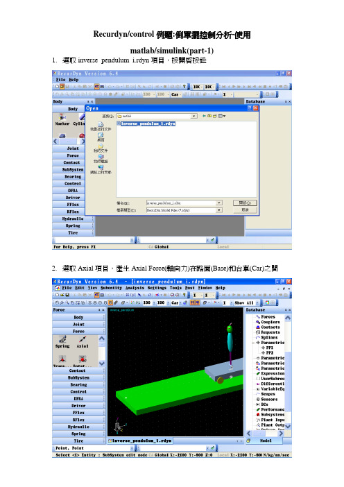
Recurdyn/control例題:倒單擺控制分析-使用matlab/simulink(part-1)1.選取inverse_pendulum_i.rdyn項目,按開啟按鈕2.選取Axial項目,產生Axial Force(軸向力)在路面(Base)和台車(Car)之間3.選取Body,Body,Point,Point項目,Body選地面、Body選車子、Point :2000,-100,0、Point : -500,-100,0(注意:軸向力方向(向右為正),因為建立軸向力時,方向是由左到右)4.選取Plant Input項目,按一下Add按鈕5.axial_force是系統的輸入廠(由控制迴路所決定),按一下確定按鈕6.選取Plant Output項目,按一下Add按鈕7.按兩下Add按鈕8.選取項目9. base.Marker1和bird.Marker1項目10.選取文字方塊,az(2,1):單擺的角度值,是系統的輸出廠(由RecurDyn計算),name:angle,按一下OK按鈕11.Plant Output List對話方塊開啟了,按一下確定按鈕12.選取axial1項目13.按一下EL按鈕14. 開啟Expression List對話方塊,按一下Create按鈕15. 開啟Expression對話方塊,按一下Add按鈕16. 軸向力內存函數是:pin(1);pin就是:Plant of Input,(1):就是axial_force。
選取文字方塊:pin(1)。
按一下OK按鈕17. 按一下確定按鈕18. 按一下確定按鈕19. 選取Cosim項目20. 選取Simulink項目,由Simulink啟動RecurDyn21. 輸出matlab*.m檔案,選取m-file to create plant block文字方塊,按delete鍵,輸入inverse_pendulum,按一下Export按鈕22. 按一下儲存(s)按鈕23. 按一下套用(A)按鈕,再按一下取消按鈕24. 記得存檔,關閉RecurDyn軟體------------------------------------------------------------------------------------------------------- Recurdyn/control例題:倒單擺控制分析-使用matlab/simulink(part-2)1.載入:inverse_pendulum.m2.鍵入:rdlib,rdlib是recurdyn plant控制,按enter鍵3.recurdyn_plant_7_視窗開啟4.鍵入:simulink,啟動simulink,按enter鍵5.simulink library browser視窗開啟,按一下simulink library browser按鈕6.按一下create a new model按鈕7.untitled視窗開啟8.拉進recurdyn plant,選取選項,建立pid迴路去控制軸向力大小,讓單擺可以動平衡9.選取Gain圖案進來,按ctrl+c鍵10.選取選項continuous\derivative、integrator圖案進來11.選取項目math operations\add圖案進來12.選取項目commonly used blocks\scope圖案進來,按ctrl+v鍵13.按add圖案快按兩下,function block parameters:add視窗開啟了,將++改成---,按一下OK按鈕14.連好線15.按Gain圖案快按兩下,function block parameters:gain視窗開啟,將1改成200,按一下OK按鈕16.按Gain1圖案快按兩下,function block parameters:gain視窗開啟,將1改成1,按一下OK按鈕17.按Gain2圖案快按兩下,function block parameters:gain視窗開啟,將1改成5,按一下OK按鈕18.按一下save(ctrl+s)按鈕19.輸入inverse_pendulum檔名,按Enter按鈕20.快按recurdyn plant block兩下,inverse_pendulum/recurdyn plant block視窗開啟,recurdyn plant圖案(紅色)是recurdyn與simulink之間的控制核心,快按兩下21. [ ]static analysis(事先進行靜力分析,之後再進行動力分析)[X ]recurdyn_show(計算過程可以啟動recurdyn畫面)[X ]recurdyn_animation(計算過程可以顯示動畫)之後按一下cancel按鈕,按一下關閉按鈕22.模擬時間5,按一下Start simulation按鈕23. RecurDyn 6.4視窗開啟,RecurDyn會自動載入模型,且可以看到計算過程中的動畫(很快就結束所以省略)24.快按scope圖案兩下,scope視窗開啟(scope是角度位移變化、scope1是軸向力輸出變化),Finish。
倒立摆系统的建模(拉格朗日方程)

系统的建模及性能分析倒立摆系统的构成及其参数1倒立摆系统的基本结构本设计所用到的倒立摆模型直线一级倒立摆系统。
整个系统是由6大部分所组成的一个闭环系统,包括计算机、数据采集卡、电源及功率放大器、直流伺服电机、倒立摆本体和两个光电编码器等模块。
如图2.1所示:图2.1 倒立摆系统的结构组成示意图Fig 2.1 Structure of the linear single inverted pendulum system2系统主要组成部分简介直线一级倒立摆装置如图2.2所示[13]:图2.2直线一级倒立摆装置Fig 2.2 Straight linear 1-stage inverted pendulum deviceQuanser倒立摆系统包含倒立摆本体、数据采集电控模块以及控制平台等三大部分,其中控制平台是由装有Quanser专用实时控制软件的通用PC机组成。
1.直线倒立摆主体倒立摆主体是由Quanser直线运动控制伺服单元IP02与直线一级摆杆组成,并配有专用的小车直线轨道。
这里主要介绍下Quanser直线运动控制伺服单元IP02(即倒立摆运动小车)及导轨的组成:图2.3伺服单元IP02的组成Fig 2.3 Servo unit IP02 parts编号名称英文(01)IP02小车IP02 Cart(02)不锈钢滑轨Stainless Steel Shaft(03)齿轮导轨Rack(04)小车位移齿轮Cart Position Pinion(05)小车电机传动齿轮Cart Motor Pinion(06)小车电机传动齿轮轴Cart Motor Pinion Shaft(07)摆杆传动轴Pendulum Axis(08)IP02小车位移编码器IP02 Cart Encoder(09)IP02摆杆角度编码器IP02 Pendulum Encoder(10)IP02小车位移编码器接口IP02 Cart Encoder Connector(11)IP02摆杆角度编码器接口IP02 Pendulum Encoder Connector(12)电机接口Motor Connector(13)直流伺服电机DC Motor(14)变速器Planetary Gearbox(15)直线滑轨支撑轴Linear Bearing图2.4系统导轨结构图Fig 2.4 System guide rail structure直线一级倒立摆系统的倒立摆的摆杆连接在IP02小车的摆杆连接套上,IP02小车由电机通过齿轮传动机构在导轨上来回运动,保持摆杆平衡。
基于MATLAB(矩阵实验室)的倒立摆控制系统仿真

基于MATLAB的倒立摆控制系统仿真摘要自动控制原理(包括经典部分和现代部分)是电气信息工程学院学生的一门必修专业基础课,课程中的一些概念相对比较抽象,如系统的稳定性、可控性、收敛速度和抗干扰能力等。
倒立摆系统是一个典型的非线性、强耦合、多变量和不稳定系统,作为控制系统的被控对象,它是一个理想的教学实验设备,许多抽象的控制概念都可以通过倒立摆直观地表现出来。
本文以一级倒立摆为被控对象,用经典控制理论设计控制器(PID控制器)的设计方法和用现代控制理论设计控制器(极点配置)的设计方法,通过MATLAB仿真软件的方法来实现。
关键词:一级倒立摆PID控制器极点配置Inverted pendulum controlling systemsimulation based on the MATLABABSTRACTAutomatic control theory (including classical parts and modern parts) is a compulsory specialized fundamental course of the students majored in electrical engineering. Some of the curriculum concept is relatively abstract, such as the stability, controllability, convergence rate and the anti-interference ability of system. Inverted pendulum system is a typical nonlinear, strong coupling, multivariable and unstable system. It is an ideal teaching experimental equipment as a controlled object, by which many abstract control concepts can be came out directly. This paper chose first-order inverted pendulum as the controlled object. First, the PID controller was designed with classical control theory. Then pole-assignment method was discussed with modern control theory. At last, the effectness of the two methods was verified by MATLAB simulation software.KEY WORDS: First-order inverted pendulum PID controller pole-assignment目录摘要 (I)ABSTRACT (II)1 绪论 (1)1.1倒立摆的控制方法 (1)1.2 MATLAB/Simulink简介 (2)1.3 主要内容 (3)2一级倒立摆 (3)2.1 实验设备简介 (3)3直线一级倒立摆的数学模型 (4)3.1直线一级倒立摆数学模型的推导 (4)3.1.1 微分方程模型 (6)3.1.2 传递函数模型 (7)3.1.3 状态空间数学模型 (8)3.2系统阶跃响应分析 (10)4 直线一级倒立摆PID控制器设计 (14)4.1 PID控制分析 (14)4.2PID控制参数设定及MATLAB仿真 (17)5直线一级倒立摆状态空间极点配置控制器设计 (20)5.1 状态空间分析 (21)5.2极点配置及MATLAB仿真 (22)6总结 (26)致谢 (27)参考文献 (28)1 绪论倒立摆起源于20世纪50年代,是一个典型的非线性、高阶次、多变量、强耦合、不稳定的动态系统,能有效地反映诸如稳定性、鲁棒性等许多控制中的关键问题,是检验各种控制理论的理想模型。
一级倒立摆课程设计--倒立摆PID控制及其Matlab仿真
一级倒立摆课程设计--倒立摆PID控制及其Matlab仿真倒立摆PID控制及其Matlab仿真学生姓名:学院:电气信息工程学院专业班级:专业课程:控制系统的MATLAB仿真与设计任课教师:2014 年 6 月 5 日倒立摆PID控制及其Matlab仿真Inverted Pendulum PID Control and ItsMatlab Simulation摘要倒立摆系统是一个典型的快速、多变量、非线性、不稳定系统,对倒立摆的控制研究无论在理论上和方法上都有深远的意义。
本论文以实验室原有的直线一级倒立摆实验装置为平台,重点研究其PID 控制方法,设计出相应的PID控制器,并将控制过程在MATLAB上加以仿真。
本文主要研究内容是:首先概述自动控制的发展和倒立摆系统研究的现状;介绍倒立摆系统硬件组成,对单级倒立摆模型进行建模,并分析其稳定性;研究倒立摆系统的几种控制策略,分别设计了相应的控制器,以MATLAB为基础,做了大量的仿真研究,比较了各种控制方法的效果;借助固高科技MATLAB实时控制软件实验平台;利用设计的控制方法对单级倒立摆系统进行实时控制,通过在线调整参数和突加干扰等,研究其实时性和抗千扰等性能;对本论文进行总结,对下一步研究作一些展望。
关键词:倒立摆;PID控制器;MATLAB仿真设计报告正文1.简述一级倒立摆系统的工作原理;倒立摆是一个数字式的闭环控制系统,其工作原理为:角度、位移信号检测电路获取后,由微分电路获取相应的微分信号。
这些信号经A/D转换器送入计算机,经过计算及内部的控制算法解算后得到相应的控制信号,该信号经过D/A变换、再经功率放大由执行电机带动皮带卷拖动小车在轨道上做往复运动,从而实现小车位移和倒立摆角位移的控制。
2.依据相关物理定理,列写倒立摆系统的运动方程;2lO1小车质量为M ,倒立摆的质量为m ,摆长为2l ,小车的位置为x ,摆的角度为θ,作用在小车水平方向上的力为F ,1O 为摆杆的质心。
滑模控制 二阶倒立摆 matlab
滑模控制二阶倒立摆 matlab滑模控制是一种常用的控制方法,在控制二阶倒立摆中也可以得到很好的应用。
通过加入滑模控制器可以提高控制系统的稳定性和鲁棒性。
在 Matlab 中,可以使用 Simulink 来进行二阶倒立摆的仿真和控制器设计。
具体步骤如下:1. 搭建二阶倒立摆的模型,包括小车、摆杆和配重块等组成部分。
2. 设计 PID 控制器,作为基准控制器用于比较滑模控制器的性能;3. 按照滑模控制器设计的思路,搭建滑模控制器模型,其中包括滑模面、滑模控制律等组成部分。
4. 将滑模控制器与二阶倒立摆模型进行连接,并进行仿真。
实现过程中的代码如下:1. 建立模型:使用 Simulink 中的组件、信号源、仿真器等构建二阶倒立摆控制系统模型。
2. PID 控制器设计:```matlabKp = 1.5;Ki = 0.01;Kd = 0.2;pid_controller = pid(Kp, Ki, Kd);```3. 滑模控制器设计:```matlabs = 0.1;r = 0.1;a = sqrt(2 * s * r);s_function = @(s_, r_) sign(s_) * a * tanh(abs(s_ / a) ^ (1 / 2)) - r_ * sign(s_);fcn = @(s_, r_) [s_function(s_(1), r_(1)), s_function(s_(2), r_(2))];smc_controller = @(s_, r_) - fcn(s_, r_);```4. 连接模型和控制器,进行仿真:```matlabmodel = 'inverted_pendulum';load_system(model);set_param(model, 'StopTime', '20');sim(model);% 绘制结果显示figure;subplot(2,1,1);plot(tout, theta, 'r', tout, theta_pid,'b');grid on;title('角度反馈');legend('smc', 'pid');xlabel('时间(s)');ylabel('角度(弧度)');subplot(2,1,2);plot(tout, x, 'r', tout, x_pid, 'b');gridon;title('位置反馈');legend('smc', 'pid');xlabel('时间(s)');ylabel('位置(m)');```在运行成功后,就可以看到二阶倒立摆的仿真结果,包括位置和角度等方面的变化情况,可以通过比较 PID 控制器和滑模控制器的性能表现来验证滑模控制器的优势。
毕业设计基于模糊控制的倒立摆系统及MATLAB仿真

摘要倒立摆系统是研究控制理论的一种典型的实验装置,广泛应用于控制理论研究,航空航天控制等领域,其控制研究对于自动化控制领域具有重要的价值。
然而,倒立摆装置是一个绝对不稳定系统,具有高阶次、非线性、强耦合等特性,本文应用模糊控制策略对其进行控制研究。
本文应用牛顿力学定律建立了直线一级倒立摆的状态方程数学模型并推导了简化的传递函数数学模型,分析了其稳定性,可控性和可观测性。
研究了控制系统整体结构,建立了模糊控制器,在MATLAB平台上对模糊控制系统进行了仿真研究,并对获得的控制系统输出图进行了性能分析。
关键词:一阶倒立摆,数学模型,模糊控制, MATLAB仿真AbstractInverted pendulum control system is to study the theory of a typical experimental device, widely used in control theory, the field of aerospace control, its control is important for the automation and control value. However, the inverted pendulum device is an absolute unstable system, with high time, nonlinear, strong coupling and other features, this fuzzy control strategy to control research.In this paper, Newton's laws of mechanics to establish a line-level inverted pendulum equation of state mathematical model to derive the simplified transfer function model to analyze its stability, controllability and observability. Of the control system as a whole structure of a fuzzy controller, in the MATLAB platform for fuzzy control system was simulated, and access control system output graph of the performance analysis.Keywords: inverted pendulum, mathematical model, fuzzy control, MATLAB simulation目录摘要 (i)Abstract (ii)第一章倒立摆系统简介 (1)1.1倒立摆系统概述 (1)1.2倒立摆的控制目标及研究意义 (1)1.3倒立摆系统控制方法简介 (2)1.4论文的主要工作 (4)第二章模糊控制概述 (6)2.1控制理论简介 (6)2.1.1经典控制理论 (6)2.1.2现代控制理论 (6)2.1.3模糊控制与经典控制理论的比较 (8)2.2模糊控制的数学基础 (9)2.2.1模糊子集与运算 (9)2.2.2模糊关系与模糊关系合成 (11)2.2.3模糊推理 (12)第三章控制系统分析与模糊控制方法研究 (15)3.1控制系统结构及工作原理 (15)3.1.1控制系统结构 (15)3.1.2模糊控制器的工作原理 (16)3.2精确量的模糊化 (17)3.2.1模糊控制器的语言变量 (17)3.2.2量化因子与比例因子 (17)3.2.3语言变量值的选取 (18)3.2.4语言变量论域上的模糊子集 (18)3.3常见的模糊控制规则 (19)3.4输出信息的模糊判决 (20)3.4.1基于推理合成规则进行模糊推理 (20)3.4.2输出信息的模糊判决 (20)3.5本章小结 (21)第四章倒立摆系统建模 (21)4.1常见的倒立摆类型 (21)4.2倒立摆系统建模 (23)4.3系统可控性分析 (27)第五章倒立摆模糊控制器的设计及仿真 (29)5.1倒立摆的稳定模糊控制器的设计 (29)5.1.1位置模糊控制器的设计 (29)5 .1.2角度模糊控制器的设计 (34)5.1.3稳定控制器的实现 (34)5. 2一级倒立摆系统仿真 (35)5.2.1 Simulink简介 (36)5.2.2系统仿真 (37)第六章总结 (44)致谢 (45)参考文献 ......................................................................................................................... 错误!未定义书签。
MATLAB的虚拟倒立摆仿真

VR ML 是虚拟现实建模语言,用来建立虚构 的三维场景的模型。VR ML 文件是虚拟空间的文 本性描述,它可由任何一个文本编辑器(如记事本 等) 生 成,文 件 以“. Wrl ”为 扩 展 名。 但 通 过
Machine buil ding Auto mation ,Dec 2004 ,33(6 ):101 !102 ,105
可选择的虚拟世界对话框打开,选择文件“vrpend . wrl ”并且点击 0 pen 。在模块参数“Vr :Si nk ”对话 框内,点击 Appl y 。这时一个 Vr ML 目录树出现 在右边,如图3 所示。目录树中包含有相关的虚拟 现实场景的结构。在 Pendul u m 的左边按“+ ”标 记,那么倒立摆树目录展开。现在我们可以看到倒
·电气技术与自动化·
张宏立·MATLAB 的虚拟倒立摆仿真
MATLAB 的虚拟倒立摆仿真
张宏立
(新疆大学电气工程学院,新疆 乌鲁木齐 830008 )
摘 要:利用 MATLAB 提供的 V- Real m Buil der 建立倒立摆三维虚拟场景,用 MATLAB 的虚 拟现实工具箱将倒立摆三维虚拟场景和Si muli nk 中倒立摆仿真模型连接起来,实现了虚拟倒 立摆的仿真。
·101 ·
·电气技术与自动化·
张宏立·MATLAB 的虚ห้องสมุดไป่ตู้倒立摆仿真
Vr ML 建模是非常麻烦的事情,不仅要编写大量 代码,而且不能所见即所得。MATLAB 中自带一 个强大的三维物体构造软件包 V- real m Buil der , 它提供了一个集成开发环境,无论是专家还是初学
者都很容易学会使用,它生成的三维物体和虚拟世
Si muli nk 是一个用来对动态系统进行建模、仿 真和分析的软件包,它为用户提供了用方框图进行 建模的图形接口,采用这种结构画模型就像用笔和 纸来画一样容易,与传统的仿真软件包用微分方程 和差分方程建模相比,具有更直观、方便和灵活的 优点。模拟一个Si muli nk 模型产生动态系统的信 号数据,将Si muli nk 模型连接到一个虚拟场景,就 可以使用此数据控制和操纵此虚拟场景。图2 是 完整的Si muli nk 模型,它里面最重要的模块是 Vr Si nk 模块,这是虚拟现实工具箱中的信号转换模 块,它的功能是将 Si muli nk 中的信号送到虚拟场 景中。当产生一个虚拟场景和一个 Si muli nk 模型 后,那么就 可 以 通 过 虚 拟 现 实 工 具 箱 将 其 连 接 起
Inverted pendulum倒立摆的matlab建模
ECE451 Controll EngineeringInverted pendulum09/29/2013Introduction:Inverted pendulum is a typical fast, multi-varaibles, nonlinear, unstable system, it has significant meaning. We choose the PID controller to fot the inverted pendulum.Assume the input is a step signal , the gravitational acceleration g=9.8m/s^2 and linearize the nonlinear model around the operating point.1.Mathematic ModlingM mass of the car0.5 kgm mass of the pendulum0.2 kgb coefficient of friction for cart0.1 N/m/secl length to pendulum center of mass0.3 mI mass moment of inertia of the pendulum 0.006 kg.m^2F force applied to the cartx coordinate of cart positionθpendulum angle from vertical (down)N and F are the force from horizontal and vertical direction.(x+l sinθ)N=m d2dt2Force analysisConsider the horizontal direction cart force, we get the equation:Mẍ=F−bẋ−NConsider the horizontal direction pendulum force, we get the equation:N=mẍ+mlθcosθ−mlθ2sinθTo get rid of P and N, we get this equation:−Pl sinθ−Nl cosθ=IθMerge these two equations, about to P And N, to obtain a second motion equation:(l+ml2)θ+mgl sinθ=−mlẍcosθu to represent the controlled object with the input force F, linearized two motion equationsApply Laplace transform to the equation aboveThe transfer function of angle and positionLet v = ẍput the equation above into the second equationWe get the transfer functionState space equation:Solve the algebraic equation, obtain solution as follows:Finally we get the system state space equations.2. PID Controller DesignWe now design a PID controller for the inverted pendulum system.KD(s) is the transfer function of the controller.G(s) is the transfer function of the controlled car.Considering that the input r(s) =0, the block diagram can be transformed as: The output of the system is()()()()()()()()()()()()()()()()s F num num PID den denPID denPIDnum s F den denPID num num PID den s F s G s kD s G s y +=+=+=11num —the numerator of the object den —the denominator of the objectnumPID – the numerator of the PID controller transfer function denPID – the denominator of the PID controller transfer function The object transfer function is()()()()den num sq bmgl s q mgl M m s q ml I b s sqml s U s =-+-++=Φ23242,in which [()()()]22ml ml I M m q -++=.PID Controller Transfer Function is()22s K s K s K s K K s K s KD Ip D I P D ++=++=Now, we add the car’s position as another output, we getin which G1 is the transfer function of the pendulum, G2 is the transfer function of the car.The output of the car’s position is()()()()()()()()()()s F den denPID num numPID den s F s G s KD s G s X 11221211+=+=in which, num1,den1,num2,den2 are separately mean the controlled object 1 andobject 2 and PID controller‘s numerators and denominators.From ()()()s s g ml ml I s X Φ⎥⎦⎤⎢⎣⎡-+=22, we could get thatIn which,[()()()]22ml ml I M m q -++=.We can easily simplified the equation as()()()()()()()()s F num numPID k den denPID denPID num s X 12+=3. Matlab SimulationIn design, the cart's position will be ignored. Under these conditions, the designcriteria are:1) settling time is less than 5 seconds2) pendulum should not move more than 0.05 radians away from the vertical When kd=1,k=1,ki=1:numc1=4.5455 0 0 0, denc1=1 4.7273 -26.6364 0.0909 0 0, num2= -1.8182 0 44.5455 0, denc2=1 4.7273 -26.6364 0.0909 0()()()()()()sqbmgl s q mgl M m s q ml I b s sq bmgl s q ml I s U s X s G -+-++-+==2324222Then we tried many times to adjust the parameter to satisfy the requirements: Ts <=5 s and overshoot M<0.05.We find the optimal parameters of kd,k,ki which is the second situation.2. When kd=20,k=300,ki=1:Numc1= 4.5455 0 0 0, denc1=0.001 0.09111.3325 0.0001 0 0, numc2= -1.8182 0 44.5455 0, denc2=0.001 0.09111.3325 0.0001 0 0The results:Matlab codesM=0.5;m=0.2;b=0.1;I=0.006;g=9.8;l=0.3;q=(M+m)*(I+m*l^2)/q-(m*l)^2;num1=[m*l/q 0 0];den1=[1 b*(I+m*l^2)/q-(M+m)*m*g*l/q-b*m*g*l/q 0]; num2=[-(I+m*l^2)/q 0 m*g*l/q];den2=den1;kd=1;k=1;ki=1;numPID=[kd k ki];denPID=[1 0];numci=conv (num1 denPID);denc1=polyadd(conv(denPID,den1),conv(numPID,num1)); t=0:0.1:20;figure(1)impulse(numc1,denc1,t)title(‘Angle’)figure(2)impulse(numc2,denc2,t)title(‘Position’)M=0.5;m=0.2;b=0.1;I=0.006;g=9.8;l=0.3;q=(M+m)*(I+m*l^2)/q-(m*l)^2;num1=[m*l/q 0 0];den1=[1 b*(I+m*l^2)/q-(M+m)*m*g*l/q-b*m*g*l/q 0]; num2=[-(I+m*l^2)/q 0 m*g*l/q];den2=den1;kd=20;k=300;ki=1;numPID=[kd k ki];denPID=[1 0];numci=conv (num1 denPID);denc1=polyadd(conv(denPID,den1),conv(numPID,num1));t=0:0.1:20;figure(1)impulse(numc1,denc1,t)title(‘Angle’)figure(2)impulse(numc2,denc2,t)title(‘Position’)Simulation:We will build a closed-loop model with reference input of pendulum position and a disturbance force applied to the cart.We now begin to simulate the closed-loop system. The physical parameters are set as follows.M=0.5, m=0.2, b=0.1, I=0.006, g=9.8, l=0.3After 20s simulation, we see the response as followThe response is very much like what have been done in Matlab codes.。
- 1、下载文档前请自行甄别文档内容的完整性,平台不提供额外的编辑、内容补充、找答案等附加服务。
- 2、"仅部分预览"的文档,不可在线预览部分如存在完整性等问题,可反馈申请退款(可完整预览的文档不适用该条件!)。
- 3、如文档侵犯您的权益,请联系客服反馈,我们会尽快为您处理(人工客服工作时间:9:00-18:30)。
ECE451 Controll EngineeringInverted pendulum09/29/2013Introduction:Inverted pendulum is a typical fast, multi-varaibles, nonlinear, unstable system, ithas significant meaning. We choose the PID controller to fot the inverted pendulum. Assume the input is a step signal , the gravitational acceleration g=9.8m/s^2 and linearize the nonlinear model around the operating point.1.Mathematic ModlingM mass of the car 0.5 kgm mass of the pendulum 0.2 kgb coefficient of friction for cart 0.1 N/m/secl length to pendulum center of mass 0.3 mI mass moment of inertia of the pendulum 0.006 kg.m^2F force applied to the cartx coordinate of cart positionθpendulum angle from vertical (down)N and F are the force from horizontal and vertical direction.)Force analysisConsider the horizontal direction cart force, we get the equation:Consider the horizontal direction pendulum force, we get the equation:To get rid of P and N, we get this equation:Merge these two equations, about to P And N, to obtain a second motion equation:u to represent the controlled object with the input force F, linearized two motion equationsApply Laplace transform to the equation aboveThe transfer function of angle and positionLet v =put the equation above into the second equationWe get the transfer functionState space equation:Solve the algebraic equation, obtain solution as follows:Finally we get the system state space equations.2. PID Controller DesignWe now design a PID controller for the inverted pendulum system.KD(s) is the transfer function of the controller.G(s) is the transfer function of the controlled car.Considering that the input r(s) =0, the block diagram can be transformed as: The output of the system is()()()()()()()()()()()()()()()()sFnumnumPIDdendenPIDdenPIDnumsFdendenPIDnumnumPIDdennumsFsGskDsGsy+=+=+=11num —the numerator of the objectden —the denominator of the objectnumPID – the numerator of the PID controller transfer functiondenPID – the denominator of the PID controller transfer functionThe object transfer function is()()()()dennumsqbmglsqmglMmsqmlIbssqmlsUs=-+-++=Φ23242,in which[()()()]22mlmlIMmq-++=.PID Controller Transfer Function is()22sKsKsKsKKsKsKD IpDIPD++=++=Now, we add the car’s position as another output, we getin which G1 is the transfer function of the pendulum, G2 is the transfer function of the car.The output of the car’s position is()()()()()()()()()()sFdendenPIDnumnumPIDdennumsFsGsKDsGsX11221211+=+=in which, num1,den1,num2,den2 are separately mean the controlled object 1 and object 2 and PID controller‘s numerators and denominators.From ()()()s s g ml ml I s X Φ⎥⎦⎤⎢⎣⎡-+=22, we could get thatIn which,[()()()]22ml ml I M m q -++=.We can easily simplified the equation as()()()()()()()()s F num numPID k den denPID denPID num s X 12+=3. Matlab SimulationIn design, the cart's position will be ignored. Under these conditions, the design criteria are:1) settling time is less than 5 seconds2) pendulum should not move more than 0.05 radians away from the vertical When kd=1,k=1,ki=1:numc1=4.5455 0 0 0, denc1=1 4.7273 -26.6364 0.0909 0 0, num2= -1.8182 0 44.5455 0, denc2=1 4.7273 -26.6364 0.0909 0()()()()()()s qbmgl s q mgl M m s q ml I b s s qbmgls q ml I s U s X s G -+-++-+==2324222Then we tried many times to adjust the parameter to satisfy the requirements: Ts <=5 s and overshoot M<0.05.We find the optimal parameters of kd,k,ki which is the second situation.2. When kd=20,k=300,ki=1:Numc1= 4.5455 0 0 0, denc1=0.001 0.09111.3325 0.0001 0 0, numc2= -1.8182 0 44.5455 0, denc2=0.001 0.09111.3325 0.0001 0 0The results:Matlab codesM=0.5;m=0.2;b=0.1;I=0.006;g=9.8;l=0.3;q=(M+m)*(I+m*l^2)/q-(m*l)^2;num1=[m*l/q 0 0];den1=[1 b*(I+m*l^2)/q-(M+m)*m*g*l/q-b*m*g*l/q 0];num2=[-(I+m*l^2)/q 0 m*g*l/q];den2=den1;kd=1;k=1;ki=1;numPID=[kd k ki];denPID=[1 0];numci=conv (num1 denPID);denc1=polyadd(conv(denPID,den1),conv(numPID,num1)); t=0:0.1:20;figure(1)impulse(numc1,denc1,t)title(‘Angle’)figure(2)impulse(numc2,denc2,t)title(‘Position’)M=0.5;m=0.2;b=0.1;I=0.006;g=9.8;l=0.3;q=(M+m)*(I+m*l^2)/q-(m*l)^2;num1=[m*l/q 0 0];den1=[1 b*(I+m*l^2)/q-(M+m)*m*g*l/q-b*m*g*l/q 0]; num2=[-(I+m*l^2)/q 0 m*g*l/q];den2=den1;kd=20;k=300;ki=1;numPID=[kd k ki];denPID=[1 0];numci=conv (num1 denPID);denc1=polyadd(conv(denPID,den1),conv(numPID,num1)); t=0:0.1:20;figure(1)impulse(numc1,denc1,t)title(‘Angle’)figure(2)impulse(numc2,denc2,t)title(‘Position’)Simulation:We will build a closed-loop model with reference input of pendulum position and a disturbance force applied to the cart.We now begin to simulate the closed-loop system. The physical parameters are set as follows.M=0.5, m=0.2, b=0.1, I=0.006, g=9.8, l=0.3After 20s simulation, we see the response as followThe response is very much like what have been done in Matlab codes.。