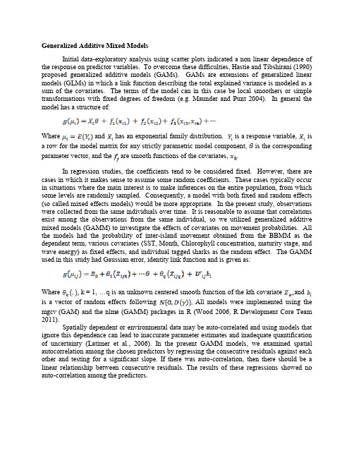
Generalized Additive Models

of the tted curve. The right panel of gure 1 shows a cubic spline t to the data.
What value of did we use in gure 1? In fact it is not convenient to express the desired smoothness of f in terms of , as the meaning of
* *
*
*
*
*
*** *
* *
*
0.5
1.5
2.5
x
y
-1
0
1
*
* **
*
** * ** * **
** * **
*
*****
* * **
** **
*
** * ** **********
*
* ****
*
******
* *
*
*
*
*
*** *
* *
*
0.5
1.5
2.5
x
-1
Figure 1: Left panel shows a ctitious scatterplot of an outcome measure y plotted against a prognostic factor x. In the right panel, a scatterplot smooth has been added to describe the trend of y on x.
fቤተ መጻሕፍቲ ባይዱctor. of y on
We wish x. If we
to were
ta to
smooth nd the
curve curve
f (x) that
that summarizes simply minimizes
tPhe(ydie?pefn(dxein))c2e,
the result would be an interpolating curve that would not be smooth at all.
Department of Statistics and Division of Biostatistics, Stanford University, Stanford California 94305; trevor@
yDepartment of Preventive Medicine and Biostatistics, and Department of Statistics, University of Toronto; tibs@; tibs@
depends on the units of the prognostic factor x. Instead, it is possible to de ne an \e ective number of parameters" or \degrees of freedom" of a cubic spline smoother, and then use a numerical search to determine the value of to yield this number. In gure 1 we chose the e ective number of parameters to be 5. Roughly speaking, this means that the complexity of the curve is about the same as a polynomial regression of degrees 4. However, the cubic spline smoother \spreads out" its parameters in a more even manner, and hence is much more exible than a polynomial regression. Note that the degrees of freedom of a smoother need not be an integer.
Generalized additive models
Trevor Hastie
and
Robert Tibshirani y
1 Introduction
In the statistical analysis of clinical trials and observational studies, the identi cation and adjustment for prognostic factors is an important component. Valid comparisons of di erent treatments requires the appropriate adjustment for relevant prognostic factors. The failure to consider important prognostic variables, particularly in observational studies, can lead to errors in estimating treatment di erences. In addition, incorrect modeling of prognostic factors can result in the failure to identify nonlinear trends or threshold e ects on survival.
dataset. Fast and stable numerical procedures are available for computation
2
1
0
y
*
* **
*
*** ** * **
** * **
*
*****
* * **
** **
*
** * ** **********
*
* ****
*
******
IbtygPov(eyrin?s
the tradeo f(xi))2) and
between the goodness of t wiggliness of the function.
to the Larger
data (as values of
measured force f
to be smoother.
The above discussion tells how to t a curve to a single prognostic factor. With multiple prognostic factors, if xij denotes the value of the jth prognostic
This article describes exible statistical methods that may be used to identify and characterize the e ect of potential prognostic factors on an outcome variable. These methods are called \generalized additive models", and extend the traditional linear statistical model. They can be applied in any setting where a linear or generalized linear model is typically used. These settings include standard continuous response regression, categorical or ordered categorical response data, count data, survival data and time series.
We rst give some background on the methodology, and then discuss the
details of the logistic regression model and its generalization. Some related
developments are discussed in the last section.
1
opatdrheddeirticitvteoecrhmonofidqtuehleerse)fopmrlamocdePeslPtxhjxejje,
ects of prognostic factors xj in terms of a linear
where j with
Pthfej
j
(xj
are parameters. The generalized ) where fj is a unspeci ed (\non-
setting, and then indicate how it is used in generalized additive modeling.
Suppose that we have a scatterplot of points (xi; yi) like that shown in gure 1. Here y is a response or outcome variable, and x is a prognostic
For any value of , the solution to (1) is a cubic spline, i.e., a piecewise