信号与系统(奥本海默第二版)第7章
奥本海姆目录
《信号与系统》第1章信号与系统1.0 引言1.1 连续时间和离散时间信号1.1.1 举例与数学表示1.1.2 信号能量与功率1.2 自变数的变换1.2.1 自变数变换举例1.2.2 周期信号1.2.3 偶信号与奇信号1.3 指数信号与正弦信号1.3.1 连续时间复指数信号与正弦信号1.3.2 离散时间复指数信号与正弦信号1.3.3 离散时间复指数序列的周期性质1.4 单位冲激与单位阶跃函数1.4.1 离散时间单位脉冲和单位阶跃序列1.4.2 连续时间单位阶跃和单位冲激函数1.5 连续时间和离散时间系统1.5.1 简单系统举例1.5.2 系统的互联1.6 基本系统性质1.6.1 记忆系统与无记忆系统1.6.2 可逆性与可逆系统1.6.3 因果性1.6.4 稳定性1.6.5 时不变性1.6.6 线性1.7 小结习题第2章线性时不变系统2.0 引言2.1 离散时间LTI系统:卷积和2.1.1 用脉冲表示离散时间信号2.1.2 离散时间LTI系统的单位脉冲响应及卷积和表示2.2 连续时间LTI系统:卷积积分2.2.1 用冲激表示连续时间信号2.2.2 连续时间LTI系统的单位冲激响应及卷积积分表示2.3 线性时不变系统的性质2.3.1 交换律性质2.3.2 分配律性质2.3.3 结合律性质2.3.4 有记忆和无记忆LTI系统2.3.5 LTL系统的可逆性2.3.6 LTI系统的因果性2.3.7 LTI系统的稳定性2.3.8 LTI系统的单位阶跃响应2.4 用微分和差分方程描述的因果LTI系统2.4.1 线性常系数微分方程2.4.2 线性常系数差分方程2.4.3 用微分和差分方程描述的一阶系统的方框图表示2.5 奇异函数2.5.1 作为理想化短脉冲的单位冲激2.5.2 通过卷积定义单位冲激2.5.3 单位冲激偶和其它的奇异函数2.6 小结习题第3章周期信号的傅里叶级数表示3.0 引言3.1 历史回顾3.2 LTI系统对复指数信号的响应3.3 连续时间周期信号的傅里叶级数表示3.3.1 成谐波关系的复指数信号的线性组合3.3.2 连续时间周期信号傅里叶级数表示的确定3.4 傅里叶级数的收敛3.5 连续时间傅里叶级数性质3.5.1 线性3.5.2 时移性质3.5.3 时间反转3.5.4 时域尺度变换3.5.5 相乘3.5.6 共轭及共轭对称性3.5.7 连续时间周期信号的帕斯瓦尔定理3.5.8 连续时间傅里叶级数性质列表3.5.9 举例3.6 离散时间周期信号的傅里叶级数表示3.6.1 成谐波关系的复指数信号的线性组合3.6.2 周期信号傅里叶级数表示的确定3.7 离散时间傅里叶级数性质3.7.1 相乘3.7.2 一阶差分3.7.3 离散时间周期信号的帕斯瓦尔定理3.7.4 举例3.8 傅里叶级数与LTI系统3.9 滤波3.9.1 频率成形滤波器3.9.2 频率选择性滤波器3.10 用微分方程描述的连续时间滤波器举例3.10.1 简单RC低通滤波器3.10.2 简单RC高通滤波器3.11 用差分方程描述的离散时间滤波器举例3.11.1 一阶递归离散时间滤波器3.11.2 非递归离散时间滤波器3.12 小结习题第4章连续时间傅里叶变换4.0 引言4.1 非周期信号的表示:连续时间傅里叶变换4.1.1 非周期信号傅里叶变换表示的导出4.1.2 傅里叶变换的收敛4.1.3 连续时间傅里叶变换举例4.2 周期信号的傅里叶变换4.3 连续时间傅里叶变换性质4.3.1 线性4.3.2 时移性质4.3.3 共轭及共轭对称性4.3.4 微分与积分4.3.5 时间与频率的尺度变换4.3.6 对偶性4.3.7 帕斯瓦尔定理4.4 卷积性质4.4.1 举例4.5 相乘性质4.5.1 具有可变中心频率的频率选择性滤波4.6 傅里叶变换性质和基本傅里叶变换对列表4.7 由线性常系数微分方程表征的系统4.8 小结习题第5章离散时间傅里叶变换5.0 引言5.1 非周期信号的表示:离散时间傅里叶变换5.1.1 离散时间傅里叶变换的导出5.1.2 离散时间傅里叶变换举例5.1.3 关于离散时间傅里叶变换的收敛问题5.2 周期信号的傅里叶变换5.3 离散时间傅里叶变换性质5.3.1 离散时间傅里叶变换的周期性5.3.2 线性5.3.3 时移与频移性质5.3.4 共轭与共轭对称性5.3.5 差分与累加5.3.6 时间反转5.3.7 时域扩展5.3.8 频域微分5.3.9 帕斯瓦尔定理5.4 卷积性质5.4.1 举例5.5 相乘性质5.6 傅里叶变换性质和基本傅里叶变换对列表5.7 对偶性5.7.1 离散时间傅里叶级数的对偶性5.7.2 离散时间傅里叶变换和连续时间傅里叶级数之间的对偶性5.8 由线性常系数差分方程表征的系统5.9 小结习题第6章信号与系统的时域和频域特性6.0 引言6.1 傅里叶变换的模和相位表示6.2 LTI系统频率响应的模和相位表示6.2.1 线性与非线性相位6.2.2 群时延6.2.3 对数模和波特图6.3 理想频率选择性滤波器的时域特性6.4 非理想滤波器的时域和频域特性讨论6.5 一阶与二阶连续时间系统6.5.1 一阶连续时间系统6.5.2 二阶连续时间系统6.5.3 有理型频率响应的波特图6.6 一阶与二阶离散时间系统6.6.1 一阶离散时间系统6.6.2 二阶离散时间系统6.7 系统的时域分析与频域分析举例6.7.1 汽车减震系统的分析6.7.2 离散时间非递归滤波器举例6.8 小结习题第7章采样7.0 引言7.1 用信号样本表示连续时间信号:采样定理7.1.1 冲激串采样7.1.2 零阶保持采样7.2 利用内插由样本重建信号7.3 欠采样的效果:混迭现象7.4 连续时间信号的离散时间处理7.4.1 数字微分器7.4.2 半采样间隔延时7.5 离散时间信号采样7.5.1 脉冲串采样7.5.2 离散时间抽取与内插7.6 小结习题第8章通信系统8.0 引言8.1 复指数与正弦幅度调制8.1.1 复指数载波的幅度调制8.1.2 正弦载波的幅度调制8.2 正弦AM的解调8.2.1 同步解调8.2.2 异步解调8.3 频分多路复用8.4 单边带正弦幅度调制8.5 用脉冲串作载波的幅度调制8.5.1 脉冲串载波调制8.5.2 时分多路复用8.6 脉冲幅度调制8.6.1 脉冲幅度已调信号8.6.2 在PAM系统中的码间干扰8.6.3 数字脉冲幅度和脉冲编码调制8.7 正弦频率调制8.7.1 窄带频率调制8.7.2 宽带频率调制8.7.3 周期方波调制信号8.8 离散时间调制8.8.1 离散时间正弦幅度调制8.8.2 离散时间调制转换8.9 小结习题第9章拉普拉斯变换9.0 引言9.1 拉普拉斯变换9.3 拉普拉斯反变换9.4 由零极点图对傅里叶变换进行几何求值9.4.1 一阶系统9.4.2 二阶系统9.4.3 全通系统9.5 拉普拉斯变换的性质9.5.1 线性9.5.2 时移性质9.5.3 S域平移9.5.4 时域尺度变换9.5.5 共轭9.5.6 卷积性质9.5.7 时域微分9.5.8 S域微分9.5.9 时域积分9.5.10 初值与终值定理9.5.11 性质列表9.6 常用拉普拉斯变换对9.7 用拉普拉斯变换分析和表征LTI系统9.7.1 因果性9.7.2 稳定性9.7.3 由线性常系数微分方程表征的LTI系统9.7.4 系统特性与系统函数的关系举例9.7.5 巴特沃兹滤波器9.8 系统函数的代数属性与方框图表示9.8.1 LTI系统互联的系统函数9.8.2 由微分方程和有理系统函数描述的因果LTI系统的方框图表示9.9单边拉普拉斯变换9.9.1 单边拉普拉斯变换举例9.9.3 利用单边拉普拉斯变换求解微分方程9.10 小结习题第10章Z变换10.0 引言10.1 Z变换10.2 Z变换的收敛域10.3 Z反变换10.4 由零极点图对傅里叶变换进行几何求值10.4.1 一阶系统10.4.2 二阶系统10.5 Z变换的性质10.5.1 线性10.5.2 时移性质10.5.3 Z域尺度变换10.5.4 时间反转10.5.5 时间扩展10.5.6 共轭10.5.7 卷积性质10.5.8 Z域微分10.5.9 初值定理10.5.10 性质小结10.6 几个常用Z变换对10.7 利用Z变换分析与表征LTI系统10.7.1 因果性10.7.2 稳定性10.7.3 由线性常系数差分方程表征的LTI系统10.7.4 系统特性与系统函数的关系举例10.8 系统函数的代数属性与方框图表示10.8.1 LTI系统互联的系统函数10.8.2 由差分方程和有理系统函数描述的因果LTI系统的方框图表示10.9 单边Z变换10.9.1 单边Z变换和单边Z反变换举例10.9.2 单边Z变换性质10.9.3 利用单边Z变换求解差分方程10.10 小结习题第11章线性反馈系统11.0 引言11.1 线性反馈系统11.2 反馈的某些应用及结果11.2.1 逆系统设计11.2.2 非理想组件的补偿11.2.3 不稳定系统的稳定11.2.4 采样数据反馈系统11.2.5 跟踪系统11.2.6 反馈引起的不稳定11.3 线性反馈系统的根轨迹分析法11.3.1 一个例子11.3.2 死循环极点方程11.3.3 根轨迹的端点:K=0和|K|=+∞时的死循环极点11.3.4 角判据11.3.5 根轨迹的性质11.4 奈奎斯特稳定性判据11.4.1 围线性质11.4.2 连续时间LTI反馈系统的奈奎斯特判据11.4.3 离散时间LTI反馈系统的奈奎斯特判据11.5 增益和相位裕度11.6 小结。
信号与系统奥本海姆英文版课后答案chapter7
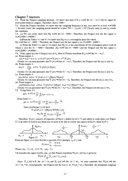
137Chapter 7 Answers7.1 From the Nyquist sampling theorem , we know that only if X (j w)=0 for |w| > w s /2 will be signal be recoverable from its samples. Therefore, X(jw)>5000л.7.2 From the Nyquist theorem ,we know that the sampling frequency in this case must be at least w s =2000п.In other words ,the sampling period should be at most T=2п/ (w s )=1*10-3.Clearly ,only (a) and (e) satisfy this condition.7.3 (a) We can easily show that X(j w)=0 for |w| >4000п.Therefore, the Nyquist rate for this signal is w N =2(4000п)=8000п.(b)From the Tables 4.1 and 4.2 we know that X(j w) is a rectangular pulse for which X(j w)=0 for |w| > 4000п.Therefore, the Nyquist rate for this signal is w N =2(4000п)=800п.(c) From the Tables 4.1 and 4.2 we know that X(j w) is the convolution of two rectangular pulses each of which is zero for |w| > 4000п.Therefore ,X(j w)=0 for |w| >8000пand the Nyquist rate for this signal is w N =2(8000п)=16000п.7.4 If the signal x(t) has a Nyquist rate of w o ,then its Fourier transform X (j w)=0 for |w| > w o /2. (a) From chapter 4,y(t) = x (t) + x (t-1) −→←FTY (jw) = X (jw) + e -jwt X (jw).Clearly, we can only guarantee that Y (jw) =0 for |w| > w o /2. Therefore, the Nyquist rate for y(t) is also w o . (b) From chapter 4,y(t) = dtt dx )( −→←FTY (jw)= jw X(jw).Clearly, we can only guarantee that Y (jw) =0 for |w| > w o /2. Therefore, the Nyquist rate for y(t) is also w o . (c) From chapter 4,y(t) =x 2(t) −→←FTY (jw)= (1/2п)[X(jw)*X(jw)]Clearly, we can only guarantee that Y (jw) =0 for |w| > w o . Therefore, the Nyquist rate for y(t) is also 2w o . (d) From chapter 4,y(t)=x(t)cos (w o t) −→←FTY (jw)= (1/2)X(j(w- w o )) +(1/2)X(j(w+ w o )).Clearly, we can guarantee that Y (jw) =0 for |w| > w o + w o /2. Therefore, the Nyquist rate for y(t) is 3w o. 7.5 Using Table 4.2,p(t) −→←FT Tπ2∑∞-∞=-K T K )/2(πωδFrom Table 4.1 p(t-1) −→←FT Tπ2 e -jw T jk k eTk ππωδ2)2(-∞-∞=∑-. Since y(t)=x(t)p(t-1),we haveY (jw)= (1/2п)[X(jw)*FT{P(t-1)}]=(1/T)T jk K e Tk j X ππω2))2((-∞-∞=∑-Therefore, Y(j ω) consists of replicates of X(j ω) shifted by k2π/T and added to earth other (see Figure⎩⎨⎧≤=otherwiseT j H c ,0||,)(ωωωWhere (2/0ω)<c ω<(2π/T) - (2/0ω).7.6 Consider the signal w(t)=x 1(t)x 2(t).The Fourier transform W(j ω) of w(t) is given by W(j ω)=π21[])(*)(21ωωj X j X .Since 0)(1=ωj X for |ω|≥1ωand X 2(j ω)=0 for |ω|≥2ω, we may conclude that W(j ω)=0 for |ω|≥1ω+2ω.Consequently ,the Nyquist rate for w(t) iss ω=2(1ω+2ω).Therefore ,the maximum sampling138period which would still allow w(t) to be recovered is T=2π/(s ω)=π/(1ω+2ω). 7.7 We note thatx 1(t) =h 1(t)*{∑∞-∞=-n nT t nT x )()(δ}Form Figure 7.7 in the book ,we know that the output of the zero-order hold may be written as x 0(t)=h 0(t)* {∑∞-∞=-n nT t nT x )()(δ}where h 0(t) is as shown in Figure S7.7 By taking the Fourier transform of the two above equations, we have X 1(j ω)=H 1( j ω)X p ( j ω)X 0(j ω)=H 0( j ω) X p ( j ω)We now need to determine a frequency response H d ( j ω) for a filter which produces x 1(t) at its output when x 0(t) is its input. Therefore, we needX 0(j ω) H d ( j ω)= X 1(j ω)The triangular function h 1(t) may be obtained by convolving two rectangular pulses as shown in Figure S7.7Therefore,h 1(t)={(1/T ) h 0(t+T/2)}*{( 1/T ) h 0(t+T/2)} Taking the Fourier transform of both sides of the above equation, H 1( j ω)=T1e T j ω H 0( j ω) H 0( j ω) ThereforeX 1(j ω)= H 1( j ω) X p ( j ω)=T 1e T j ω H 0( j ω) H 0( j ω) X p ( j ω) =T1e Tj ω H 0( j ω) X 0(j ω)ThereforeH d ( j ω)=T1eTj ω H 0( j ω)=e2/jwT TT ωω)2/sin(2 7.8 (a) Yes, aliasing does occur in this case .This may be easily shown by considering the sinusoidal term of x(t) for k=5. This term is a signal of the form y(t)=(1/2)5sin(5πt).If x(t) is sampled as T=0.2, then we will always be sampling y(t) at exactly its zero-crossings (This is similar to the idea presented in Figure 7.17 of your textbook). Therefore ,the signal y(t) appears to be identical to the signal (1/2)5sin(0πt) for frequency 5π is a liased into a sinusoid of frequency 0 in the sampled signal.(b) The lowpass filter performs band limited interpolation on the signal ∧x(t).But since aliasing has alreadyresulted in the loss of the sinusoid (1/2)5sin(5πt),the output will be of the formx γ(t)=k k )21(40∑= sin(k πt)The Fourier series representation of this signal is of the form139x γ(t)=∑-=44k k a e )/(t k j π-Where a k =-j(1/2)1+kj(1/2)1+-k7.9 The Fourier transform X(jWe know from the results on impulse-train sampling thatG(jw)=∑∞∞--ωωk j X T ((1s )),Where T=2π/s ω=1/75.therefore,G(jw) is as shown in Figure S7.9 .Clearly, G(jw)=(1/T)X(j ω)=75 X(j ω) for |ω|≤50π.7.10 (a) We know that x(t) is not a band-limited signal. Therefore, it cannot undergo impulse-train sampling without aliasing.(b) Form the given X(j ω) it is clear that the signal x(t) which is bandlimited. That is, X(j ω)=0 for |ω|>0ω.Therefore, it must be possible to perform impulse-train sampling on this signal without experiencing aliasing. The minimum sampling rate required would bes ω=20ω,This implies that thesampling period can at most be T=2π/s ω=π/0ω(c) When x(t) undergoes impulse train sampling with T=2π/0ω,we would obtain the signal g(t) with Fourier transformG(jw)= T1∑∞-∞=-k T k j X ))/2((πωFigure S7.10It is clear from the figure that no aliasing occurs, and that X(jw) can be recovered by using a filter with frequency response T 0≤ωω≤0 H(jw)= 0 otherwiseTherefore, the given statement is true. 7.11 We know from Section 7.4 thatX d (ωj e )= T1∑∞-∞=-k cT k j X ))/2((πω(a) Since X d (ωj e) is just formed by shifting and summing replicas of X(jw),we may argue that ifX d (ωj e ) is real , then X(jw) must also be real(b) X d (ωj e) consists of replicas of X(jw) which are scaled by 1/T,Therefore,if X d (ωj e) has amaximum of 1, then X(jw) must also be real.(c) The region πωπ≤≤||4/3in the discrete-time domain corresponds to the regionT T /||)4/(3πωπ≤≤ in the discrete-time domain. Therefore ,if X d (ωj e )=0 forπωπ≤≤||4/3,then X(jw)=0 for πωπ2000||1500≤≤,But since we already have X(jw)=0 for140πω2000||≥,we have X(jw)=0 for πω1500||≥(d) In this case, sinceπ in discrete-time frequency domain corresponds to 2000π in the continuous-time frequency domain, this condition translates to X(jw)=(j(ω-2000π))7.12 Form Section 7.4 ,we know that the discrete and continuous-time frequencies Ω and ω are related by Ω=ω.Therefore, in this case for Ω=43π,we find the corresponding value of ω toω=43πT1=3000π/4=7500π7.13 For this problem ,we use an approach similar to the one used in Example 7.2 .we assume thatx c (t)=tT t ππ)/sin(The overall output isy c (t)= x c (t-2T)= )2()]2)(/sin[(T t T t T --ππForm x c (t). We obtain the corresponding discrete-time signal x d [n] to be x d [n]= x c (nT)= T1][n δalso, we obtain from y c (t),the corresponding discrete-time signal y d [n] to be y d [n]= y c (nT) =)2()]2(sin[(--n T n ππWe note that the right-hand side of the above equation is always zero when n ≠2.When n=2 ,wemay evaluate the value of ratio using L ,Hospital ,s rule to be 1/T ,Thereforey d [n]= T1]2[-n δWe conclude that the impulse response of the filter is h d [n]= ]2[-n δ7.14 For this problem ,we use an approach similar to the one used in Example 7.2.We assume that x c (t)= tT t ππ)]/sin[(The overall output isy c (t)=)2(T t x dt d c -=)2/()]2/()/[()/(T t T t T COS T ---πππ-2))2/(()]2/)(/sin[(T t T t T --πππForm x c (t) , we obtain the corresponding discrete-time signal x d [n] to be x d [n]= x c (nT)= T1][n δAlso, we obtain from yc(t),the corresponding discrete-time signal y d [n] to beY d [n]=y c (nT)=)2/1()]2/1(cos[)/(--n T n T πππ- )2/1()]2/1(sin[--n T n ππThe first term in rig πht-hang side of the above equation is always zero because cos[π(n-1/2)]=0, therefore, y d [n]= )2/1()]2/1(sin[--n T n ππWe conclude that the impulse response of the filter is h d [n]= )2/1()]2/1(sin[--n T n ππ7.15. in this problem we are interested in the lowest rate which x[n] may be sampled without the possibility of aliasing, we use the approach used in Example 7.4 to solve this problem. To find the lowest rate at which x[n] may be sampled while avoiding the possibility of aliasing, we must find an N such that (22≥Nπ)73πN ≤7/37.16 Although the signal x 1[n]=2sin(πn/2)/( πn) satisfies the first tow conditions, it does not satisfy the thirdcondition . This is because the Flurries transform X 1(e j ω) of this signal is rectangular pulse which is zero for π/2<|ω|<π/2 We also note that the signal x[n]=4[sin(πn/2)/(πn)]2 satisfies the first tow conditions. Fromour numerous encounters with this signal, we know that its Fourier transform X(e j ω) is given by the periodic141convolution of X 1(e j ω) with itself. Therefore, X(e j ω) will be a triangular function in the range 0≤|ω|≤π. This obviously satisfies the third condition as well. T therefore, the desired signal is x[n]=4[sin(πn/2)/(πn)]2.7.17 In this problem .we wish to determine the effect of decimating the impulse response of the given filter by a factor of 2. As explained in Section 7.5.2 ,the process of decimation may be broken up into two steps. In the first step we perform impulse train sampling on h[n] to obtain H p [n]∑∞-∞=k h[2k]δ[n-2k]The decimated sequence is then obtained using h 1[n]=h[2n]=h p [2n]Using eq (7.37), we obtain the Fourier transform H p (e j ω) of h p [n] to beH 1(e j ω)=H p (e jω/2)In other words , H 1(e j ω) is H p (e j ω/2) expanded by a factor of 2. This is as shown in the figure above. Therefore, h 1[n]=h[2n] is the impulse response of an ideal lowpass filter with a passband gain of unity and a cutoff frequency of π/27.18 From Figure 7.37,it is clear interpolation by a factor of 2 results in the frequency response getting compressed by a factor of 2. Interpolation also results in a magnitude sealing by a factor of 2. Therefore, in this problem, the interpolated impulse response will correspond to an ideal lowpass filter with cutoff frequency π/ and a passband gain of 2.7.19 The Fourier transform of x[n] is given by1 |ω|≤ω1X(e j ω)= 0 otherwiseThis is as shown in Figure 7.19.(a) when ω1 ≤3π/5, the Fourier transform X 1(e j ω) of the output of the zero-insertion system is shown inFigure 7.19. The output w(e j ω) of the lowpass filter is as shown in Figure 7.19. The Fourier transform of theoutput of the decimation system Y(e j ω) is an expanded or stretched out version of W(e j ω). This is as shown in Figure 7.19.therefore, y[n]=51nn πω)3/5sin(1(b) When ω1>3π/5, the Fourier’s transform X 1(e j ω) of the output of the zero-insertion system is as shownin Figure 7.19 The output W(e j ω142The Fourier transform of the output of the decimation system Y(e j ω) bis an expanded or stretched outversion of W(e j ω) .This is as shown in Figure S7.19. Therefore,y[n]=][51n δ7.20 Suppose that X(e j ω) is as shown in Figure S7.20, then the Fourier transform X A (e j ω) of the output of theoutput of S A , the Fourier transform X 1(e j ω) of the output of the lowpass filter , and the Fourier transform X B (e j ω) of the output of S B are all shown in the figures below. Clearly this system accomplishes the filtering task .Figure S7.20(b) Suppose that X(e j ω) is as shown in Figure S7.20 ,then the Fourier transform X B (e j ω) of the output ofS B ,the Fourier transform X 1(e j ω)of the output of the first lowpass filter ,the Fourier transfore X A (e j ω) of theoutput of S A ,the Fourier transform X 2(e j ω) of the output of the first lowpass filter are all shown in the figure below .Clearly this system does not accomplish the filtering task. 7.21(a) The Nyquist rate for the given signal is 2×5000π=10000π. Therefore in order to be able to recover x(t)from x p (t) ,the sampling period must at most be T max =2π/10000π=2×10-4 sec .Since the sampling period used is T=10-4<T max ,x(t) can be recovered from x p (t).(b) The Nyquist rate for the given signal is 2×15000π=30000π. Therefore in order to be able to recover x(t)from x p (t) ,the sampling period must at most be T max =2π/30000π=0.66×10-4 sec .Since the sampling period used is T=10-4>T max , x(t) can not be recovered from x p (t).(c) Here,I m {X(j ω)} is not specified. Therefore, the Nyquist rate for the signal x(t) is indeterminate. Thisimplies that one cannot guarantee that x(t) would be recoverable from x p (t).(d) Since x(t) is real,we may conclude that X(j ω)=0 for |ω|>5000. Therefore the answer to this part isidentical to that of part (a)(e) Since x(t) is real, X(j ω)=0 for |ω|>15000π. Therefore the answer to this part is identical to that of part(b)(f) If X(j ω)=0 for |ω|>ω1,then X(j ω)*X(j ω)=0 for |ω|>2ω1,Therefore in this part X(j ω)=0 for |ω|>7500. The Nyquist rate for this signal is 2×7500π=15000π. Therefore in order to be able to recover x(t) from x p (t) ,the sampling period must at most be T max =2π/15000π=1.33×10-4 sec .Since the sampling period used is T=10-4<T max , x(t) can be recovered from x p (t). (g)If |X(j ω)|=0 for ω>5000π,then X(j ω)=0 for |ω|>5000π. Therefore the answer to this part is identical to that of part (a).7.22 Using the properties of the Fourier transform, we obtain Y(j ω)=X 1(j ω)X 2(j ω).Therefore, Y(j ω)=0 for |ω|>1000π.This implies that the Nyquist rate for y(t) is2×1000π=2000π.Therefore, the sampling period T can at most be 2π/(2000π)=10-3sec. Therefore we have to use T<10-3sec in order to be able to recover y(t) from y p (t). 7.23(a) We may express p(t) asP(t)=p 1(t)-p 1(t-△);Where p 1(t)=∑∞-∞=∆-k k t )2(δnow,143P 1(j ω)=∆π∑∞-∞=∆-k )/(πωδTherefore,P(j ω)= P 1(j ω)-e -j ω∆P 1(j )ωIs as shown in figure S7.23. Now,X p (j ω)=)](*)([21ωωπjP j XTherefore, X p (j ω) is as sketched below for △<π/(2ωM ),The corresponding Y(j ω) is also sketched in figure S7.23.(b) The system which can be used to recover x(t) from x p (t) is as shown in FigureS7.23. (c) The system which can be used to recover x(t) from x(t) is as shown in FigureS7.23.(d) We see from the figures sketched in part (a) that aliasing is avoided when ωM ≤π/△.therefore, △max =π/ωM.7.24 we may impress s(t) as s(t)=s(t)-1,where s(t) is as shown in Figure S7.24 we may easily show thats (j )ω= ∑∞-∞=-∆k T k kT k )/2()/2sin(4πωδπFrom this, we obtainS(j =-=)(2)()ωπδωωj S∑∞-∞=-∆k T k k T k )/2()/2sin(4πωδπ-2)(ωπδ Clearly, S(j ω) consists of impulses spaced every 2π/T.(a) If △=T/3, thenS(j =)ω∑∞-∞=-k T k kk )/2()3/2sin(4πωδπ-2)(ωπδNow, since w(t)=s(t)x(t),πω21)(=j W ∑∞-∞=--k X T k j X kk )(2))/2(()3/2sin(4ωππωπTherefore, W(j ω)consists of replicas of X(j ω) which are spaced 2π/T apart. Tn order to avoid aliasing,ωW should be less that π/T. Therefore, T max =2π/ωW. (b) If △=T/3, then(a)(b)()jw Figure S7.24x144S(j =)ω∑∞-∞=-k T k k k )/2()4/2sin(4πωδπ-2)(ωπδ we note that S(j ω)=0 for k=0,±2, ±4,…..This is as sketched in Figure S7.24.Therefore, the replicas of X(j ω)in W(j ω) are now spaced 4π/T apart. Tn order to avoid aliasing,ωW should be less that2π/T. Therefore, T max =2π/ωW. 7.25 Here, x T (kT) can be written asX T (kT)= ∑∞-∞=--k nT x n k n k )()()](sin[ππNote that when n ≠k,0)()](sin[=--n k n k ππAnd when n=k,1)()](sin[=--n k n k ππ Therefore,x τ(kT)=x(kT)7.26. We note thatp(j ω)=Tπ2δ(ω-k2π/T)Also, since x p (t)=x(t)p(t).X p (j ω)=12π{ x(j ω) * P(j ω)}=1Tx(j(ω-k2π/T))Figure S7.26Note that as T increase, Tπ2-ω2 approaches zero. Also, we note that there is aliasingWhen2ω1-ω2<Tπ2-ω2<ω2If 2ω1-ω2≥0(as given) then it is easy to see that aliasing does not occur when 0≤Tπ2-ω2≤2ω1-ω2For maximum T, we must choose the minimum allowable value for Tπ2-ω2 (which is zero).This implies that T max =2π/ω2. We plot x p (j ω) for this case in Figure S7.26. Therefore, A=T, ωb =2π/T, and ωa =ωb -ω11457.27.(a) Let x 1(j ω) denote the Fourier transform of the signal x 1(t) obtained by multiplyingx(t) with e -j ω0t Let x 2(j ω) be the Fourier transform of the signal x 2(t) obtained at the output of the lowpass filter. Then, x 1(j ω), x 2(j ω),and x p (j ω),are as shown in Figure S7.27(b) The Nyquist rate for the signal x 2(t) is 2×(ω2-ω1)/2=ω2-ω1.Therefore, thep 7.28. (a) The fundamental frequency of x(t) is 20π rad/sec.From Chapter 4 we know that the Fourier transform of x(t) is given byX(j ω)=2πk ∞=-∞∑a k δ(ω-20πk).This is as sketched below. The Fourier transform x c (j ω) of the signal x c (t) is also Sketched in Figure S7.28. Note thatP(j ω)=2510π⨯3(2/(510))k k δωπ∞-=-∞-⨯∑Andx p (j ω)=12π[ x c (j ω)* p(j ω)]Therefore, x p (j ω) is as shown in the Figure S7.28.Note that the impulses from adjacentReplicas of x c (j ω) add up at 200π.Now the Fourier transform x(e j Ω) of the sequence x[n] is given byx(e j Ω)= x p (j ω)|ω=ΩT. This is as shown in the Figure S7.28.Since the impulses in x(e j ω) are located at multiples of a 0.1π,the signal x[n] is146(b) The Fourier series coefficients of X[n] aT π2(12)k , k=0,±1,±2,….,±9 a k =4T π(12)10 , k=10 7.29. x p (j ω)=1T((2/))k x j k T ωπ∞=-∞-∑x(jwe ), Y(jwe ), Y p (j ω),and Y c (j ω) are as shown in Figure S7.29. 7.30. (a) Since x c (t)=δ(t),we have()c dy t dt+y c (t)= δ(t) Taking the Fourier transform we obtainj ωY(j ω)+ Y(j ω)=1 Therefore , Y c (j ω)=11j ω+, and y c (t) =e -t u(t). (b) Since y c (t) =e -tu(t) , y[n]= y c (nT)= e -nT u[n].Therefore, j ωH(e j ω)=()()j W e Y e ω=11/(1)T j e e ω---=1-e -T e -j ωTherefore,h[n]= δ[n]-e -T δ[n -1]7.31. In this problem for the sake of clarity we will use the variable Ωto denote discretefrequency. Taking the Fourier transform of both sides of the given difference equation we obtainH(j e Ω)=()()j j Y e X e ΩΩ=1112j e -Ω-Given that the sampling rate is greater than the Nyquist rate, we have147x(j eΩ)=1Tx c (j Ω/T), for -π≤Ω≤π Therefore,Y(j eΩ)=1(/)12c j x j T T e -ΩΩ-For -π≤Ω≤π.From this we getY(j ω)= Y(jw eT)= =1()12c j Tx j T e ωω--For -π/T ≤ω≤π/T. in this range, Y(j ω)= Y c (j ω).Therefore,H c (j ω)=()()c c Y j X j ωω=1/112j TT e ω--7.32. Let p[n]=[14]k n k δ∞=-∞--∑.Then from Chapter 5,p(jwe )= e -j ω24π(2/4)k k δωπ∞=-∞-∑=2π2/4(2/4)j k k k eπδωπ∞--=-∞∑Therefore, G(jw e )=()1()()2j j p e x e d πθωθπθπ--⎰=32/4(2/4)01()4j k j k k e x e πωπ--=∑jwjwFigure S7.32Clearly, in order to isolate just x(jwe ) we need to use an ideal lowpass filter with Cutoff frequency π/4 and passband gain of 4. Therefore, in the range |ω|<π, 4, |ω|<π/4H(e j ω)= 0, π/4≤|ω|≤π7.33. Let y[n]=x[n][3]k n k δ∞=-∞-∑.ThenY(e j ω)=3(2/3)1()3j k k x eωπ-=∑Note that sin(πn/3)/(πn/3) is the impulse response of an ideal lowpass filter with cutoff frequency π/3 and passband gain of 3.Therefore,we now require that y[n] when passed through this filter should yieldx[n].Therefore, the replicas of x(e j ω) contained in Y(e j ω) should not overlap with one another. This ispossible only if x(e j ω) =0 for π/3≤|ω|≤π.7.34. In order to make x(e j ω) occupy the entire region from -πto π,the signal x[n]148must be downsampled by a factor of 14/3.Since it is not possible to directly downsample by a noninteger factor, we first upsample the signal by a factor of 3. Therefore, after the upsampling we will need toreduce the sampling rate by 14/3× 3=14. Therefore, the overall system for performing the sampling rate conversion isy[n][]2nx ,n=0,±3,±6,… y[n]=p[14n] ω[n]= 0, otherwise Figure S7.34)(e xp)(ωj d e x 7.36. (a) Let us decnote the sampled signaled signal by x p (t). We have∑∞-∞=-=n pnT t nT x t x )()()(δSince the Nyquist rate for the signal x(t) is T /2π,we can reconstruct the signal from x p (t). From Section 7.2,we know that)(*)()(t h t x t x p = whereTt T t t h /)/sin()(ππ=Thereforedtt dh t x dtt dx p )(*)()(=Denoting dtt dh )( by g(t),we have∑∞-∞=-==n pnT t g nT x t g t x dtt dx )()()(*)()(Therefore,2)/sin()/cos()()(tT t T tT t dtt dh t g πππ-==(b) No.7.37. We may write p(t) asp(t)=p 1(t)+p 1(t-∆),where∑∞-∞=-=k W k t t p )/2()(1πδTherefore,)()1()(1ωωωj p e j p j ∆-+= where∑∞-∞=-=k kW w j p )()(1ωδω149Let us denote the product p(t)f(t) by g(t).Then,)()()()()()()(11t f t p t f t p t f t p t g ∆-+== This may be written as)()()(11∆-+=t bp t ap t g Therefore,)(()(1)ωωωj p be a j G j ∆-+= with )(1ωj p is specified in eq.(s7.37-1). Therefore [])()(kw be a w j G k w jk -+=∑∞-∞=∆-ωδωWe now have)()()()(1t f t p t x t y = Therefore,[])(*)(21)(1ωωπωj x j G j Y =This give us[]))((2)(1kW j x be a Wj Y wjk -+=∑∆-ωπωIn the range 0<ω<W, we may specify Y 1(j ω) as[]))(()()()(2)(1W j x be a j x b a w j Y w jk -+++=∆-ωωπωsince )()()(112ωωωj H j Y j Y =, in the range 0<ω<W we may specify Y 2(j ω) as []))(()()()(2)(2W j x be a j x b a jW j Y W j -+++=∆-ωωπωSince ),()()(3t p t x t y =in the range 0<ω<W we may specify Y 3(j ω) as []))(()1()(22)(3W j x e j x W j Y W j -++=∆-ωωπωGive that 0<W △<π,we require that )()()(32ωωωj kx j Y j Y =+ for 0<ω<W. That is[][])())(()1(2)()(2ωωπωπj kx W j x e W j x jb ja a Ww j =-++++∆-This implies that01=+++∆-∆-W j Wj jbe ja e Solving this we obtainA=1, b= -1, When W △=π/2. More generally, we also geta=sin(W △)+)tan())cos(1(∆∆+W W and )sin()cos(1∆∆+-=W W bexcept when 2/π=∆W Finally, we also get [])2/(12jb ja Wk ++=π。
第七章课件奥本海姆本信号与系统

NO!
In addition, we can get different sequences if a signal is sampled at different regular intervals .
T?
7.1.1 Impulse-train sampling (冲激串采样 冲激串采样) 冲激串采样 In time domain:
Solution:
f M = 100 Hz
f sMin = 2 f M = 200 Hz
TsMax =
N Min =
1 f sMin
1 s = 200
τ
TsMax
1 = (2 × 60) = 24000 200
7.2 Reconstruction of A Signal From Its Samples Using Interpolation (p.522)
x(t )
x p (t ) = x ( t ) ⋅ p ( t )
p( t )
= ∑ x ( nT )δ ( t − nT )
−∞
∞
p( t ) =
n =−∞
∑ δ (t − nT )
∞
T :Sampling period
Sampling function
x(t )
x p (t ) = x ( t ) ⋅ p ( t )
p( t )
2π P ( jω ) = T
n =−∞
∑ δ (ω − kω )
s
∞
1 X p ( jω ) = X ( jω ) ∗ P ( jω ) 2π
2π ωs = T
s
In frequency 1 2π X ( jω ) ∗ = domain: 2π T
信号与系统课件(奥本海姆+第二版)+中文课件.pdf

解:因为 x[n] = e jω0n = cos ω0n + j sin ω0n (欧拉公式)
则有 e jω0n = 1
∑ ∑ ∞
∞
E∞ = x[n] 2 = 1= ∞
n=−∞
n=−∞
∑ P∞
=
lim
N→∞
1N 2N +1n=−N
x[n] 2
= lim N→∞
1 ×(2N 2N +1
+1)
=1
所以是功率信号
控制
执行机构
网络
图 1 控制系统
R+
uc (t)
x (t)
C
uc (t)
-
t
图 2 RC电路
6 / 94
二、信号的分类 信号的分类方法很多。
1、确定性信号与随机信号 按信号与时间的函数关系来分,信号可分为确定性信号与随
机信号。 1)、确定性信号——指能够表示为确定的时间函数的信号。 当给定某一时间值时,信号有确定的数值。 例如:正弦信号、指数信号和各种周期信号等。 2)、随机信号——不是时间t的确定函数的信号。 它在每一个确定时刻的分布值是不确定的。 例如:电器元件中的热噪声等。
11 / 94
5、连续时间信号和离散时间信号——按自变量的取值是否连续来分。
1、连续时间信号——自变量是连续可变的,因此信号在自变量的连续值上 都有定义。我们用t表示连续时间变量,用圆括号(.)把自变量括在里面。例 如 图一的 x(t)。
x (t)
x [n]
X[1] X[-1]
0
t
图一 连续时间信号
1)、时间特性——波形、幅度、重复周期及信号变化的快慢等。 ω
2)、频率特性——振幅频谱和相位频谱。即从频域 来研究信号的变化情 况。
精品课件-信号与系统-第7章

u[n]
1 0
n 0,1, n 1,2,
对其做Z变换, 得
X (z)
u[n]z nn0源自z nn01 1 z 1
z z 1
(7.12)
其收敛域为|z|>1。
第 章 Z变换
3. 单边指数序列为
x[n] anu[n]
(7.13)
对其做Z变换, 得
X (z)
a nu[n]z n
n0
an z n
第 章 Z变换
7.1.2 Z 由高等数学的知识可知, 级数X(z)收敛的充分必要条件是:
x[n]z n
n
(7.3)
即序列x[n]绝对可和。 式(7.3)中, 左边是一个正项级数, 可以用比值判别法或根值判别法判定其收敛性并获得 Z变换的收敛域, 具体方法可以参考高等数学中的内容。
下面就通过几种不同的序列情况来讨论一下Z变换的收敛域 问题。
n0
1
1 (az
1
)
z (7.14) za
其收敛域为|z|>|a|。
第 章 Z变换
7.1.4 Z 离散信号可以通过对连续信号抽样获得, 如式(1.20)
所示。离散信号x[n]可以看做是对连续信号x(t)均匀抽样的结 果:
x[n]=x(t)|t=nT=x(nT) 式中: T为抽样间隔。
第 章 Z变换
图7.3 双边序列的收敛域
第 章 Z变换
4. 一个有限长序列x[n]只在N1≤n≤N2有非零的有限值, 其 Z变换可以表示为
N2
X (z) x[n]z n n N1
(7.10)
对于z不等于零或无穷大, 式(7.10)中每一项都是有限
的, X(z)一定收敛。 如果N1为负, N2为正, 那么x[n]对 n<0和n>0都有非零值, 式(7.10)中的和式既包括z的正幂次
信号与系统奥本海姆课件第7章
如果采样时,不满足采样定理的要求,就一定
会在 xp (t)的频谱周期延拓时出现频谱混(Aliasing)
的现象。 此时,即使通过理想内插也得不到原信号。但
是无论怎样,恢复所得的信号 xr (t)与原信号 x(t)在
采样点上将具有相同的值。
xr (nT ) x(nT )
24
7.3 The Effect of Under-Sampling :Aliasing (混叠)
t
2T T 0 T 2T
11
在频域由于 p(t) P( j) 2 ( 2 k)
T n
T
所以
X p(
j)
1
2
X(
j) P( j)
1
2
X ( j) 2
T
( ks )
k
1 T
k
X
(
j(
ks ))
s
2
T
(Sampling Frequency)
可见,在时域对连续时间信号进行冲激串采
xr t xt cos0t
28
Chapter 7
Sampling
a s 60
29
Chapter 7
b
0
s
3
s
30
xr t xt cos0t
H j
Sampling
s
s
0
0
0 s
s
2
2
Figure (b)
30
Chapter 7
c
0
2s
3
s
3 2
0
xr t coss 0 t x t
X r ( j) X ( j)
t F
信号与系统第七章课后答案
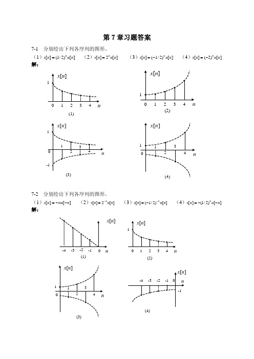
7-1 分别绘出下列各序列的图形。 (2)x[n] 2n u[n] (3)x[n] (1/ 2)n u[n] (4)x[n] (2) n u[ n] (1)x[n] (1/ 2)n u[n] 解:
x[ n ]
1
x[n]
1
0 1 2 (1) 3 4
n
0
1
2 3 (2)
x[n]
1
x[n]
-4
-3
-2 (1)
-1
0
n
0
1
2 (2)
3
4
n
x[n]
-4 1 0 1 2 3 4 -3 -2 -1 0
x[n] n
-1
n
(4)
(3)
7-3
分别绘出下列各序列的图形。 (2) x[n] cos
n 10 5
n (1) x[n] sin 5
1 z2 X (z) ( 1 1 2 z 1 )( 1 2 z 1 ) ( z 1 2 )( z 2 ) X (z) z 1 4 z ( z 1 2 )( z 2 ) 3( z 1 2 ) 3( z 2 )
X (z)
z 4z 3( z 1 2 ) 3 ( z 2 )
N
)
由于 x[n] 、 h[n] 均为因果序列,因此 y[n] 亦为因果序列,根据移位性质可求得
y [ n ] Z 1 [Y ( z )]
1 1 (1 a n 1 ) u [ n ] (1 a n 1 N ) u [ n N ] 1 a 1 a
7-24 计算下列序列的傅里叶变换。
(2)
奥本海姆《信号与系统》(第2版)知识点归纳考研复习(下册)

第7章采样第8章通信系统第9章拉普拉斯变换第10章Z变换第11章线性反馈系统第7章采样7.2连续时间信号x(t)从一个截止频率为的理想低通滤波器的输出得到,如果对x(t)完成冲激串采样,那么下列采样周期中的哪一些可能保证x(t)在利用一个合适的低通滤波器后能从它的样本中得到恢复?7.3在采样定理中,采样频率必须要超过的那个频率称为奈奎斯特率。
试确定下列各信号的奈奎斯特率:7.4设x(t)是一个奈奎斯特率为ω0的信号,试确定下列各信号的奈奎斯特率:7.5设x(t)是一个奈奎斯特率为ω0的信号,同时设其中。
7.6在如图7-1所示系统中,有两个时间函数x1(t)和x2(t)相乘,其乘积W (t)由一冲激串采样,x1(t)带限于ω17.7信号x(t)用采样周期T经过一个零阶保持的处理产生一个信号x0(t),设x1(t)是在x(t)的样本上经过一阶保持处理的结果,即7.8有一实值且为奇函数的周期信号x(t),它的傅里叶级数表示为7.9考虑信号x(t)为7.10判断下面每一种说法是否正确。
7.11设是一连续时间信号,它的傅里叶变换具有如下特点:7.12有一离散时间信号其傅里叶变换具有如下性质:7.13参照如图7-7所示的滤波方法,假定所用的采样周期为T,输入xc(t)为带限,而有7.14假定在上题中有重做习题7.13。
7.15对进行脉冲串采样,得到若7.16关于及其傅里叶变换7.17考虑理想离散时间带阻滤波器,其单位脉冲响应为频率响应在条件下为7.18假设截止频率为π/2的一个理想离散时间低通滤波器的单位脉冲响应是用于内插的,以得到一个2倍的增采样序列,求对应于这个增采样单位脉冲响应的频率响应。
7.19考虑如图7-11所示的系统,输入为x[n],输出为y[n]。
零值插入系统在每一序列x[n]值之间插入两个零值点,抽取系统定义为其中W[n]是抽取系统的输入序列。
若输入x[n]为试确定下列ω1值时的输出y[n]:7.20有两个离散时间系统S1和S2用于实现一个截止频率为π/4的理想低通滤波器。
奥本海姆《信号与系统》(第2版)课后习题-第7章至第9章(下册)(圣才出品)

第二部分课后习题第7章采样基本题7.1已知实值信号x(t),当采样频率时,x(t)能用它的样本值唯一确定。
问在什么ω值下保证为零?解:对于因其为实函数,故是偶函数。
由题意及采样定理知的最大角频率即当时,7.2连续时间信号x(t)从一个截止频率为的理想低通滤波器的输出得到,如果对x(t)完成冲激串采样,那么下列采样周期中的哪一些可能保证x(t)在利用一个合适的低通滤波器后能从它的样本中得到恢复?解:因为x(t)是某个截止频率的理想低通滤波器的输出信号,所以x(t)的最大频率就为=1000π,由采样定理知,若对其进行冲激采样且欲由其采样m点恢复出x(t),需采样频率即采样时间问隔从而有(a)和(c)两种采样时间间隔均能保证x(t)由其采样点恢复,而(b)不能。
7.3在采样定理中,采样频率必须要超过的那个频率称为奈奎斯特率。
试确定下列各信号的奈奎斯特率:解:(a)x(t)的频谱函数为由此可见故奈奎斯特频率为(b)x(t)的频谱函数为由此可见故奈奎斯特频率为(c)x(t)的频谱函数为由此可见,当故奈奎斯特频率为7.4设x(t)是一个奈奎斯特率为ω0的信号,试确定下列各信号的奈奎斯特率:解:(a)因为的傅里叶变换为可见x(t)的最大频率也是的最大频率,故的奈奎斯特频率为0 。
(b)因为的傅里叶变换为可见x (t)的最大频率也是的最大频率.故的奈奎斯特频率仍为。
(c)因为的傅里叶变换蔓可见的最大频率是x(t)的2倍。
从而知x 2(t)的奈奎斯特频率为2(d)因为的傅里叶变换为,x(t)的最大频率为,故的最大频率为,从而可推知其奈奎斯特频率为7.5设x(t)是一个奈奎斯特率为ω0的信号,同时设其中。
当某一滤波器以Y(t)为输入,x(t)为输出时,试给出该滤波器频率响应的模和相位特性上的限制。
解:p(t)是一冲激串,间隔对x(t)用p(t-1)进行冲激采样。
先分别求出P(t)和P(t-1)的频谱函数:注意0ω是x(t)的奈奎斯特频率,这意味着x(t)的最大频率为02ω,当以p(t-1)对x(t)进行采样时,频谱无混叠发生。
信号与系统_第二版_奥本海默 _课后答案[1-10章]
![信号与系统_第二版_奥本海默 _课后答案[1-10章]](https://img.taocdn.com/s3/m/6ff45c8f83c4bb4cf6ecd112.png)
学霸助手[]-课后答案|期末试卷|复习提纲
学霸h助us手 Contents baz Chapter 1 ······················································· 2 xue Chapter 2 ······················································· 17
e 5 = 5 j0 ,
e -2 = 2 ,jp
e -3 j = 3
-
j
p 2
e 1
2
-
j
3 2
=
, -
j
p 2
e 1+ j =
2
, j
p 4
( ) 1- j e 2 =2
-
j
p 2
ep
j(1- j) = 4 ,
e 1+
1-
j j
=
p 4
e 2 + j 2 = -1p2
1+ j 3
ò e 1.3.
(a)
xue学ba霸zh助usS手hoiug.ncoaml(Sseco&nd EdSitioyn)stems
—Learning Instructions
xu(eEbxe学arzc霸hisue助sshA手onus.wceorms)
Department
of
Computer 2005.12
Enginexeurein学bga霸zh助us手
=¥
E¥
0
-4tdt
=
1 4
,
P ¥ =0, because
E¥ < ¥
手 om ò (b)
x e , 2(t) = j(2t+p4 )
信号与系统(奥本海默第二版)第7章

(a) 脉冲抽样
First-order fold interpolation
|t | 1 sin(T / 2) h1 (t ) 1 , | t | T H1 ( j ) T T /2
2
x1 (t ) x p (t ) * h1 (t )
h1 (t ) * x(nT ) (t nT )
n
x(t ) (t nT )
x2(kT) x2(kT)
n
x(nT ) (t nT )
7.1.1 Impulse-train sampling
p(t)
N
x p (t )
(t nT)
In frequency domain
Band limited interpolation
cT sin(ct) 内插 h(t) ct 函数
xr (t ) x p (t ) * h(t ),
[ x(nT) (t nT)] * h(t)
n
n
[x(nT) (t nT)ቤተ መጻሕፍቲ ባይዱ* h(t)]
x0 (t ) h0 (t ) * x p (t )
n
x(nT)h (t nT)
0
Examples for the applications of zero-order fold interpolation (c )图(a)的1/4间隔抽样, (b)零级保持-重建 零级保持-重建
1 X d (e ) X c ( j ( / T 2k )) T k
1 2k X p ( j ) X ( ) T k T
《信号与系统》奥本海姆第七章

采样频率: 1 f s 2 f M 或 s 2M T
Generated by Foxit PDF Creator © Foxit Software For evaluation only.
信号重建:
x(t)
连续信号
∞
xp(t)
FT
x1 (t ) X1 ( j) 0,| | 1 ;
FT
x2 (t ) X 2 ( j) 0,| | 2 ;
[1 2 ]
计算 x(t ) x1 (t ) x2 (t ) 的采样频率.
20
Generated by Foxit PDF Creator © Foxit Software For evaluation only.
1 1 n 0时, X p j X j , 包 T 含原信号的全部信息, 幅度差T倍。
Xp( j)
A/ T
2
X p j 以s为周期的连续谱 , 有 新的频率成分 ,即 X j 的周期 性延拓。
s
0
s
A
X ( j)
s s M
M M
离散信号与系统的主要优点:
(1) 信号稳定性好 (2) 信号可靠性高 (3) 信号处理简便 (4) 系统灵活性强
4
Generated by Foxit PDF Creator © Foxit Software For evaluation only.
7.0 引言
采样定理是从连续信号到离散信号的桥梁, 也是对信号进行数字处理的第一个环节。
fs (t )
f (t )
A/ D
量化编码
f (n)
数字 滤波器
g(n)
奥本海姆《信号与系统》课件8

−ωs −ωM 0 ωMωcωs
仕 四. Nyquist 采样定理:
良
信号与系统
ω
对带限于最高频率 ωM 的连续时间信号 x(t),
如果以ωs ≥ 2ωM 的频率进行理想采样,则 x(t)可
以唯一的由其样本 x(nT )来确定。将
fs = 2 fm 1
Ts = 2 fm
奈奎斯特速率 奈奎斯特时间(间隔)
1. x(t) 必须是带限的,最高频率分量为 ωM 。
2. 采样间隔(周期)不能是任意的,必须保证采
样频率 ωs ≥ 2ωM 。其中ωs =2π /T为采样频率。
在满足上述要求时,可以通过理想低通滤波器
从 X p ( jω) 中不失真地分离出 X ( jω )。
Xp( jω)
1
主
TT
讲
教 师: 赵
为周期进行延拓(时域离散化,频域周期化)。
信号与系统
主 讲 教 师: 赵 仕 良
信号与系统
主
要想使采样后的信号样本能完全代表原来的信
讲
教 师:
号,就意味着要能够从 X p ( jω) 中不失真地分离
赵
仕 出 X ( jω ) 。这就要求 X p ( jω)在周期性延拓时不
良
能发生频谱的混叠。为此必须要求:
X ( jω) ∗ P( jω)
p (t )
三.冲激串采样(理想采样):
∞
p(t) = ∑ δ (t − nT)
T 为采样间隔
n = −∞ +∞
xp(t) = x(t) p(t) = x(t) ∑δ (t − nT )
+∞
n =−∞
= ∑ x(nT )δ (t − nT )
信号与系统 奥本海姆 第二版 习题详解

对方程两边同时做反变换得:
y[n] −
1 处有一个二阶极点,因为系统是因果的,所以 H ( z ) 的收敛域是 z > , (b)H ( z) 在 z = 1 3 3 包括单位圆,所以系统是稳定的。
解: (a) x[n] = δ [n + 5] ← → X ( z ) = z , ROC : 全部z 因为收敛域包括单位圆,所以傅立叶变换存在。
( )
χ (s ) = uL{e −2t u (t )} =
H (s ) =
H (s )如图所示。
Y (s ) 1 = 2 . X (s ) s − s − 2
1 1 1 3 3 ( ) , ⇒ H s = − s2 − s − 2 s − 2 s +1 (i )如果系统是稳定的,H (s )的ROC为 − 1〈ℜe {s}〈2.
∞ ∞
n =−∞
∑
∞
x[n]z − n =
− n−2
1 −n ∞ 1 n z = ∑− z ∑ −3 3 n =−∞ n =2
−2 n −n
z n + 2 = 9 z 2 /(1 + 3z ) = 3z /(1 + (1/ 3) z −1 ), z < 1 3 1 = ∑ n =2 3
1 1 (b) H (s) = 1 − 3 s − 2 s +1
(1)系统是稳定的,说明 H (s) 的收敛域应该包括虚轴在内,即: − 1 < Re{s} < 2 , 所以 h(t ) = 1 (− e u (−t ) − e u (t )) 3 (2)系统是因果的,则 H (s) 的收敛域应为 Re{s} > 2 ,所以 h(t ) = 1 (e u (t ) − e u (t )) 3 ( 3 ) 系 统 既 不 因 果 又 不 稳 定 , 则 H (s) 的 收 敛 域 应 为 Re{s} < −1 , 所 以
chapter 7信号与系统 奥本海默 华科 电信系 英文 课件
1/3 1/2
1 3/2
Re
z
1 2
Example 7.4 n 1 Consider the signal x[n] 3 sin 4 n u[n].
x[n]
The z-transform of this signal is n n 1 1 1 j / 4 1 1 j / 4 1 X ( z) 3 e z 2 j 3 e z 2 j n 0 n 0
7.1 THE Z-TRANSFORM
The z-transform of a general discrete-time signal x[n] is defined as
X ( z)
n
x[n]z n
where z is a complex variable.
z re j , Expressing the complex variable z in polar form as
Example 7.2 Determine the z-transform of
X ( z ) a nu[n 1]z n
n
x[n] a nu[n 1].
a z
n
1
n n
a z
n n 1
n
1 (a z )
1 1 j / 4 1 1 e u[n] e j / 4 u[n] 2j3 2j3
n
n
1 1 1 1 Im j / 4 1 2 j 1 1 e z 2 j 1 1 e j / 4 z 1 3 3
信号与系统课件(奥本海姆+第二版)+中文课件

●离散周期信号可表示为: x[n]=x[n+mN] , m=0,1,2,3,……
其中:N为正整数。 把能使上式成立的最小正整数N,称为x[n]的基波周期 N 0 。
x [n]
N0
-4
-1
2
5
-5 -3 -2 0 1 3 4 6
2)、不满足上述关系的信号则称为非周期信号。
nN0 = 3
3、奇信号与偶信号
1、若 0< a <1,则x(at)是将x(t)在时间轴线性展宽a倍。(使变化减慢)
例如:若取a=1/2,则得x(t/2) 。此时原函数x(t)中t=1 时的值,等于在 x(t/2)中 t =2的值,即x(2*1/2)= x (1)。如图(b)所示;
2、若 a >1 , 则x(at)是将x(t)在时间轴线性压缩a倍。(使变化加速)
∫t2
2
E∞
=
lim
T →∞
t1
x (t )
dt
∫ ,
P∞
= lim 1 T→∞ T
t2
2
x(t) dt
t1
1)、能量信号
信号的能量E满足: 0< E∞ <∞
,而
P∞
= lim E∞ T →∞ 2T
=0
2 )、功率信号
信号的平均功率P满足:0 < P∞ < ∞ ,而 E∞ = ∞
例1:已知信号为 x[n] = e jω0n,试问是能量信号还是功率信号。
一、时移(信号的平移)——即信号的波形沿x轴左右平行移动,但波的形状 不变。
1、设连续信号x(t)的波形如图(a)所示,今将x(t)沿t轴平移 t 0 ,即得到平移
信号x(t-
- 1、下载文档前请自行甄别文档内容的完整性,平台不提供额外的编辑、内容补充、找答案等附加服务。
- 2、"仅部分预览"的文档,不可在线预览部分如存在完整性等问题,可反馈申请退款(可完整预览的文档不适用该条件!)。
- 3、如文档侵犯您的权益,请联系客服反馈,我们会尽快为您处理(人工客服工作时间:9:00-18:30)。
X r ( j ) [ (s 0 )] e j [ (s 0 )] e j
xr (t ) cos[(s 0 )t ]
表明恢复的信号不仅频率降低,而且相位相反。
工程应用时,如果采样频率 s 2M 将不足
一.欠采样与频谱混叠: 如果采样时,不满足采样定理的要求,就一定会 在 x(t ) 的频谱周期延拓时,出现频谱混叠的现象。 此时,即使通过理想内插也得不到原信号。但是 无论怎样,恢复所得的信号 xr (t )与原信号 x(t ) 在采 样点上将具有相同的值。
xr (nT ) x(nT )
例: x(t ) cos 0t
x (nT ) (t nT)
c
xd (n) xc (nT )
1 2 在频域: X p ( j ) X c j ( ks ) , s T T k
X d (e j )
n
xc (nT )e jn(以 表示离散域频率)
X p ( j )
1 T
T
s M 0 M s
c
四. Nyquist 采样定理: 对带限于最高频率
M 的连续时间信号x(t ) ,
如果以 s 2M 的频率进行理想采样,则 x(t ) 可 以唯一的由其样本 x(nT ) 来确定。
• 在工程实际应用中,
理想滤波器是不可能实
n
表明:理想内插以理想低通滤波器的单位冲激 响应作为内插函数。
c Tc Sin ct Sin ct h(t ) Sinc( t ) T c t t
cT Sin c (t nT ) x(t ) x(nT ) c (t nT ) n
1 T
k
X ( j ( ks ))
2 s T
可见,在时域对连续时间信号进行理想采样,
就相当于在频域将连续时间信号的频谱以 s 为
周期进行延拓。
要想使采样后的信号样本能完全代表原来的信
号,就意味着要能够从 X p ( j ) 中不失真地分离
出 X ( j ) 。这就要求 X p ( j ) 在周期性延拓时不能
c c
yc (t )
y p (t )
n
y (n) (t nT )
Yd (e j )
n
Yp ( j )
n
y (n)e
d
j nT
yd (n)e jn
Yp ( j) Yd (e jT )
Yd (e
j
) Yp ( j ) T
T c
Sin c (t nT ) 时 x(t ) x(nT ) 当 c c (t nT ) n 2 T
s
这种内插称为时域中的带限内插。
二. 零阶保持内插: 零阶保持内插的内插函数是零阶保持系统的单 位冲激响应 h0 (t ) 。
| H0 ( j) |
现的。而非理想滤波器
一定有过渡带,因此,
实际采样时,
s 必须大
于 2 M 。
• 低通滤波器的截止频率必须满足: M c (s M ) • 为了补偿采样时频谱幅度的减小,滤波器应具
有 T 倍的通带增益。
三. 零阶保持采样:
(t )
延时T
h0 (t )
1
h0 (t )
X r ( j )
显然当 t nT 时有
xr (nT ) cos( s 0 )nT
cos s nT cos 0nT Sin s nT Sin 0nT
cos 0 nT x(nT )
s 2 / T
如果 x(t ) cos(0t ) ,则在上述情况下:
以从样本恢复原信号。
2 20 时 例如 x(t ) cos(0t ) 在 s T
x(t ) cos cos 0t sin 0t sin
x(nT ) cos cos 0nT
这和对 x1 (t ) cos cos 0t 采样的结果一样。 从用样本代替信号的角度出发,出现欠采样的
在日常生活中,常可以看到用离散时间信号表 示连续时间信号的例子。如传真的照片、电视屏幕 的画面、电影胶片等等,这些都表明连续时间信号 与离散时间信号之间存在着密切的联系。在一定条 件下,可以用离散时间信号代替连续时间信号而并 不丢失原来信号所包含的信息。
研究连续时间信号与离散时间信号之间的关系 主要包括 : 1. 在什么条件下,一个连续时间信号可以用它的 离散时间样本来代替而不致丢失原有的信息。 2. 如何从连续时间信号的离散时间样本不失真地 恢复成原来的连续时间信号。 3. 如何对一个连续时间信号进行离散时间处理。 4. 对离散时间信号如何进行采样、抽取及内插。
X p ( j )
n
xc (nT )e j nT
jT
T
X d (e ) X p ( j ) T
j
X p ( j ) Байду номын сангаасX d (e
)
1 1 j X d (e ) X c [ j ( 2 k )] T k T
可见,冲激串到序列的变换过程,在时域是一
可见,D/C转换是C/D转换的逆过程。
三. 连续时间信号的离散时间处理
p(t )
xc (t )
x p (t )
xd (n)
冲激串 到序列
j
yd (n)
Hd (e )
序列到 冲激串
y p (t )
yc (t )
C/D
D/C
xc (t )
Hc ( j )
yc (t )
假定 Hd (e j ) 1 ,有 yd (n) xd (n) ,在满足采 样定理时有 y p (t ) xp (t ) , yc (t ) xc (t ),整个系统是 恒等系统,表明D/C转换是C/D转换的逆系统。
发生频谱的混叠。为此必须要求:
1. x(t )必须是带限的,最高频率分量为 M 。 2. 采样间隔(周期)不能是任意的,必须保证采样 频率 s 2M 。其中s 2 / T 为采样频率。 在满足上述要求时,可以通过理想低通滤波器 从 X p ( j ) 中不失真地分离出 X ( j )。
TX ( j ) H (e
0
p d 即X c ( j ) H c ( j )
jT
s
情况是工程应用中不希望的。
二. 欠采样在工程实际中的应用
1. 采样示波器:
2. 频闪测速:
s
频闪器
0
旋转圆盘
1
2
3
4
s 40
s 20
4 s 0 3
s 0
7.4 连续时间信号的离散时间处理
对连续时间信号进行离散时间处理的系统可视 为三个环节的级连。
xc (t )
t
0
T
零阶保持系统
1. 零阶保持系统:是一个 h(t ) 为矩形脉冲的系统。
2. 零阶保持:信号的样本经零阶保持后,所得到
的信号是一个阶梯形信号。
x0 (t )
x(t )
x p (t )
p(t )
1
h0 (t )
t
x0 (t )
0 T
n
(t nT )
零阶保持采样相当于理想采样后,再级联一个
零阶保持系统。
为了能从 x0 (t ) 恢复 x(t ) ,就要求零阶保持后再 级联一个系统 H r ( j)。使得
H0 ( j ) H r ( j ) H ( j )
T , c
0, c
其中 M c s M 而 H 0 ( j )
2Sin T / 2) (
个对时间归一化的过程;在频域是一个频率去归一 化的过程。
X c ( j )
1
M 0 M
1 T
X p ( j )
s
M 0 M
s
X d (e j )
1 T
2
M T 0 M T
2
二. D/C 转换:
yd (n)
序列到 冲激串
d
y p (t )
TT
7.1 用样本表示连续时间信号: 采样定理
一. 采样
在某些离散的时间点上提取连续时间信号值的过 程称为采样。 是否任何信号都可以由它的离散时间样本来表示? 对一维连续时间信号采样的例子:
在没有任何条件限制的情况下,从连续时间信
号采样所得到的样本序列不能唯一地代表原来的
连续时间信号。
此外,对同一个连续时间信号,当采样间隔不 同时也会 得到不同的样本序列。
xd (n)
C/D
离散时间系统
H ( j )
yd (n)
D/C
yc (t )
xc (t )
yc (t )
一. C/D 转换: p(t )
xc (t )
x p (t )
冲激串 到序列
xd (n) xc (nT )
在时域: p(t )
n
(t nT)
n
x p (t ) xc (t ) p(t )
T 为采样间隔
x(t )
t
0
p(t )
2T
T
x(T )
t
0
T
2T
x p (t )
x(2T )
x(T ) x(2T ) x(0)
t
2T