数字信号处理实验第三版修改程序
北邮-DSP数字信号处理 实验-实验报告
北京邮电大学电子工程学院电子实验中心<数字信号处理实验>实验报告班级: xxx学院: xxx实验室: xxx 审阅教师:姓名(班内序号): xxx 学号: xxx 实验时间: xxx评定成绩:目录一、常规实验 (3)实验一常用指令实验 (3)1.试验现象 (3)2.程序代码 (3)3.工作原理 (3)实验二数据储存实验 (4)1.试验现象 (4)2.程序代码 (4)3.工作原理 (4)实验三I/O实验 (5)1.试验现象 (5)2.程序代码 (5)3.工作原理 (5)实验四定时器实验 (5)1.试验现象 (5)2.程序代码 (6)3.工作原理 (9)实验五INT2中断实验 (9)1.试验现象 (9)2.程序代码 (9)3.工作原理 (13)实验六A/D转换实验 (13)1.试验现象 (13)2.程序代码 (14)3.工作原理 (18)实验七D/A转换实验 (19)1.试验现象 (19)2.程序代码 (19)3.工作原理 (37)二、算法实验 (38)实验一快速傅里叶变换(FFT)算法实验 (38)1.试验现象 (38)2.程序代码 (38)3.工作原理 (42)实验二有限冲击响应滤波器(FIR)算法实验 (42)1.试验现象 (42)2.程序代码 (42)3.工作原理 (49)实验三无限冲击响应滤波器(IIR)算法实验 (49)1.试验现象 (49)2.程序代码 (49)3.工作原理 (56)作业设计高通滤波器 (56)1.设计思路 (56)2.程序代码 (57)3.试验现象 (64)一、常规实验实验一常用指令实验1.试验现象可以观察到实验箱CPLD右上方的D3按一定频率闪烁。
2.程序代码.mmregs.global _main_main:stm #3000h,spssbx xf ;将XF置1,D3熄灭call delay ;调用延时子程序,延时rsbx xf ;将XF置0,D3点亮call delay ;调用延时子程序,b _main ;程序跳转到"_MAIN"nopnop;延时子程序delay:stm 270fh,ar3 ;将0x270f(9999)存入ar3loop1:stm 0f9h,ar4 ;将0x0f9(249)存入ar4loop2:banz loop2,*ar4- ;*ar4自减1,不为0时跳到loop2的位置banz loop1,*ar3- ;*ar3自减1,不为0时跳到loop1的位置ret ;可选择延迟的返回nopnop.end3.工作原理主程序循环执行:D3熄灭→延时→D3点亮→延时。
数字信号处理第三版实验报告 (1)
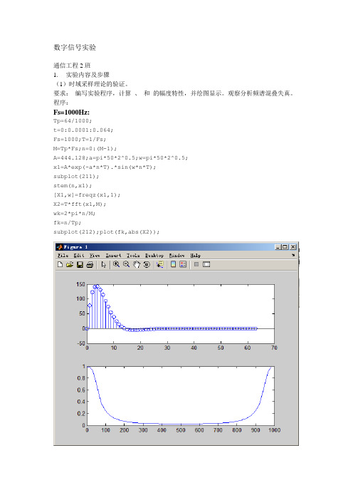
数字信号实验通信工程2班1. 实验内容及步骤(1)时域采样理论的验证。
要求:编写实验程序,计算、和的幅度特性,并绘图显示。
观察分析频谱混叠失真。
程序:Fs=1000Hz:Tp=64/1000;t=0:0.0001:0.064;Fs=1000;T=1/Fs;M=Tp*Fs;n=0:(M-1);A=444.128;a=pi*50*2^0.5;w=pi*50*2^0.5;x1=A*exp(-a*n*T).*sin(w*n*T);subplot(211);stem(n,x1);[X1,w]=freqz(x1,1);X2=T*fft(x1,M);wk=2*pi*n/M;fk=n/Tp;subplot(212);plot(fk,abs(X2));Fs=300Hz:Tp=64/1000;t=0:0.0001:0.064;Fs=300;T=1/Fs;N=Tp*Fs;n=0:N-1;A=444.128;a=pi*50*2^0.5;w=pi*50*2^0.5; x1=A*exp(-a*n*T).*sin(w*n*T);subplot(211);stem(n,x1);[X1,w]=freqz(x1,1);X2=T*fft(x1,N);wk=2*pi*n/N;fk=n/Tp;subplot(212);plot(fk,abs(X2));Fs=200Hz:Tp=64/1000;t=0:0.0001:0.064;Fs=200;T=1/Fs;N=Tp*Fs;n=0:N-1;A=444.128;a=pi*50*2^0.5;w=pi*50*2^0.5;x1=A*exp(-a*n*T).*sin(w*n*T);subplot(211);stem(n,x1);[X1,w]=freqz(x1,1);X2=T*fft(x1,N);wk=2*pi*n/N;fk=n/Tp;subplot(212);plot(fk,abs(X2));(2)频域采样理论的验证。
数字信号处理第三版(姚天任、江太辉) 答案 第三章
第三章离散傅里叶变换及其快速算法习题答案参考3.1 图P3.1所示的序列(xn 是周期为4的周期性序列。
请确定其傅里叶级数的系数(X k。
解:(111*0((((((N N N nk nk nk N N N n n n X k x n W x n W x n W X k X k −−−−−=====−= =−=∑∑∑3.2 (1设(xn 为实周期序列,证明(x n 的傅里叶级数(X k 是共轭对称的,即*((X k X k =− 。
(2证明当(xn 为实偶函数时,(X k 也是实偶函数。
证明:(1 111**((([(]((N nk N n N N nk nkNNn n Xk x n W Xk x n W xn W X−−=−−−==−=−===∑∑∑ k(2因(xn 为实函数,故由(1知有 *((Xk X k =− 或*((X k X k −= 又因(xn 为偶函数,即((x n x n =− ,所以有(111*0((((((N N N nk nk nk N N N n n n X k x n W x n W x n W X k X k −−−−−=====−= =−=∑∑∑3.3 图P3.3所示的是一个实数周期信号(xn 。
利用DFS 的特性及3.2题的结果,不直接计算其傅里叶级数的系数(Xk ,确定以下式子是否正确。
(1,对于所有的k; ((10Xk X k =+ (2((Xk X k =− ,对于所有的k; (3; (00X=(425(jkX k eπ,对所有的k是实函数。
解:(1正确。
因为(x n 一个周期为N =10的周期序列,故(X k 也是一个周期为N=10的周期序列。
(2不正确。
因为(xn 一个实数周期序列,由例3.2中的(1知,(X k 是共轭对称的,即应有*((Xk X = k −,这里(X k 不一定是实数序列。
(3正确。
因为(xn (0n ==在一个周期内正取样值的个数与负取样值的个数相等,所以有 10(0N n Xx −=∑ (4不正确。
数字信号处理实验报告_完整版
实验1 利用DFT 分析信号频谱一、实验目的1.加深对DFT 原理的理解。
2.应用DFT 分析信号的频谱。
3.深刻理解利用DFT 分析信号频谱的原理,分析实现过程中出现的现象及解决方法。
二、实验设备与环境 计算机、MATLAB 软件环境 三、实验基础理论1.DFT 与DTFT 的关系有限长序列 的离散时间傅里叶变换 在频率区间 的N 个等间隔分布的点 上的N 个取样值可以由下式表示:212/0()|()()01N jkn j Nk N k X e x n eX k k N πωωπ--====≤≤-∑由上式可知,序列 的N 点DFT ,实际上就是 序列的DTFT 在N 个等间隔频率点 上样本 。
2.利用DFT 求DTFT方法1:由恢复出的方法如下:由图2.1所示流程可知:101()()()N j j nkn j nN n n k X e x n eX k W e N ωωω∞∞----=-∞=-∞=⎡⎤==⎢⎥⎣⎦∑∑∑ 由上式可以得到:IDFTDTFT( )12()()()Nj k kX e X k Nωπφω==-∑ 其中为内插函数12sin(/2)()sin(/2)N j N x eN ωωφω--= 方法2:实际在MATLAB 计算中,上述插值运算不见得是最好的办法。
由于DFT 是DTFT 的取样值,其相邻两个频率样本点的间距为2π/N ,所以如果我们增加数据的长度N ,使得到的DFT 谱线就更加精细,其包络就越接近DTFT 的结果,这样就可以利用DFT 计算DTFT 。
如果没有更多的数据,可以通过补零来增加数据长度。
3.利用DFT 分析连续信号的频谱采用计算机分析连续时间信号的频谱,第一步就是把连续信号离散化,这里需要进行两个操作:一是采样,二是截断。
对于连续时间非周期信号,按采样间隔T 进行采样,阶段长度M ,那么:1()()()M j tj nT a a a n X j x t edt T x nT e ∞--Ω-Ω=-∞Ω==∑⎰对进行N 点频域采样,得到2120()|()()M jkn Na a M kn NTX j T x nT eTX k ππ--Ω==Ω==∑因此,可以将利用DFT 分析连续非周期信号频谱的步骤归纳如下: (1)确定时域采样间隔T ,得到离散序列(2)确定截取长度M ,得到M 点离散序列,这里为窗函数。
数字信号处理高西全实验报告三

数字信号处理高西全实验报告三选择FFT的变换区间N为8和16 两种情况进行频谱分析^p 。
分别打印其幅频特性曲线。
并进行对比、分析^p 和讨论。
(2)对以下周期序列进行谱分析^p 。
选择FFT的变换区间N为8和16 两种情况分别对以上序列进行频谱分析^p 。
分别打印其幅频特性曲线。
并进行对比、分析^p 和讨论。
(3)对模拟周期信号进行谱分析^p选择采样频率,变换区间N=16,32,64 三种情况进行谱分析^p 。
分别打印其幅频特性,并进行分析^p 和讨论。
四、程序码与运行结果(1) 实验程序:1n=[ones(1,4)];M=8;a=1:(M/2); b=(M/2):-1:1; 2n=[a,b];3n=[b,a];1k8=fft(1n,8);1k16=fft(1n,16);2k8=fft(2n,8);2k16=fft(2n,16);3k8=fft(3n,8);3k16=fft(3n,16);以下绘制幅频特性曲线n=0:length(1k8)-1;subplot(3,2,1);stem(n,abs(1k8),#;.#;);label({#;ω/π#;;#;8点DFT[1(n)]#;});ylabel(#;幅度#;);n=0:length(1k16)-1;subplot(3,2,2);stem(n,abs(1k16),#;.#;);label({#;ω/π#;;#;16点DFT[1(n)]#;});ylabel(#;幅度#;); n=0:length(2k8)-1;subplot(3,2,3);stem(n,abs(2k8),#;.#;);label({#;ω/π#;;#; 8点DFT[2(n)]#;});ylabel(#;幅度#;); n=0:length(2k16)-1;subplot(3,2,4);stem(n,abs(2k16),#;.#;);label({#;ω/π#;;#;16点DFT[2(n)]#;});ylabel(#;幅度#;); n=0:length(3k8)-1;subplot(3,2,5);stem(n,abs(3k8),#;.#;);l abel({#;ω/π#;;#; 8点DFT[3(n)]#;});ylabel(#;幅度#;); n=0:length(3k16)-1;subplot(3,2,6);stem(n,abs(3k16),#;.#;);label({#;ω/π#;;#;16点DFT[3(n)]#;});ylabel(#;幅度#;); 图形:(2)实验程序:n=0:7;4n=cos(pi/4n);4k8=fft(4n,8);subplot(2,2,1);stem(2n/8,abs(4k8),#;.#;);label({#;ω/π#;;#;8点DFT[4(n)]#;});ylabel(#;幅度#;); 5n=cos(pi/4n)+cos(pi/8n);5k8=fft(5n,8);subplot(2,2,2);stem(2n/8,abs(5k8),#;.#;);label({#;ω/π#;;#;8点DFT[5(n)]#;});ylabel(#;幅度#;); n=0:15;4n=cos(pi/4n);5n=cos(pi/4n)+cos(pi/8n);4k16=fft(4n,16);subplot(2,2,3);stem(2n/16,abs(4k16),#;.#;);label({#;ω/π#;;#;16点DFT[4(n)]#;});ylabel(#;幅度#;); 5k16=fft(5n,16);subplot(2,2,4);stem(2n/16,abs(5k16),#;.#;);label({#;ω/π#;;#;16点DFT[5(n)]#;});ylabel(#;幅度#;); 图形:(3)实验代码:Fs=64;T=1/Fs;N=16;n=0:N-1;6nT=cos(8pinT)+cos(16pinT)+cos(20pinT);6k16=fft(6nT);6k16=fftshift(6k16);Tp=NT;F=1/Tp;k=-N/2:N/2-1;fk=kF;subplot(3,1,1);stem(fk,abs(6k16),#;.#;);label({#;f(Hz)#;;#;16点DFT[6(nT)]#;});ylabel(#;幅度#;); N=32;n=0:N-1;6nT=cos(8pinT)+cos(16pinT)+cos(20pinT);6k32=fft(6nT,32);6k32=fftshift(6k32);Tp=NT;F=1/Tp;k=-N/2:N/2-1;fk=kF;subplot(3,1,2);stem(fk,abs(6k32),#;.#;);label({#;f(Hz)#;;#;32点DFT[6(nT)]#;});ylabel(#;幅度#;); N=64;n=0:N-1;6nT=cos(8pinT)+cos(16pinT)+cos(20pinT);6k64=fft(6nT,64);6k64=fftshift(6k64);Tp=NT;F=1/Tp;k=-N/2:N/2-1;fk=kF;subplot(3,1,3);stem(fk,abs(6k64),#;.#;);label({#;f(Hz)#;;#;64点DFT[6(nT)]#;});ylabel(#;幅度#;);图形:五、实验总结1.结论用DFT对信号进行谱分析^p 时,重点关注频谱分辨率和分析^p 误差,频谱分辨率F=1/Tp=Fs/N,可以依据此等式来选择FFT的变换区间N,而误差主要来自于用FFT作频谱分析^p 时,得到的是离散谱,而当信号是非周期信号时,应该得到连续谱,只有当N较大时,用FFT做出来的离散谱才接近于连续谱,因此N要适当选择大一些。
(完整版)数字信号处理实验三
3.41;3.42 由教材可知: ,即序列的偶部分的傅立叶变换是序列的傅立叶变换的实部。
5、实验步骤
1、进行本实验,首先必须熟悉matlab的运用,所以第一步是学会使用matlab。
2、学习相关基础知识,根据《数字信号处理》课程的学习理解实验内容和目的。
plot(w/pi,angle(h1));grid
xlabel('\omega/\pi');ylabel('以弧度为单位的相位');
title('原序列的相位谱')
subplot(2,2,4)
plot(w/pi,angle(h2));grid
xlabel('\omega/\pi');ylabel('以弧度为单位的相位');
grid;
title('相位谱arg[H(e^{j\omega})]');
xlabel('\omega/\pi');
ylabel('以弧度为单位的相位');
3.4
clf;
w=-4*pi:8*pi/511:4*pi;
num1=[1 3 5 7 9 11 13 15 17];
h=freqz(num,1,w);
Q3.32 通过加入合适的注释语句和程序语句,修改程序P3.8,对程序生成的图形中的两个轴加标记。时移量是多少?
Q3.33 运行修改后的程序并验证离散傅里叶变换的圆周时移性质。
Q3.36 运行程序P3.9并验证离散傅里叶变换的圆周卷积性质。
Q3.38 运行程序P3.10并验证线性卷积可通过圆周卷积得到。
数字信号处理(西电上机实验)
数字信号处理实验报告实验一:信号、系统及系统响应一、实验目的:(1) 熟悉连续信号经理想采样前后的频谱变化关系,加深对时域采样定理的理解。
(2) 熟悉时域离散系统的时域特性。
(3) 利用卷积方法观察分析系统的时域特性。
(4) 掌握序列傅里叶变换的计算机实现方法,利用序列的傅里叶变换对连续信号、离散信号及系统响应进行频域分析。
二、实验原理与方法:(1) 时域采样。
(2) LTI系统的输入输出关系。
三、实验内容、步骤(1) 认真复习采样理论、离散信号与系统、线性卷积、序列的傅里叶变换及性质等有关内容,阅读本实验原理与方法。
(2) 编制实验用主程序及相应子程序。
①信号产生子程序,用于产生实验中要用到的下列信号序列:a. xa(t)=A*e^-at *sin(Ω0t)u(t)A=444.128;a=50*sqrt(2)*pi;b. 单位脉冲序列:xb(n)=δ(n)c. 矩形序列:xc(n)=RN(n), N=10②系统单位脉冲响应序列产生子程序。
本实验要用到两种FIR系统。
a. ha(n)=R10(n);b. hb(n)=δ(n)+2.5δ(n-1)+2.5δ(n-2)+δ(n-3)③有限长序列线性卷积子程序用于完成两个给定长度的序列的卷积。
可以直接调用MATLAB语言中的卷积函数conv。
conv用于两个有限长度序列的卷积,它假定两个序列都从n=0 开始。
调用格式如下:y=conv (x, h)四、实验内容调通并运行实验程序,完成下述实验内容:①分析采样序列的特性。
a. 取采样频率fs=1 kHz, 即T=1 ms。
b. 改变采样频率,fs=300 Hz,观察|X(ejω)|的变化,并做记录(打印曲线);进一步降低采样频率,fs=200 Hz,观察频谱混叠是否明显存在,说明原因,并记录(打印)这时的|X(ejω)|曲线。
②时域离散信号、系统和系统响应分析。
a. 观察信号xb(n)和系统hb(n)的时域和频域特性;利用线性卷积求信号xb(n)通过系统hb(n)的响应y(n),比较所求响应y(n)和hb(n)的时域及频域特性,注意它们之间有无差别,绘图说明,并用所学理论解释所得结果。
(完整版)数字信号处理实验二

y = filter(num,den,x,ic);
yt = a*y1 + b*y2;
d = y - yt;
subplot(3,1,1)
stem(n,y);
ylabel('振幅');
title('加权输入: a \cdot x_{1}[n] + b \cdot x_{2}[n]的输出');
subplot(3,1,2)
%扫频信号通过2.1系统:
clf;
n = 0:100;
s1 = cos(2*pi*0.05*n);
s2 = cos(2*pi*0.47*n);
a = pi/2/100;
b = 0;
arg = a*n.*n + b*n;
x = cos(arg);
M = input('滤波器所需的长度=');
num = ones(1,M);
三、实验器材及软件
1.微型计算机1台
2. MATLAB 7.0软件
四、实验原理
1.三点平滑滤波器是一个线性时不变的有限冲激响应系统,将输出延时一个抽样周期,可得到三点平滑滤波器的因果表达式,生成的滤波器表示为
归纳上式可得
此式表示了一个因果M点平滑FIR滤波器。
2.对线性离散时间系统,若y1[n]和y2[n]分别是输入序列x1[n]和x2[n]的响应,则输入
plot(n, y);
axis([0, 100, -2, 2]);
xlabel('时间序号 n'); ylabel('振幅');
数字信号处理第三版用MATLAB上机实验
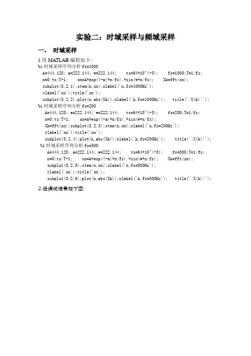
实验二:时域采样与频域采样一、时域采样1.用MATLAB编程如下:%1时域采样序列分析fs=1000A=444.128; a=222.144; w=222.144; ts=64*10^(-3); fs=1000;T=1/fs;n=0:ts/T-1; xn=A*exp((-a)*n/fs).*sin(w*n/fs); Xk=fft(xn);subplot(3,2,1);stem(n,xn);xlabel('n,fs=1000Hz');ylabel('xn');title('xn');subplot(3,2,2);plot(n,abs(Xk));xlabel('k,fs=1000Hz'); title('|X(k)|');%1时域采样序列分析fs=200A=444.128; a=222.144; w=222.144; ts=64*10^(-3); fs=200;T=1/fs;n=0:ts/T-1; xn=A*exp((-a)*n/fs).*sin(w*n/fs);Xk=fft(xn);subplot(3,2,3);stem(n,xn);xlabel('n,fs=200Hz'); ylabel('xn');title('xn');subplot(3,2,4);plot(n,abs(Xk));xlabel('k,fs=200Hz'); title('|X(k)|');%1时域采样序列分析fs=500A=444.128; a=222.144; w=222.144; ts=64*10^(-3); fs=500;T=1/fs;n=0:ts/T-1; xn=A*exp((-a)*n/fs).*sin(w*n/fs); Xk=fft(xn);subplot(3,2,5);stem(n,xn);xlabel('n,fs=500Hz');ylabel('xn');title('xn');subplot(3,2,6);plot(n,abs(Xk));xlabel('k,fs=500Hz'); title('|X(k)|');2.经调试结果如下图:20406080-200200n,fs=1000Hzxnxn2040608005001000k,fs=1000Hz|X (k)|51015-2000200n,fs=200Hzx nxn510150100200k,fs=200Hz |X(k)|10203040-2000200n,fs=500Hzx nxn102030400500k,fs=500Hz|X (k)|实验结果说明:对时域信号采样频率必须大于等于模拟信号频率的两倍以上,才 能使采样信号的频谱不产生混叠.fs=200Hz 时,采样信号的频谱产生了混叠,fs=500Hz 和fs=1000Hz 时,大于模拟信号频率的两倍以上,采样信号的频谱不产生混叠。
数字信号处理第三版高西全实验

数字信号处理第三版高西全实验数字信号处理第三版高西全实验》是一本旨在介绍数字信号处理的实际应用的教材。
本文档旨在概述该教材的目的和内容。
该教材的目的是通过实验教学的方式,帮助学生更好地理解数字信号处理的原理和技术,并将其应用到实际问题中。
它旨在培养学生的实践能力和解决问题的能力,使他们能够熟练地进行数字信号处理的实际操作。
该教材内容包括许多实验,涵盖了数字信号处理的各个方面。
每个实验都介绍了一个特定的概念或技术,并通过实际的操作和实验数据展示了其应用方式和效果。
学生通过完成实验,可以深入了解数字信号处理的各种算法和方法,研究如何使用相关工具和软件进行信号处理,以及如何分析和评估处理结果。
通过研究《数字信号处理第三版高西全实验》,学生将能够掌握数字信号处理的基本概念和技术,并能够独立地应用这些知识解决实际问题。
这将有助于他们在工程、通信、音视频处理等领域中的职业发展,也为进一步深入研究数字信号处理奠定了坚实的基础。
希望该教材能够对学生们的研究和实践有所帮助,使他们能够更好地理解和运用数字信号处理的方法和技术。
实验目标:本实验旨在介绍数字信号的采样和重构过程,并加深对这两个概念的理解。
实验目标:本实验旨在介绍数字信号的采样和重构过程,并加深对这两个概念的理解。
实验步骤:实验步骤:准备实验所需的信号发生器和示波器设备。
设置信号发生器,产生模拟信号,例如正弦波。
调整示波器参数,将模拟信号接入示波器进行显示。
使用采样器采样模拟信号,并记录采样得到的数字信号。
对采样得到的数字信号进行重构,恢复为原始模拟信号。
使用示波器将重构后的信号进行显示,并比较与原始信号的差异。
实验要点:了解采样和重构的基本概念和原理。
熟悉信号发生器和示波器的操作。
掌握采样器的使用方法。
理解数字信号与模拟信号的差异及其影响。
请参考实验指导书中的详细步骤和注意事项进行实验操作,并记录实验数据和结果。
本文档旨在解释《数字信号处理第三版高西全实验》中的实验二内容。
数字信号处理第三版_第一章
m 0
(n m )
3、矩形序列RN(n)
- Rectangular sequence
1 0 n N 1 RN ( n ) 0 其它n
RN(n)
1
…… …… 0 1 2 3 …… …… N-1
n
用单位阶跃序列u(n)表示矩形序列RN(n):
RN (n) u(n) u(n N )
y(n)
2 2 1 1
1
0
1 2 3 4 5 6
n
z(n)
2 2 2 2 1 0 1 2 3 4 5 6
n
3、序列的移位 :
y(n) = x(n±m)
设有一序列x(n),当m为正时: 右移 x(n-m)表示序列x(n)逐项依次右移m位后得到的序列。 左移 x(n+m)表示序列x(n)逐项依次左移m位后得到的序列。 x(n) x(0)=1 3 2 x(1)=2 1 1 x(2)=3 n
-4 -3 -2 -1 0 1 2 3 4 5 6 3
n
x(n)= (n) +2(n-1)+3(n-2)
2 1
m 0
x(m ) (n m )
2
(其中,x(0)=1, x(1)=2, x(2)=3)
-4 -3 -2 -1 0 1 2 3 4 5 6
n
2、单位阶跃序列u(n)
1 u( n) 0 u(n)
‘w1.wav’
x1(n)
0
1
2
3
4
5
6 x 10
7
4
1 0.8 0.6 0.4 0.2 0 -0.2 -0.4 -0.6 -0.8 -1
x2(n)
《数字信号处理》第三版课后习题答案
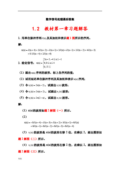
数字信号处理课后答案1.2 教材第一章习题解答1. 用单位脉冲序列()n δ及其加权和表示题1图所示的序列。
解:()(4)2(2)(1)2()(1)2(2)4(3) 0.5(4)2(6)x n n n n n n n n n n δδδδδδδδδ=+++-+++-+-+-+-+-2. 给定信号:25,41()6,040,n n x n n +-≤≤-⎧⎪=≤≤⎨⎪⎩其它(1)画出()x n 序列的波形,标上各序列的值;(2)试用延迟单位脉冲序列及其加权和表示()x n 序列; (3)令1()2(2)x n x n =-,试画出1()x n 波形; (4)令2()2(2)x n x n =+,试画出2()x n 波形; (5)令3()2(2)x n x n =-,试画出3()x n 波形。
解:(1)x(n)的波形如题2解图(一)所示。
(2)()3(4)(3)(2)3(1)6() 6(1)6(2)6(3)6(4)x n n n n n n n n n n δδδδδδδδδ=-+-+++++++-+-+-+-(3)1()x n 的波形是x(n)的波形右移2位,在乘以2,画出图形如题2解图(二)所示。
(4)2()x n 的波形是x(n)的波形左移2位,在乘以2,画出图形如题2解图(三)所示。
(5)画3()x n 时,先画x(-n)的波形,然后再右移2位,3()x n 波形如题2解图(四)所示。
3. 判断下面的序列是否是周期的,若是周期的,确定其周期。
(1)3()cos()78x n A n ππ=-,A 是常数;(2)1()8()j n x n e π-=。
解:(1)3214,73w w ππ==,这是有理数,因此是周期序列,周期是T=14; (2)12,168w wππ==,这是无理数,因此是非周期序列。
5. 设系统分别用下面的差分方程描述,()x n 与()y n 分别表示系统输入和输出,判断系统是否是线性非时变的。
北京理工大学 数字信号处理 实验报告 程序

数字信号处理实验报告1.深入掌握应用DFT分析信号的频谱的理论方法,针对该问题进行一次全面综合练习,完成一个完整的信号分析软件实现方法和流程,这种全面完整的综合练习可以帮助学生深入理解和消化基本理论,锻炼学生独立解决问题的能力,培养学生的创新意识,为今后的科研和工作打下良好的实践基础。
2.综合利用数字信号处理的理论知识完成数字滤波器的设计与实现,完成一个完整的数字滤波器设计软件的实现方法和流程。
这种全面完整的综合练习可以帮助学生深入理解和消化基本理论,锻炼学生独立解决问题的能力,培养学生的创新意识,为今后的科研和工作打下良好的实践基础。
二、实验设备与环境计算机、MATLAB软件环境三、实验内容1.基于Matlab GUI的离散傅里叶变换分析2.基于Matlab GUI的数字滤波器分析设计1.基于Matlab GUI的离散傅里叶变换分析信号: t=1:100;x=2*sin(t/25*2*pi)+5*sin(t/5*2*pi);说明:输入信号从Matlab Command Windows中生成,通过变量名导入本软件,并可输出DFT变换后的结果,默认名为DFT_输入变量名。
2.基于Matlab GUI的数字滤波器分析设计IIR 低通:(巴特沃兹)IIR高通:(切比雪夫I)IIR带通:(切比雪夫II)IIR带阻:(椭圆滤波器)FIR低通:(矩形窗)FIR高通:(汉宁窗)FIR带通:(布莱克曼窗)FIR带阻:(凯瑟窗)五、程序界面设计及程序源代码1.基于Matlab GUI的离散傅里叶变换分析界面设计:程序代码:function varargout =SignalDFTSoftware(varargin)% SIGNALDFTSOFTWARE MATLAB code for SignalDFTSoftware.fig% SIGNALDFTSOFTWARE, by itself, creates a new SIGNALDFTSOFTWARE or raises the existing% singleton*.%% H = SIGNALDFTSOFTWARE returns the handle to a new SIGNALDFTSOFTWARE or the handle to% the existing singleton*.%%SIGNALDFTSOFTWARE('CALLBACK',hObject,even tData,handles,...) calls the local% function named CALLBACK in SIGNALDFTSOFTWARE.M with the given input arguments.%%SIGNALDFTSOFTWARE('Property','Value',...) creates a new SIGNALDFTSOFTWARE or raises the% existing singleton*. Starting from the left, property value pairs are% applied to the GUI before SignalDFTSoftware_OpeningFcn gets called.An% unrecognized property name or invalid value makes property application% stop. All inputs are passed to SignalDFTSoftware_OpeningFcn via varargin. %% *See GUI Options on GUIDE's Tools menu. Choose "GUI allows only one% instance to run (singleton)".%% See also: GUIDE, GUIDATA, GUIHANDLES% Edit the above text to modify the response to help SignalDFTSoftware% Last Modified by GUIDE v2.5 26-Nov-2011 12:55:11% Begin initialization code - DO NOT EDITgui_Singleton = 1;gui_State = struct('gui_Name',mfilename, ...'gui_Singleton', gui_Singleton, ...'gui_OpeningFcn',@SignalDFTSoftware_OpeningFcn, ...'gui_OutputFcn',@SignalDFTSoftware_OutputFcn, ...'gui_LayoutFcn', [] , ...'gui_Callback', []);if nargin&&ischar(varargin{1})gui_State.gui_Callback = str2func(varargin{1}); endif nargout[varargout{1:nargout}] =gui_mainfcn(gui_State, varargin{:});elsegui_mainfcn(gui_State, varargin{:});end% End initialization code - DO NOT EDIT% --- Executes just before SignalDFTSoftware is made visible.function SignalDFTSoftware_OpeningFcn(hObjec t, eventdata, handles, varargin)% This function has no output args, see OutputFcn.% hObject handle to figure% eventdata reserved - to be defined in a future version of MATLAB% varargin command line arguments to SignalDFTSoftware (see VARARGIN)% Choose default command line output for SignalDFTSoftwarehandles.output = hObject;% Update handles structure guidata(hObject, handles);% UIWAIT makes SignalDFTSoftware wait for user response (see UIRESUME)% uiwait(handles.figure1);% --- Outputs from this function are returned to the command line.function varargout =SignalDFTSoftware_OutputFcn(hObject, eventdata, handles)% varargout cell array for returning output args (see VARARGOUT);% hObject handle to figure% eventdata reserved - to be defined in a future version of MATLAB% Get default command line output from handles structurevarargout{1} = handles.output;% --- If Enable == 'on', executes on mouse press in 5 pixel border.% --- Otherwise, executes on mouse press in 5 pixel border or over random.function random_ButtonDownFcn(hObject, eventdata, handles)% hObject handle to random (see GCBO)% eventdata reserved - to be defined in a future version of MATLAB% --- Executes on button press in random. function random_Callback(hObject, eventdata, handles)% hObject handle to random (see GCBO)% eventdata reserved - to be defined in a future version of MATLABglobal x;global x_flag;x=rand(1,50)*20-10;x_flag=1;if(x_flag)plot(handles.TD,0:(length(x)-1),x);end% --- Executes on button press in Delete.function Delete_Callback(hObject, eventdata, handles)% hObject handle to Delete (see GCBO)% eventdata reserved - to be defined in a future version of MATLABglobal x;global X;global x_flag;global X_flag;x=0;X=0;x_flag=0;X_flag=0;plot(handles.TD,0,0);plot(handles.FD,0,0);% --- If Enable == 'on', executes on mouse press in 5 pixel border.% --- Otherwise, executes on mouse press in 5 pixel border or over Delete.function Delete_ButtonDownFcn(hObject, eventdata, handles)% hObject handle to Delete (see GCBO)% eventdata reserved - to be defined in a future version of MATLAB% --- If Enable == 'on', executes on mouse press in 5 pixel border.% --- Otherwise, executes on mouse press in 5 pixel border or over Analyse.function Analyse_ButtonDownFcn(hObject, eventdata, handles)% hObject handle to Analyse (see GCBO)% eventdata reserved - to be defined in a future version of MATLAB% --- Executes on button press in Analyse. function Analyse_Callback(hObject, eventdata, handles)% hObject handle to Analyse (see GCBO)% eventdata reserved - to be defined in a future version of MATLAB global x;global X;global x_flag;global X_flag;if(x_flag)X=fft(x);X_flag=1;endif(X_flag)stem(handles.FD,linspace(0,2*pi,length(X)),abs( X));xlim(handles.FD,[0,2*pi])end% --- Executes on button press in Export. function Export_Callback(hObject, eventdata, handles)% hObject handle to Export (see GCBO)% eventdata reserved - to be defined in a future version of MATLABglobal X;global X_flag;if(X_flag)assignin('base',get(handles.edit4,'String'),X); end% --- Executes during object creation, after setting all properties.function text1_CreateFcn(hObject, eventdata, handles)% hObject handle to text1 (see GCBO)% eventdata reserved - to be defined in a future version of MATLAB% handles empty - handles not created until after all CreateFcns calledglobal x_flag;global X_flag;global x;global X;x_flag=0;X_flag=0;x=0;X=0;function name_Callback(hObject, eventdata, handles)% hObject handle to name (see GCBO)% eventdata reserved - to be defined in a future version of MATLAB% Hints: get(hObject,'String') returns contents of name as text% str2double(get(hObject,'String')) returns contents of name as a double% --- Executes during object creation, after setting all properties.function name_CreateFcn(hObject, eventdata, handles)if ispc&&isequal(get(hObject,'BackgroundColor'), get(0,'defaultUicontrolBackgroundColor')) set(hObject,'BackgroundColor','white'); end% --- Executes on button press in import. function import_Callback(hObject, eventdata, handles)global x;global x_flag;global signal_name;signal_name=get(,'String');x='empty';set(,'String','Notexist,Retry!');x=evalin('base',signal_name);set(,'String','Succeed');x_flag=1;if(x_flag)plot(handles.TD,0:(length(x)-1),x);endset(handles.edit4,'String',strcat('DFT_',signal_na me));function edit4_Callback(hObject, eventdata, handles)function edit4_CreateFcn(hObject, eventdata, handles)if ispc&&isequal(get(hObject,'BackgroundColor'), get(0,'defaultUicontrolBackgroundColor')) set(hObject,'BackgroundColor','white'); endglobal signal_name;2.基于Matlab GUI的数字滤波器分析设计界面设计:程序设计:function varargout = filter(varargin)%EDIT By Yu Yizhe%V1.0%2011/11/20%all right reserve% Begin initialization code - DO NOT EDITgui_Singleton = 1;gui_State = struct('gui_Name', mfilename, ...'gui_Singleton', gui_Singleton, ...'gui_OpeningFcn', @filter_OpeningFcn, ...'gui_OutputFcn', @filter_OutputFcn, ...'gui_LayoutFcn', [], ...'gui_Callback', []);if nargin&&ischar(varargin{1})gui_State.gui_Callback = str2func(varargin{1}); endif nargout[varargout{1:nargout}] =gui_mainfcn(gui_State, varargin{:});elsegui_mainfcn(gui_State, varargin{:});end% End initialization code - DO NOT EDIT% --- Executes just before filter is made visible. function filter_OpeningFcn(hObject, eventdata, handles, varargin)% This function has no output args, see OutputFcn.% hObject handle to figure% eventdata reserved - to be defined in a future version of MATLAB% varargin unrecognizedPropertyName/PropertyValue pairs from the% command line (see VARARGIN)% Choose default command line output for filter handles.output = hObject;% Update handles structureguidata(hObject, handles);% UIWAIT makes filter wait for user response (see UIRESUME)% uiwait(handles.figure1);% --- Outputs from this function are returned tothe command line.function varargout = filter_OutputFcn(hObject, eventdata, handles)% varargout cell array for returning output args (see VARARGOUT);% hObject handle to figure% eventdata reserved - to be defined in a future version of MATLAB% Get default command line output from handles structurevarargout{1} = handles.output;function text1_CreateFcn(hObject, eventdata, handles)global ch1;global ch2;global ch31;global ch32;ch1=1;ch2=1;ch31=1;ch32=1;function IIRtype_Callback(hObject, eventdata, handles)global ch1;global ch2;global ch31;global ch32;ch31=get(hObject,'Value');function IIRtype_CreateFcn(hObject, eventdata, handles)if ispc&&isequal(get(hObject,'BackgroundColor'), get(0,'defaultUicontrolBackgroundColor'))set(hObject,'BackgroundColor','white');endfunction e11_Callback(hObject, eventdata, handles)function e11_CreateFcn(hObject, eventdata, handles)if ispc&&isequal(get(hObject,'BackgroundColor'), get(0,'defaultUicontrolBackgroundColor')) set(hObject,'BackgroundColor','white'); endfunction e12_Callback(hObject, eventdata, handles)function e12_CreateFcn(hObject, eventdata, handles)if ispc&&isequal(get(hObject,'BackgroundColor'), get(0,'defaultUicontrolBackgroundColor')) set(hObject,'BackgroundColor','white'); endfunction e21_Callback(hObject, eventdata, handles)function e21_CreateFcn(hObject, eventdata, handles)if ispc&&isequal(get(hObject,'BackgroundColor'), get(0,'defaultUicontrolBackgroundColor')) set(hObject,'BackgroundColor','white'); endfunction e22_Callback(hObject, eventdata, handles)function e22_CreateFcn(hObject, eventdata, handles)if ispc&&isequal(get(hObject,'BackgroundColor'), get(0,'defaultUicontrolBackgroundColor')) set(hObject,'BackgroundColor','white'); endfunction e31_Callback(hObject, eventdata, handles)function e31_CreateFcn(hObject, eventdata, handles)if ispc&&isequal(get(hObject,'BackgroundColor'), get(0,'defaultUicontrolBackgroundColor')) set(hObject,'BackgroundColor','white'); endfunction e32_Callback(hObject, eventdata, handles)function e32_CreateFcn(hObject, eventdata, handles)if ispc&&isequal(get(hObject,'BackgroundColor'), get(0,'defaultUicontrolBackgroundColor')) set(hObject,'BackgroundColor','white'); endfunction e41_Callback(hObject, eventdata, handles)function e41_CreateFcn(hObject, eventdata, handles)if ispc&&isequal(get(hObject,'BackgroundColor'), get(0,'defaultUicontrolBackgroundColor')) set(hObject,'BackgroundColor','white'); endfunction e42_Callback(hObject, eventdata, handles)function e42_CreateFcn(hObject, eventdata, handles)if ispc&&isequal(get(hObject,'BackgroundColor'), get(0,'defaultUicontrolBackgroundColor')) set(hObject,'BackgroundColor','white'); endfunction generate_Callback(hObject, eventdata, handles)global ch1;global ch2;global ch31;global ch32;global typech;global w1p;global w1s;global w2p;global w2s;global rp;global rs;if ch1==1typech=ch1*100+ch2*10+ch31;elseif ch2==2typech=ch1*100+ch2*10+ch32;endw1p=str2num(get(handles.e11,'String'));w1s=str2num(get(handles.e12,'String'));w2p=str2num(get(handles.e21,'String'));w2s=str2num(get(handles.e22,'String'));rp=str2num(get(handles.e41,'String'));rs=str2num(get(handles.e42,'String')); Generate(handles);function FIRtype_Callback(hObject, eventdata, handles)global ch1;global ch2;global ch31;global ch32;ch32=get(hObject,'Value');function FIRtype_CreateFcn(hObject, eventdata, handles)if ispc&&isequal(get(hObject,'BackgroundColor'), get(0,'defaultUicontrolBackgroundColor')) set(hObject,'BackgroundColor','white'); endfunction poptype_Callback(hObject, eventdata, handles)global ch1;global ch2;global ch31;global ch32;ch2=get(hObject,'Value');reprint(handles);function poptype_CreateFcn(hObject, eventdata, handles)if ispc&&isequal(get(hObject,'BackgroundColor'), get(0,'defaultUicontrolBackgroundColor')) set(hObject,'BackgroundColor','white'); endfunction iirchoose_ButtonDownFcn(hObject, eventdata, handles)function firchoose_Callback(hObject, eventdata, handles)global ch1;global ch2;global ch31;global ch32;if(get(handles.firchoose,'Value')==0)set(handles.iirchoose,'Value',1);set(handles.FIRtype,'Visible','off');set(handles.IIRtype,'Visible','on');ch1=1;endif(get(handles.firchoose,'Value')==1)set(handles.iirchoose,'Value',0);set(handles.FIRtype,'Visible','on');set(handles.IIRtype,'Visible','off');ch1=2;endreprint(handles);function firchoose_ButtonDownFcn(hObject, eventdata, handles)function iirchoose_Callback(hObject, eventdata, handles)global ch1;global ch2;global ch31;global ch32;if(get(handles.iirchoose,'Value')==0)set(handles.firchoose,'Value',1);set(handles.FIRtype,'Visible','on');set(handles.IIRtype,'Visible','off');ch1=2;endif(get(handles.iirchoose,'Value')==1)set(handles.firchoose,'Value',0);set(handles.FIRtype,'Visible','off');set(handles.IIRtype,'Visible','on');ch1=1;endreprint(handles);function reprint(handles)global ch1;global ch2;global ch31;global ch32;temp=ch1*10+ch2;tempswitch tempcase {11,12}set(handles.add1,'Visible','off');set(handles.add2,'Visible','off');set(handles.e21,'Visible','off');set(handles.e22,'Visible','off');set(handles.pr,'Visible','on'); case{13,14}set(handles.add1,'Visible','on');set(handles.add2,'Visible','on');set(handles.e21,'Visible','on');set(handles.e22,'Visible','on');set(handles.pr,'Visible','on'); case{21,22},set(handles.add1,'Visible','off');set(handles.add2,'Visible','off');set(handles.e21,'Visible','off');set(handles.e22,'Visible','off');case{23,24},set(handles.add1,'Visible','on');set(handles.add2,'Visible','on');set(handles.e21,'Visible','on');set(handles.e22,'Visible','on');otherwisefprintf('switch error\n');endfunction Generate(handles)global ch1;global ch2;global ch31;global ch32;global typech;global w1p;global w1s;global w2p;global w2s;global rp;global rs;N=0;Wn=0;Wp=0;Wst=0;Rp=0;As=0;ftype='a';b=0;a=0;switch ch2case 1,ftype='low';case 2,ftype='high';case 3,ftype='bandpass';case 4,ftype='stop';endswitch ch2case {1,2}Wp=w1p;Wst=w1s;Rp=rp;As=rs;case {3,4}Wp=[w2p w1p];Wst=[w2s w1s];Rp=rp;As=rs;endswitch ch1 %IIR case 1,switch ch31case 1,[N,Wn]=buttord(Wp,Wst,Rp,As);[b,a]=butter(N,Wn,ftype); case 2,[N,Wn]=cheb1ord(Wp,Wst,Rp,As);[b,a]=cheby1(N,Rp,Wn,ftype);case 3,[N,Wn]=cheb2ord(Wp,Wst,Rp,As);[b,a]=cheby2(N,As,Wn,ftype); case 4,[N,Wn]=ellipord(Wp,Wst,Rp,As);[b,a]=ellip(N,Rp,As,Wn,ftype);endprint4(a,b,handles);case 2 %FIR tranbw=0;N=0;hw=0;Wn=(Wp+Wst)/2;switch ch32case 1, %Rectangular tranbw=1.8;N=ceil(tranbw/abs(w1s-w1p))+1;hw=boxcar(N);case 2, %Hanning tranbw=6.2;N=ceil(tranbw/abs(w1s-w1p))+1;hw=hanning(N);case 3, %Hamming tranbw=6.6;N=ceil(tranbw/abs(w1s-w1p))+1;hw=hamming(N);case 4, %Blackman tranbw=11;N=ceil(tranbw/abs(w1s-w1p))+1;hw=blackman(N);case 5, %KaiserN=(rs-7.95)/2.285/abs(w1s-w1p)+1;N=ceil(N);if (rs>=50)BTA=0.1102*(rs-8.7); elseif(rs>21)BTA=0.5842*(rs-21)^0.4+0.07886*(rs-21);elseBTA=0.5;endhw=kaiser(N,BTA);endh=fir1(N-1,Wn,ftype,hw');print4(h,N,handles);endfunction print4(a,b,handles)global ch1;if(ch1==1) %IIRw=[0:500]*pi/500;axes(handles.axes1);H=freqz(b,a,w);plot(handles.axes1,w/pi,abs(H)); xlabel('\Omega(\pi)');ylabel('|H(j\Omega)|');%axis ([0,0.5,0,1]);axes(handles.axes2);plot(handles.axes2,w/pi,20*log10((abs(H))/max(a bs(H))));xlabel('\Omega(\pi)');ylabel('|H(j\Omega)|,dB');% axis([0,0.5,-30,0]);axes(handles.axes3);plot(handles.axes3,w/pi,angle(H)/pi); xlabel('\Omega(\pi)');ylabel('Phase of H(j\Omega)(\pi)');%axis([0,0.5,-1,1]);t=0:30;axes(handles.axes4);h=impulse(b,a,t);stem(handles.axes4,t,h);xlabel('n');ylabel('Impulse Response');elseif(ch1==2) %FI RN=b;h=a;[H,w]=freqz(h,1);axes(handles.axes1);plot(handles.axes1,w/pi,abs(H)); xlabel('\Omega(\pi)');ylabel('|H(j\Omega)|');%axis ([0,0.5,0,1]);axes(handles.axes2);plot(handles.axes2,w/pi,20*log10((abs(H))/max(a bs(H))));xlabel('\Omega(\pi)');ylabel('|H(j\Omega)|,dB');% axis([0,0.5,-30,0]);axes(handles.axes3);plot(handles.axes3,w/pi,angle(H)/pi); xlabel('\Omega(\pi)');ylabel('Phase ofH(j\Omega)(\pi)');%axis([0,0.5,-1,1]);t=0:N-1;axes(handles.axes4);stem(handles.axes4,t,h);xlabel('n');ylabel('Impulse Response');end六、实验总结这次的数字信号处理实验非常有意义,让我学会了用计算机进行数字信号处理,计算各种参数,绘制出信号的波形,频谱。
数字信号处理 第三版 丁玉美
实验一 信号、系统及系统响应学号:1371031 姓名:来慧慧一、实验目的1. 掌握典型序列的产生方法。
2. 掌握DFT 的实现方法,利用DFT 对信号进行频域分析。
3. 熟悉连续信号经采样前后频谱的变化,加深对时域采样定理的理解。
4. 分别利用卷积和DFT 分析信号及系统的时域和频域特性,验证时域卷积定理。
二、实验环境1. Windows2000操作系统2. MATLAB6.0三、实验原理1. 信号采样对连续信号x a (t)=Ae -at sin(Ω0t)u(t)进行采样,采样周期为T,采样点0≤n<50,得采样序列x a (n)=。
2. 离散傅里叶变换(DFT)设序列为x(n),长度为N,则X(e j ωk )=DFT[x(n)]=∑-=10N n x(n) e -j ωk n ,其中ωk =k Mπ2(k=0,1,2,…,M-1),通常M>N,以便观察频谱的细节。
|X(e j ωk )|----x(n)的幅频谱。
4.连续信号采样前后频谱的变化^X a (j Ω)=)]([s m a m j X T 1Ω-Ω∑∞-∞= 即采样信号的频谱^X a (j Ω)是原连续信号x a (t)的频谱X a (j Ω)沿频率轴,以周期重复出现,幅度为原来的倍。
5. 采样定理由采样信号无失真地恢复原连续信号的条件,即采样定理为:。
6.时域卷积定理设离散线性时不变系统输入信号为x(n),单位脉冲响应为h(n),则输出信号y(n)=;由时域卷积定理,在频域中,Y(e j ω)=FT[y(n)]=。
四、实验内容1.分析采样序列特性(1)程序输入产生采样序列x a (n)= Ae -anT sin(Ω0nT)u(n)(0≤n<50),其中A=44.128,a=50π2,Ω0=50π2 采样频率f s (可变),T=1/f s 。
(要求写%程序注释)程序 shiyan11.mclear %clc %A=444.128;a=50*sqrt(2)*pi; %w0=50*sqrt(2)*pi;fs=input('输入采样频率fs=');T=1/fs;N=50;n=0:N-1;xa=A*exp(-a*n*T).*sin(w0*n*T); %subplot(221);stem(n,xa,'.');grid; %M=100;[Xa,wk]=DFT(xa,M); %f=wk*fs/(2*pi); %subplot(222);plot(f,abs(Xa));grid; %DFT 子函数:DFT.mfunction [X,wk]=DFT(x,M)N=length(x); %n=0:N-1;for k=0:M-1wk(k+1)=2*pi/M*k;X(k+1)=sum(x.*exp(-j*wk(k+1)*n)); %end(2)实验及结果分析a. 取fs=1000(Hz),绘出x a (n)及|Xa(e j ωk )|的波形。
数字信号处理(基于计算机的方法-第三版)matlab程序
% Program 2_1% Generation of the ensemble average%R = 50;m = 0:R-1;s = 2*m.*(0.9.^m); % Generate the uncorrupted signald = rand(R,1)-0.5; % Generate the random noisex1 = s+d';stem(m,d);xlabel('Time index n');ylabel('Amplitude'); title('Noise');pausefor n = 1:50;d = rand(R,1)-0.5;x = s + d';x1 = x1 + x;endx1 = x1/50;stem(m,x1);xlabel('Time index n');ylabel('Amplitude'); title('Ensemble average');% Program 2_2% Generation of complex exponential sequence%a = input('Type in real exponent = ');b = input('Type in imaginary exponent = ');c = a + b*i;K = input('Type in the gain constant = ');N = input ('Type in length of sequence = ');n = 1:N;x = K*exp(c*n);%Generate the sequencestem(n,real(x));%Plot the real partxlabel('Time index n');ylabel('Amplitude');title('Real part');disp('PRESS RETURN for imaginary part');pausestem(n,imag(x));%Plot the imaginary partxlabel('Time index n');ylabel('Amplitude');title('Imaginary part');% Program 2_3% Generation of real exponential sequence%a = input('Type in argument = ');K = input('Type in the gain constant = ');N = input ('Type in length of sequence = '); n = 0:N;x = K*a.^n;stem(n,x);xlabel('Time index n');ylabel('Amplitude'); title(['\alpha = ',num2str(a)]);% Program 2_4% Signal Smoothing by a Moving-Average Filter %R = 50;d = rand(R,1)-0.5;m = 0:1:R-1;s = 2*m.*(0.9.^m);x = s + d';plot(m,d,'r-',m,s,'b--',m,x,'g:')xlabel('Time index n'); ylabel('Amplitude') legend('d[n]','s[n]','x[n]');pauseM = input('Number of input samples = ');b = ones(M,1)/M;y = filter(b,1,x);plot(m,s,'r-',m,y,'b--')legend('s[n]','y[n]');xlabel ('Time index n');ylabel('Amplitude')% Program 2_5% Illustration of Median Filtering%N = input('Median Filter Length = ');R = 50; a = rand(1,R)-0.4;b = round(a); % Generate impulse noisem = 0:R-1;s = 2*m.*(0.9.^m); % Generate signalx = s + b; % Impulse noise corrupted signal y = medfilt1(x,3); % Median filteringsubplot(2,1,1)stem(m,x);axis([0 50 -1 8]);xlabel('n');ylabel('Amplitude');title('Impulse Noise Corrupted Signal');subplot(2,1,2)stem(m,y);xlabel('n');ylabel('Amplitude');title('Output of Median Filter');% Program 2_6% Illustration of Convolution%a = input('Type in the first sequence = ');b = input('Type in the second sequence = ');c = conv(a, b);M = length(c)-1;n = 0:1:M;disp('output sequence =');disp(c)stem(n,c)xlabel('Time index n'); ylabel('Amplitude');% Program 2_7% Computation of Cross-correlation Sequence%x = input('Type in the reference sequence = ');y = input('Type in the second sequence = ');% Compute the correlation sequencen1 = length(y)-1; n2 = length(x)-1;r = conv(x,fliplr(y));k = (-n1):n2';stem(k,r);xlabel('Lag index'); ylabel('Amplitude');v = axis;axis([-n1 n2 v(3:end)]);% Program 2_8% Computation of Autocorrelation of a% Noise Corrupted Sinusoidal Sequence%N = 96;n = 1:N;x = cos(pi*0.25*n); % Generate the sinusoidal sequenced = rand(1,N) - 0.5; % Generate the noise sequencey = x + d; % Generate the noise-corrupted sinusoidal sequence r = conv(y, fliplr(y)); % Compute the correlation sequencek = -28:28;stem(k, r(68:124));xlabel('Lag index'); ylabel('Amplitude');% Program 3_1% Discrete-Time Fourier Transform Computation%% Read in the desired number of frequency samplesk = input('Number of frequency points = ');% Read in the numerator and denominator coefficients num = input('Numerator coefficients = ');den = input('Denominator coefficients = ');% Compute the frequency responsew = 0:pi/(k-1):pi;h = freqz(num, den, w);% Plot the frequency responsesubplot(2,2,1)plot(w/pi,real(h));gridtitle('Real part')xlabel('\omega/\pi'); ylabel('Amplitude')subplot(2,2,2)plot(w/pi,imag(h));gridtitle('Imaginary part')xlabel('\omega/\pi'); ylabel('Amplitude')subplot(2,2,3)plot(w/pi,abs(h));gridtitle('Magnitude Spectrum')xlabel('\omega/\pi'); ylabel('Magnitude')subplot(2,2,4)plot(w/pi,angle(h));gridtitle('Phase Spectrum')xlabel('\omega/\pi'); ylabel('Phase, radians')% Program 3_2% Generate the filter coefficientsh1 = ones(1,5)/5; h2 = ones(1,14)/14;% Compute the frequency responses[H1,w] = freqz(h1, 1, 256);[H2,w] = freqz(h2, 1, 256);% Compute and plot the magnitude responsesm1 = abs(H1); m2 = abs(H2);plot(w/pi,m1,'r-',w/pi,m2,'b--');ylabel('Magnitude'); xlabel('\omega/\pi');legend('M=5','M=14');pause% Compute and plot the phase responsesph1 = angle(H1)*180/pi; ph2 = angle(H2)*180/pi;plot(w/pi,ph1,w/pi,ph2);ylabel('Phase, degrees');xlabel('\omega/\pi');legend('M=5','M=14');% Program 3_3% Set up the filter coefficientsb = [-6.76195 13.456335 -6.76195];% Set initial conditions to zero valueszi = [0 0];% Generate the two sinusoidal sequencesn = 0:99;x1 = cos(0.1*n);x2 = cos(0.4*n);% Generate the filter output sequencey = filter(b, 1, x1+x2, zi);% Plot the input and the output sequencesplot(n,y,'r-',n,x2,'b--',n,x1,'g-.');gridaxis([0 100 -1.2 4]);ylabel('Amplitude'); xlabel('Time index n');legend('y[n]','x2[n]','x1[n]')% Program 4_1% 4-th Order Analog Butterworth Lowpass Filter Design %format long% Determine zeros and poles[z,p,k] = buttap(4);disp('Poles are at');disp(p);% Determine transfer function coefficients[pz, pp] = zp2tf(z, p, k);% Print coefficients in descending powers of sdisp('Numerator polynomial'); disp(pz)disp('Denominator polynomial'); disp(real(pp))omega = [0: 0.01: 5];% Compute and plot frequency responseh = freqs(pz,pp,omega);plot (omega,20*log10(abs(h)));gridxlabel('Normalized frequency'); ylabel('Gain, dB');% Program 4_2% Program to Design Butterworth Lowpass Filter%% Type in the filter order and passband edge frequency N = input('Type in filter order = ');Wn = input('3-dB cutoff angular frequency = ');% Determine the transfer function[num,den] = butter(N,Wn,'s');% Compute and plot the frequency responseomega = [0: 200: 12000*pi];h = freqs(num,den,omega);plot (omega/(2*pi),20*log10(abs(h)));xlabel('Frequency, Hz'); ylabel('Gain, dB');% Program 4_3% Program to Design Type 1 Chebyshev Lowpass Filter%% Read in the filter order, passband edge frequency% and passband ripple in dBN = input('Order = ');Fp = input('Passband edge frequency in Hz = ');Rp = input('Passband ripple in dB = ');% Determine the coefficients of the transfer function [num,den] = cheby1(N,Rp,2*pi*Fp,'s');% Compute and plot the frequency responseomega = [0: 200: 12000*pi];h = freqs(num,den,omega);plot (omega/(2*pi),20*log10(abs(h)));xlabel('Frequency, Hz'); ylabel('Gain, dB');% Program 4_4% Program to Design Elliptic Lowpass Filter%% Read in the filter order, passband edge frequency, % passband ripple in dB and minimum stopband% attenuation in dBN = input('Order = ');Fp = input('Passband edge frequency in Hz = ');Rp = input('Passband ripple in dB = ');Rs = input('Minimum stopband attenuation in dB = '); % Determine the coefficients of the transfer function [num,den] = ellip(N,Rp,Rs,2*pi*Fp,'s');% Compute and plot the frequency responseomega = [0: 200: 12000*pi];h = freqs(num,den,omega);plot (omega/(2*pi),20*log10(abs(h)));xlabel('Frequency, Hz'); ylabel('Gain, dB');function y = circonv(x1, x2)% Develops a sequence y obtained by the circular% convolution of two equal-length sequences x1 and x2 L1 = length(x1);L2 = length(x2);if L1 ~= L2, error('Sequences of unequal length'), end y = zeros(1,L1);x2tr = [x2(1) x2(L2:-1:2)];for k = 1:L1,sh = circshift(x2tr', k-1)';h = x1.*sh;disp(sh);y(k) = sum(h);endfunction [Y] = haar_1D(X)% Computes the Haar transform of the input vector X% The length of X must be a power-of-2% Recursively builds the Haar matrix Hv = log2(length(X)) - 1;H = [1 1;1 -1];for m = 1:v,A = [kron(H,[1 1]);2^(m/2).*kron(eye(2^m),[1 -1])];H = A;endY = H*double(X(:));% Program 5_1% Illustration of DFT Computation%% Read in the length N of sequence and the desired% length M of the DFTN = input('Type in the length of the sequence = '); M = input('Type in the length of the DFT = ');% Generate the length-N time-domain sequenceu = [ones(1,N)];% Compute its M-point DFTU = fft(u,M);% Plot the time-domain sequence and its DFTt = 0:1:N-1;stem(t,u)title('Original time-domain sequence')xlabel('Time index n'); ylabel('Amplitude')pausesubplot(2,1,1)k = 0:1:M-1;stem(k,abs(U))title('Magnitude of the DFT samples')xlabel('Frequency index k'); ylabel('Magnitude') subplot(2,1,2)stem(k,angle(U))title('Phase of the DFT samples')xlabel('Frequency index k'); ylabel('Phase')% Program 5_2% Illustration of IDFT Computation%% Read in the length K of the DFT and the desired % length N of the IDFTK = input('Type in the length of the DFT = ');N = input('Type in the length of the IDFT = ');% Generate the length-K DFT sequencek = 0:K-1;V = k/K;% Compute its N-point IDFTv = ifft(V,N);% Plot the DFT and its IDFTstem(k,V)xlabel('Frequency index k'); ylabel('Amplitude') title('Original DFT samples')pausesubplot(2,1,1)n = 0:N-1;stem(n,real(v))title('Real part of the time-domain samples')xlabel('Time index n'); ylabel('Amplitude')subplot(2,1,2)stem(n,imag(v))title('Imaginary part of the time-domain samples')xlabel('Time index n'); ylabel('Amplitude')% Program 5_3% Numerical Computation of Fourier transform Using DFTk = 0:15; w = 0:511;x = cos(2*pi*k*3/16);% Generate the length-16 sinusoidal sequence X = fft(x); % Compute its 16-point DFTXE = fft(x,512); % Compute its 512-point DFT% Plot the frequency response and the 16-point DFT samplesplot(k/16,abs(X),'o', w/512,abs(XE))xlabel('\omega/\pi'); ylabel('Magnitude')% Program 5_4% Linear Convolution Via the DFT%% Read in the two sequencesx = input('Type in the first sequence = ');h = input('Type in the second sequence = ');% Determine the length of the result of convolutionL = length(x)+length(h)-1;% Compute the DFTs by zero-paddingXE = fft(x,L); HE = fft(h,L);% Determine the IDFT of the producty1 = ifft(XE.*HE);% Plot the sequence generated by DFT-based convolution and% the error from direct linear convolutionn = 0:L-1;subplot(2,1,1)stem(n,y1)xlabel('Time index n');ylabel('Amplitude');title('Result of DFT-based linear convolution')y2 = conv(x,h);error = y1-y2;subplot(2,1,2)stem(n,error)xlabel('Time index n');ylabel('Amplitude')title('Error sequence')% Program 5_5% Illustration of Overlap-Add Method%% Generate the noise sequenceR = 64;d = rand(R,1)-0.5;% Generate the uncorrupted sequence and add noisek = 0:R-1;s = 2*k.*(0.9.^k);x = s + d';% Read in the length of the moving average filterM = input('Length of moving average filter = ');% Generate the moving average filter coefficientsh = ones(1,M)/M;% Perform the overlap-add filtering operationy = fftfilt(h,x,4);% Plot the resultsplot(k,s,'r-',k,y,'b--')xlabel('Time index n');ylabel('Amplitude')legend('s[n]','y[n]')function Factors = factorize(polyn)format long; Factors = [];% Use threshold of 1e-8 instead of 0 to account for% precision effectsTHRESH = 1e-8;%proots = roots(polyn); % get the zeroes of the polynomiallen = length(proots); % get the number of zeroes%while(len > 1)if(abs(imag(proots(1))) < THRESH) % if the zero is a real zero fac = [1 -real(proots(1))];% construct the factor with proots(1) as zeroFactors = [Factors;[fac 0]];else % if the zero has imaginary part get all zeroes whose% imag part is -ve of imaginary part of proots(1)negimag = imag(proots)+imag(proots(1));% get all zeroes which have same real part as proot(1)samereal = real(proots)-real(proots(1));%find the complex conjugate zeroindex = find(abs(negimag) <THRESH & abs(samereal)<THRESH); if(index) % if the complex conjugate existsfac = [1 -2*real(proots(1)) abs(proots(1))^2];%form 2nd order factorFactors = [Factors;fac];else % if the complex conjugate does not existfac = [1 -proots(1)];Factors = [Factors;[fac 0]];endendpolyn = deconv(polyn,fac);%deconvolve the 1st/2nd order factor from polynproots = roots(polyn); %determine the new zeroslen = length(polyn); %determine the number of zerosend% Program 6_1% Determination of the Factored Form% of a Rational z-Transform%num = input('Type in the numerator coefficients = ');den = input('Type in the denominator coefficients = ');K = num(1)/den(1);Numfactors = factorize(num)Denfactors = factorize(den)disp('Numerator factors');disp(Numfactors);disp('Denominator factors');disp(Denfactors);disp('Gain constant');disp(K);zplane(num,den)% Program 6_2% Determination of the Rational z-Transform% from its Poles and Zeros%format longzr = input('Type in the zeros as a row vector = ');pr = input('Type in the poles as a row vector = ');% Transpose zero and pole row vectorsz = zr'; p = pr';k = input('Type in the gain constant = ');[num, den] = zp2tf(z, p, k);disp('Numerator polynomial coefficients'); disp(num);disp('Denominator polynomial coefficients'); disp(den);%Program 6_3% Partial-Fraction Expansion of Rational z-Transform%num = input('Type in numerator coefficients = ');den = input('Type in denominator coefficients = ');[r,p,k] = residuez(num,den);disp('Residues');disp(r')disp('Poles');disp(p')disp('Constants');disp(k)% Program 6_4% Partial-Fraction Expansion to Rational z-Transform%r = input('Type in the residues = ');p = input('Type in the poles = ');k = input('Type in the constants = ');[num, den] = residuez(r,p,k);disp('Numerator polynomial coefficients'); disp(num)disp('Denominator polynomial coefficients'); disp(den)% Program 6_5% Power Series Expansion of a Rational z-Transform%% Read in the number of inverse z-transform coefficients to be computed L = input('Type in the length of output vector = ');% Read in the numerator and denominator coefficients of% the z-transformnum = input('Type in the numerator coefficients = ');den = input('Type in the denominator coefficients = ');% Compute the desired number of inverse transform coefficients[y,t] = impz(num,den,L);disp('Coefficients of the power series expansion');disp(y')% Program 6_6% Power Series Expansion of a Rational z-Transform%% Read in the number of inverse z-transform coefficients% to be computedN = input('Type in the length of output vector = ');% Read in the numerator and denominator coefficients of % the z-transformnum = input('Type in the numerator coefficients = '); den = input('Type in the denominator coefficients = '); % Compute the desired number of inverse transform% coefficientsx = [1 zeros(1, N-1)];y = filter(num, den, x);disp('Coefficients of the power series expansion'); disp(y)%Program_6_7% Stability Test%num = input('Type in the numerator vector = ');den = input('Type in the denominator vector = ');N = max(length(num),length(den));x = 1; y0 = 0; S = 0;zi = zeros(1,N-1);for n = 1:1000[y,zf] = filter(num,den,x,zi);if abs(y) < 0.000001, break, endx = 0;S = S + abs(y);y0 = y;zi = zf;endif n < 1000disp('Stable Transfer Function');elsedisp('Unstable Transfer Function');end% Program 7_1% Illustration of Deconvolution%Y = input('Type in the convolved sequence = ');H = input('Type in the convolving sequence = ');[X,R] = deconv(Y,H);disp('Sequence x[n]');disp(X);disp('Remainder Sequence r[n]');disp(R);% Program 7_2% Stability Test of a Rational Transfer Function%% Read in the polynomial coefficientsden = input('Type in the denominator coefficients ='); % Generate the stability test parametersk = poly2rc(den);knew = fliplr(k');disp('The stability test parameters are');disp(knew); stable = all(abs(k) < 1)% Program 8_2% Factorization of a Rational IIR Transfer Function%format shortnum = input('Numerator coefficients = ');den = input('Denominator coefficients = '); Numfactors = factorize(num);Denfactors = factorize(den);disp('Numerator Factors'),disp(Numfactors)disp('Denominator Factors'),disp(Denfactors)% Program 8_3% Parallel Realizations of an IIR Transfer Function%num = input('Numerator coefficient vector = ');den = input('Denominator coefficient vector = ');[r1,p1,k1] = residuez(num,den);[r2,p2,k2] = residue(num,den);disp('Parallel Form I')disp('Residues are');disp(r1);disp('Poles are at');disp(p1);disp('Constant value');disp(k1);disp('Parallel Form II')disp('Residues are');disp(r2);disp('Poles are at');disp(p2);disp('Constant value');disp(k2);% Program 8_4% Cascaded Lattice Realization of an% Allpass Transfer Function%format longden = input('Denominator coefficient vector = ');k = poly2rc(den);knew = fliplr(k);disp('The lattice section multipliers are');disp(knew');% Program 8_5% Realization of Gray-Markel Cascaded Lattice Structure %% den is the denominator coefficient vector% num is the numerator coefficient vector% k is the lattice parameter vector% alpha is the vector of feedforward multipliers%format long% Read in the transfer function coefficientsnum = input('Numerator coefficient vector = ');den = input('Denominator coefficient vector = ');num = num/den(1);den = den/den(1);[k,alpha] = tf2latc(num,den);disp('Lattice parameters are');disp(k');disp('Feedforward multipliers are');disp(fliplr(alpha'));% Program 8_6% Transfer Function of Gray-Markel Cascaded% Lattice Structure from the Lattice and% Feedforward Parameters% k1 is the lattice parameter vector% alpha is the vector of feedforward multipliers% den is the denominator coefficient vector% num is the numerator coefficient vector%format long% Read in the lattice and feedforward parametersk1 = input('Lattice parameter vector = ');alpha = input('Feedforward parameter vector = '); [num,den] = latc2tf(k1,fliplr(alpha));disp('Numerator coefficients are');disp(num)disp('Denominator coefficients are');disp(den)% Program 9_1% Elliptic IIR Lowpass Filter Design%Wp = input('Normalized passband edge = ');Ws = input('Normalized stopband edge = ');Rp = input('Passband ripple in dB = ');Rs = input('Minimum stopband attenuation in dB = '); [N,Wn] = ellipord(Wp,Ws,Rp,Rs)[b,a] = ellip(N,Rp,Rs,Wn);[h,omega] = freqz(b,a,256);plot (omega/pi,20*log10(abs(h)));grid;xlabel('\omega/\pi'); ylabel('Gain, dB');title('IIR Elliptic Lowpass Filter');% Program 9_2% Type 1 Chebyshev IIR Highpass Filter Design%Wp = input('Normalized passband edge = ');Ws = input('Normalized stopband edge = ');Rp = input('Passband ripple in dB = ');Rs = input('Minimum stopband attenuation in dB = '); [N,Wn] = cheb1ord(Wp,Ws,Rp,Rs);[b,a] = cheby1(N,Rp,Wn,'high');[h,omega] = freqz(b,a,256);plot (omega/pi,20*log10(abs(h)));grid;xlabel('\omega/\pi'); ylabel('Gain, dB');title('Type I Chebyshev Highpass Filter');% Program 9_3% Design of IIR Butterworth Bandpass Filter%Wp = input('Passband edge frequencies = ');Ws = input('Stopband edge frequencies = ');Rp = input('Passband ripple in dB = ');Rs = input('Minimum stopband attenuation = ');[N,Wn] = buttord(Wp, Ws, Rp, Rs);[b,a] = butter(N,Wn);[h,omega] = freqz(b,a,256);gain = 20*log10(abs(h));plot (omega/pi,gain);grid;xlabel('\omega/\pi'); ylabel('Gain, dB');title('IIR Butterworth Bandpass Filter');% Program 9_4% Group-delay equalization of an IIR filter.%[n,d] = ellip(4,1,35,0.3);[GdH,w] = grpdelay(n,d,512);plot(w/pi,GdH); gridxlabel('\omega/\pi'); ylabel('Group delay, samples'); title('Original Filter');pauseF = 0:0.001:0.3;g = grpdelay(n,d,F,2); % Equalize the passbandGd = max(g)-g;% Design the allpass delay equalizer[num,den,tau] = iirgrpdelay(8, F, [0 0.3], Gd); [GdA,w] = grpdelay(num,den,512);plot(w/pi,GdH+GdA); gridxlabel('\omega/\pi');ylabel('Group delay, samples'); title('Group Delay Equalized Filter');(注:可编辑下载,若有不当之处,请指正,谢谢!)。
数字信号处理实验第三版修改程序
实验一close all;clear all%======内容1:调用filter解差分方程,由系统对u(n)的响应判断稳定性====== A=[1,-0.9];B=[0.05,0.05]; %系统差分方程系数向量B和Ax1n=[1 1 1 1 1 1 1 1 zeros(1,50)]; %产生信号x1(n)=R8(n)x2n=ones(1,128); %产生信号x2(n)=u(n)hn=impz(B,A,58); %求系统单位脉冲响应h(n)subplot(2,2,1);stem(hn,'.'); %调用函数tstem绘图title('(a) 系统单位脉冲响应h(n)');box ony1n=filter(B,A,x1n); %求系统对x1(n)的响应y1(n)subplot(2,2,2);stem(y1n,'.');title('(b) 系统对R8(n)的响应y1(n)');box ony2n=filter(B,A,x2n); %求系统对x2(n)的响应y2(n)subplot(2,2,4);;stem(y2n,'.');title('(c) 系统对u(n)的响应y2(n)');box on%===内容2:调用conv函数计算卷积============================n=0:19x1n=[1 1 1 1 1 1 1 1 ]; %产生信号x1(n)=R8(n)h1n=[ones(1,10) zeros(1,10)];h2n=[1 2.5 2.5 1 zeros(1,10)];y21n=conv(h1n,x1n);y22n=conv(h2n,x1n);figure(2)subplot(2,2,1);;stem(n,h1n,'.'); %调用函数tstem绘图title('(d) 系统单位脉冲响应h1(n)');box onsubplot(2,2,2);stem([0:length(y21n)-1],y21n,'.');title('(e) h1(n)与R8(n)的卷积y21(n)');box onsubplot(2,2,3);stem([0:length(h2n)-1],h2n,'.'); %调用函数tstem绘图title('(f) 系统单位脉冲响应h2(n)');box onsubplot(2,2,4);stem([0:length(y22n)-1],y22n,'.');title('(g) h2(n)与R8(n)的卷积y22(n)');box on%=========内容3:谐振器分析========================un=ones(1,256); %产生信号u(n)n=0:255;xsin=sin(0.014*n)+sin(0.4*n); %产生正弦信号A=[1,-1.8237,0.9801];B=[1/100.49,0,-1/100.49]; %系统差分方程系数向量B和Ay31n=filter(B,A,un); %谐振器对u(n)的响应y31(n)y32n=filter(B,A,xsin); %谐振器对u(n)的响应y31(n)figure(3)subplot(2,1,1);stem(y31n,'.');title('(h) 谐振器对u(n)的响应y31(n)');box onsubplot(2,1,2);stem(y32n,'.');title('(i) 谐振器对正弦信号的响应y32(n)');box on实验二% 时域采样理论验证程序exp2a.mTp=64/1000; %观察时间Tp=64微秒%产生M长采样序列x(n)% Fs=1000;T=1/Fs;Fs=1000;T=1/Fs;M=Tp*Fs;n=0:M-1;A=444.128;alph=pi*50*2^0.5;omega=pi*50*2^0.5;xnt=A*exp(-alph*n*T).*sin(omega*n*T);Xk=T*fft(xnt,M); %M点FFT[xnt)]subplot(3,2,1);stem(xnt,'.'); %调用自编绘图函数tstem绘制序列图box on;title('(a) Fs=1000Hz');k=0:M-1;fk=k/Tp;subplot(3,2,2);plot(fk,abs(Xk));title('(a) T*FT[xa(nT)],Fs=1000Hz'); xlabel('f(Hz)');ylabel('幅度');axis([0,Fs,0,1.2*max(abs(Xk))])% 时域采样理论验证程序exp2a.mTp=64/1000; %观察时间Tp=64微秒%产生M长采样序列x(n)% Fs=1000;T=1/Fs;Fs=300;T=1/Fs;M=Tp*Fs;n=0:M-1;A=444.128;alph=pi*50*2^0.5;omega=pi*50*2^0.5;xnt=A*exp(-alph*n*T).*sin(omega*n*T);Xk=T*fft(xnt,M); %M点FFT[xnt)]subplot(3,2,3);stem(xnt,'.'); %调用自编绘图函数tstem绘制序列图box on;title('(a) Fs=300Hz');k=0:M-1;fk=k/Tp;subplot(3,2,4);plot(fk,abs(Xk));title('(a) T*FT[xa(nT)],Fs=300Hz'); xlabel('f(Hz)');ylabel('幅度');axis([0,Fs,0,1.2*max(abs(Xk))])% 时域采样理论验证程序exp2a.mTp=64/1000; %观察时间Tp=64微秒%产生M长采样序列x(n)% Fs=1000;T=1/Fs;Fs=300;T=1/Fs;M=Tp*Fs;n=0:M-1;A=444.128;alph=pi*50*2^0.5;omega=pi*50*2^0.5;xnt=A*exp(-alph*n*T).*sin(omega*n*T);Xk=T*fft(xnt,M); %M点FFT[xnt)]subplot(3,2,5);stem(xnt,'.'); %调用自编绘图函数tstem绘制序列图box on;title('(a) Fs=200Hz');k=0:M-1;fk=k/Tp;subplot(3,2,6);plot(fk,abs(Xk));title('(a) T*FT[xa(nT)],Fs=200Hz');xlabel('f(Hz)');ylabel('幅度');axis([0,Fs,0,1.2*max(abs(Xk))])%频域采样理论验证程序exp2b.mM=27;N=32;n=0:M;%产生M长三角波序列x(n)xa=0:floor(M/2); xb= ceil(M/2)-1:-1:0; xn=[xa,xb];Xk=fft(xn,1024); %1024点FFT[x(n)], 用于近似序列x(n)的TFX32k=fft(xn,32) ;%32点FFT[x(n)]x32n=ifft(X32k); %32点IFFT[X32(k)]得到x32(n)X16k=X32k(1:2:N); %隔点抽取X32k得到X16(K)x16n=ifft(X16k,N/2); %16点IFFT[X16(k)]得到x16(n)subplot(3,2,2);stem(n,xn,'.');box ontitle('(b) 三角波序列x(n)');xlabel('n');ylabel('x(n)');axis([0,32,0,20])k=0:1023;wk=2*k/1024; %subplot(3,2,1);plot(wk,abs(Xk));title('(a)FT[x(n)]');xlabel('\omega/\pi');ylabel('|X(e^j^\omega)|');axis([0,1,0,200])k=0:N/2-1;subplot(3,2,3);stem(k,abs(X16k),'.');box ontitle('(c) 16点频域采样');xlabel('k');ylabel('|X_1_6(k)|');axis([0,8,0,200])n1=0:N/2-1;subplot(3,2,4);stem(n1,x16n,'.');box ontitle('(d) 16点IDFT[X_1_6(k)]');xlabel('n');ylabel('x_1_6(n)');axis([0,32,0,20])k=0:N-1;subplot(3,2,5);stem(k,abs(X32k),'.');box ontitle('(e) 32点频域采样');xlabel('k');ylabel('|X_3_2(k)|');axis([0,16,0,200])n1=0:N-1;subplot(3,2,6);stem(n1,x32n,'.');box ontitle('(f) 32点IDFT[X_3_2(k)]');xlabel('n');ylabel('x_3_2(n)');axis([0,32,0,20])实验三clear all;close all%实验内容(1)===================================================x1n=[ones(1,4)]; %产生序列向量x1(n)=R4(n)M=8;xa=1:(M/2); xb=(M/2):-1:1; x2n=[xa,xb]; %产生长度为8的三角波序列x2(n) x3n=[xb,xa];X1k8=fft(x1n,8); %计算x1n的8点DFTX1k16=fft(x1n,16); %计算x1n的16点DFTX2k8=fft(x2n,8); %计算x1n的8点DFTX2k16=fft(x2n,16); %计算x1n的16点DFTX3k8=fft(x3n,8); %计算x1n的8点DFTX3k16=fft(x3n,16); %计算x1n的16点DFT%以下绘制幅频特性曲线subplot(2,2,1);stem(abs(X1k8),'.'); %绘制8点DFT的幅频特性图title('(1a) 8点DFT[x_1(n)]');xlabel('ω/π');ylabel('幅度');subplot(2,2,3);stem(abs(X1k16),'.'); %绘制16点DFT的幅频特性图title('(1b)16点DFT[x_1(n)]');xlabel('ω/π');ylabel('幅度');figure(2)subplot(2,2,1);stem(abs(X2k8),'.'); %绘制8点DFT的幅频特性图title('(2a) 8点DFT[x_2(n)]');xlabel('ω/π');ylabel('幅度');subplot(2,2,2);stem(abs(X2k16),'.'); %绘制16点DFT的幅频特性图title('(2b)16点DFT[x_2(n)]');xlabel('ω/π');ylabel('幅度');subplot(2,2,3);stem(abs(X3k8),'.'); %绘制8点DFT的幅频特性图title('(3a) 8点DFT[x_3(n)]');xlabel('ω/π');ylabel('幅度');subplot(2,2,4);stem(abs(X3k16),'.'); %绘制16点DFT的幅频特性图title('(3b)16点DFT[x_3(n)]');xlabel('ω/π');ylabel('幅度');%实验内容(2) 周期序列谱分析================================== N=8;n=0:N-1; %FFT的变换区间N=8x4n=cos(pi*n/4);x5n=cos(pi*n/4)+cos(pi*n/8);X4k8=fft(x4n); %计算x4n的8点DFTX5k8=fft(x5n); %计算x5n的8点DFTN=16;n=0:N-1; %FFT的变换区间N=16x4n=cos(pi*n/4);x5n=cos(pi*n/4)+cos(pi*n/8);X4k16=fft(x4n); %计算x4n的16点DFTX5k16=fft(x5n); %计算x5n的16点DFTfigure(3)subplot(2,2,1);stem(abs(X4k8),'.'); %绘制8点DFT的幅频特性图title('(4a) 8点DFT[x_4(n)]');xlabel('ω/π');ylabel('幅度');subplot(2,2,3);stem(abs(X4k16),'.'); %绘制16点DFT的幅频特性图title('(4b)16点DFT[x_4(n)]');xlabel('ω/π');ylabel('幅度');subplot(2,2,2);stem(abs(X5k8),'.'); %绘制8点DFT的幅频特性图title('(5a) 8点DFT[x_5(n)]');xlabel('ω/π');ylabel('幅度');subplot(2,2,4);stem(abs(X5k16),'.'); %绘制16点DFT的幅频特性图title('(5b)16点DFT[x_5(n)]');xlabel('ω/π');ylabel('幅度');%实验内容(3) 模拟周期信号谱分析===============================figure(4)Fs=64;T=1/Fs;N=16;n=0:N-1; %FFT的变换区间N=16x6nT=cos(8*pi*n*T)+cos(16*pi*n*T)+cos(20*pi*n*T); %对x6(t)16点采样X6k16=fft(x6nT); %计算x6nT的16点DFTX6k16=fftshift(X6k16); %将零频率移到频谱中心Tp=N*T;F=1/Tp; %频率分辨率Fk=-N/2:N/2-1;fk=k*F; %产生16点DFT对应的采样点频率(以零频率为中心)subplot(3,1,1);stem(fk,abs(X6k16),'.');box on %绘制8点DFT的幅频特性图title('(6a) 16点|DFT[x_6(nT)]|');xlabel('f(Hz)');ylabel('幅度');axis([-N*F/2-1,N*F/2-1,0,1.2*max(abs(X6k16))])N=32;n=0:N-1; %FFT的变换区间N=16x6nT=cos(8*pi*n*T)+cos(16*pi*n*T)+cos(20*pi*n*T); %对x6(t)32点采样X6k32=fft(x6nT); %计算x6nT的32点DFTX6k32=fftshift(X6k32); %将零频率移到频谱中心Tp=N*T;F=1/Tp; %频率分辨率Fk=-N/2:N/2-1;fk=k*F; %产生16点DFT对应的采样点频率(以零频率为中心)subplot(3,1,2);stem(fk,abs(X6k32),'.');box on %绘制8点DFT的幅频特性图title('(6b) 32点|DFT[x_6(nT)]|');xlabel('f(Hz)');ylabel('幅度');axis([-N*F/2-1,N*F/2-1,0,1.2*max(abs(X6k32))])N=64;n=0:N-1; %FFT的变换区间N=16x6nT=cos(8*pi*n*T)+cos(16*pi*n*T)+cos(20*pi*n*T); %对x6(t)64点采样X6k64=fft(x6nT); %计算x6nT的64点DFTX6k64=fftshift(X6k64); %将零频率移到频谱中心Tp=N*T;F=1/Tp; %频率分辨率Fk=-N/2:N/2-1;fk=k*F; %产生16点DFT对应的采样点频率(以零频率为中心)subplot(3,1,3);stem(fk,abs(X6k64),'.'); box on%绘制8点DFT的幅频特性图title('(6a) 64点|DFT[x_6(nT)]|');xlabel('f(Hz)');ylabel('幅度');axis([-N*F/2-1,N*F/2-1,0,1.2*max(abs(X6k64))])实验四N=1600 %N为信号st的长度。
全套电子课件:数字信号处理(第三版)

5、本书的主要内容
经典的数字信号处理限于线性时不变系统理 论, 数字滤波和FFT是常用方法。
随机信号处理:基于平稳高斯随机信号 目前DSP研究热点: 时变非线性系统、非平
稳信号、 非高斯信号 处理方法的发展:自适应滤波、 离散小波 变换、 高阶矩分析、盲处理、分形、混沌
理论
课程介绍
基础理论:离散时间信号与系统(ch1)(复习和强化)
(4)可以实现多维信号处理
利用庞大的存储单元,可以存储二维的图像信号或多维的阵列信号,实现二维或 多维的滤波及谱分析等。 4G移动通信:MIMO和OFDM
缺点
(1)增加了系统的复杂性。它需要模拟接口以及比较复杂的数字系统。 (2)应用的频率范围受到限制。主要是A/D转换的采样频率的限制。 (3)系统的功率消耗比较大。数字信号处理系统中集成了几十万甚至更多的晶体管 ,而模拟信号处理系统中大量使用的是电阻、电容、电感等无源器件,随着系统的复 杂性增加这一矛盾会更加突出。
其常中用zZ为[x(复n)变]表量示,对以序其列实x(部n)为的横Z坐变标换,,虚即部为纵坐标构成的平面为z平面。
Z[ x(n)] x(n) z n n
这种变换也称为双边 Z 变换,与此相应还有单边 Z 变换,单边 Z变换只是 对单边序列(n>=0部分)进行变换的Z变换,其定义为
X ( z) x(n) z n n0
上个世纪80年代用Apple II计算机用雷米兹交替算法设计一256阶的FIR滤波 器需要20多小时。
上个世纪90年代已经可以实时地在PC机上实现音视频的编解码。
4、DSP的发展与运用(续)
DSP发展的主要表现: (1) 由 简 单 的 运 算 走 向 复 杂 的 运 算 , 目 前 几十位乘几十位的全并行乘法器可以在数 个纳秒的时间内完成一次浮点乘法运算, 这无论在运算速度上和运算精度上均为复 杂的数字信号处理算法提供了先决条件;
数字信号处理(第三版) (1)
第9章 MATLAB程序设计语言在信号处理中的应用
3. MATLAB界面简介
图 9-1 MATLAB基本界面——命令窗口
第9章 MATLAB程序设计语言在信号处理中的应用
1) 菜单栏
菜单栏中包括File、Edit、View、Web、Window和Help 六个菜单项。这里着重介绍File项。
File项是数据输入/输出的接口, 包括10个子项, 这里重 点介绍其中的5个子项:
Open: 打开所有MATLAB支持的文件格式,系统将自动识 别并采用相应的程序对文件进行处理。例如, 打开一个.m文件, 系统将自动打开M文件编辑器对它进行编辑。
Import Data...: 导入用于MATLAB处理的数据函数,包括各 种图像文件、声音文件和.mat文件。
Save Workspace As...: 将工作空间的变量以.mat(二进制)或 ASCII文本的形式存入文件。
(1) 变量ans: 指示当前未定义变量名的答案。 (2) 常数eps:表示浮点相对精度,其值是从1.0到下一 个最大浮点数之间的差值。该变量值作为一些MATLAB函 数 计 算 的 相 对 浮 点 精 度 , 按 IEEE 标 准 , eps=2-52, 近 似 为 2.2204e-016。
第9章 MATLAB程序设计语言在信号处理中的应用
9.2.2 1. 变量命名规则 MATLAB中对变量的命名应遵循以下规则:
(1) 变量名可以由字母、 数字和下划线混合组成, 但必 须以字母开头。
(2) 字符长度不能大于31。 (3) 变量命名区分大小写。
第9章 MATLAB程序设计语言在信号处理中的应用
2. 局部变量和全局变量 局部变量是指那些每个函数体内自己定义的,不能从其 他函数和MATLAB工作空间访问的变量。 全局变量是指用关键字“global”声明的变量。 全局变 量名应尽量大写,并能反映它本身的含义。如果需要在工作 空间和几个函数中都能访问一个全局变量,必须在工作空间 和这几个函数中都声明该变量是全局的。
- 1、下载文档前请自行甄别文档内容的完整性,平台不提供额外的编辑、内容补充、找答案等附加服务。
- 2、"仅部分预览"的文档,不可在线预览部分如存在完整性等问题,可反馈申请退款(可完整预览的文档不适用该条件!)。
- 3、如文档侵犯您的权益,请联系客服反馈,我们会尽快为您处理(人工客服工作时间:9:00-18:30)。
实验一close all;clear all%======内容1:调用filter解差分方程,由系统对u(n)的响应判断稳定性====== A=[1,-0.9];B=[0.05,0.05]; %系统差分方程系数向量B和Ax1n=[1 1 1 1 1 1 1 1 zeros(1,50)]; %产生信号x1(n)=R8(n)x2n=ones(1,128); %产生信号x2(n)=u(n)hn=impz(B,A,58); %求系统单位脉冲响应h(n)subplot(2,2,1);stem(hn,'.'); %调用函数tstem绘图title('(a) 系统单位脉冲响应h(n)');box ony1n=filter(B,A,x1n); %求系统对x1(n)的响应y1(n)subplot(2,2,2);stem(y1n,'.');title('(b) 系统对R8(n)的响应y1(n)');box ony2n=filter(B,A,x2n); %求系统对x2(n)的响应y2(n)subplot(2,2,4);;stem(y2n,'.');title('(c) 系统对u(n)的响应y2(n)');box on%===内容2:调用conv函数计算卷积============================n=0:19x1n=[1 1 1 1 1 1 1 1 ]; %产生信号x1(n)=R8(n)h1n=[ones(1,10) zeros(1,10)];h2n=[1 2.5 2.5 1 zeros(1,10)];y21n=conv(h1n,x1n);y22n=conv(h2n,x1n);figure(2)subplot(2,2,1);;stem(n,h1n,'.'); %调用函数tstem绘图title('(d) 系统单位脉冲响应h1(n)');box onsubplot(2,2,2);stem([0:length(y21n)-1],y21n,'.');title('(e) h1(n)与R8(n)的卷积y21(n)');box onsubplot(2,2,3);stem([0:length(h2n)-1],h2n,'.'); %调用函数tstem绘图title('(f) 系统单位脉冲响应h2(n)');box onsubplot(2,2,4);stem([0:length(y22n)-1],y22n,'.');title('(g) h2(n)与R8(n)的卷积y22(n)');box on%=========内容3:谐振器分析========================un=ones(1,256); %产生信号u(n)n=0:255;xsin=sin(0.014*n)+sin(0.4*n); %产生正弦信号A=[1,-1.8237,0.9801];B=[1/100.49,0,-1/100.49]; %系统差分方程系数向量B和Ay31n=filter(B,A,un); %谐振器对u(n)的响应y31(n)y32n=filter(B,A,xsin); %谐振器对u(n)的响应y31(n)figure(3)subplot(2,1,1);stem(y31n,'.');title('(h) 谐振器对u(n)的响应y31(n)');box onsubplot(2,1,2);stem(y32n,'.');title('(i) 谐振器对正弦信号的响应y32(n)');box on实验二% 时域采样理论验证程序exp2a.mTp=64/1000; %观察时间Tp=64微秒%产生M长采样序列x(n)% Fs=1000;T=1/Fs;Fs=1000;T=1/Fs;M=Tp*Fs;n=0:M-1;A=444.128;alph=pi*50*2^0.5;omega=pi*50*2^0.5;xnt=A*exp(-alph*n*T).*sin(omega*n*T);Xk=T*fft(xnt,M); %M点FFT[xnt)]subplot(3,2,1);stem(xnt,'.'); %调用自编绘图函数tstem绘制序列图box on;title('(a) Fs=1000Hz');k=0:M-1;fk=k/Tp;subplot(3,2,2);plot(fk,abs(Xk));title('(a) T*FT[xa(nT)],Fs=1000Hz'); xlabel('f(Hz)');ylabel('幅度');axis([0,Fs,0,1.2*max(abs(Xk))])% 时域采样理论验证程序exp2a.mTp=64/1000; %观察时间Tp=64微秒%产生M长采样序列x(n)% Fs=1000;T=1/Fs;Fs=300;T=1/Fs;M=Tp*Fs;n=0:M-1;A=444.128;alph=pi*50*2^0.5;omega=pi*50*2^0.5;xnt=A*exp(-alph*n*T).*sin(omega*n*T);Xk=T*fft(xnt,M); %M点FFT[xnt)]subplot(3,2,3);stem(xnt,'.'); %调用自编绘图函数tstem绘制序列图box on;title('(a) Fs=300Hz');k=0:M-1;fk=k/Tp;subplot(3,2,4);plot(fk,abs(Xk));title('(a) T*FT[xa(nT)],Fs=300Hz'); xlabel('f(Hz)');ylabel('幅度');axis([0,Fs,0,1.2*max(abs(Xk))])% 时域采样理论验证程序exp2a.mTp=64/1000; %观察时间Tp=64微秒%产生M长采样序列x(n)% Fs=1000;T=1/Fs;Fs=300;T=1/Fs;M=Tp*Fs;n=0:M-1;A=444.128;alph=pi*50*2^0.5;omega=pi*50*2^0.5;xnt=A*exp(-alph*n*T).*sin(omega*n*T);Xk=T*fft(xnt,M); %M点FFT[xnt)]subplot(3,2,5);stem(xnt,'.'); %调用自编绘图函数tstem绘制序列图box on;title('(a) Fs=200Hz');k=0:M-1;fk=k/Tp;subplot(3,2,6);plot(fk,abs(Xk));title('(a) T*FT[xa(nT)],Fs=200Hz');xlabel('f(Hz)');ylabel('幅度');axis([0,Fs,0,1.2*max(abs(Xk))])%频域采样理论验证程序exp2b.mM=27;N=32;n=0:M;%产生M长三角波序列x(n)xa=0:floor(M/2); xb= ceil(M/2)-1:-1:0; xn=[xa,xb];Xk=fft(xn,1024); %1024点FFT[x(n)], 用于近似序列x(n)的TFX32k=fft(xn,32) ;%32点FFT[x(n)]x32n=ifft(X32k); %32点IFFT[X32(k)]得到x32(n)X16k=X32k(1:2:N); %隔点抽取X32k得到X16(K)x16n=ifft(X16k,N/2); %16点IFFT[X16(k)]得到x16(n)subplot(3,2,2);stem(n,xn,'.');box ontitle('(b) 三角波序列x(n)');xlabel('n');ylabel('x(n)');axis([0,32,0,20])k=0:1023;wk=2*k/1024; %subplot(3,2,1);plot(wk,abs(Xk));title('(a)FT[x(n)]');xlabel('\omega/\pi');ylabel('|X(e^j^\omega)|');axis([0,1,0,200])k=0:N/2-1;subplot(3,2,3);stem(k,abs(X16k),'.');box ontitle('(c) 16点频域采样');xlabel('k');ylabel('|X_1_6(k)|');axis([0,8,0,200])n1=0:N/2-1;subplot(3,2,4);stem(n1,x16n,'.');box ontitle('(d) 16点IDFT[X_1_6(k)]');xlabel('n');ylabel('x_1_6(n)');axis([0,32,0,20])k=0:N-1;subplot(3,2,5);stem(k,abs(X32k),'.');box ontitle('(e) 32点频域采样');xlabel('k');ylabel('|X_3_2(k)|');axis([0,16,0,200])n1=0:N-1;subplot(3,2,6);stem(n1,x32n,'.');box ontitle('(f) 32点IDFT[X_3_2(k)]');xlabel('n');ylabel('x_3_2(n)');axis([0,32,0,20])实验三clear all;close all%实验内容(1)===================================================x1n=[ones(1,4)]; %产生序列向量x1(n)=R4(n)M=8;xa=1:(M/2); xb=(M/2):-1:1; x2n=[xa,xb]; %产生长度为8的三角波序列x2(n) x3n=[xb,xa];X1k8=fft(x1n,8); %计算x1n的8点DFTX1k16=fft(x1n,16); %计算x1n的16点DFTX2k8=fft(x2n,8); %计算x1n的8点DFTX2k16=fft(x2n,16); %计算x1n的16点DFTX3k8=fft(x3n,8); %计算x1n的8点DFTX3k16=fft(x3n,16); %计算x1n的16点DFT%以下绘制幅频特性曲线subplot(2,2,1);stem(abs(X1k8),'.'); %绘制8点DFT的幅频特性图title('(1a) 8点DFT[x_1(n)]');xlabel('ω/π');ylabel('幅度');subplot(2,2,3);stem(abs(X1k16),'.'); %绘制16点DFT的幅频特性图title('(1b)16点DFT[x_1(n)]');xlabel('ω/π');ylabel('幅度');figure(2)subplot(2,2,1);stem(abs(X2k8),'.'); %绘制8点DFT的幅频特性图title('(2a) 8点DFT[x_2(n)]');xlabel('ω/π');ylabel('幅度');subplot(2,2,2);stem(abs(X2k16),'.'); %绘制16点DFT的幅频特性图title('(2b)16点DFT[x_2(n)]');xlabel('ω/π');ylabel('幅度');subplot(2,2,3);stem(abs(X3k8),'.'); %绘制8点DFT的幅频特性图title('(3a) 8点DFT[x_3(n)]');xlabel('ω/π');ylabel('幅度');subplot(2,2,4);stem(abs(X3k16),'.'); %绘制16点DFT的幅频特性图title('(3b)16点DFT[x_3(n)]');xlabel('ω/π');ylabel('幅度');%实验内容(2) 周期序列谱分析================================== N=8;n=0:N-1; %FFT的变换区间N=8x4n=cos(pi*n/4);x5n=cos(pi*n/4)+cos(pi*n/8);X4k8=fft(x4n); %计算x4n的8点DFTX5k8=fft(x5n); %计算x5n的8点DFTN=16;n=0:N-1; %FFT的变换区间N=16x4n=cos(pi*n/4);x5n=cos(pi*n/4)+cos(pi*n/8);X4k16=fft(x4n); %计算x4n的16点DFTX5k16=fft(x5n); %计算x5n的16点DFTfigure(3)subplot(2,2,1);stem(abs(X4k8),'.'); %绘制8点DFT的幅频特性图title('(4a) 8点DFT[x_4(n)]');xlabel('ω/π');ylabel('幅度');subplot(2,2,3);stem(abs(X4k16),'.'); %绘制16点DFT的幅频特性图title('(4b)16点DFT[x_4(n)]');xlabel('ω/π');ylabel('幅度');subplot(2,2,2);stem(abs(X5k8),'.'); %绘制8点DFT的幅频特性图title('(5a) 8点DFT[x_5(n)]');xlabel('ω/π');ylabel('幅度');subplot(2,2,4);stem(abs(X5k16),'.'); %绘制16点DFT的幅频特性图title('(5b)16点DFT[x_5(n)]');xlabel('ω/π');ylabel('幅度');%实验内容(3) 模拟周期信号谱分析===============================figure(4)Fs=64;T=1/Fs;N=16;n=0:N-1; %FFT的变换区间N=16x6nT=cos(8*pi*n*T)+cos(16*pi*n*T)+cos(20*pi*n*T); %对x6(t)16点采样X6k16=fft(x6nT); %计算x6nT的16点DFTX6k16=fftshift(X6k16); %将零频率移到频谱中心Tp=N*T;F=1/Tp; %频率分辨率Fk=-N/2:N/2-1;fk=k*F; %产生16点DFT对应的采样点频率(以零频率为中心)subplot(3,1,1);stem(fk,abs(X6k16),'.');box on %绘制8点DFT的幅频特性图title('(6a) 16点|DFT[x_6(nT)]|');xlabel('f(Hz)');ylabel('幅度');axis([-N*F/2-1,N*F/2-1,0,1.2*max(abs(X6k16))])N=32;n=0:N-1; %FFT的变换区间N=16x6nT=cos(8*pi*n*T)+cos(16*pi*n*T)+cos(20*pi*n*T); %对x6(t)32点采样X6k32=fft(x6nT); %计算x6nT的32点DFTX6k32=fftshift(X6k32); %将零频率移到频谱中心Tp=N*T;F=1/Tp; %频率分辨率Fk=-N/2:N/2-1;fk=k*F; %产生16点DFT对应的采样点频率(以零频率为中心)subplot(3,1,2);stem(fk,abs(X6k32),'.');box on %绘制8点DFT的幅频特性图title('(6b) 32点|DFT[x_6(nT)]|');xlabel('f(Hz)');ylabel('幅度');axis([-N*F/2-1,N*F/2-1,0,1.2*max(abs(X6k32))])N=64;n=0:N-1; %FFT的变换区间N=16x6nT=cos(8*pi*n*T)+cos(16*pi*n*T)+cos(20*pi*n*T); %对x6(t)64点采样X6k64=fft(x6nT); %计算x6nT的64点DFTX6k64=fftshift(X6k64); %将零频率移到频谱中心Tp=N*T;F=1/Tp; %频率分辨率Fk=-N/2:N/2-1;fk=k*F; %产生16点DFT对应的采样点频率(以零频率为中心)subplot(3,1,3);stem(fk,abs(X6k64),'.'); box on%绘制8点DFT的幅频特性图title('(6a) 64点|DFT[x_6(nT)]|');xlabel('f(Hz)');ylabel('幅度');axis([-N*F/2-1,N*F/2-1,0,1.2*max(abs(X6k64))])实验四N=1600 %N为信号st的长度。