《计算方法》实验报告
计算方法实验报告
计算方法实验报告计算方法实验报告概述:计算方法是一门研究如何用计算机解决数学问题的学科。
在本次实验中,我们将学习和应用几种常见的计算方法,包括数值逼近、插值、数值积分和常微分方程求解。
通过实验,我们将深入了解这些方法的原理、应用场景以及其在计算机科学和工程领域的重要性。
数值逼近:数值逼近是一种通过使用近似值来计算复杂函数的方法。
在实验中,我们通过使用泰勒级数展开和牛顿迭代法等数值逼近技术,来计算函数的近似值。
这些方法在科学计算和工程领域中广泛应用,例如在信号处理、图像处理和优化问题中。
插值:插值是一种通过已知数据点来估算未知数据点的方法。
在实验中,我们将学习和应用拉格朗日插值和牛顿插值等方法,以及使用这些方法来构造函数的近似曲线。
插值技术在数据分析、图像处理和计算机图形学等领域中具有重要的应用价值。
数值积分:数值积分是一种通过将函数曲线划分为小矩形或梯形来估算函数的积分值的方法。
在实验中,我们将学习和应用矩形法和梯形法等数值积分技术,以及使用这些方法来计算函数的近似积分值。
数值积分在物理学、金融学和统计学等领域中被广泛使用。
常微分方程求解:常微分方程求解是一种通过数值方法来求解微分方程的方法。
在实验中,我们将学习和应用欧拉法和龙格-库塔法等常微分方程求解技术,以及使用这些方法来求解一些常见的微分方程。
常微分方程求解在物理学、生物学和工程学等领域中具有广泛的应用。
实验结果:通过实验,我们成功地应用了数值逼近、插值、数值积分和常微分方程求解等计算方法。
我们得到了准确的结果,并且在不同的应用场景中验证了这些方法的有效性和可靠性。
这些实验结果将对我们进一步理解和应用计算方法提供重要的指导和支持。
结论:计算方法是计算机科学和工程领域中的重要学科,它提供了解决复杂数学问题的有效工具和方法。
通过本次实验,我们深入了解了数值逼近、插值、数值积分和常微分方程求解等计算方法的原理和应用。
这些方法在科学研究、工程设计和数据分析等领域中具有广泛的应用价值。
计算方法_实验报告
一、实验目的1. 理解并掌握计算方法的基本概念和原理;2. 学会使用计算方法解决实际问题;3. 提高编程能力和算法设计能力。
二、实验内容本次实验主要涉及以下内容:1. 线性方程组的求解;2. 多项式插值;3. 牛顿法求函数零点;4. 矩阵的特征值和特征向量求解。
三、实验环境1. 操作系统:Windows 102. 编程语言:Python3.83. 科学计算库:NumPy、SciPy四、实验步骤及结果分析1. 线性方程组的求解(1)实验步骤a. 导入NumPy库;b. 定义系数矩阵A和增广矩阵b;c. 使用NumPy的linalg.solve()函数求解线性方程组。
(2)实验结果设系数矩阵A和增广矩阵b如下:A = [[2, 1], [1, 2]]b = [3, 2]解得:x = [1, 1]2. 多项式插值(1)实验步骤a. 导入NumPy库;b. 定义插值点x和对应的函数值y;c. 使用NumPy的polyfit()函数进行多项式拟合;d. 使用poly1d()函数创建多项式对象;e. 使用多项式对象计算插值点对应的函数值。
(2)实验结果设插值点x和对应的函数值y如下:x = [1, 2, 3, 4, 5]y = [1, 4, 9, 16, 25]拟合得到的二次多项式为:f(x) = x^2 + 1在x = 3时,插值得到的函数值为f(3) = 10。
3. 牛顿法求函数零点(1)实验步骤a. 导入NumPy库;b. 定义函数f(x)和导数f'(x);c. 设置初始值x0;d. 使用牛顿迭代公式进行迭代计算;e. 判断迭代结果是否满足精度要求。
(2)实验结果设函数f(x) = x^2 - 2x - 3,初始值x0 = 1。
经过6次迭代,得到函数零点x ≈ 3。
4. 矩阵的特征值和特征向量求解(1)实验步骤a. 导入NumPy库;b. 定义系数矩阵A;c. 使用NumPy的linalg.eig()函数求解特征值和特征向量。
计算方法实验报告
班级:地信11102班序号: 20姓名:任亮目录计算方法实验报告(一) (3)计算方法实验报告(二) (6)计算方法实验报告(三) (9)计算方法实验报告(四) (13)计算方法实验报告(五) (18)计算方法实验报告(六) (22)计算方法实验报告(七) (26)计算方法实验报告(八) (28)计算方法实验报告(一)一、实验题目:Gauss消去法解方程组二、实验学时: 2学时三、实验目的和要求1、掌握高斯消去法基础原理2、掌握高斯消去法法解方程组的步骤3、能用程序语言对Gauss消去法进行编程实现四、实验过程代码及结果1、实验算法及其代码模块设计(1)、建立工程,建立Gauss.h头文件,在头文件中建类,如下:class CGauss{public:CGauss();virtual ~CGauss();public:float **a; //二元数组float *x;int n;public:void OutPutX();void OutputA();void Init();void Input();void CalcuA();void CalcuX();void Calcu();};(2)、建立Gauss.cpp文件,在其中对个函数模块进行设计2-1:构造函数和析构函数设计CGauss::CGauss()//构造函数{a=NULL;x=NULL;cout<<"CGauss类的建立"<<endl;}CGauss::~CGauss()//析构函数{cout<<"CGauss类撤销"<<endl;if(a){for(int i=1;i<=n;i++)delete a[i];delete []a;}delete []x;}2-2:函数变量初始化模块void CGauss::Init()//变量的初始化{cout<<"请输入方程组的阶数n=";cin>>n;a=new float*[n+1];//二元数组初始化,表示行数for(int i=1;i<=n;i++){a[i]=new float[n+2];//表示列数}x=new float[n+1];}2-3:数据输入及输出验证函数模块void CGauss::Input()//数据的输入{cout<<"--------------start A--------------"<<endl;cout<<"A="<<endl;for(int i=1;i<=n;i++)//i表示行,j表示列{for(int j=1;j<=n+1;j++){cin>>a[i][j];}}cout<<"--------------- end --------------"<<endl;}void CGauss::OutputA()//对输入的输出验证{cout<<"-----------输出A的验证-----------"<<endl;for(int i=1;i<=n;i++){for(int j=1;j<=n+1;j++){cout<<a[i][j]<<" ";}cout<<endl;}cout<<"---------------END--------------"<<endl;}2-4:消元算法设计及实现void CGauss::CalcuA()//消元函数for(int k=1 ;k<n;k++){for(int i=k+1;i<=n;i++){double lik=a[i][k]/a[k][k];for(int j=k;j<=n+1;j++){a[i][j]-=lik*a[k][j];}a[i][k]=0; //显示消元的效果}}}2-5:回代计算算法设计及函数实现void CGauss::CalcuX()//回带函数{for(int i=n;i>=1;i--){double s=0;for(int j=i+1;j<=n;j++){s+=a[i][j]*x[j];}x[i]=(a[i][n+1]-s)/a[i][i];}}2-6:结果输出函数模块void CGauss::OutPutX()//结果输出函数{cout<<"----------------X---------------"<<endl;for(int i=1 ;i<=n;i++){cout<<"x["<<i<<"]="<<x[i]<<endl;}}(3)、“GAUSS消元法”主函数设计int main(int argc, char* argv[]){CGauss obj;obj.Init();obj.Input();obj.OutputA();obj.CalcuA();obj.OutputA();obj.CalcuX();obj.OutPutX();//obj.Calcu();return 0;2、实验运行结果计算方法实验报告(二)一、实验题目:Gauss列主元消去法解方程组二、实验学时: 2学时三、实验目的和要求1、掌握高斯列主元消去法基础原理(1)、主元素的选取(2)、代码对主元素的寻找及交换2、掌握高斯列主元消去法解方程组的步骤3、能用程序语言对Gauss列主元消去法进行编程实现四、实验过程代码及结果1、实验算法及其代码模块设计(1)、新建头文件CGuassCol.h,在实验一的基础上建立类CGauss的派生类CGuassCol公有继承类CGauss,如下:#include "Gauss.h"//包含类CGauss的头文件class CGaussCol:public CGauss{public:CGaussCol();//构造函数virtual ~CGaussCol();//析构函数public:void CalcuA();//列主元的消元函数int FindMaxIk(int k);//寻找列主元函数void Exchange(int k,int ik);//交换函数void Calcu();};(2)、建立CGaussCol.cpp文件,在其中对个函数模块进行设计2-1:头文件的声明#include "stdafx.h"#include "CGuassCol.h"#include "math.h"#include "iostream.h"2-2:派生类CGaussCol的构造函数和析构函数CGaussCol::CGaussCol()//CGaussCol类构造函数{cout<<"CGaussCol类被建立"<<endl;}CGaussCol::~CGaussCol()//CGaussCol类析构函数{cout<<"~CGaussCol类被撤销"<<endl;}2-3:高斯列主元消元函数设计及代码实现void CGaussCol::CalcuA()//{for(int k=1 ;k<n;k++){int ik=this->FindMaxIk(k);if(ik!=k)this->Exchange(k,ik);for(int i=k+1;i<=n;i++){float lik=a[i][k]/a[k][k];for(int j=k;j<=n+1;j++){a[i][j]-=lik*a[k][j];}}}}2-4:列主元寻找的代码实现int CGaussCol::FindMaxIk(int k)//寻找列主元{float max=fabs(a[k][k]);int ik=k;for(int i=k+1;i<=n;i++){if(max<fabs(a[i][k])){ik=i;max=fabs(a[i][k]);}}return ik;}2-5:主元交换的函数模块代码实现void CGaussCol::Exchange(int k,int ik)//做交换{for(int j=k;j<=n+1;j++){float t=a[k][j];a[k][j]=a[ik][j];a[ik][j]=t;}}(3)、建立主函数main.cpp文件,设计“Gauss列主元消去法”主函数模块3-1:所包含头文件声明#include "stdafx.h"#include "Gauss.h"#include "CGuassCol.h"3-2:主函数设计int main(int argc, char* argv[]){CGaussCol obj;obj.Init();//调用类Gauss的成员函数obj.Input();//调用类Gauss的成员函数obj.OutputA();//调用类Gauss的成员函数obj.CalcuA();obj.OutputA();obj.CalcuX();obj.OutPutX();return 0;}2、实验结果计算方法实验报告(三)一、实验题目:Gauss完全主元消去法解方程组二、实验学时: 2学时三、实验目的和要求1、掌握高斯完全主元消去法基础原理;2、掌握高斯完全主元消去法法解方程组的步骤;3、能用程序语言对Gauss完全主元消去法进行编程(C++)实现。
计算方法实验报告册

实验一——插值方法实验学时:4实验类型:设计 实验要求:必修一 实验目的通过本次上机实习,能够进一步加深对各种插值算法的理解;学会使用用三种类型的插值函数的数学模型、基本算法,结合相应软件(如VC/VB/Delphi/Matlab/JAVA/Turbo C )编程实现数值方法的求解。
并用该软件的绘图功能来显示插值函数,使其计算结果更加直观和形象化。
二 实验内容通过程序求出插值函数的表达式是比较麻烦的,常用的方法是描出插值曲线上尽量密集的有限个采样点,并用这有限个采样点的连线,即折线,近似插值曲线。
取点越密集,所得折线就越逼近理论上的插值曲线。
本实验中将所取的点的横坐标存放于动态数组[]X n 中,通过插值方法计算得到的对应纵坐标存放于动态数组[]Y n 中。
以Visual C++.Net 2005为例。
本实验将Lagrange 插值、Newton 插值和三次样条插值实现为一个C++类CInterpolation ,并在Button 单击事件中调用该类相应函数,得出插值结果并画出图像。
CInterpolation 类为 class CInterpolation { public :CInterpolation();//构造函数CInterpolation(float *x1, float *y1, int n1);//结点横坐标、纵坐标、下标上限 ~ CInterpolation();//析构函数 ………… …………int n, N;//结点下标上限,采样点下标上限float *x, *y, *X;//分别存放结点横坐标、结点纵坐标、采样点横坐标float *p_H,*p_Alpha,*p_Beta,*p_a,*p_b,*p_c,*p_d,*p_m;//样条插值用到的公有指针,分别存放i h ,i α,i β,i a ,i b ,i c ,i d 和i m};其中,有参数的构造函数为CInterpolation(float *x1, float *y1, int n1) {//动态数组x1,y1中存放结点的横、纵坐标,n1是结点下标上限(即n1+1个结点) n=n1;N=x1[n]-x1[0]; X=new float [N+1]; x=new float [n+1]; y=new float [n+1];for (int i=0;i<=n;i++) {x[i]=x1[i]; y[i]=y1[i]; }for (int i=0;i<=N;i++) X[i]=x[0]+i; }2.1 Lagrange 插值()()nn i i i P x y l x ==∑,其中0,()nj i j j ni jx x l x x x =≠-=-∏对于一个自变量x ,要求插值函数值()n P x ,首先需要计算对应的Lagrange 插值基函数值()i l x float l(float xv,int i) //求插值基函数()i l x 的值 {float t=1;for (int j=0;j<=n;j++) if (j!=i)t=t*(xv-x[j])/(x[i]-x[j]); return t; }调用函数l(float x,int i),可求出()n P xfloat p_l(float x) //求()n P x 在一个点的插值结果 {float t=0;for (int i=0;i<=n;i++) t+=y[i]*l(x,i); return t; }调用p_l(float x)可实现整个区间的插值float *Lagrange() //求整个插值区间上所有采样点的插值结果 {float *Y=new float [N+1]; for (int k=0;k<=N;k++) Y[k]=p_l(x[0]+k*h); return Y; } 2.2Newton 插值010()(,,)()nn i i i P x f x x x x ω==∑,其中101,0()(),0i i j j i x x x i ω-==⎧⎪=⎨-≠⎪⎩∏,0100,()(,,)()ik i nk k j j j kf x f x x x x x ==≠=-∑∏对于一个自变量x ,要求插值函数值()n P x ,首先需要计算出01(,,)i f x x x 和()i x ωfloat *f() {//该函数的返回值是一个长度为n +1的动态数组,存放各阶差商 }float w(float x, int i) {//该函数计算()i x ω }在求()n P x 的函数中调用*f()得到各阶差商,然后在循环中调用w(float x)可得出插值结果 float p_n(float x) {//该函数计算()n P x 在一点的值 }调用p_n(float x)可实现整个区间的插值 float *Newton() {//该函数计算出插值区间内所有点的值 }2.3 三次样条插值三次样条插值程序可分为以下四步编写: (1) 计算结点间的步长i hi 、i α、i β;(2) 利用i hi 、i α、i β产生三对角方程组的系数矩阵和常数向量; (3) 通过求解三对角方程组,得出中间结点的导数i m ; (4) 对自变量x ,在对应区间1[,]i i x x +上,使用Hermite 插值; (5)调用上述函数,实现样条插值。
东南大学计算方法实验报告
计算方法与实习实验报告学院:电气工程学院指导老师:***班级:160093******学号:********实习题一实验1 拉格朗日插值法一、方法原理n次拉格朗日插值多项式为:L n(x)=y0l0(x)+y1l1(x)+y2l2(x)+…+y n l n(x)n=1时,称为线性插值,L1(x)=y0(x-x1)/(x0-x1)+ y1(x-x0)/(x1-x0)=y0+(y1-x0)(x-x0)/(x1-x0)n=2时,称为二次插值或抛物线插值,精度相对高些L2(x)=y0(x-x1)(x-x2)/(x0-x1)/(x0-x2)+y1(x-x0)(x-x2)/(x1-x0)/(x1-x2)+y2(x-x0)(x-x1)/(x2-x0)/(x2-x1)二、主要思路使用线性方程组求系数构造插值公式相对复杂,可改用构造方法来插值。
对节点x i(i=0,1,…,n)中任一点x k(0<=k<=n)作一n 次多项式l k(x k),使它在该点上取值为1,而在其余点x i(i=0,1,…,k-1,k+1,…,n)上为0,则插值多项式为L n(x)=y0l0(x)+y1l1(x)+y2l2(x)+…+y n l n(x) 上式表明:n 个点x i(i=0,1,…,k-1,k+1,…,n)都是l k(x)的零点。
可求得l k三.计算方法及过程:1.输入节点的个数n2.输入各个节点的横纵坐标3.输入插值点4.调用函数,返回z函数语句与形参说明程序源代码如下:#include<iostream>#include<math.h>using namespace std;#define N 100double fun(double *x,double *y, int n,double p);void main(){int i,n;cout<<"输入节点的个数n:";cin>>n;double x[N], y[N],p;cout<<"please input xiangliang x= "<<endl;for(i=0;i<n;i++)cin>>x[i];cout<<"please input xiangliang y= "<<endl;for(i=0;i<n;i++)cin>>y[i];cout<<"please input LagelangrichazhiJieDian p= "<<endl;cin>>p;cout<<"The Answer= "<<fun(x,y,n,p)<<endl;system("pause") ;}double fun(double x[],double y[], int n,double p){double z=0,s=1.0;int k=0,i=0;double L[N];while(k<n){ if(k==0){ for(i=1;i<n;i++)s=s*(p-x[i])/(x[0]-x[i]);L[0]=s*y[0];k=k+1;}else{s=1.0;for(i=0;i<=k-1;i++)s=s*((p-x[i])/(x[k]-x[i]));for(i=k+1;i<n;i++) s=s*((p-x[i])/(x[k]-x[i]));L[k]=s*y[k];k++;}}for(i=0;i<n;i++)z=z+L[i];return z;}五.实验分析n=2时,为一次插值,即线性插值n=3时,为二次插值,即抛物线插值n=1,此时只有一个节点,插值点的值就是该节点的函数值n<1时,结果都是返回0的;这里做了n=0和n=-7两种情况3<n<100时,也都有相应的答案常用的是线性插值和抛物线插值,显然,抛物线精度相对高些n次插值多项式Ln(x)通常是次数为n的多项式,特殊情况可能次数小于n.例如:通过三点的二次插值多项式L2(x),如果三点共线,则y=L2(x)就是一条直线,而不是抛物线,这时L2(x)是一次式。
东南大学计算方法上机报告实验报告完整版
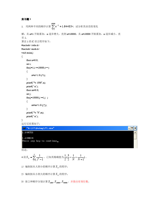
实习题11. 用两种不同的顺序计算644834.11000012≈∑=-n n,试分析其误差的变化解:从n=1开始累加,n 逐步增大,直到n=10000;从n=10000开始累加,n 逐步减小,直至1。
算法1的C 语言程序如下: #include<stdio.h> #include<math.h> void main() { float n=0.0; int i; for(i=1;i<=10000;i++) { n=n+1.0/(i*i); } printf("%-100f",n); printf("\n"); float m=0.0; int j; for(j=10000;j>=1;j--) { m=m+1.0/(j*j); } printf("%-7f",m); printf("\n"); }运行后结果如下:结论: 4.设∑=-=Nj N j S 2211,已知其精确值为)11123(21+--N N 。
1)编制按从大到小的顺序计算N S 的程序; 2)编制按从小到大的顺序计算N S 的程序;3)按2种顺序分别计算30000100001000,,S S S ,并指出有效位数。
解:1)从大到小的C语言算法如下:#include<stdio.h>#include<math.h>#include<iostream>using namespace std;void main(){float n=0.0;int i;int N;cout<<"Please input N"<<endl;cin>>N;for(i=N;i>1;i--){n=n+1.0/(i*i-1);N=N-1;}printf("%-100f",n);printf("\n");}执行后结果为:N=2时,运行结果为:N=3时,运行结果为:N=100时,运行结果为:N=4000时,运行结果为:2)从小到大的C语言算法如下:#include<stdio.h>#include<math.h>#include<iostream>using namespace std;void main(){float n=0.0;int i;int N;cout<<"Please input N"<<endl;cin>>N;for(i=2;i<=N;i++){n=n+1.0/(i*i-1);}printf("%-100f",n);printf("\n");}执行后结果为:N=2时,运行结果为:N=3时,运行结果为:N=100时,运行结果为:N=4000时,运行结果为:结论:通过比较可知:N 的值较小时两种算法的运算结果相差不大,但随着N 的逐渐增大,两种算法的运行结果相差越来越大。
计算方法实验报告习题2(浙大版)
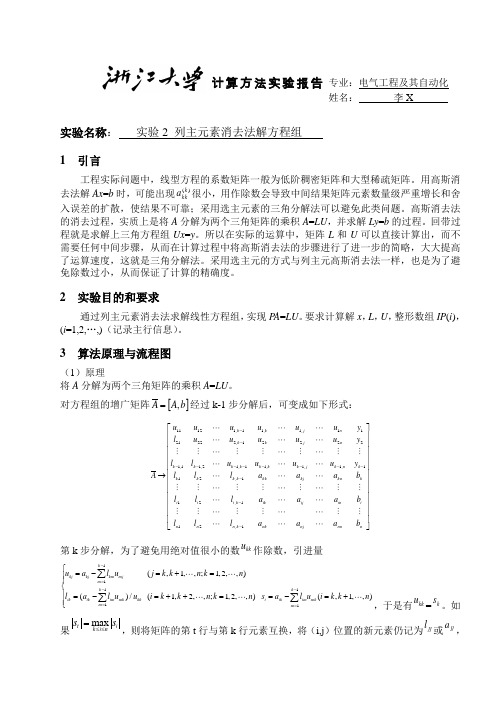
计算方法实验报告实验名称: 实验2 列主元素消去法解方程组 1 引言工程实际问题中,线型方程的系数矩阵一般为低阶稠密矩阵和大型稀疏矩阵。
用高斯消去法解Ax =b 时,可能出现)(k kk a 很小,用作除数会导致中间结果矩阵元素数量级严重增长和舍入误差的扩散,使结果不可靠;采用选主元素的三角分解法可以避免此类问题。
高斯消去法的消去过程,实质上是将A 分解为两个三角矩阵的乘积A =LU ,并求解Ly =b 的过程。
回带过程就是求解上三角方程组Ux =y 。
所以在实际的运算中,矩阵L 和U 可以直接计算出,而不需要任何中间步骤,从而在计算过程中将高斯消去法的步骤进行了进一步的简略,大大提高了运算速度,这就是三角分解法。
采用选主元的方式与列主元高斯消去法一样,也是为了避免除数过小,从而保证了计算的精确度。
2 实验目的和要求通过列主元素消去法求解线性方程组,实现P A =LU 。
要求计算解x ,L ,U ,整形数组IP (i ),(i =1,2,…,)(记录主行信息)。
3 算法原理与流程图(1)原理将A 分解为两个三角矩阵的乘积A =LU 。
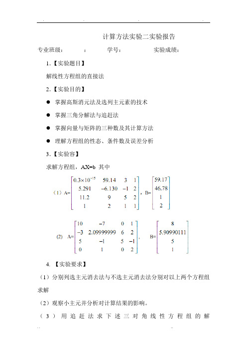
对方程组的增广矩阵[]b A A ,=经过k-1步分解后,可变成如下形式:⎥⎥⎥⎥⎥⎥⎥⎥⎥⎥⎥⎥⎦⎤⎢⎢⎢⎢⎢⎢⎢⎢⎢⎢⎢⎢⎣⎡→-------------n nnnjnkk n n n i in ij ik k i i i k kn kj kk k k k k k n k j k k k k k k k n j k k n j k k b a a a l l l b a a a l l l b a a a l l l y u u u u l l y u u u u u l y u u u u u u A1,211,211,211,1,1,11,12,11,122221,2222111,1,11,11211第k 步分解,为了避免用绝对值很小的数kku 作除数,引进量1111 (,1,,;1,2,,) ()/ (1,2,,;1,2,,)k kj kj km mj m k ik ik im mk kk m u a l u j k k n k n l a l u u i k k n k n -=-=⎧=-=+=⎪⎪⎨⎪=-=++=⎪⎩∑∑11(,1,,)k i ik im mkm s a l u i k k n -==-=+∑,于是有kk u =ks 。
计算方法-解线性方程组的直接法实验报告
cout<<endl;
for(k=i+1;k<m;k++)
{
l[k][i]=a[k][i]/a[i][i];
for(r=i;r<m+1;r++) /*化成三角阵*/
a[k][r]=a[k][r]-l[k][i]*a[i][r];
}
}
x[m-1]=a[m-1][m]/a[m-1][m-1];
{
int i,j;
float t,s1,s2;
float y[100];
for(i=1;i<=n;i++) /*第一次回代过程开始*/
{
s1=0;
for(j=1;j<i;j++)
{
t=-l[i][j];
s1=s1+t*y[j];
}
y[i]=(b[i]+s1)/l[i][i];
}
for(i=n;i>=1;i--) /*第二次回代过程开始*/
s2=s2+l[i][k]*u[k][r];
l[i][r]=(a[i][r]-s2)/u[r][r];
}
}
printf("array L:\n");/*输出矩阵L*/ for(i=1;i<=n;i++)
{
for(j=1;j<=n;j++)
printf("%7.3f ",l[i][j]);
printf("\n");
{
s2=0;
for(j=n;j>i;j--)
计算方法实验报告(附代码)
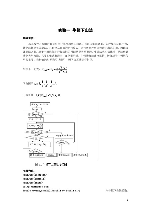
实验一 牛顿下山法实验说明:求非线性方程组的解是科学计算常遇到的问题,有很多实际背景.各种算法层出不穷,其中迭代是主流算法。
只有建立有效的迭代格式,迭代数列才可以收敛于所求的根。
因此设计算法之前,对于一般迭代进行收敛性的判断是至关重要的。
牛顿法也叫切线法,是迭代算法中典型方法,只要初值选取适当,在单根附近,牛顿法收敛速度很快,初值对于牛顿迭代 至关重要。
当初值选取不当可以采用牛顿下山算法进行纠正。
牛顿下山公式:)()(1k k k k x f x f x x '-=+λ下山因子 ,,,,322121211=λ下山条件|)(||)(|1k k x f x f <+实验代码:#include<iostream> #include<iomanip> #include<cmath>using namespace std;double newton_downhill(double x0,double x1); //牛顿下山法函数,返回下山成功后的修正初值double Y; //定义下山因子Y double k; //k为下山因子Y允许的最小值double dfun(double x){return 3*x*x-1;} //dfun()计算f(x)的导数值double fun1(double x){return x*x*x-x-1;} //fun1()计算f(x)的函数值double fun2(double x) {return x-fun1(x)/dfun(x);} //fun2()计算迭代值int N; //N记录迭代次数double e; //e表示要求的精度int main(){double x0,x1;cout<<"请输入初值x0:";cin>>x0;cout<<"请输入要求的精度:";cin>>e;N=1;if(dfun(x0)==0){cout<<"f'(x0)=0,无法进行牛顿迭代!"<<endl;}x1=fun2(x0);cout<<"x0"<<setw(18)<<"x1"<<setw(18)<<"e"<<setw(25)<<"f(x1)-f(x0)"<<endl;cout<<setiosflags(ios::fixed)<<setprecision(6)<<x0<<" "<<x1<<" "<<fabs(x1-x0)<<" "<<fabs(fun1(x1))-fabs(fun1(x0))<<endl;if(fabs(fun1(x1))>=fabs(fun1(x0))){ //初值不满足要求时,转入牛顿下山法x1=newton_downhill(x0,x1);} //牛顿下山法结束后,转入牛顿迭代法进行计算while(fabs(x1-x0)>=e){ //当精度不满足要求时N=N+1;x0=x1;if(dfun(x0)==0){cout<<"迭代途中f'(x0)=0,无法进行牛顿迭代!"<<endl;} x1=fun2(x0);cout<<setiosflags(ios::fixed)<<setprecision(6)<<x0<<" "<<x1<<" "<<fabs(x1-x0)<<endl;}cout<<"迭代值为:"<<setiosflags(ios::fixed)<<setprecision(6)<<x1<<'\n';cout<<"迭代次数为:"<<N<<endl;return 0;}double newton_downhill(double x0,double x1){Y=1;cout<<"转入牛顿下山法,请输入下山因子允许的最小值:";cin>>k;while(fabs(fun1(x1))>=fabs(fun1(x0))){if(Y>k){Y=Y/2;}else {cout<<"下山失败!";exit(0);}x1=x0-Y*fun1(x0)/dfun(x0);}//下山成功则cout<<"下山成功!Y="<<Y<<",转入牛顿迭代法计算!"<<endl;return x1;}实验结果:图4.1G-S 迭代算法流程图实验二 高斯-塞德尔迭代法实验说明:线性方程组大致分迭代法和直接法。
计算方法实验报告
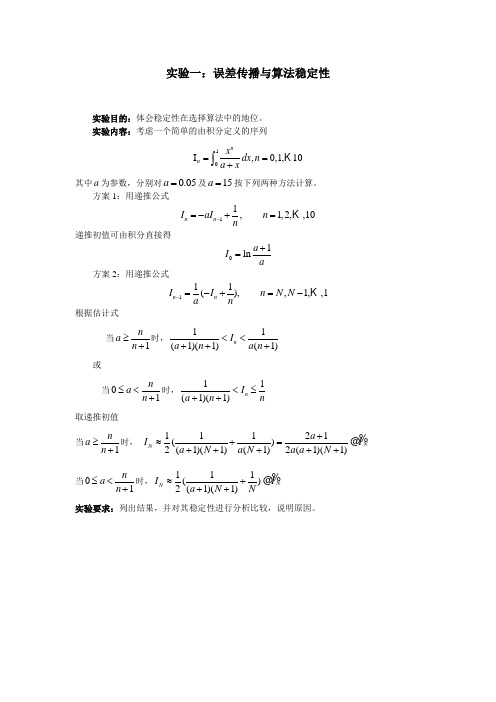
实验一:误差传播与算法稳定性实验目的:体会稳定性在选择算法中的地位。
实验内容:考虑一个简单的由积分定义的序列10I ,0,1,10nn x dx n a x==+⎰其中a 为参数,分别对0.05a =及15a =按下列两种方法计算。
方案1:用递推公式11,1,2,,10n n I aI n n-=-+= 递推初值可由积分直接得01lna I a+= 方案2:用递推公式111(),,1,,1n n I I n N N a n-=-+=-根据估计式当1n a n ≥+时,11(1)(1)(1)n I a n a n <<+++或当01n a n ≤<+时,11(1)(1)n I a n n<≤++ 取递推初值 当1n a n ≥+时, 11121()2(1)(1)(1)2(1)(1)N N a I I a N a N a a N +≈+=+++++ 当01n a n ≤<+时,111()2(1)(1)N N I I a N N≈+++ 实验要求:列出结果,并对其稳定性进行分析比较,说明原因。
实验二:非线性方程数值解法实验目的:探讨不同方法的计算效果和各自特点 实验内容:应用算法(1)牛顿法;(2)割线法 实验要求:(1)用上述各种方法,分别计算下面的两个例子。
在达到精度相同的前提下,比较其迭代次数。
(I )31080x x +-=,取00x =;(II) 2281(0.1)sin 1.060x x x -+++=,取00x =;(2) 取其它的初值0x ,结果如何?反复选取不同的初值,比较其结果; (3) 总结归纳你的实验结果,试说明各种方法的特点。
实验三:选主元高斯消去法----主元的选取与算法的稳定性问题提出:Gauss 消去法是我们在线性代数中已经熟悉的。
但由于计算机的数值运算是在一个有限的浮点数集合上进行的,如何才能确保Gauss 消去法作为数值算法的稳定性呢?Gauss 消去法从理论算法到数值算法,其关键是主元的选择。
计算方法实验报告_列主元高斯消去法

row_first=A[i][i]; for(int j=0;j<n+1;j++)
计算方法实验报告
{ A[i][j]=A[i][j]/row_first;
} }
for(int k=n-1;k>0;k--) {
for(int i=0;i<N;i++) {
for(int j=0;j<N;j++) {
A_B[i][j]=A[i][j]; } A_B[i][N]=B[i][0]; } return A_B; }
3
//输出矩阵 A 的 row x col 个元素 void Show_Matrix(double **A,int row,int col) {
for(int i=0;i<N;i++)
{
int row=Choose_Colum_Main_Element(N,A_B,i);
if(Main_Element<=e) goto A_0;
Exchange(A_B,N+1,row,i);
Elimination(N,A_B,i);
cout<<"选取列主元后第"<<i+1<<"次消元:"<<endl;
double factor; for(int i=start+1;i<n;i++) {
factor=A[i][start]/A[start][start]; for(int j=start;j<n+1;j++) {
计算方法实验报告01
y13=polyval(p3,t)
y14=polyval(p4,t)
r1=sum((y1-y11).^2)
r2=sum((y2-y12).^2)
r3=sum((y1-y13).^2)
r4=sum((y2-y14).^2)
plot(t,y11,'r',t,y12,'b')
plot(t,y13,'r',t,y14,'b')
4. 程序运行结果及分析(输出计算结果,结果分析)
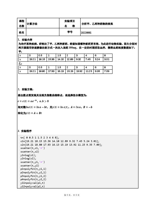
分别画出t与浓度c的散点图(上图代表甲,下图代表乙):
分别画出t与浓度的对数y(t)=ln c(t)的散点图(上图代表甲,下图代表乙)
进行一次多项式拟合得:
y1(t)=−0.2319t+2.9795
y2(t)=−0.1278t+2.9829
进行二次多项式拟合得:
y1(t)=−0.2322t+2.9798
y2(t)=−0.1278t+2.9830
进行一次多项式拟合得到拟合曲线如图(下方代表甲,上方代表乙):
进行二次多项式拟合得到拟合曲线如图(下方代表甲,上方代表乙):
对数值结果进行分析:
进行一次多项式拟合误差平方和分别为:
r1=0.0137
r2=0.0063
进行一次多项式拟合误差平方和分别为:
r1=0.0137
r2=0.0063
经分析:
本次实验一次多项式拟合和二次多项式拟合相差不大;。
《计算方法》实验报告
《计算方法》实验报告一、实验目的本次《计算方法》实验的主要目的是通过实际操作和编程实现,深入理解和掌握常见的计算方法在解决数学问题中的应用。
通过实验,提高我们运用数学知识和计算机技术解决实际问题的能力,培养我们的逻辑思维和创新能力。
二、实验环境本次实验使用的编程语言为 Python,使用的开发工具为 PyCharm。
实验运行的操作系统为 Windows 10。
三、实验内容与步骤1、线性方程组的求解实验内容:使用高斯消元法和LU分解法求解线性方程组。
实验步骤:首先,定义线性方程组的系数矩阵和常数向量。
对于高斯消元法,通过逐步消元将系数矩阵化为上三角矩阵,然后回代求解。
对于 LU 分解法,将系数矩阵分解为下三角矩阵 L 和上三角矩阵 U,然后通过向前和向后代换求解。
2、插值与拟合实验内容:使用拉格朗日插值法、牛顿插值法进行插值计算,并使用最小二乘法进行曲线拟合。
实验步骤:对于拉格朗日插值法和牛顿插值法,根据给定的节点数据计算插值多项式。
对于最小二乘法,根据给定的数据点和拟合函数形式,计算拟合参数。
3、数值积分实验内容:使用矩形法、梯形法和辛普森法计算定积分。
实验步骤:定义被积函数和积分区间。
对于矩形法,将积分区间等分为若干小区间,每个小区间用矩形面积近似积分值。
梯形法通过构建梯形来近似积分值。
辛普森法利用抛物线来近似积分值。
4、常微分方程的数值解法实验内容:使用欧拉法和改进的欧拉法求解常微分方程。
实验步骤:给定常微分方程和初始条件。
按照欧拉法和改进的欧拉法的公式进行迭代计算,得到数值解。
四、实验结果与分析1、线性方程组的求解高斯消元法和 LU 分解法都能成功求解线性方程组,但在计算效率和数值稳定性上可能存在差异。
对于规模较大的线性方程组,LU 分解法通常更具优势。
实验中通过对比不同方法求解相同线性方程组的结果,验证了算法的正确性。
2、插值与拟合拉格朗日插值法和牛顿插值法在给定节点处能够准确插值,但对于节点之外的区域,可能会出现较大偏差。
计算方法 实验报告 拉格朗日 龙贝格 龙格库塔

主界面:
/*lagrange.c*/
float real_value(float x) /*由被插值函数计算真实值*/
c=getchar();
if(c=='N'||c=='n') break;
}
}
/*romberg.c*/
double function(double x) /*被积函数*/
{
return 4.0/(1+(x)*(x));
}
double t(double a,double b,int m) /*计算T1*/
实验二(龙贝格公式)
§公式
§算法描述
§流程图
§运行结果
§结果分析:Romberg积分法是在积分步长逐步折半的过程中,用低精度求积公式的组合得到更高精度求积公式的一种方法,它算法简单,且收敛加速效果极其显著。
实验三(四阶龙格库塔)
§公式
k1=h*f(xn,yn);
k2=h*f(xn+h/2,yn+k1/2);
T1=t(a,b,0);
T2=T1/2.0+t(a,b,1);
S1=(4*T2-T1)/3.0;
T1=T2;
T2=T1/2.0+t(a,b,2);
S2=(4*T2-T1)/3.0;
C1=(16*S2-S1)/15.0;
T1=T2;
T2=T1/2.0+t(a,b,3);
S1=S2;
S2=(4*T2-T1)/3.0;
计算方法实验二
《计算方法》实验报告实验二插值法二级学院:计算机学院专业:计算机科学与技术指导教师:爨莹班级学号:姓名:实验二插值法1、实验目的:1、掌握直接利用拉格郎日插值多项式计算函数在已知点的函数值;观察拉格郎日插值的龙格现象。
2、了解Hermite插值法、三次样条插值法原理,结合计算公式,确定函数值。
2、实验要求:1、认真分析题目的条件和要求,复习相关的理论知识,选择适当的解决方案和算法;2、编写上机实验程序,作好上机前的准备工作;3、上机调试程序,并试算各种方案,记录计算的结果(包括必要的中间结果);4、分析和解释计算结果;5、按照要求书写实验报告;3、实验内容:1、用拉格郎日插值公式确定函数值;对函数f(x)进行拉格郎日插值,并对f(x)与插值多项式的曲线作比较。
2、已知函数表:(0.56160,0.82741)、(0.56280,0.82659)、(0.56401,0.82577)、(0.56521,0.82495)用三次拉格朗日插值多项式求x=0.5635时函数近似值。
3、P129,(12)4、题目:插值法5、原理:拉格朗日插值法是以法国十八世纪数学家约瑟夫·路易斯·拉格朗日命名的一种多项式插值方法。
许多实际问题中都用函数来表示某种内在联系或规律,而不少函数都只能通过实验和观测来了解。
如对实践中的某个物理量进行观测,在若干个不同的地方得到相应的观测值,拉格朗日插值法可以找到一个多项式,其恰好在各个观测的点取到观测到的值。
这样的多项式称为拉格朗日(插值)多项式。
数学上来说,拉格朗日插值法可以给出一个恰好穿过二维平面上若干个已知点的多项式函数。
6、设计思想:通过拉格朗日插值法找到拉格朗日多项式,计算某个x对应的y值。
7、对应程序://Lagrange.cpp#include <stdio.h>#include <conio.h>#define N 4int checkvalid(double x[], int n);void printLag (double x[], double y[], double varx, int n);double Lagrange(double x[], double y[], double varx, int n);void main (){double x[N+1] = {0.56160, 0.56280, 0.56401, 0.56521};double y[N+1] = {0.82741, 0.82659, 0.82577, 0.82459};double varx = 0.5635;if (checkvalid(x, N) == 1){printf("\n\n插值结果: P(%f)=%f\n", varx, Lagrange(x, y, varx, N));}else{printf("结点必须互异");}getch();}int checkvalid (double x[], int n){int i,j;for (i = 0; i < n; i++){for (j = i + 1; j < n+1; j++){if (x[i] == x[j])//若出现两个相同的结点,返回-1{return -1;}}}return 1;}double Lagrange (double x[], double y[], double varx, int n){double fenmu;double fenzi;double result = 0;int i,j;printf("Ln(x) =\n");for (i = 0; i < n+1; i++){fenmu = 1;for (j = 0; j < n+1; j++){if (i != j){fenmu = fenmu * (x[i] - x[j]);}}printf("\t%f", y[i] / fenmu);fenzi = 1;for (j = 0; j < n+1; j++){if (i != j){printf("*(x-%f)", x[j]);fenzi = fenzi * (varx - x[j]);}}if (i != n){printf("+\n");}result += y[i] / fenmu * fenzi;}return result;}8、实验结果:9、实验体会:拉格朗日插值法能很好的解决生产和科研中的一些问题,计算机编程的实现有利于其更好的应用。
计算方法数值实验报告
计算方法数值实验报告(一)班级:0902 学生:苗卓芳 倪慧强 岳婧实验名称: 解线性方程组的列主元素高斯消去法和LU 分解法实验目的: 通过数值实验,从中体会解线性方程组选主元的必要性和LU 分解法的优点,以及方程组系数矩阵和右端向量的微小变化对解向量的影响。
实验内容:解下列两个线性方程组(1) ⎪⎪⎪⎭⎫ ⎝⎛=⎪⎪⎪⎭⎫ ⎝⎛⎪⎪⎪⎭⎫ ⎝⎛--11134.981.4987.023.116.427.199.103.601.3321x x x (2) ⎪⎪⎪⎪⎪⎭⎫ ⎝⎛=⎪⎪⎪⎪⎪⎭⎫ ⎝⎛⎪⎪⎪⎪⎪⎭⎫ ⎝⎛----15900001.582012151526099999.23107104321x x x x 解:(1) 用熟悉的算法语言编写程序用列主元高斯消去法和LU 分解求解上述两个方程组,输出Ax=b 中矩阵A 及向量b, A=LU 分解的L 及U ,detA 及解向量。
①先求解第一个线性方程组⎪⎪⎪⎭⎫ ⎝⎛=⎪⎪⎪⎭⎫ ⎝⎛⎪⎪⎪⎭⎫ ⎝⎛--11134.981.4987.023.116.427.199.103.601.3321x x x在命令窗口中运行A=[3.01,6.03,1.99;1.27,4.16,-1.23;0.987,-4.81,9.34] 可得A =3.0100 6.0300 1.99001.2700 4.1600 -1.23000.9870 -4.8100 9.3400b=[1,1,1]可得b =1 1 1H =det(A)可得 H =-0.0305列主元高斯消去法:在命令窗口中运行function x=Gauss_pivot(A,b)、A=[3.01,6.03,1.99;1.27,4.16,-1.23;0.987,-4.81,9.34];b=[1,1,1];n=length(b);x=zeros(n,1);c=zeros(1,n);dl=0;for i=1:n-1max=abs(A(i,i));m=i;for j=i+1:nif max<abs(A(j,i))max=abs(A(j,i));m=j;endendif(m~=i)for k=i:nc(k)=A(i,k);A(i,k)=A(m,k);A(m,k)=c(k);enddl=b(i);b(i)=b(m);b(m)=dl;endfor k=i+1:nfor j=i+1:nA(k,j)=A(k,j)-A(i,j)*A(k,i)/A(i,i);endb(k)=b(k)-b(i)*A(k,i)/A(i,i);A(k,i)=0;endendx(n)=b(n)/A(n,n);for i=n-1:-1:1sum=0;for j=i+1:nsum =sum+A(i,j)*x(j);endx(i)=(b(i)-sum)/A(i,i);end经程序可得实验结果ans =1.0e+003 *1.5926-0.6319-0.4936LU分解法:在命令窗口中运行function x=lu_decompose(A,b)A=[3.01,6.03,1.99;1.27,4.16,-1.23;0.987,-4.81,9.34];b=[1,1,1];L=eye(n);U=zeros(n,n);x=zeros(n,1);c=zeros(1,n);for i=1:nU(1,i)=A(1,i);if i==1;L(i,1)=1;elseL(i,1)=A(i,1)/U(1,1);endendfor i=2:nfor j=i:nsum=0;for k=1:i-1sum =sum+L(i,k)*U(k,j);endU(i,j)=A(i,j)-sum;Ifj~=nsum=0;for k=1:i-1sum=sum+L(j+1,k)*U(k,i);endL(j+1,i)=(A(j+1,i)-sum)/U(I,i);endendendy(1)=b(1);for k=2:nsum=0;forj=1:k-1sum=sum+L(k,j)*y (j);endy(k)=b(k)-sum;endx(n)=y(n)/U(n,n);260页最后一行c(k)=A(i,k);A(i,k)=A(m,k);A(m,k)=c(k);enddl=b(i);b(i)=b(m);b(m)=dl;endfor k=i+1:nfor j=i+1:nA(k,j)=A(k,j)-A(i,j)*A(k,i)/A(i,i);endb(k)=b(k)-b(i)*A(k,i)/A(i,i);A(k,i)=0;endendx(n)=b(n)/A(n,n);for i=n-1:-1:1sum=0;for j=i+1:nsum =sum+A(i,j)*x(j);endx(i)=(b(i)-sum)/A(i,i);end经程序可得结果ans =1.0e+003 *1.5926-0.6319-0.4936②再求解第二个线性方程组⎪⎪⎪⎪⎪⎭⎫ ⎝⎛=⎪⎪⎪⎪⎪⎭⎫ ⎝⎛⎪⎪⎪⎪⎪⎭⎫ ⎝⎛----15900001.582012151526099999.23107104321x x x x 即A=[10,-7,0,1;-3,2.099999,6,2;5,-1,5,-1;2,1,0,2];b=[8,5.900001,5,1];重复上述步骤可的结果为ans =0.0000-1.00001.00001.0000(2)将方程组(1)中系数3.01改为3.00,0.987改为0.990,用列主元高斯消去法求解变换后的方程组,输出列主元行交换次序,解向量x 及detA ,并与(1)中结果比较。
华南理工大学《计算方法》实验报告

华南理工大学《计算方法》实验报告华南理工大学《计算方法》实验报告学院计算机科学与工程专业计算机科学与技术(全英创新班)学生姓名 -------学生学号 ------------指导教师布社辉课程编号 145022课程学分 3 分起始日期 2015年5月28日实验题目一Solution of Nonlinear Equations--Bracketing method and Newton-Raphson method姓名:xxxxxx学号:xxxxxxxxxxxx时间:2015年5月28日【题目】1.Find an approximation (accurate to 10 decimal places) for the interest rate I thatwill yield a total annuity value of $500,000 if 240 monthly payments of $300 are made.2.Consider a spherical ball of radius r = 15 cm that is constructed from a variety ofwhite oak that has a density of ρ = 0.710. How much of the ball (accurate to eight decimal places) will be submerged when it is placed in water?3.To approximate the fixed points (if any) of each function. Answers should beaccurate to 12 decimal places. Produce a graph of each function and the line y = x that clearly shows any fixed points.(a) g(x) = x5 − 3x3 − 2x2 + 2(b) g(x) = cos(sin(x))【实验分析】1.Assume that the value of the k-th month is , the value next month is, whereSo the total annuity value after 240 months is :To find the rate I that satisfied A=5000000, we can find the solution to the equationThe Bisection method can be used to find the solution of .2.The mass of water displaced when a sphere is submerged to a depth d is:The mass of the ball isAppl ying Archimedes’ law, , produce the following equations:So g(d)=, and Bisection method can be used to find the root.3.In this problem, the target is to find the fixed point by fixed point iteration. So wecan use fixed point iteration method to solve the problem.(a),so ,Plot the function g(x) and y=x, it can be seen that there are three fixed point, where ,It can be solved that:for,for,for,So, ,,, they are all repelling fixed point, fixed point iteration method cannot converge to them.(b). From the graph below we know that the fixed point liesbetween 0.5 and 1. Where . So the fixed point is attractive fixed point. I initially guess that p=0.75, and apply fixed point iteration method to find the solution.【实验过程和程序】1.The value of g(I) will change significantly but little change of I, so that it’sunwise to plot the figure about I and g(I). Instead, the interest will be bound by [0,1] by common sense. So I set the left end point of Bisection method to 0, right end point to 1. The precision is set to 1e-10.Code for g(I) is :Code for applying Bisection method is :2.The since the density of the ball is smaller than water, so depth submerged shouldnot be larger than 2r, and not less than 0. So I set the left end point of Bisection method to 0 and right to 2r.Code for g(d) is :Code for applying Bisection method is :3.(a)Code for function g:Code for applying fixed point iteration:Code for plot the graph:(b)Code of this problem is similar to the previous one, so it’s not illustrated here.【实验结果】1.Result for the program is :So the annual interest rate is 31.78710938%2.X-axis is the depth and Y-axis is for g(d). Blue line is the function value versusdepth. Red line is y=0. It can be seen from the graph that the solution is about 19.And by using Bisection method, the solution depth=19.306641cm is found, with8 significance bit.3.(a) No fixed point can be found. By solving this equation, we can find that x=2 isone of the solution. If we set the initial point to 2.00000000001 or 1.9999999, the result is the same:. If we set initial point to 2, the point can be found:. This is consistent with the conclusion discussed in the previous part.(b)The fixed point p=0.768169156736 is found:实验题目二Solution of Linear Systems--Gaussian elimination and pivoting姓名:xxxxxx学号:xxxxxxxxxxxx时间:2015年5月28日【题目】Find the sixth-degree polynomial y = a1 + a2x + a3x^2 + a4x^3 + a5x^4 + a6x^5 + a7x^6 that passes through (0, 1), (1, 3), (2, 2), (3, 1), (4, 3), (5, 2), and (6, 1). Use the plot command to plot the polynomial and the given points on the same graph. Explain any discrepancies in your graph.【实验分析】To find the coefficient of each term, we can substitute all the given point to the equations and construct an argument matrix AX=B. Then perform triangular factorization and solve the upper-triangular and lower triangular matrix by back substitution method.Since det(A) = 2.4883e+07 ≠ 0,there exist a unique solution for AX=B.【实验过程和程序】Code for construct coefficient matrix A:Code for construct matrix B:Solve X by triangular factorization and back substitution method:【实验结果】The result for coefficient matrix:The graph of the polynomial is shown below. Blue lines denotes the graph for the polynomial and red points are the sample points. This polynomial fits the points well.Iterat ion of Linear System’s solution--Seidel iteration姓名:xxxxxx学号:xxxxxxxxxxxx时间:2015年5月28日【题目】(a)Start with P0 = 0 and use Jacobi iteration to find Pk for k = 1, 2, 3. Will Jacobi iteration converge to the solution?(b) Start with P0 = 0 and use Gauss-Seidel iteration to find Pk for k = 1, 2, 3. Will Gauss-Seidel iteration converge to the solution?【实验分析】In this problem we only need to construct the coefficient matrix and matrix B and then apply the Jacobi Iteration method and Gauss-Seidel Iteration method to find the solution. SinceA satisfy strictly diagonally dominant, so the iteration steps will converge.【实验过程和程序】【实验结果】Points in first three iteration is shown below. Both this two method will converge.Interpolation--Spline interpolation姓名:xxxxxx学号:xxxxxxxxxxxx时间:2015年5月28日【题目】The measured temperatures during a 5-hour period in a suburb of Los Angeles on November 8 are given in the following table.(a)To construct a Lagrange interpolatory polynomial for the data in the table.(b)To estimate the average temperature during the given5-hour period.(c)Graph the data in the table and the polynomial frompart (a) on the same coordinate system. Discuss thepossible error that can result from using thepolynomial in part (a) to estimate the averagetemperature.【实验分析】(a)X=[1,2,3,4,5,6] Y=[66,66,65,64,63,63], the target is to construct a Lagrangeinterpolatory polynomial for X and Y. We can apply the Lagrange approximation method to solve it.(b)After we get the interpolatory polynomial, we can use a great amount of samplepoints and estimate the function value of them and take the mean.(c)Error contain in Lagrange interpolatory polynomial of 5-degree is:, where Error on the average temperature equals to the mean of , which is:Error ====240.06【实验过程和程序】(a)Construct X and Y, and solve it by Lagrange approximation:(b)After we get the polynomial function, we calculate function value on a set ofsample points and get their mean as the average temperature.(c)plot X_new and Y_new in part(b) is equivalent to plot P N(x). And error bound canonly be obtain by analyzing since f(x) is unknown.【实验结果】(a) We can get the result:Which means that:(b)By taking the mean, the average temperature is 64.5℉:(c)The graph for polynomial and the sample points is shown below. Error bound forthe average temperature is 240.06.实验题目五Curve Fitting--Least mean square error姓名:xxxxxx学号:xxxxxxxxxxxx时间:2015年5月28日【题目】1.The temperature cycle in a suburb of Los Angeles on November 8 is given in theaccompanying table. There are 24 data points.(a)Follow the procedure outlined in Example5.5 (use the fmins command) to find theleast-squares curve of the form f (x) = Acos(Bx)+C sin(Dx)+ E for the given set ofdata.(b)Determine E2( f ).(c)Plot the data and the least-squares curvefrom part (a) on the same coordinatesystem.【实验分析】(a)In this problem. The hour 1~midnight p.m. can be map to 1~12, 1~noon a.m. canbe map to 13~24. So hour and temperature can be used to fit the curve. To get the curve with minimum error, which is define as:The best A, B, C, D, E can be found when:(b)is defined as:In our case,【实验过程和程序】(a) The function of the error is:Using command, A B C D E can be solved. (b) By the function solved by part(a), we can calculate for each sample pointand then calculate :(c) Code to plot the line:【实验结果】(a)The result for parameter A B C D E is:So the least-squares curve is :(b)Error for f(x) is:(c)Graph for least-squares curve and sample points is:Notice that the result of function fminesarch is sensitive about the input seeds.Firstly the seed is [1 1 1 1 1], and get the result [0.1055 -2.1100 0.9490 -4.869861.0712]. In second step, seed is [0.1 2 1 -5 61] and result is [0.0932 2.11141.175 -5.127 61.0424]. By 4 iterations, I find a good fit of the data and get the seed[1 0.1 1 1 60].Numerical Integration--Automatically select the integration step of the trapezoidal method姓名:xxxxxx学号:xxxxxxxxxxxx时间:2015年5月28日【题目】(i) Approximate each integral using the compositetrapezoidal rule with M = 10.(ii) Approximate each integral using the compositeSimpson rule with M = 5.【实验分析】The formula of each function is given in this problem, so we just need to use composite trapezoidal rule and composite Simpson rule to solve them.【实验过程和程序】Function of the six equations:Code for calculation:【实验结果】Solution of Differential Equations--Euler’s Method and Heun’s Method姓名:xxxxxx学号:xxxxxxxxxxxx时间:2015年5月28日【题目】(Supplement) A skydiver jumps from a plane, and up to the moment he opens theparachute the air resistance is proportional to (v represents velocity). Assume that the time interval is [0,6] and hat the differential equation for the downward direction isover [0,6] with v(0)=0Use Euler’s method with h=0.05 and estimate v(6).【实验分析】The function of , where left end point is 0 and right is 6, with initial point v(0)=0. So we can apply Euler’s method directory to solve the problem.【实验过程和程序】Function of :Code of applying Euler’s method:【实验结果】….,so v(6)=10.0726.。
计算方法实验报告

Matelab 实习三一.题目1.对于给函数f(x)=1/(1+25x^2)在区间[-1,1]上取Xi=-1+0.2i (i=0,1,…10),试求三次曲线拟合,试画出拟合曲线并打印方程,与第2章计算实习题2的结果比较。
试求3次、4次多项式的曲线拟合,再根据数据曲线形状,求一个另外函数的拟合曲线,用图示数据曲线及相应的三种拟合曲线。
3.使用快速傅里叶变换确定函数)cos()(2x x x f =在[-pi,pi]上的16次三角插值多项式。
二.实验理论1.,由此求出格拉姆矩阵G ,可写成矩阵形式:Ga=d 。
实验中,只要求出矩阵G 和向量d ,即可由Ga=d 得出ai(i=0,1,2 …n),进而可求出S(x)=∑ai*x^i.2.,可写成矩阵形式: Ga=d 。
实验中,只要求出矩阵G 和向量d ,即可由Ga=d 得出ai(i=0,1,2 …n)进而可求出S(x)=∑ai*x^i.3.FFT 计算公式如下:其中q=1,2,…p,k=0,1,…2^(p -q)-1,j=0,1,…2^(q -1)-1。
经过不断的二分迭代,可得到Ap(j).即Ck ,而ak=real(Ck),bk=image(Ck),∑-=+++=11)sin cos (21n k n k k a ky b ky a S三.实验程序1.function [ output_args ] = triRunge(m)n=m+1;x=zeros(1,11);y=zeros(1,11);x(1)=-1;for i =1:10x(i+1)=-1+0.2*i;end ```·,1,0,]),(==∑k d a k j j k ϕϕ ```·,1,0,]),(==∑k d a k j j k ϕϕ ```·,1,0,]),(==∑k d a k j j k ϕϕ ```·,1,0,]),(==∑k d a k j j k ϕϕ []12111111-q 11111)22(-)2()22(A )22()2()2(A -----------+++=++++++=+q k p q q q q q q p q q q q q q w j k A j k A j k j k A j k A j kfor i=1:11y(i)=1/(1+25*x(i)^2);endd=zeros(n,n); f=zeros(1,n); for i=1:nfor j=1:nfor k=1:11d(i,j)=d(i,j)+x(k)^(i+j-2);endendendfor i=1:nfor k=1:11f(i)=f(i)+x(k)^(i-1)*y(k);endenda=f/d; syms x;g=a(n)*x+a(n-1);for i=1:n-2g=g*x+a(n-2-i+1);endvpa(g);g=collect(g);g=vpa(g,3); ezplot(g,[-1,1]);gtext('拟合曲线');k=char(g);hold onezplot('1/(1+25*x^2)',[-1,1]);gtext('龙格函数1/(1+25x^2)');gtext(k)title('三次曲线拟合');end注:蓝色为3次拟合曲线,红色为龙格函数曲线可以看出:三次拟合曲线与龙格函数基本不重合,拟合效果差。
- 1、下载文档前请自行甄别文档内容的完整性,平台不提供额外的编辑、内容补充、找答案等附加服务。
- 2、"仅部分预览"的文档,不可在线预览部分如存在完整性等问题,可反馈申请退款(可完整预览的文档不适用该条件!)。
- 3、如文档侵犯您的权益,请联系客服反馈,我们会尽快为您处理(人工客服工作时间:9:00-18:30)。
《计算方法》实验报告 学号
姓名 班级
实验项目名称
计算方法实验 一、实验名称 实验一 插值与拟合
二、实验目的:
(1)明确插值多项式和分段插值多项式各自的优缺点;
(2)编程实现拉格朗日插值算法,分析实验结果体会高次插值产生的龙格现象;
(3)运用牛顿插值方法解决数学问题。
三、实验内容及要求
(1) 对于55,11)(2≤≤-+=x x
x f 要求选取11个等距插值节点,分别采用拉格朗日插值和分段线性插值,计算x 为0.5, 4.5处的函数值并将结果与精确值进行比较。
输入:区间长度,n(即n+1个节点),预测点
输出:预测点的近似函数值,精确值,及误差
(2)已知,,,392411===用牛顿插值公式求5的近似值。
输入:数据点集,预测点。
输出:预测点的近似函数值
四、实验原理及算法描述
算法基本原理:
(1)拉格朗日插值法
(2)牛顿插值法
算法流程
五、程序代码及实验结果
(1)输出:
A.拉格朗日插值法
B.分段线性插值
X y(精确) y(拉格朗日) y(分段线性) 误差(拉) 误差(分)
0.500000 0.800000 0.843407 0.750000 -0.054259 0.050000
4.500000 0.047059 1.578720 0.0486425 -32.547674 -0.033649
(2)输出:
X y(精确) y(牛顿插值) 误差(牛顿插值)
5.00000 2.236068 2.266670 -0.013686
源码:
(1)A.拉格朗日插值法
#include<iostream>
#include<string>
#include<vector>
using namespace std;
double Lagrange(int N,vector<double>&X,vector<double>&Y,double x); int main(){
double p,b,c;
char a='n';
do{
cout<<"请输入差值次数n的值:"<<endl;
int N;
cin>>N;
vector<double>X(N,0);
vector<double>Y(N,0);
cout<<"请输入区间长度(a,b):"<<endl;
cin>>p;
cin>>b;
c=b-p;
c=c/(N-1);
for(int i=0;i<N;i++){
X[i]=p;
Y[i]=1/(1+p*p);
p=p+c;
}
cout<<"请输入要求值x的值:"<<endl;
double x;
cin>>x;。