线性系统理论-最小二乘法
2011第5章线性参数的最小二乘法处理

二、正规方程
线性参数的最小二乘法处理程序可归结为: 首先根据具体问题列出误差方程式; 再按最小二乘法原理,利用求极值的方法将误差 方程转化为正规方程; 然后求解正规方程,得到待求的估计量; 最后给出精度估计。
对于非线性参数,可先将其线性化,然后按上 述线性参数的最小二乘法处理程序去处理。
二、正规方程
xt
V L AXˆ
则等精度测量时线性参数的残余误差方程为
v1
v1
v2
...
vn
v... 2
最小
vn
一、最小二乘法原理
V TV 最小 ( L AXˆ )T ( L AXˆ ) 最小
线性参数的不等精度测量还可以转化为等 精度的形式,从而可以利用等精度测量时测量 数据的最小二乘法处理的全部结果。
yn fn ( x1 , x2 , ..., xt )
一、最小二乘法原理
v1 l1 y1 v2 l2 y2
vn ln yn v1 l1 f1( x1 , x2 , ..., xt ) v2 l2 f2 ( x1 , x2 , ..., xt )
vn ln fn ( x1 , x2 , ..., xt )
ln
x1
Xˆ
...x2
xt
和
n×t
阶矩阵
A
a11
a21
a12 a22
... a1t
...
a2t
an1
an2
...
ant
最小二乘法线性详细说明

4
最小二乘法产生的历史
最小二乘法最早称为回归分析法。由著名的英 国生物学家、统计学家道尔顿(F.Gallton)— —达尔文的表弟所创。 早年,道尔顿致力于化学和遗传学领域的研究。 他研究父亲们的身高与儿子们的身高之间的关 系时,建立了回归分析法。
5
父亲的身高与儿子的身高之间关系的研究
1889年F.Gallton和他的朋友K.Pearson收集了 上千个家庭的身高、臂长和腿长的记录 企图寻找出儿子们身高与父亲们身高之间关系 的具体表现形式 下图是根据1078个家庭的调查所作的散点图 (略图)
vi = ∆yi = [ yi − (a + bxi )]
②
12
我们的目的是根据数据点确定回归常数a和b, 并且希望确定的a和b能使数据点尽量靠近直线 能使v尽量的小。由于偏差v大小不一,有正有 负,所以实际上只能希望总的偏差(∑ vi)最小。
2
所谓最小二乘法就是这样一个法则,按照这个 法则,最好地拟合于各数据点的最佳曲线应使 各数据点与曲线偏差的平方和为最小。
解方程,得:
sxy b=
⑥
sxx a = y − bx
⑦
16
公式⑥⑦式中:
sxy
xx
(∑ x ∑ y ) = ∑xy −
i i i i 2 i
2
(∑ x ) s = ∑x − x = ∑x n
i i
n
n
从④不难求出对a, b的二阶偏导数为: a, b
∂ ∑ vi 2 = 2n 2 ∂a ∂ ∑ vi 2 = 2∑ xi 2 2 ∂b ∂ ∑ vi 2 = 2∑ xi ∂a∂b
2
已经确定, 一 是物理量y与x间的函数关系已经确定 已经确定 只有其中的常数未定(及具体形式未定) 时,根据数据点拟合出各常数的最佳值。 未知时,从 二 是在物理量y与x间函数关系未知时 未知时 函数点拟合出y与x函数关系的经验公式以 及求出各个常数的最佳值。
第5章线性参数的最小二乘法处理

最小 1
p1 : p 2 : : p n
有
2 2
x1
2
2
:
n
1
x2
2
::
xn 2
( 55)
p1v1 p 2 v 2 p n v n
pi vi2
i 1
最小
对于等精度测量,有 1 1 n 即
p1 p 2 p n
2 2 n 12 2 2 2 2 最小 1 2 n
当然,由前述给出的结果只是估计量,它们以 最大的可能性接近真值而并非真值,因此上述条件 应以残差的形式表示,即用残差代替绝对误差:
2 v1 2
1 2 n 引入权的符号p,由下面的关系
2 2
2 v2
1
2 vn
2 i
0
2 2 2
0
为测量数据li的权; 为单位权方差;
0 0 2 2 n
i2为测量数据li的方差。
线性参数的不等精度测量可以转化为等精度的 形式(单位权化),从而可以利用等精度测量时 测量数据的最小二乘法处理的全部结果。为此, 应将误差方程化为等权的形式。若不等精度测量 数据li 的权为pi ,将不等精度测量的误差方程式 (5-9)两端同乘以相应权的平方根得:
ˆ V L AX
( -10 5 )
等精度测量时:残差平方和最小这一条件的矩 阵形式为 v1 v v1v2 vn 2 最小 vn 即 T
V V 最小 (5 -11 )
ˆ L AX 最小
T
或
ˆ L AX
(5 - 1 2)
第四章线性系统参数估计的最小二乘法
下面讨论更为一般的情况。 假设在t1, t2, …, tm时刻对Y及X的观测值序列已经被我们获得,并且用
y(i), x1(i), x2(i), x3(i), … i = 1,2, …, m 来表示这些观测数据。显然,可以用 m 个方程组来表示量测数据与估计值之间的关系
⎧ y(1) = θ1x1(1) +θ 2 x2 (1) +L+θ n xn (1)
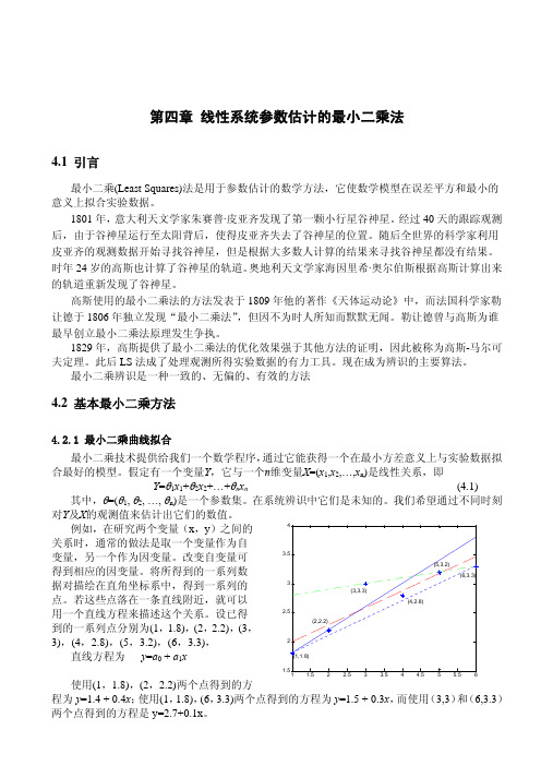
从图中可看到,前两条线都仅能满足两个点的要求,而对其它点的误差都很大,其 6 个点的 误差平方累计分别为 0.49 和 0.42。第三条线能满足三个点的要求,但误差平方累计更大,为 1.58。 显然我们需要找到一条更为理想的直线来取得较小的误差。例如图中的红色短划线,它的方程 为 y=1.697 + 0.294x,误差平方累计为 0.25。这条线是怎样得到的呢?它是用最小二乘法得到的。
z
−2
,在其输入端加入 M 序列输入后
所得到的输出输入数据见下表,请利用这些数据辨识出系统的传递函数的系数。
k
1
2
3
4
5
6
7
8
9
10
输入 u
1
0
1
1
0
0
1
1
1
0
输出 y -0.45 -0.01
1.15
2.56
1.92
-0.30 -0.80 0.91 2.92 2.40
解: 已知系统阶数 n=2,有 4 个未知数。将式(4.4)展开 y(k) = −a1 y(k −1) − a2 y(k − 2) + b0u(k) + b1u(k −1) 根据要求,观测次数 N>2n+1,取 N 为 6,k=3
最小二乘法概述

最小二乘法一、简介最小二乘法,又称最小平方法,是一种数学技术。
它通过最小误差的平方和寻找数据函数的最佳匹配。
最小二乘法是提供“观测组合”的主要工具之一,它依据对某事件的大量观测而获得“最佳”结果或“最可能”表现形式。
如已知两变量为线性关系bx a y +=,对其进行)2(>n n 次观测而获得n 对数据。
若将这n 对数据代入方程求解a ,b 之值则无确定解。
最小二乘法提供了一个求解方法,其基本思想就是寻找“最接近”这n 个观测点的直线。
最小二乘法不仅是19世纪最重要的统计方法,而且还可以称为数理统计学之灵魂。
相关回归分析、方差分析和线性模型理论等数理统计学的几大分支都以最小二乘法为理论基础。
作为其进一步发展或纠正其不足而采取的对策,不少近现代的数理统计学分支也是在最小二乘法基础上衍生出来的。
最小二乘法之于数理统计学,有如微积分之于数学,这并非夸张之辞。
统计学应用的几个分支如相关分析、回归分析、方差分析和线性模型理论等,其关键都在于最小二乘法的应用不少现代的统计学研究是在此法的基础上衍生出来,作为其进一步发展或纠正其不足之处而采取的对策,如回归分析中一系列修正最小二乘法而产生的估计方法等就是最好的例子。
二、创立思想勒让德在先驱者解线性方程组的基础上,以整体的思想方法创立了最小二乘法;高斯由寻找随机误差函数为突破,以独特的概率思想导出了正态分布,详尽地阐述了最小二乘法的理论依据。
最小二乘法(OLSE)的思想就是要使得观测点和估计点的距离平方和达到最小,在各方程的误差之间建立一种平衡,从而防止某一极端误差,对决定参数的估计值取得支配地位,有助于揭示系统的更接近真实的状态。
这里的“二乘”指的是用平方来度量观测点与估计点的远近,“最小”指的是参数的估计值要保证各个观测点与估计点的距离的平方和达到最小。
三、原理设一组数据(,)i i x y (1,2,,)i n = ,现用近似曲线)(x y ϕ=拟合这组数据,“拟合得最好”的标准是所选择的()x ϕ在i x 处的函数值()i x ϕ(1,2,,)i n = 与i y (1,2,,)i n = 相差很小,即偏差(也称残差)()i i x y ϕ-(1,2,,)i n = 都很小.一种方法是使偏差之和()1ni i i x y ϕ=⎡⎤⎣⎦∑-很小来保证每个偏差都很小.但偏差有正有负,在求和的时候可能相互抵消.为了避免这种情况,还可使偏差的绝对值之和()1||ni i i x y ϕ=-∑为最小.但这个式子中有绝对值符号,不便于分析讨论.由于任何实数的平方都是正数或零,因而我们可选择使“偏差平方和21ni i i x y ϕ=-∑[()]最小”的原则来保证每个偏差的绝对值都很小,从而得到最佳拟合曲线y =()x ϕ.这种“偏差平方和最小”的原则称为最小二乘原则,而按最小二乘法原则拟合曲线的方法称为最小二乘法或称最小二乘曲线拟合法.一般而言,所求得的拟合函数可以使不同的函数类,拟合曲线()x ϕ都是由m 个线性无关函数()1x ϕ,()2x ϕ ,…, ()m x ϕ的线性组合而成,即()()()()1122m m x a x a x a x ϕϕϕϕ=+++…)1(-<n m ,其中1a ,2a ,…,m a 为待定系数.线性无关函数()1x ϕ,()2x ϕ ,…()m x ϕ,称为基函数,常用的基函数有: 多项式:1,x , 2x ,…,m x ;三角函数: sin x ,sin 2x ,…,sin mx ;指数函数:x x x m e e e λλλ,,,21 ,x λ2e,…,x λme.最小二乘法又称曲线拟合,所谓“ 拟合” ,即不要求所作的曲线完全通过所有的数据点,只要求所得的近似曲线能反映数据的基本趋势,它的实质是离散情况下的最小平方逼近.四、运用曲线拟合做最小二乘法 1 一元线性拟合已知实测到的一组数据(,)i i x y (1,2,,)i n = ,求作这组数据所成的一元线性关系式.设线性关系式为y a bx =+,求出a 和b 即可.法一:即要满足则)(令,0,0,,12=∂∂=∂∂--=∑=bsa sb a bx a y s ni i i ,则,a b 要满足s a ∂∂=0,sb∂∂=0.即 11()()ni i i n i i ii sy a bx a s y a bx x b==∂⎧--⎪⎪∂⎨∂⎪--⎪∂⎩∑∑=-2=0=-2=0化简得112111n n i i i i nn ni i i i i i i b a x y n n a x b x x y =====⎧⎪⎪⎨⎪⎪⎩∑∑∑∑∑1+=+= 从中解出1112211111n n n i i i ii i i n n i i i i n n i ii i n x y x yb n x x b a y x n n =======⎧⎪⎪⎪⎛⎫ ⎪⎨⎝⎭⎪⎪⎪⎩∑∑∑∑∑∑∑-=-=- (1) 法二:将i x ,i y 代入y a bx =+得矛盾方程组1122n y a bx y a bx y a bx n=+⎧⎪=+⎪⎨⎪⎪=+⎩ (2) 令A =12111n x x x ⎛⎫ ⎪⎪ ⎪ ⎪⎝⎭ ,B =12n y y y ⎛⎫⎪ ⎪ ⎪ ⎪⎝⎭,则(2)式可写成b B A a ⎛=⎫⎪⎝⎭,则对应的正规方程组为TTa b A B A A ⎛=⎫ ⎪⎝⎭,所以a b ⎛⎫ ⎪⎝⎭=1()T TA A AB -,其中A 称为结构矩阵,B 称为数据矩阵,T A A 称为信息矩阵,TA B 称为常数矩阵.2 多元线性拟合设变量y 与n 个变量1x ,2x ,…,n x (1n ≥)内在联系是线性的,即有如下关系式∑=+=nj j j x a a y 10,设j x 的第i 次测量值为ij x ,对应的函数值为i y (1,2,,)i m = ,则偏差平方和为s ='220111()()mm ni i i i ij i i j y y y a a x ===-=--∑∑∑,为了使s 取最小值得正规方程组011001111011202020m n i j ij i j m n i j ij i i j m n i j ij in i j ns y a a x a s y a a x x a s y a a x x a ======⎧∂⎛⎫=---=⎪ ⎪∂⎝⎭⎪⎪∂⎛⎫=---=⎪⎪∂⎨⎝⎭⎪⎪⎪∂⎛⎫=---=⎪ ⎪∂⎝⎭⎩∑∑∑∑∑∑ (3) 即011101111n m mij j i j i i mn m mik ij ik jik i i j i i ma x a y x a x x a x y =======⎧⎛⎫+= ⎪⎪⎝⎭⎪⎨⎛⎫⎪+= ⎪⎪⎝⎭⎩∑∑∑∑∑∑∑1,2,,k n = . (4) 将实验数据(,)i i x y 代入(4)式,即得m a a a ,,,10 .3 指数函数拟合科学实验得到一组数据(,)i i x y (1,2,,)i n = 时,还可以考虑用指数函数为基函数来拟合,此时设拟合函数具有形式bxy ae =(,a b 为待定系数).对上式两端取自然对数可得:ln ln y a bx =+ (9)令Y =ln y ,0ln b a =,则(9)式可转化为一元线性函数形式0Y b bx =+,此时将指数函数拟合转化成了一元线性拟合,利用一元线性拟合中的两种方法均可求出0b 和b ,继而根据0b a e =可求出a ,从而得出因变量y 与自变量x 之间的函数关系式0b bx bx y ae e +==4 对数函数拟合科学实验得到一组数据(,)i i x y (1,2,,)i n = 时,还可以考虑用对数函数为基函数来拟合,此时设拟合函数具有形式ln y a b x =+(0)x >(,a b 为待定系数).0b >时,y 随x 增大而增大,先快后慢;0b <时,y 随x 增大而减小,先快后慢.当以y 和ln x 绘制的散点图呈直线趋势时,可考虑采用对数函数描述y 与x 之间的非线性关系,式中的b 和a 分别为斜率和截距.这时令X =ln x ,就可以利用一元线性拟合的方法来求解.更一般的对数函数还可设为y =()ln a b x k ++,式中k 为一常量.五 举例例1 使电流通过2Ω的电阻,用伏特表测量电阻两端的电压V .测得数据如下表:t I /A1 2 4 6 8 10 t V /V1.83.78.212.015.820.2试用最小二乘法建立I 与V 之间的一元经验公式(有效数字保留到小数点后第3位). 解:可取一次线性关系式V a bI =+作为I 与V 之间的一元经验公式. 将数据代入得矛盾方程组1.82 3.748.2612.0815.81020.2a b a b a b a b a b a b +=⎧⎪+=⎪⎪+=⎨+=⎪⎪+=⎪+=⎩ 令1112141618110A ⎛⎫ ⎪ ⎪ ⎪= ⎪ ⎪ ⎪ ⎪ ⎪⎝⎭, 1.83.78.212.015.820.2B ⎛⎫ ⎪ ⎪ ⎪= ⎪ ⎪ ⎪ ⎪ ⎪⎝⎭,则上述矛盾方程组可写成矩阵形式0a A B b ⎛⎫-= ⎪⎝⎭由此得出其正规方程组0T T a A A A B b ⎛⎫-= ⎪⎝⎭,将数据代入即得63161.7031221442.4a b ⎛⎫⎛⎫⎛⎫-= ⎪⎪ ⎪⎝⎭⎝⎭⎝⎭,解之得0.212.032a b =-⎧⎨=⎩,故所求经验公式为0.2152.V I =-+. 例 2 在在开发一种抗过敏性的新药时,要对不同剂量的药效进行实验.10名患者各服用了该新药的一个特定的剂量.药物消失时立即纪录.观测值列于下表中.x 是剂量,y 是症状消除持续的日数.用7个不同的剂量, 其中3个剂量重复给两名患者.试给出y 与x 之间的一元经验公式(保留3位有效数字).1 2 3 4 5 6 7 8 9 10 ∑ /i x mg334566788959/i y d9 5 12 9 14 16 22 18 24 22 1512i x 9 9 16 25 36 36 49 64 64 81 389i i x y271548458496154144192198 1003解:可设y 与x 之间的经验公式为y a bx =+. 由上表可知,101i i x =∑59=,101i i y =∑151=,101i i i x y =∑1003=,1021i i x =∑389=,2101i i x =⎛⎫ ⎪⎝⎭∑3481= 再由(1)式可求得,1010101112101021110101003591512.7410389348110i i i ii i i i i i i x y x y b x x =====-⨯-⨯===⨯-⎛⎫- ⎪⎝⎭∑∑∑∑∑10101111 2.7415159 1.0710101010i i i i b a y x ===-=⨯-⨯=-∑∑所以y 与x 之间的经验公式为 1.07 2.74y x =-+.最小二乘法能将从实验中得出的一大堆看上去杂乱无章的数据中找出一定的规律,拟合成一条曲线来反映所给数据特点。
最小二乘法(OLS)的原理解析
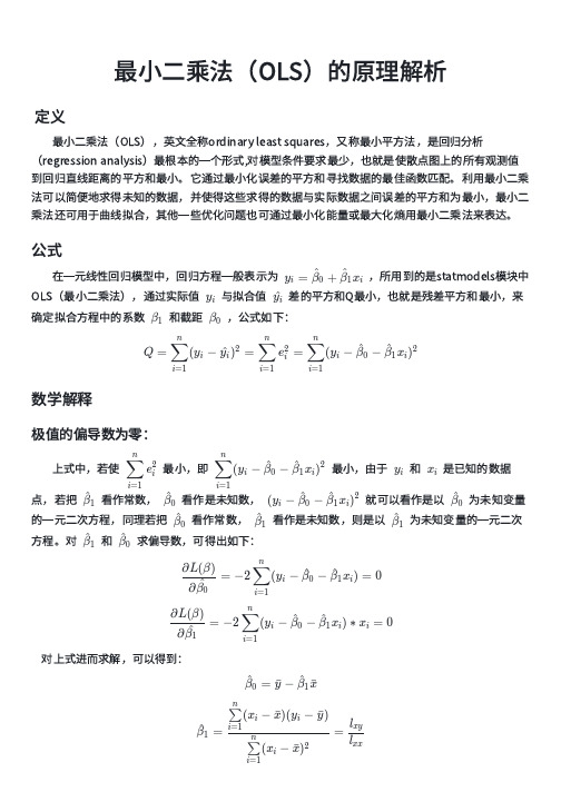
定义
最小二乘法(OLS),英文全称ordinary least squares,又称最小平方法,是回归分析 (regression analysis)最根本的一个形式,对模型条件要求最少,也就是使散点图上的所有观测值 到回归直线距离的平方和最小。它通过最小化误差的平方和寻找数据的最佳函数匹配。利用最小二乘 法可以简便地求得未知的数据,并使得这些求得的数据与实际数据之间误差的平方和为最小,最小二 乘法还可用于曲线拟合,其他一些优化问题也可通过最小化能量或最大化熵用最小二乘法来表达。
公式
在一元线性回归模型中,回归方程一般表示为
yi
=
β^0
+
β^ x 1 i
,所用到的是statmodels模块中
OLS(最小二乘法),通过实际值 yi 与拟合值 y^i 差的平方和Q最小,也就是残差平方和最小,来
确定拟合方程中的系数 β1 和截距 β0 ,公式如下:
n
n
∑
( xi
)2
−
(
∑
xi
)2
i=1
i=1
n
n
n
n
(∑
xi2
)(
∑
yi
)
−
(∑
xi)(∑
xiyi
)
β^ = i=1
0
i=1 n
i=1
i=1
n
n
∑
( xi
)2
−
(
∑
线性参数的最小二乘法处理

W1、 +1″, +10″, +1″, +12″,
W2、 +6″, +4″,
W3、
W4„
Wn
+2″ , -3″ , +4″ +12″, +4″ +3″, +4″
+12″, +12″, +12″
W12
2
12
W22
2 2
W32
32
最小值
3
即 ∑(PW2)=(P1W21)+(P2W22)+(P3W32)
的测量结果 yi 最接近真值,最为可靠,即: yi=∠i+Wi 由于改正数 Wi 的二次方之和为最小,因此称为最小二乘法。 二 最小二乘法理 现在我们来证明一下,最小二乘法和概率论中最大似然方法(算术平均值方法) 是一致的。 (一)等精度测量时 (1)最大似然方法 设 x1,x2„xn 为某量 x 的等精度测量列,且服从正态分布,现以最大似然法和最小 二乘法分别求其最或是值(未知量的最佳估计量) 在概率论的大数定律与中心极限定理那一章我们讲过,随着测量次数的增加,测 量值的算术平均值也稳定于一个常数,即
2 i 1
n
曾给出: vi2
i 1
n
n n 1 n 2 ,由此可知 x vi2 / i2 为最小,这就是最小二乘法的基本 i n i 1 i 1
含义。引入权的符号 P ,最小二乘法可以写成下列形式:
Pv
i 1
n
2 i i
最小
在等精度测量中, 1 2 ... , P1 P2 ... Pn 即: 最小二乘法可以写成下列形式:
第十八讲全面最小二乘法

Y
V H ,其中σ 1 ≥ σ 2 ≥ ≥ σ r > 0 。又设 0 m×n σ 1 Vn (s < r ) 则 U σs 0 m×n
z∈C rankz = s F
min X − Y= X −Z F m×n
H
首先来考虑 F-范数。设 Pm×n = UQV ,U、V 分别为 m 阶、n 阶酉
r
r
n
1 i= r +1 j =
∑ ∑ tij
m
n
2
对任意 Z 矩阵而言,各 tij 之间完全独立,则 X − Z 于零的。但是 rank ( Z )= s < r 。故 X − Z
F
F
是可能等
不可能为零。详细论证
F
可知 tij = 0(i ≠ j ), tii = 0(i > s ), tii = σ i (i = 1, 2,, s ) 时, X − Z 小 下 面 仅 考 虑 在 实 际 应 用 中 非 常 常 见 的 一 种 情 况 : A ∈ Cn
14
= min ∆ F =
显然满足
rank ( C +∆ ) =n
rank ( C +∆ )< n +1
min
C − (C + ∆ )
F
min
= C− ( C + ∆ ) σ n+1
0 H ∆ =U 0 V σ + n 1 O
15
定理 2: 设σ n +1 为 C 的 n-k+1 重奇异值,且 vk +1 , vk + 2 , vn +1 相应的为
线性回归之最小二乘法
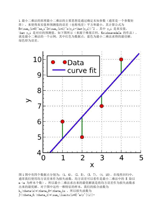
1.最小二乘法的原理最小二乘法的主要思想是通过确定未知参数(通常是一个参数矩阵),来使得真实值和预测值的误差(也称残差)平方和最小,其计算公式为E=\sum_{i=0}^ne_i^2=\sum_{i=1}^n(y_i-\hat{y_i})^2 ,其中 y_i 是真实值,\hat y_i 是对应的预测值。
如下图所示(来源于维基百科,Krishnavedala 的作品),就是最小二乘法的一个示例,其中红色为数据点,蓝色为最小二乘法求得的最佳解,绿色即为误差。
图1图中有四个数据点分别为:(1, 6), (2, 5), (3, 7), (4, 10)。
在线性回归中,通常我们使用均方误差来作为损失函数,均方误差可以看作是最小二乘法中的 E 除以m(m 为样本个数),所以最小二乘法求出来的最优解就是将均方误差作为损失函数求出来的最优解。
对于图中这些一维特征的样本,我们的拟合函数为h_\theta(x)=\theta_0+\theta_1x ,所以损失函数为J(\theta_0,\theta_1)=\sum_\limits{i=0}^m(y^{(i)}-h_\theta(x^{(i)}))^2=\sum_\limits{i=0}^m(y^{(i)}-\theta_0-\theta_1x^{(i)})^2 (这里损失函数使用最小二乘法,并非均方误差),其中上标(i)表示第 i 个样本。
2.最小二乘法求解要使损失函数最小,可以将损失函数当作多元函数来处理,采用多元函数求偏导的方法来计算函数的极小值。
例如对于一维特征的最小二乘法, J(\theta_0,\theta_1) 分别对 \theta_0 , \theta_1 求偏导,令偏导等于 0 ,得:\frac{\partial J(\theta_0,\theta_1)}{\partial\theta_0}=-2\sum_\limits{i=1}^{m}(y^{(i)}-\theta_0-\theta_1x^{(i)}) =0\tag{2.1}\frac{\partial J(\theta_0,\theta_1)}{\partial\theta_1}=-2\sum_\limits{i=1}^{m}(y^{(i)}-\theta_0-\theta_1x^{(i)})x^{(i)} = 0\tag{2.2}联立两式,求解可得:\theta_0=\frac{\sum_\limits{i=1}^m(x^{(i)})^2\sum_\limits{i=1}^my^{(i)}-\sum_\limits{i=1}^mx^{(i)}\sum_\limits{i=1}^mx^{(i)}y^{(i)}}{m\sum_\limits{i=1}^m(x^{(i)})^2-(\sum_\limits{i=1}^mx^{(i)})^2} \tag{2.3}\theta_1=\frac{m\sum_\limits{i=1}^mx^{(i)}y^{(i)}-\sum_\limits{i=1}^mx^{(i)}\sum_\limits{i=1}^my^{(i)}}{m\sum_\limits{i=1}^m(x^{(i)})^2-(\sum_\limits{i=1}^mx^{(i)})^2} \tag{2.4}对于图 1 中的例子,代入公式进行计算,得: \theta_0 = 3.5, \theta_1=1.4,J(\theta) = 4.2 。
最小二乘法求最短路径

最小二乘法求最短路径
最小二乘法是一种常用的数学方法,用于求解最短路径问题。
在
最短路径问题中,我们需要找到从起点到终点的路径,使得路径上的
总权值最小。
最小二乘法的思想是通过最小化路径上各个节点的误差平方和,
来确定最优路径。
具体而言,我们首先将问题转化为一个线性方程组,其中方程的个数等于路径上的节点数减去1。
然后,我们使用最小二乘法的公式来计算方程组的最优解。
最小二乘法首先构建一个矩阵A,其中每行对应一个方程,每列
对应一个节点。
矩阵A的元素表示两个节点之间的权值。
同时,还构
建一个列向量b,其元素为每个方程右侧的常数项。
然后,通过求解线性方程组 A^T * A * x = A^T * b ,得到解向量x,其中x的每个分
量表示路径上相应节点的权值。
最小二乘法可以使用多种数值计算方法来求解线性方程组,如高
斯消元法、QR分解、SVD分解等。
根据具体的问题和数据特点,可以
选用适合的数值计算方法,以获得最优的计算结果。
最小二乘法在求解最短路径问题时具有以下优点:(1)能够充
分考虑路径上各个节点之间的权值关系,从而寻找最优的路径;(2)
能够处理带有噪声或不完全数据的情况,提高路径计算的鲁棒性;(3)计算过程相对简单,适用于大规模问题的求解。
总之,最小二乘法是一种有效的数学方法,能够求解最短路径问题,并在实际应用中取得良好的效果。
线性系统参数估计的最小二乘方法

un (1) un (2) un ( N )
从而 ˆ ( X T X )1 X T y 如何推广到 MIMO 系统?
8
2. 非线性系统的辨识
y(k ) a0 a1u (k ) a2u 2 (k ) e(k )
选取
x1 ( k ) u (k )
得新解
ˆ(k 1) [ X T (k 1) X (k 1)]1 X T (k 1) y (k 1)
12
其中
X (k ) y (k ) , y (k 1) , X (k 1) T x (k 1) y (k 1)
20
辅助变量法
y (k ) ai y (k i ) biu (k i ) e(k )
i 1 i 1 n n
传统做法是由
X T X X T y X T e
得到
ˆ ( X T X )1 X T y ( X T X )1 X T e ,
ˆ。 如果 X 与 e 不相关,则 E ( )
i 1 i 1 i 1 n n n
令 A(q 1 ) 1 aq i , B(q ) bi q i ,则系统写成
i 1 i 1
n
n
A(q 1 ) y (k ) B(q 1 )u (k ) e(k )
其中
n
e(k ) A(q 1 ) (k )
引入变白滤波器
e( N ) 将进入ˆ 而使它偏离
2. 如 N 2n ,此时观测方程个数大于参数个数,这是一个解超 定方程问题,可取
ˆ(i )) 2 J ( N ) ( y (i ) T (i )
(完整版)5线性参数的最小二乘法处理(精)

一、等精度测量线性参数的LSM处理的正规方 程。
❖ 线性参数的误差方程式为:
l1 a11x1 a12 x2 ... a1t xt v1
l2 a21x1 a22 x2 ... a2t xt v2
……
ln an1x1 an2 x2 ... ant xt vn
v2
第三节 精度估计
❖ 一、测量数据的精度估计
❖ (一)等精度测量数据的精度估计
❖ 对包含t个未知数的线性参数方程,进行n次独立的 等精度测量。
❖ 可以证明
❖
[V V ] ~ 2 n t
2
E[V V
2
]
n
t
❖取
s 2 v v
nt
s
v
2 i
nt
❖ V1=3-(1.28×1+0.418×2)=0.884 ❖ V2=5-(1.28×1+0.418×10)=-0.46 ❖ V3=8-(1.28×1+0.418×20)=-1.64 ❖ V4=15-(1.28×1+0.418×30)=1.18 ❖ V5=18-(1.28×1+0.418×40)=0
L
8
15
18
AT A 1052 3100024 AT L 134698
( AT
A)1
1 4616
3004 102
1502
X
( AT A)1 AT L
1 4616
3004 102
1502134698 01..42188
❖ 正规方程为: ❖ 5x+102y=49 ❖ 102x+3004y=1386 ❖ 解该方程得到 ❖ x=1.28 ❖ y=0.418
i
最小二乘法 原理

最小二乘法原理最小二乘法原理最小二乘法是一种常用的数据拟合方法,通过最小化误差的平方和来寻找最佳拟合曲线或平面。
该方法的应用非常广泛,可以用于线性回归、曲线拟合、数据平滑等问题。
最小二乘法的原理可以简单概括为:在给定的数据集中,找到一条曲线或平面,使得该曲线或平面到各个数据点的距离的平方和最小。
具体而言,最小二乘法通过以下几个步骤来实现:1. 建立模型:首先需要确定拟合模型的形式,例如线性模型、多项式模型、指数模型等。
模型的选择要基于对数据的理解和背景知识。
2. 确定目标函数:目标函数是衡量拟合曲线与数据之间误差的度量。
常用的目标函数是误差的平方和,即将每个数据点到拟合曲线的距离平方求和。
3. 最小化目标函数:通过对目标函数求导,并使导数等于零,得到目标函数的最小值点。
这个最小值点就对应着最佳的拟合曲线或平面。
4. 求解参数:根据最小化目标函数的结果,求解拟合模型中的参数。
不同的模型有不同的参数,求解方法也不同。
最小二乘法的优点在于可以得到解析解,即可以用数学公式直接求解出最佳拟合曲线或平面的参数。
这使得最小二乘法非常高效,适用于大规模数据集。
最小二乘法的应用非常广泛。
在线性回归中,可以用最小二乘法来拟合一个线性模型,从而预测因变量与自变量之间的关系。
在曲线拟合中,可以用最小二乘法来拟合一个多项式模型,从而找到最佳拟合曲线。
在数据平滑中,可以用最小二乘法来拟合一个平滑曲线,从而去除数据中的噪声。
最小二乘法也有一些限制。
首先,最小二乘法要求拟合模型是线性的,对于非线性问题可能不适用。
其次,最小二乘法对异常值比较敏感,一个异常值可能会对拟合结果产生较大影响。
此外,最小二乘法假设误差服从正态分布,如果数据不满足这个假设,拟合结果可能不准确。
为了解决这些问题,可以使用其他的拟合方法,例如非线性最小二乘法、加权最小二乘法等。
这些方法在最小二乘法的基础上进行了改进,可以适用于更复杂的拟合问题。
最小二乘法是一种简单而有效的数据拟合方法。
第三章 线性最小二乘估计
第三章 线性最小二乘估计最小二乘估计方法是以误差的平方和最小为准则,根据观测数据估计线性模型中未知参数的一种基本参数估计方法。
1794年德国数学家C.F.高斯在解决行星轨道猜测问题时首先提出最小二乘法。
它的基本思路是选择估计量使模型(包括静态或动态的,线性或非线性的)输出与实测输出之差的平方和达到最小。
这种求误差平方和的方式可以避免正负误差相抵,而且便于数学处理(例如用误差的绝对值就不便于处理)。
线性最小二乘法是应用最广泛的参数估计方法,它在理论研究和工程应用中都具有重要的作用,同时它又是许多其他更复杂方法的基础。
线性最小二乘法是最小二乘法最简单的一种情况,即模型中关于参数的函数是线性的。
假设有一测量方程为 Z (k )=q +N (k ),其中()Z k 为已知的测量数据,q 为待估计量,()N k 为测量噪声,我们可以发现()Z k 与q 的关系是线性的。
最小二乘方法会告诉我们:如果我们不知道传感器的方差,要在已知测量序列的基础上,怎么样得到q 估计的值 ˆq?假设已知其方差为2R =,我们如何应用这个方差,会得到更为准确的估计吗? 3.1 最小二乘估计方法若被估计量θ是M 维矢量,则每次观测量()Z k 和观测噪声()N k 均为矢量,线性观测方程为()()()Z k H k N k θ=+,其中()Z k ,()N k 分别为第k 次观测量和观测噪声,()H k 为观测矩阵。
若我们可以得到k 个观测,将这k 个观测也可以写成向量形式,记(1)(2)...()k Z Z Z Z k ⎛⎫ ⎪ ⎪= ⎪ ⎪⎝⎭ (1)(2)...()k H H H H k ⎛⎫ ⎪ ⎪= ⎪ ⎪⎝⎭ (1)(2)...()k N N N N k ⎛⎫ ⎪ ⎪= ⎪ ⎪⎝⎭(3.1) 则上式可写为k k k Z H N θ=+。
要求构造的估计量θ∧使性能指标()()()Tk k k k J Z H Z H θθθ∧∧∧=-- (3.2)达到最小,称这种估计为最小二乘估计,记为()LS k θ∧。
线性参数的最小二乘法处

最小二乘法
v1= l1-y1 v2= l2-y2 , yn为最小二乘估计量 …. ….. vn= ln-yn
y0与最可信赖 值?Βιβλιοθήκη 一、最小二乘法原理 A
直接求得 。
B
有利于减小随机误差,方程组 有冗余,采用最小二乘原理求 。
C
讨论:
D
最小二乘原理:
E
最可信赖值应使残余误差平方和最小。
为了获得更可靠的结果,测量次数总要多于未知参数的数目
待求量
误差方程
测得值
如为精密测定1号、2号和3号电容器的电容量
组合测量基本概念
优点:精度较高。组合形式越多(n越大),测量结果的精度就越高。
缺点:工作量大
应用:在精密测量工作中有十分重要的地位,如标准器的检定。
组合测量基本概念
【例题】
则最小二乘估计量 的标准差为
02
已知
01
若测量数据 ,不存在系统误差和粗大误差,相互独立,且服从正态分布,其标准差为
则各测量结果 出现于相应真值附近 区域内的概率分别为:
各误差相互独立,由概率乘法定理,各测量数据同时分别出现在相应区域的概率应为:
例题 5-1
X 的最佳估计值
第二节 正规方程
例5.1 已知铜棒的长度和温度之间具有线性关系: ,为 。为获得0℃时铜棒的长度 和铜的线膨胀系数 ,现测得不同温度下铜 棒的长度,如下表,求 , 的最可信赖值。
10
20
25
30
40
45
2000.36
2000.72
由最小二乘法求最佳解 系数矩阵A--------误差方程,(测量方程) 测量值矩阵L------直接测得 权矩阵P 例题 5-2 X 的最佳估计值
最小二乘法线性详细说明.ppt

3. 回归方程的精度和相关系数
用最小二乘法确定a, b存在误差。 总结经验公式时,我们初步分析判断所假定
的函数关系是正确,为了解决这些问题,就 需要讨论回归方程的精度和相关性。 为了估计回归方程的精度,进一步计算数据
点 xi,yi 偏离最佳直线y=a+bx的大小,我们 引入概念——剩余标准差 s ,它反映着回
一种可能是各数据点与该线偏差较小,一种可能是各数据 点与该线偏差较大。
当R 1时,s 减小,一般的数据点越靠近最佳值两旁。两
变量间的关系线性相关,可以认为是线性关系,最佳直线 所反应的函数关系也越接近两变量间的客观关系。同时还 说明了测量的精密度高。
当条“R 最佳1时”,直线s 增。大然,而根,据数数据据点点与的“分最布佳,”也直许线能的得偏到差一过
14
根据二元函数求极值法,把③式对a和b分 别求出偏导数。得:
n
v2 i
i1
a n
2yi a bxi
4
v2 i
i1 2
b
yi a bxi xi
15
令④等于零,得:
n
n
yi na b xi 0
i1 n
i1
n
n
5
yixi
i1
a xi i1
b
x2 i
i1
0
解方程,得:
而且: b 1.993 0.006
31
第二节 二元线性回归
已知函数形式(或判断经验公式的函数形式)为 y a b1x1 b2x2
式中,均为独立变量,故是二元线性回归。 若有实验数据:
x1 x11, x12,......... .x1n x2 x21, x22,......... .x2n
glm 最小二乘法

glm 最小二乘法glm是广义线性模型(Generalized Linear Model)的缩写,最小二乘法是glm中的一种参数估计方法。
最小二乘法是一种通过最小化观测值与模型预测值之间的残差平方和来估计模型参数的方法。
最小二乘法是统计学中常用的参数估计方法之一,它可以用于解决线性回归问题。
线性回归是一种用于建立自变量和因变量之间线性关系的回归分析方法。
在线性回归中,我们希望找到一条直线,使得该直线与观测数据点的残差平方和最小。
最小二乘法通过最小化残差平方和来寻找最优拟合直线的参数。
最小二乘法的基本思想是,通过最小化残差平方和来求解模型参数。
在线性回归中,我们假设因变量Y与自变量X之间存在线性关系,即Y = β0 + β1X + ε,其中β0和β1是模型的参数,ε是误差项。
我们的目标是通过观测数据来估计β0和β1的值,从而得到最优拟合直线。
最小二乘法通过最小化残差平方和来估计模型参数。
残差是观测值与模型预测值之间的差异,残差平方和则是所有观测值的残差平方的和。
最小二乘法的思想是,通过调整模型参数,使得残差平方和最小。
具体地,我们可以通过对残差平方和对模型参数求导,然后令导数等于零,求解方程组得到最优参数估计。
最小二乘法适用于线性回归模型,当模型中存在非线性关系时,最小二乘法的估计结果可能不准确。
为了解决这个问题,可以使用广义线性模型(glm)。
广义线性模型是线性回归模型的一种扩展,它允许因变量与自变量之间存在非线性关系。
广义线性模型通过引入链接函数和矩阵乘积来描述因变量与自变量之间的关系,从而使模型能够适用于更广泛的数据类型。
最小二乘法是glm中的一种参数估计方法,它是一种通过最小化残差平方和来估计模型参数的方法。
最小二乘法适用于线性回归模型,当模型中存在非线性关系时,可以使用广义线性模型来解决。
广义线性模型通过引入链接函数和矩阵乘积来描述因变量与自变量之间的关系,从而使模型能够适用于更广泛的数据类型。
最小二乘法的原理和应用

最小二乘法的原理和应用1. 原理最小二乘法是一种最常用的参数估计方法,用于拟合数据点与理论模型之间的误差。
它通过最小化误差的平方和来确定模型参数的最佳估计值。
在最小二乘法中,我们假设数据点服从一个线性模型,即y = mx + b其中,y是因变量,x是自变量,m和b是待求的参数。
我们希望找到最优的m和b,使得模型的预测值与实际观测值之间的误差最小。
最小二乘法的核心思想是将误差平方化,即将每个数据点的误差差值平方,并将所有的差值平方求和。
通过最小化这个平方差和,我们可以得到最优的参数估计值。
2. 应用最小二乘法在各个领域中都有广泛的应用。
以下是一些常见的应用示例:2.1 线性回归最小二乘法在线性回归中被广泛使用。
线性回归是一种统计分析方法,用于确定两个变量之间的线性关系。
通过最小二乘法,我们可以估计线性回归模型中的斜率和截距,从而预测因变量的值。
2.2 数据拟合最小二乘法还可以用于数据拟合。
通过选择适当的模型和参数,最小二乘法可以拟合数据点,并生成一个描述数据行为的数学模型。
这对于预测未来的数据点或分析数据的趋势非常有价值。
2.3 图像处理最小二乘法在图像处理中也有应用。
例如,在图像平滑和去噪方面,最小二乘法可以用于拟合图像上的像素值,并通过消除噪声来提高图像的质量。
2.4 物理建模在物理建模中,最小二乘法可以用于确定物理系统的参数。
通过测量物理系统的输入和输出,并使用最小二乘法,我们可以估计出系统的参数,以便更好地理解和预测系统的行为。
3. 实现步骤最小二乘法的实现步骤如下:1.收集数据:首先,需要收集一组包含自变量和因变量的数据。
2.建立模型:根据问题的要求,选择适当的模型。
例如,在线性回归中,我们选择了y = mx + b的线性模型。
3.计算预测值:通过代入自变量的值,并使用模型中的参数,计算预测值。
4.计算误差:将预测值与实际观测值进行比较,并计算误差。
误差可以通过求差值的平方来计算。
5.求解参数:通过最小化误差的平方和,可以得到最优的参数估计值。
- 1、下载文档前请自行甄别文档内容的完整性,平台不提供额外的编辑、内容补充、找答案等附加服务。
- 2、"仅部分预览"的文档,不可在线预览部分如存在完整性等问题,可反馈申请退款(可完整预览的文档不适用该条件!)。
- 3、如文档侵犯您的权益,请联系客服反馈,我们会尽快为您处理(人工客服工作时间:9:00-18:30)。
1 35.69
0
1 7.02
0
−0.49 0.12 0.86 0.30 −0.91 0.30
8 · 38
BIT
×
H.B.Ma
2. The Pseudo-Inverse
Least-Squares
Key Point: Pseudo-Inverse Solves
least-squares estimation problems minimum-norm control problems
3 · 38
BIT
×
H.B.Ma
1. The Key Points of This Section
Least-Squares
Important Facts
null(AT ) = range(A)⊥ easy via the SVD: because if the SVD of A is A = U ΣV T then range(A) = span{u1 , . . . , ur } also the SVD of AT is A T = V ΣT U T so null(AT ) = span{ur+1 , . . . , un }
2 T = xT AT Ax − 2ymeas Ax + ymeas 2
differentiate with respect to x and set to zero
T 2xT AT A − 2ymeas A=0
so the optimum x is xopt = (AT A)−1 AT ymeas
11 · 38
10 · 38
BIT
×
H.B.Ma
3. Estimation and Least-Squares
Least-Squares
Using Differentiation
The residual is r = Ax − ymeas which we would like to minimize. So r
1. The Key Points of This Section
Least-Squares
1
The Key Points of This Section
estimation problems: given ymeas , find the least-squares solution x, that minimizes ymeas − Ax control problems: given ydes , find the minimum-norm x that satisfies ydes = Ax the SVD gives a computational approach it also gives useful information even when important assumptions don.t hold – estimation: usually need A skinny and full rank – control: usually need A fat and full rank it gives us quantitative information about the usefulness of the solutions
OUTLINE
1 The Key Points of This Section 2 The Pseudo-Inverse 3 Estimation and Least-Squares 4 Control and Minimum-Norm Solutions 5 Matrices Without Full Rank 6 Matlab and the Pseudo-Inverse 7 History of Least Squares 3 6 10 23 31 32 33
Linear System Theory:
Least Squares Hongbin Ma mathmhb@ School of Automation Beijing Instititue of Technology October 18, 2012 Beijing, China
Mainly based on S. Lall’s slides Made with mslide package in MTEX.
13 · 38
BIT
×
H.B.Ma
3. Estimation and Least-Squares
Least-Squares
Pseudo-Inverse Approach
if A is skinny and full rank then AT A is invertible and A† = (AT A)−1 AT ˆΣ ˆV T , to see this, notice that the thin SVD of A is A = U where V is square and orthogonal, so ˆΣ ˆ 2V T AT A = V U and ˆΣ ˆ −2 V T V Σ ˆU ˆT = V Σ ˆ −1 U ˆ T = A† (AT A)−1 AT = V U
BIT
×
H.B.Ma
3. Estimation and Least-Squares
Least-Squares
Geometric Approach
pick as estimate xopt ; by orthogonality Axopt − ymeas ⊥ range(A) which holds if and only if Axopt − ymeas → null(AT ) which holds if and only if AT (Axopt − ymeas ) = 0
Properties of The Pseudo-Inverse
if A is invertible, then A† = A−1 A is m × n ⇐ A† is n × m (A† )† = A (AT )† = (A† )T (λA)† = λ−1 A† for λ = 0 caution: in general, (AB )† = B † A†
BIT
×
H.B.Ma
3. Estimation and Least-Squares
Least-Squares
Effects of Noise on Estimation
Suppose we measure ymeas = Ax + w and we use estimator B with BA = I . xest = Bymeas If w ≤ 1, then the estimate lies in the ellipsoid xest → {x + Bw| w ≤ 1} because xest = B (Ax + w) = x + Bw. Picking B = A† gives semiaxis directions vi and −1 semiaxis lengths σi , worst error e = 1/σmin (A)
7 · 38
BIT
×
H.B.Ma
2. The Pseudo-Inverse
Least-Squares
Example
the thin svd: −0.49 0.30 35.69 0 = 0.12 −0.91 0 7.02 0.86 0.30 pseudo-inverse: 0.33 0.38 0.31 0.20 † A = 0.79 −0.11 0.39 −0.53 −0.15 −0.73 0.33 0.31 0.79 0.39 −0.15 0.38 0.20 −0.11 −0.53 −0.73
14 · 38
BIT
×
H.B.Ma
3. Estimation and Least-Squares
Least-Squares
Left-Inverse Property
when A is skinny and full rank, A† is a left-inverse for A A† A = I
5 · 38
ห้องสมุดไป่ตู้BIT
×
H.B.Ma
2. The Pseudo-Inverse
Least-Squares
2
The Pseudo-Inverse
ˆΣ ˆV T the thin SVD is A = U
here ˆ is square, diagonal, positive definite Σ ˆ and V ˆ are skinny, orthonormal columns U the pseudo-inverse of A is ˆΣ ˆ −1 U ˆT A† = V it is computed using the SVD
6 · 38 BIT × H.B.Ma
2. The Pseudo-Inverse
Least-Squares
Example
rank 2 matrix: −5 −5 −14 −8 1 A = −1 0 4 5 4 11 10 24 11 −6 the full svd:
−0.49 0.30 0.82 35.69 0 0 0 0 = 0.12 −0.91 0.41 0 7.02 0 0 0 × 0.86 0.30 0.41 0 0 000 0.33 0.31 0.79 0.39 −0.15 0.38 0.20 −0.11 −0.53 −0.73 0.25 −0.86 0.36 −0.25 0.01 0.45 −0.26 −0.47 0.67 −0.25 0.69 0.22 −0.14 −0.25 0.62