FLAC_3D快速入门(手册翻译版——一米)
FLAC_3D快速入门(手册翻译版——一米)
FLAC_3D快速入门(手册翻译版——一米)FLAC3D3.0版本3.0中文手册一米固定y范围y -0.1 0.1固定y范围y 7.9 8.1固定z范围z -0.1 0.1应用szz -1e6范围z 7.9 8.1 hist unb hist总成xvel 3 4 4 hist总成zdisp 0 0 8 step 1500;求解(可使用步进命令或求解命令)模型开始时,最大不平衡力为1MN。
经过1500步计算,最大不平衡力下降到大约270牛顿。
通过绘制第一个历史变量图,我们可以看到最大不平衡力接近“0”。
输入以下命令,在FLAC3D中显示图2.15中的图像:图表hist 1输入:图表hist 2图表hist 3. 43。
FLAC3D3.0版本3.0中文手册一米图2.15最大不平衡力记录可以分别看到记录节点的速度记录图(见图 2.16)和位移记录图(见图2.16)。
. 44。
FLAC3D3.0版本3.0中文手册一米2.17).从图2.16中可以看出,速度值已经接近“0”;我们还可以在图2.17中看到位移值已经接近固定值。
上述条件都说明了一件事:模型已经达到初始平衡状态。
图2.16节点(3,4,4)x向速度记录图图2.17节点(0,0,8)z向位移记录图. 45。
FLAC3D3.0版本3.0中文手册一米如果用户希望FLAC3D在计算结束时自动控制(当最大不平衡力小于某个极限值时),他可以使用求解而不是步进命令。
在上面的例子中,步骤1500可以由sovle代替。
这一次,计算将在1650停止。
如果也记录了上述变量的历史记录,则绘制的图表应与前三个图表大体相同。
如果我们使用求解命令,默认情况下,系统通过最大不平衡力的比值来控制计算过程。
当最大不平衡力与初始施加的节点力的平均值之比小于1×10⁻⁵时,计算将停止。
在输入求解命令之前,我们也可以通过输入以下命令来手动设置该比率:在这里设置机械比率= f,f是用户给出的比率限制。
flac3d实用教程

高效的求解器
FLAC3D采用显式有限差分法,计算效率高, 能够处理大规模的计算问题。
安装步骤及注意事项
2. 解压安装包到指定目录。
1. 从官方网站下载 FLAC3D安装包。
安装步骤
01
03 02
安装步骤及注意事项
3. 运行安装程序,按照提示完成安装过程。
4. 安装完成后,启动FLAC3D软件。
安装步骤及注意事项
FLAC3D支持导入多种格式的外部几何模型,如STL、IGES等。通过导入功能,可以快速将复 杂几何体导入FLAC3D中进行后续分析。
利用内置工具创建简单几何体
对于简单的几何形状,如立方体、圆柱体等,可以直接使用FLAC3D内置的创建工具进行建 模。
布尔运算构建复杂模型
FLAC3D提供布尔运算功能,支持对多个几何体进行并集、交集、差集等操作,以构建更为 复杂的几何模型。
水文地质领域应用案例剖析
地下水渗流模拟
FLAC3D可以模拟地下水在复杂地 质条件下的渗流过程,为地下水 资源的开发和保护提供决策支持。
水库大坝渗流分析
利用FLAC3D对水库大坝进行渗流 分析,可以评估大坝的安全性和 稳定性,为水库运行管理提供科 学依据。
岩溶地区水文地质
模拟
FLAC3D可以模拟岩溶地区的水文 地质过程,包括岩溶发育、地下 水流动等,为岩溶地区的水资源 管理和工程建设提供参考。
它广泛应用于岩土工程、地质工程、水利工程 等领域,用于分析土壤、岩石和其他地质材料 的力学行为。
FLAC3D基于显式有限差分法,能够高效处理 大变形和非线性问题,特别适用于模拟地震、 滑坡、隧道开挖等复杂地质工程问题。
软件特点与优势
强大的后处理功能
软件提供了丰富的后处理工具,如等值线 图、矢量图、动画演示等,方便用户直观 地查看和分析计算结果。
FLAC3D基础知识介绍
FLAC 3D基础知识介绍一、概述FLAC(Fast Lagrangian Analysis of Continua)由美国Itasca公司开发的。
目前,FLAC有二维和三维计算程序两个版本,二维计算程序V3.0以前的为DOS版本,V2.5版本仅仅能够使用计算机的基本内存64K),所以,程序求解的最大结点数仅限于2000个以内。
1995年,FLAC2D已升级为V3.3的版本,其程序能够使用护展内存。
因此,大大发护展了计算规模。
FLAC3D是一个三维有限差分程序,目前已发展到V3.0版本。
FLAC3D的输入和一般的数值分析程序不同,它可以用交互的方式,从键盘输入各种命令,也可以写成命令(集)文件,类似于批处理,由文件来驱动。
因此,采用FLAC程序进行计算,必须了解各种命令关键词的功能,然后,按照计算顺序,将命令按先后,依次排列,形成可以完成一定计算任务的命令文件。
FLAC3D是二维的有限差分程序FLAC2D的护展,能够进行土质、岩石和其它材料的三维结构受力特性模拟和塑性流动分析。
调整三维网格中的多面体单元来拟合实际的结构。
单元材料可采用线性或非线性本构模型,在外力作用下,当材料发生屈服流动后,网格能够相应发生变形和移动(大变形模式)。
FLAC3D采用的显式拉格朗日算法和混合-离散分区技术,能够非常准确的模拟材料的塑性破坏和流动。
由于无须形成刚度矩阵,因此,基于较小内存空间就能够求解大范围的三维问题。
三维快速拉格朗日法是一种基于三维显式有限差分法的数值分析方法,它可以模拟岩土或其他材料的三维力学行为。
三维快速拉格朗日分析将计算区域划分为若干四面体单元,每个单元在给定的边界条件下遵循指定的线性或非线性本构关系,如果单元应力使得材料屈服或产生塑性流动,则单元网格可以随着材料的变形而变形,这就是所谓的拉格朗日算法,这种算法非常适合于模拟大变形问题。
三维快速拉格朗日分析采用了显式有限差分格式来求解场的控制微分方程,并应用了混合单元离散模型,可以准确地模拟材料的屈服、塑性流动、软化直至大变形,尤其在材料的弹塑性分析、大变形分析以及模拟施工过程等领域有其独到的优点。
Flac3D使用手册
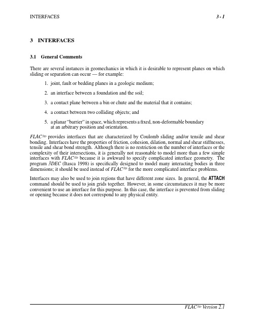
3INTERFACES3.1General CommentsThere are several instances in geomechanics in which it is desirable to represent planes on which sliding or separation can occur—for example:1.joint,fault or bedding planes in a geologic medium;2.an interface between a foundation and the soil;3.a contact plane between a bin or chute and the material that it contains;4.a contact between two colliding objects;and5.a planar“barrier”in space,which represents afixed,non-deformable boundaryat an arbitrary position and orientation.FLAC3D provides interfaces that are characterized by Coulomb sliding and/or tensile and shear bonding.Interfaces have the properties of friction,cohesion,dilation,normal and shear stiffnesses, tensile and shear bond strength.Although there is no restriction on the number of interfaces or the complexity of their intersections,it is generally not reasonable to model more than a few simple interfaces with FLAC3D because it is awkward to specify complicated interface geometry.The program3DEC(Itasca1998)is specifically designed to model many interacting bodies in three dimensions;it should be used instead of FLAC3D for the more complicated interface problems. Interfaces may also be used to join regions that have different zone sizes.In general,the ATTACH command should be used to join grids together.However,in some circumstances it may be more convenient to use an interface for this purpose.In this case,the interface is prevented from sliding or opening because it does not correspond to any physical entity.3.2FormulationFLAC 3D represents interfaces as collections of triangular elements (interface elements),each of which is defined by three nodes (interface nodes).Interface elements can be created at any location in space.Generally,interface elements are attached to a zone surface face;two triangular interface elements are defined for every quadrilateral zone face.Interface nodes are then created automatically at every interface element vertex.When another grid surface comes into contact with an interface element,the contact is detected at the interface node,and is characterized by normal and shear stiffnesses,and sliding properties.Each interface element distributes its area to its nodes in a weighted fashion.Each interface node has an associated representative area.The entire interface is thus divided into active interface nodes representing the total area of the interface.Figure 3.1illustrates the relation between interface elements and interface nodes and the representative area associated with an individual node.elementinterfaceFigure 3.1Distribution of representative areas to interface nodesIt is important to note that interfaces are one-sided in FLAC 3D .(This differs from the formulation of two-sided interfaces in two-dimensional FLAC (Itasca 2000).)It may be helpful to think of FLAC 3D interfaces as “shrink-wrap”that is stretched over the desired surface,causing the surface to become sensitive to interpenetration with any other face with which it may come into contact.The fundamental contact relation is defined between the interface node and a zone surface face,also known as the target face .The normal direction of the interface force is determined by the orientation of the target face.During each timestep,the absolute normal penetration and the relative shear velocity are calculated for each interface node and its contacting target face.Both of these values are then used by the interface constitutive model to calculate a normal force and a shear-force vector.The constitutive model is defined by a linear Coulomb shear-strength criterion that limits the shear force acting at an interface node,normal and shear stiffnesses,tensile and shear bond strengths,and a dilation angle that causes an increase in effective normal force on the target face after the shear-strength limit is reached.By default,pore pressure is used in the interface effective stress calculation.This option can be activated/deactivated using the command INTERFACE i effective=on/off.Figure3.2 illustrates the components of the constitutive model acting at interface node(P).Figure3.2Components of the bonded interface constitutive modelThe normal and shear forces that describe the elastic interface response are determined at calculation time(t+ t)using the following relations.F(t+ t)n=k n u n A+σn A(3.1)F(t+ t) si =F(t)si+k s u(t+(1/2) t)siA+σsi Awhere F(t+ t)n is the normal force at time(t+ t)[force];F(t+ t)si is the shear force vector at time(t+ t)[force];u n is the absolute normal penetration of the interface nodeinto the target face[displacement];u si is the incremental relative shear displacement vector[displacement];σn is the additional normal stress added due to interface stressinitialization[force/displacement];k n is the normal stiffness[stress/displacement];k s is the shear stiffness[stress/displacement];σsi is the additional shear stress vector due to interface stressinitialization;andA is the representative area associated with the interface node[length2].The inelastic interface logic works in the following way:(1)Bonded interface—The interface remains elastic if stresses remain below the bondstrengths:there is a shear bond strength as well as a tensile bond strength.The nor-mal bond strength is set using the tension interface property keyword.The commandINTERFACE n prop sbratio=sbr sets the shear bond strength to sbr times the normal bondstrength.The default value of sbratio(if not given)is100.0.The bond breaks if either theshear stress exceeds the shear strength,or the tensile effective normal stress exceeds thenormal strength.Note that giving sbratio alone does not cause a bond to be established;the tensile bond strength must also be set.(2)Slip while bonded—An intact bond,by default,prevents all yield behavior(slip andseparation).There is an optional property switch(bslip)that causes just separationto be prevented if the bond is intact(but allows shear yield,under the control of thefriction and cohesion parameters,using abs(F n)as the normal force).The command toallow/disallow slip for a bonded interface segment isINTER n PROP bslip=onbslip=offThe default state of bslip(if not given)is off.(3)Coulomb sliding—A bond is either intact or broken.If it is broken,then the behaviorof the interface segment is determined by the friction and cohesion(and of course thestiffnesses).This is the default behavior,if bond strengths are not set(zero).A brokenbond segment cannot take effective tension(which may occur under compressive normalforce,if the pore pressure is greater).The shear force is zero(for a non-bonded segment)if the effective normal force is tensile or zero.The Coulomb shear-strength criterion limits the shear force by the following relation.F smax=cA+tanφ(F n−pA)(3.2)where c is the cohesion[stress]along the interface;φis the friction angle[degrees]of the interface surface;andp is pore pressure(interpolated from the target face),provided the keywordeffective=off has not been issued for the interface.If the criterion is satisfied(i.e.,if|F s|≥F smax),then sliding is assumed to occur,and |F s|=F smax,with the direction of shear force preserved.During sliding,shear displacement may cause an increase in the effective normal stress on the joint,according to the relation:σn:=σn+|F s|o−F smaxAk s tanψk n(3.3)whereψis the dilation angle[degrees]of the interface surface;and|F s|o is the magnitude of shear force before the above correction is made.On printout(PRINT interface n prop tens),the value of tension denotes if a bond is intact or broken (or not set)—non-zero or zero,respectively.The normal and shear forces calculated at the interface nodes are distributed in equal and opposite directions to both the target face and the face to which the interface node is connected(the host face). Weighting functions are used to distribute the forces to the gridpoints on each face.The interface stiffnesses are added to the accumulated stiffnesses at gridpoints on both sides of the interface,in order to maintain numerical stability.Interface contacts are detected only at interface nodes,and contact forces are transferred only at interface nodes.The stress state associated with a node is assumed to be uniformly distributed over the entire representative area of the node.Interface properties are associated with each node; properties may vary from node to node.By default,the effect of pore pressure is included in the interface calculation by using effective stress as the basis for the slip condition.(The interface pore pressure is interpolated from the target face.)This applies either in CONFIGfluid mode,or if pore pressures are assigned with the WATER table or INITIAL pp command without specifying CONFIGfluid.The user can switch options for interface i by using the command INTERFACE i effective=on/off.By default,in the FLAC3D logic,fluidflow—saturated or unsaturated—is carried across an interface,provided the interface keyword maxedge is not used for that particular interface.The permeable interface option can be deactivated/reactivated for interface i by using the command INTERFACE i perm=on/off.Note that if the keyword maxedge is used,and perm is on for a particular interface,a warning is issued to inform the user that this interface will be considered as impermeable tofluidflow.(Note that, forfluidflow calculation only,a mechanical model must be present.Also,the command CYCLE 0with SET mech on should be used to initialize the weighting factors used to transferfluidflow information across the interface.)No pressure drop normal to the joint and no influence of normal displacement on pore pressure are calculated.Also,flow offluid along the interface is not modeled.3.3Creation of Interface GeometryInterfaces are created with the INTERFACE command.For cases in which an interface is required between two separate grids in the model,the command INTERFACE i face range...should be used to attach an interface to one of the grid surfaces.This command generates interface elements for interface i along all surface zone faces with a center point that fall within a specified range.Any surfaces on which an interface is to be created must be generated initially with some separation between the adjacent surfaces;it must be possible to specify an existing surface in order to create the interface elements.(Also,a gap must be specified between the two grids because the grid generator will automatically merge surface gridpoints if they are created at the same location in space.)By default,two interface elements are created for each zone face.The number of interface elements can be increased by using the command INTERFACE i maxedge v.*This causes all interface elements with edge lengths larger than v to subdivide into smaller elements until their lengths are smaller than v.This command can be used to increase the resolution and decrease arching of forces in portions of a model that have large contrasts in zone size across an interface.The following rules should be followed when using interface elements in FLAC3D.1.If a smaller surface area contacts a larger surface area(e.g.,a small block restingon a large block),the interface should be attached to the smaller region.2.If there is a difference in zone density between two adjacent grids,the interfaceshould be attached to the grid with the greater zone density(i.e.,the greaternumber of zones within the same area).3.The size of interface elements should always be equal to or smaller than thetarget faces with which they will come into contact.If this is not the case,theinterface elements should be subdivided into smaller elements.4.Interface elements should be limited to grid surfaces that will actually comeinto contact with another grid.A simple example illustrating the procedure for interface creation is provided in Example3.1.The example is a block specimen containing a single joint dipping at an angle of45◦.Example3.1Creating a model with a dipping joint;Create Basegen zone brick size333&p0(0,0,0)p1(3,0,0)p2(0,3,0)p3(0,0,1.5)&p4(3,3,0)p5(0,3,1.5)p6(3,0,4.5)p7(3,3,4.5)group Base*Note that if CONFIGfluid is invoked,and perm is on for a particular interface,specifying maxedge for that interface will automatically make it impermeable.Do not specify maxedge ifflow across the interface is desired.;Create Top-1unit high for initial spacinggen zone brick size333&p0(0,0,2.5)p1(3,0,5.5)p2(0,3,2.5)p3(0,0,7)&p4(3,3,5.5)p5(0,3,7)p6(3,0,7)p7(3,3,7)group Top range group Base not;;Create interface elements on the top surface of the baseinterface1face range plane norm(-1,0,1)origin(1.5,1.5,3)dist0.1;plot create view_intplot add surfaceplot add interface redplot showpause;;Lower top to complete geometryini z add-1.0range group Topsave int.savFigure3.3shows the grid before the interface is created.Two sub-grid groups are defined:a Base grid,and a Top grid.Figure3.4shows the model with the interface elements attached to the Base grid.Figure3.5shows thefinal geometry with the sub-grids moved together.A uniaxial compression test with this model is described later in Section3.4.3.Figure3.3Initial geometry before creation of the interfaceFigure3.4Interface elements addedFigure3.5Final geometry3.4Choice of Material PropertiesAssignment of material properties(particularly stiffnesses)to an interface depends on the way in which the interface is used.Three possibilities are common.The interface may be:1.an artificial device to connect two sub-grids together;2.a real interface that is stiff compared to the surrounding material,but which canslip and perhaps open in response to the anticipated loading.(This case alsoencompasses the situation in which stiffnesses are unknown or unimportant,but where slip and/or separation will occur—e.g.,flow of frictional materialin a bin);or3.a real interface that is soft enough to influence the behavior of the system(e.g.,a joint with soft clayfilling or a dyke containing heavily fractured material).These cases are examined in detail.3.4.1Interface Used to Join Two Sub-gridsIf possible,sub-grids should be joined with the ATTACH command.It is more computationally-efficient to use ATTACH than INTERFACE to join sub-grids.See Section3.2.1.2in the User’s Guide, for a description of,and restrictions on,the ATTACH command.Under some circumstances it may be necessary to use an interface to join two sub-grids.This type of interface is assigned high strength properties with the INTERFACE command,thus preventing any slip or separation.(This is the equivalent of a“glued”interface in FLAC.)Shear and normal stiffnesses must also be provided;values of friction and cohesion are not needed.It is tempting (particularly for people familiar withfinite element methods)to give a very high value for these stiffnesses to prevent movement on the interface.However,FLAC3D does“mass scaling”(see Section1.1.2.6)based on stiffnesses—the response(and solution convergence)will be very slow if very high stiffnesses are specified.It is recommended that the lowest stiffness consistent with small interface deformation be used.A good rule-of-thumb is that k n and k s be set to ten times the equivalent stiffness of the stiffest neighboring zone.The apparent stiffness(expressed in stress-per-distance units)of a zone in the normal direction ismax K+43Gz min(3.4)where K&G are the bulk and shear moduli,respectively;andz min is the smallest width of an adjoining zone in the normal direction—seeFigure3.6.The max[]notation indicates that the maximum value over all zones adjacent to the interface is to be used(e.g.,there may be several materials adjoining the interface).InterfaceFigure3.6Zone dimension used in stiffness calculationTo illustrate the approach,consider Figure3.7,in which two sub-grids of unequal zoning are joined by the commands in Example3.2and are loaded by a pressure on the left-hand part of the upper surface:Example3.2Joining two sub-gridsgen zone brick size444p00,0,0p14,0,0p20,4,0p30,0,2gen zone brick size884p00,0,3p14,0,3p20,4,3p30,0,5inter1face range z 2.9,3.1inter1prop kn300e9ks300e9tens1e10SBRATIO=1ini z add-1.0range z 2.9,5.1model elasprop bulk8e9shear5e9fix z range z-.1.1fix x range x-.1.1fix x range x 3.9 4.1fix y range y-.1.1fix y range y 3.9 4.1apply szz-1e6range z 3.9 4.1x0,2y0,2hist unbalsolvesave join.savThe value of(K+4G/3)is15GPa,and the minimum zone size adjacent to the interface is 0.5m.Hence,we choose both shear stiffness and normal stiffness to be150×109/0.5—i.e., k n=k s=3×10¹¹Pa/m.The resulting contours of z-displacement are shown in Figure3.8.Compare this result to that for a single grid,shown in Figure3.7in the User’s Guide.This plot is at the same scale and contour intervals as Figure3.8.The two plots are almost identical,which indicates that the interface does not affect the behavior to any great extent.The prescription given in Eq.(3.4)is reasonable if the materials on the two sides of the interface are similar,and variations of stiffness occur only in the lateral directions.However,if the material on one side of the interface is much stiffer than that on the other,then Eq.(3.4)should be applied to the softer side.In this case,the deformability of the whole system is dominated by the soft side;making the interface stiffness ten times the soft-side stiffness will ensure that the interface has minimal influence on system compliance.Figure3.7Two unequal sub-grids joined by an interfaceFigure3.8Vertical displacement contours—two joined grids3.4.2Real Interface—Slip and Separation OnlyIn this case,we simply need to provide a means for one sub-grid to slide and/or open relative to another sub-grid.The friction(and perhaps cohesion,dilation,and tensile strength)is important, but the elastic stiffness is not.The approach of Section3.4.1is used here to determine k n and k s. However,the other material properties are given real values(see Section3.4.3for advice on choice of properties).As an example,we can allow slip in a bin-flow problem,as shown in Figure3.9,corresponding to the datafile in Example3.3.The bond strengths are not set(i.e.,they default to zero);the interface stiffnesses are set to approximately ten times the equivalent stiffness of the neighboring zones.Figure3.9Flow of frictional material in a“bin”Example3.3Slip in a bin-flow problem;Create Material Zonesgen zone brick size555&p0(0,0,0)p1(3,0,0)p2(0,3,0)p3(0,0,5)&p4(3,3,0)p5(0,5,5)p6(5,0,5)p7(5,5,5) gen zone brick size555p0(0,0,5)edge 5.0group Material;Create Bin Zonesgen zone brick size155&p0(4,1,0)p1add(3,0,0)p2add(0,3,0)&p3add(2,0,5)p4add(3,6,0)p5add(2,5,5)&p6add(3,0,5)p7add(3,6,5)gen zone brick size155&p0(6,1,5)p1add(1,0,0)p2add(0,5,0)&p3add(0,0,5)p4add(1,6,0)p5add(0,5,5)&p6add(1,0,5)p7add(1,6,5)gen zone brick size515&p0(1,4,0)p1add(3,0,0)p2add(0,3,0)&p3add(0,2,5)p4add(6,3,0)p5add(0,3,5)&p6add(5,2,5)p7add(6,3,5)gen zone brick size515&p0(1,6,5)p1add(5,0,0)p2add(0,1,0)&p3add(0,0,5)p4add(6,1,0)p5add(0,1,5)&p6add(5,0,5)p7add(6,1,5)group Bin range group Material not;Create named range synonymsrange name=Bin group Binrange name=Material group Material;Assign models to groupsmodel mohr range Materialmodel elas range Bin;Create interface elementsint1face ran plane ori(4,0,0)nor(-5,0,2)dist0.01z(0,5)y(1,6) int2face ran plane ori(0,4,0)nor(0,-5,2)dist0.01z(0,5)x(1,6) int1face ran x 5.9 6.1y16z510int2face ran x16y 5.9 6.1z510int1maxedge0.55int2maxedge0.55;Move bin toward materialini x add-1.0range Binini y add-1.0range Bin;Assign propertiesprop shear1e8bulk2e8fric30range Materialprop shear1e8bulk2e8range Binini den2000int1prop ks2e9kn2e9fric15int2prop ks2e9kn2e9fric15;Assign Boundary Conditionsfix x range x-0.10.1any x 5.9 6.1anyfix y range y-0.10.1any y 5.9 6.1anyfix z range z-0.10.1Bin;Monitor historieshist unbalhist gp zdisp(6,6,10)hist gp zdisp(0,0,10)hist gp zdisp(0,0,0);Settingsset largeset grav0,0,-10;Cyclingstep4000save bin.sav3.4.3All Properties Have Physical SignificanceIn this case,properties should be derived from tests on real joints*(suitably scaled to account for size effect),or from published data on materials similar to the material being modeled.However, the comments of Section3.4.1also apply here with respect to the maximum stiffnesses that are reasonable to use.If the physical normal and shear stiffnesses are less than ten times the equivalent stiffness of adjacent zones,then there is no problem in using physical values.If the ratio is much more than ten,the solution time will be significantly longer than for the case in which the ratio is limited to ten,without much change in the behavior of the system.Serious consideration should be given to reducing supplied values of normal and shear stiffnesses to improve solution efficiency. There may also be problems with interpenetration if the normal stiffness,k n,is very low.A rough estimate should be made of the joint normal displacement that would result from the application of typical stresses in the system(u=σ/k n).This displacement should be small compared to a typical zone size.If it is greater than,say,10%of an adjacent zone size,then there is either an error in one of the numbers,or the stiffness should be increased if calculations are to be done in large-strain mode.Joint properties are conventionally derived from laboratory testing(e.g.,triaxial and direct shear tests).These tests can supply physical properties for joint friction angle,cohesion,dilation angle, and tensile strength,as well as joint normal and shear stiffnesses.The joint cohesion and friction angle correspond to the parameters in the Coulomb strength criterion†described in Section3.2. Values for normal and shear stiffnesses for rock joints typically can range from roughly10to100 MPa/m for joints with soft clay in-filling,to over100GPa/m for tight joints in granite and basalt. Published data on stiffness properties for rock joints are limited;summaries of data can be found in Kulhawy(1975),Rosso(1976),and Bandis et al.(1983).Approximate stiffness values can be back-calculated from information on the deformability and joint structure in the jointed rock mass and the deformability of the intact rock.If the jointed rock mass is assumed to have the same deformational response as an equivalent elastic continuum,then relations can be derived between jointed rock properties and equivalent continuum properties. For uniaxial loading of rock containing a single set of uniformly spaced joints oriented normal to the direction of loading,the following relation applies.1=1r +1n(3.5)*“Joint”is used here as a generic term.†The Coulomb yield surface provides a reasonable approximation for joint strength for most engi-neering calculations.More complex joint models are available which include,for example,effects of continuous yielding and displacement weakening.For analysis with other joint models,the user is referred to UDEC(Itasca1996).ork n=E E rs(E r−E)(3.6)where E=rock mass Young’s modulus;E r=intact rock Young’s modulus;k n=joint normal stiffness;ands=joint spacing.A similar expression can be derived for joint shear stiffness:k s=G G rs(G r−G)(3.7)where G=rock mass shear modulus;G r=intact rock shear modulus;andk s=joint shear stiffness.The equivalent continuum assumption,when extended to three orthogonal joint sets,produces the following relations:E i=1r+1i ni−1(i=1,2,3)(3.8)G ij=1G r+1s i k si+1s j k sj−1(i,j=1,2,3)(3.9)Several expressions have been derived for two-and three-dimensional characterizations and multiple joint sets.References for these derivations can be found in Singh(1973),Gerrard(1982(a)and (b)),and Fossum(1985).Published strength properties for joints are more readily available than stiffness properties.Sum-maries can be found,for example,in Jaeger and Cook(1979),Kulhawy(1975),and Barton(1976). Friction angles can vary from less than10◦for smooth joints in weak rock,such as tuff,to over 50◦for rough joints in hard rock,such as granite.Joint cohesion can range from zero to values approaching the compressive strength of the surrounding rock.It is important to recognize that joint properties measured in the laboratory typically are not rep-resentative of those for real joints in thefield.Scale dependence of joint properties is a major question in rock mechanics.Often,the only way to guide the choice of appropriate parameters is by comparison to similar joint properties derived fromfield tests.However,field test observations are extremely limited.Some results are reported by Kulhawy(1975).The following example illustrates an application of the interface logic to simulate the physical response of a rock joint subjected to normal and shear loading.The model represents a direct shear test,which consists of a single horizontal joint that isfirst subjected to a normal confining stress, and then to a unidirectional shear displacement.Figure3.10shows the model.Figure3.10Direct shear test modelFirst,a normal stress of10MPa is applied that is representative of the confining stress acting on the joint.A horizontal velocity is then applied to the top sub-grid to produce a shear displacement along the interface.For demonstration purposes,we only apply a small shear displacement of less than2mm to this model.The average normal and shear stresses,and normal and shear displacements along the joint,are measured with a FISH function.With this information we can determine the shear strength and dilation that are produced.The datafile for this test is contained in Example3.4.Example3.4Direct shear testtitleDirect shear testgen zone brick size12110p0406p11606p2416p34011 gen zone brick size20110p12000p2010p3005range name bot z05range name top z611interface1face range z5int1prop ks4e4kn4e4fric30dil6;tension1e10bslip=onini z add-1.0range top;plo surf lorange interface white axes blackmodel eprop bulk45e3sh30e3fix x y z range z0fix x range x0fix x range x20apply nstress-10range z10step0plot contour szz interface white axes blacksolvesave dsta.savini xvel5e-7range topfix xvel range topdef ini_jdispvalnd=0.0count=0.0p_in=i_node_head(i_head)loop while p_in#nullif in_ztarget(p_in)#null thenvalnd=valnd+in_pen(p_in)count=count+ 1.0end_ifp_in=in_next(p_in)end_loopnjdisp0=valnd/countendini_jdispdef sstavvalns=0.0valss=0.0valsd=0.0valnd=0.0count=0.0p_in=i_node_head(i_head)loop while p_in#nullif in_ztarget(p_in)#null thenvalns=valns+in_nstr(p_in)*in_area(p_in)valss=valss+in_sstr(p_in,1)*in_area(p_in)valsd=valsd+in_sdisp(p_in,1)valnd=valnd+in_pen(p_in)count=count+ 1.0end_ifp_in=in_next(p_in)end_loopsstav=valss/(12.0*1.0)nstav=valns/(12.0*1.0)sjdisp=valsd/countnjdisp=valnd/count-njdisp0endhist ns1hist sstav nstav sjdisp njdispini xdis0ydis0zdis0step2500save dst.savplot his-1vs-3pauseplot his-4vs-3pauseretThe average shear stress versus shear displacement along the joint is plotted in Figure3.11,and the average normal displacement versus shear displacement is plotted in Figure3.12.These plots indicate that joint slip occurs for the prescribed properties and conditions.The loading slope in Figure3.11is initially linear and then becomes nonlinear as interface nodes begin to fail until a peak shear strength of approximately5.8MPa is reached.As indicated in Figure3.12,the joint begins to dilate when the interface nodes begin to fail in shear.。
flac3D_快速入门(2)

快 速 入 门(GETTING STARTED)版本:flac3d 3.0版(FTD127)翻译:一米2009.06声 明现在市面上关于FLAC3D软件的教材寥寥无几,在学习的过程中,主要还是参考软件本身的使用手册,虽然读英文版手册有些吃力,但是它论述非常详细,我觉得是用户最好的教材。
我在边看手册的时候边做了翻译,目前为止翻译完成了本部分的内容(略去了部分内容和例子),还翻译了命令手册的前半部分内容,等翻译完成了,也会和网友共享,但是像本人这类英语水平一般的人做这样的翻译工作是比较辛苦的,我也不确定是否有毅力完成命令手册下半部分的内容。
虽然这样的工作比较艰难,但我觉得还是学到了不少东西,手册是最原始,最翔实的基础教材,看明白了手册,运用软件才会游刃有余。
由于本人专业水平和英语能力的限制,存在问题是在所难免的,有的地方甚至可能曲解了原意。
考虑到时间因素,译文的措辞没有细细斟酌,还请网友谅解。
如果发现译文中的错误,还请广大读者斧正。
一米2 快速入门这一部分将向初次使用flac3d的用户介绍软件的基本使用方法。
主要有以下内容:软件的安装与启动;用软件分析解决问题的步骤,在每一步的操作中,都有简单例题来说明该步骤具体是如何操作的。
如果你对软件比较熟悉,但是现在很少用它来处理问题,那么这部分的内容(尤其2.7节)能很好的帮你回顾软件操作的要点。
本部分3.3节全面详细的介绍了如何进行问题的求解。
Flac3d支持命令驱动和图形菜单驱动两种模式*。
在本手册中大部分的算例都采用了命令驱动模式。
我们认为这种模式能给用户提供操作软件最清晰的思路。
在1.1节中我们就已经提到了命令驱动模式使得flac3d在分析求解工程问题时成为了一个功能强大的“多面手”。
然而这种模式让新用户,或者长时间未接触软件的老用户用起来有点不那么容易。
命令行必须用键盘输入,可以直接输入到软件的命令窗口,或者先保存为数据文件,再通过软件的相关命令进行读取。
FLAC3D常见命令与使用技巧
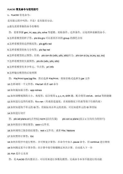
FLAC3D常见命令与使用技巧1、FLAC3D常见命令:是有限元程序吗答:不是!是有限差分法。
2.最先需要掌握的命令有哪些答:需要掌握gen, ini, app, plo, solve等建模、初始条件、边界条件、后处理和求解的命令。
3.怎样看模型的样子答:plo blo gro可以看到不同的group的颜色分布4.怎样看模型的边界情况答:plo gpfix red5.怎样看模型的体力分布答:plo fap red6.怎样看模型的云图答:位移:plo con dis (xdis, ydis, zdis)应力:plo con sz (sy, sx,sxy, syz, sxz)7.怎样看模型的矢量图答:plo dis (xdis, ydis, zdis)8.怎样看模型有多少单元、节点答:pri info9.怎样输出模型的后处理图答:File/Print type/Jpg file,然后选择File/Print,将保存格式选择为jpe文件10.怎样调用一个文件答:File/call或者call命令10.如何施加面力答:app nstress11.如何调整视图的大小、角度答:综合使用x, y, z, m, Shift键,配合使用Ctrl+R,Ctrl+Z等快捷键12.如何进行边界约束答:fix x ran(约束的是速度,在初始情况下约束等效于位移约束)13.如何知道每个单元的ID答:用鼠标双击单元的表面,可以知道单元的ID和坐标14.如何进行切片答:plo set plane ori (点坐标) norm (法向矢量) plo con sz plane (显示z方向应力的切片)15.如何保存计算结果答:save +文件名.16.如何调用已保存的结果答:rest +文件名;或者File / Restore17.如何暂停计算答:Esc18.如何在程序中进行暂停,并可恢复计算答:在命令中加入pause命令,用continue进行继续19.如何跳过某个计算步答:在计算中按空格键跳过本次计算,自动进入下一步20. Fish是什么东西答:是FLAC3D的内置语言,可以用来进行参数化模型、完成命令本身不能进行的功能21. Fish是否一定要学答:可以不用,需要的时候查Mannual获得需要的变量就可以了允许的命令文件格式有哪些答:无所谓,只要是文本文件,什么后缀都可以23.如何调用一些可选模块答:config dyn (fluid, creep, cppudm)24 .如何在圆柱体四周如何施加约束条件答:可以用fix ... ran cylinder end1 end2 radius r1 cylinder end1 end2radius r2 not,其中r225.如何能把一个PLOT的图像数据导出来以便用其他软件绘图答:用set log on命令,把数据导出来,转到excel里处理一下,然后用surfer或者什么作图软件绘制就行了。
1FLAC 3D基本介绍

1.基本介绍1.1.概述FLAC 3D是一个三维显式有限差分程序,主要应用于工程力学计算。
程序基于二维FLAC程序中已经建好的数值方程式。
FLAC 3D将FLAC的分析能力拓展到三维,用于模拟三维土体、岩体或其他材料的力学特性,尤其是达到屈服极限的塑性流变特性。
用户通过调整多面体单元的三维网格结构,来拟合要被建模的物体的实际形状。
每个单元体根据既定的线形/非线性的应力/应变规律对相应施加的力和边界约束条件作出响应。
并且当材料发生屈服流动后,网格也能够适应变形和移动(大变形模式)。
FLAC 3D采用的显式拉格朗日算法和混合——离散分区技术能够确保材料塑性坍塌破坏和流动过程的精确模拟。
由于无须形成刚度矩阵,因此采用较小的计算资源,就能够求解大范围的三维(岩土工程)计算问题。
通过自动惯性缩放及自动阻尼,显式方程式的缺点(小时间步限制和阻尼问题)已经被克服,且不会影响到物体的原有破坏行为。
FLAC 3D为三维岩土工程问题的解决提供了一个理想的分析工具。
FLAC 3D被设计,专门为了在装有Windows98及更高的版本的操作系统的IBM兼容的微型计算机上操作。
在岩土工程方面,实际的三维模型计算可以在合理的时间内被完成。
例如,创建一个包含大约140000个单元体的模型需要128M的内存。
对于一个有10000个单元体的摩尔——库伦模型,在2.4GHz的奔腾IV微型计算机上,完成5000个计算步需要大概18分钟。
对于显式计算求解,到达平衡状态的所需求解计算步数不定,但无论什么类型的模型,这个值都大概会在3000-5000步之内。
随着浮点数计算速度的提高,以及以低代价安装附加内存的能力,用FLAC 3D解决更大的三维问题成了可能。
FLAC 3D既可以通过命令行驱动,也可以通过图案菜单驱动。
默认的命令驱动模式和Itasca其他的软件产品是一样的。
你会发现其中大部分命令都是一样的。
在FLAC 3D中,菜单驱动的图形用户界面可用于绘图,显示工作。
FLAC 7.0 手册翻译 01

1粘质土边坡的稳定性1.1问题描述在工程土力学中一个普遍的问题是粘质土边坡的稳定性。
本例中土质视为均匀的,共有三个边坡状态分析。
第一个状态:黏聚力为0的砂质边坡,边坡角大于砂土的休止角。
第二个状态:给材质赋予较小的黏聚力,重新计算边坡是否稳定。
第三个状态,水位上升,分析其对边坡的稳定性影响。
(对于含潜水面的模拟研究,可以从两个方面实现:孔隙水压分布或地下水位面。
) 1.2建模步骤1.2.1初始模型状态图 1 材料的初始赋值参数建模需要考虑以下五个方面的内容:(1)模型尺寸:计算模型范围的选取直接关系到计算结果的正确与否,范围太大,白费计算机资源,范围太小,计算结果不合实际;(2)网格数目和分布:计算模型的尺寸一旦确定,计算网格的数目也相应确定,为减少因网格划分引起的误差,网格的长宽比应不大于5,对于重点研究区域可以进行网格加密处理;(3)工程对象:对于开挖、支护工程,应在建模中进行规划,调整网格结点,安排开挖以及支护的位置等;(4)材料力学参数:根据实际工程确定本构关系,赋相应的力学参数值(5)边界条件:位移边界和力边界两种(包括模型内部出适应力和位移),在计算前应确定模型的边界状况。
采用命令生成网格模型:示例:图 2 部分命令(分号后的内容为注释语句,非命令)参考解释(摘自网络):grid 20 10模型开始建立时,设置在x方向上总的单元格数目i和模型在y方向上总的单元格数目j。
gen x1,y1 x2,y2 x3,y3 x4,y4模型总网格数目给定后,需对模型整体区域进行圈定来确定模型的尺寸,(x1,y1)、(x2,y2)、(x3,y3)和(x4,y4)分别为区域从左下角起按顺时针旋转的四点坐标。
gen xi1,yi1 xi2,yi2 xi3,yi3 xi4,yi4 i=1,n1 j=1,m1 (i区)gen xii1,yii1 xii2,yii2 xii3,yii3 xii4,yii4 i=n1,n2 j=1,m1 (ii区)(i、j为区域沿x、y方向的结点号)图 3 20×10的网格1234图 4 分配第二个区域红色线圈的范围与四条蓝色的线圈区域取交集,其机制应该还是取四个点,因为第一个点的i和j规定要值都为最小,所以最终取上图中的四个红点,围成的区域是分配的第二个区域。
flac3d入门指南
设置初始应力的弹塑性求解:
gen zon bri size 1 1 2 model mohr prop bulk 3e7 shear 1e7 c 10e3 f 15 ten 0 fix z ran z 0 fix x ran x 0 fix x ran x 1 fix y ran y 0 fix y ran y 1 ini dens 2000 ini szz -40e3 grad 0 0 20e3 ran z 0 2 ini syy -20e3 grad 0 0 10e3 ran z 0 2 ini sxx -20e3 grad 0 0 10e3 ran z 0 2 set grav 0 0 -10 solve
4、边界条件及初始条件
在FLAC3D中,包含多种边界条件,边界方位 可以任意变化,边界条件可以是速度边界、应力边 界,单元内部可以给定初始应力,节点可以给定初 始位移、速度等,还可以给定地下水位以计算有效 应力等。这众多的边界条件主要通过apply或fix命 令来进行设置。而初始条件则主要通过initial命令 来执行,对所提的这两个命令必须严格区分并了解 其差异。通常我们所计算的模型均采用力学边界, 初始条件也基本是初始地应力的输入,对此两种不 同的力,其设置存在差别,同时在计算过程中,该 二者的变化情况也各不相同。
对于这两种基本的 网格,其公共面上的 关键点的对应关系更 需校核好,否则将出 现杂乱错误的网格。
对此马蹄形隧道,其公 共面处,p0 — p0,p1—p3, p2—p2,p4—p5 , p8—p9,p10 —p11
对于对称的模型也可以采 用镜像命令:
gen zone reflect norm -1 0 0 & origin 0,0,0
对于任何形状的单元体, 其建立单元模型时关键
DEFORM-3D基本操作入门

DEFORM-3D基本操作入门QianRF前言有限元法是根据变分原理求解数学物理问题的一种数值计算方法。
由于采用类型广泛的边界条件,对工件的几何形状几乎没有什么限制和求解精度高而得到广泛的应用。
有限元法在40年代提出,通过不断完善,从起源于结构理论、发展到连续体力学场问题,从静力分析到动力问题、稳定问题和波动问题。
随着计算机技术的发展与应用,为解决工程技术问题,提供了极大的方便。
现有的计算方法(解析法、滑移线法、上限法、变形功法等)由于材料的本构关系,工具及工件的形状和摩擦条件等复杂性,难以获得精确的解析解。
所以一般采用假设、简化、近似、平面化等处理,结果与实际情况差距较大,因此应用不普及。
有限元数值模拟的目的与意义是为计算变形力、验算工模具强度和制订合理的工艺方案提供依据。
通过数值模拟可以获得金属变形的规律,速度场、应力和应变场的分布规律,以及载荷-行程曲线。
通过对模拟结果的可视化分析,可以在现有的模具设计上预测金属的流动规律,包括缺陷的产生(如角部充不满、折叠、回流和断裂等)。
利用得到的力边界条件对模具进行结构分析,从而改进模具设计,提高模具设计的合理性和模具的使用寿命,减少模具重新试制的次数。
通过模具虚拟设计,充分检验模具设计的合理性,减少新产品模具的开发研制时间,对用户需求做出快速响应,提高市场竞争能力。
一、刚(粘)塑性有限元法基本原理刚(粘)塑性有限元法忽略了金属变形中的弹性效应,依据材料发生塑性变形时应满足的塑性力学基本方程,以速度场为基本量,形成有限元列式。
这种方法虽然无法考虑弹性变形问题和残余应力问题,但可使计算程序大大简化。
在弹性变形较小甚至可以忽略时,采用这种方法可达到较高的计算效率。
刚塑性有限元法的理论基础是Markov变分原理。
根据对体积不变条件处理方法上的不同(如拉格朗日乘子法、罚函数法和体积可压缩法),又可得出不同的有限元列式其中罚函数法应用比较广泛。
根据Markov变分原理,采用罚函数法处理,并用八节点六面体单元离散化,则在满足边界条件、协调方程和体积不变条件的许可速度场中对应于真实速度场的总泛函为:∏≈∑π(m)=∏(1,2,…,m)(1)对上式中的泛函求变分,得:∑=0(2)采用摄动法将式(2)进行线性化:=+Δun(3)将式(3)代入式(2),并考虑外力、摩擦力在局部坐标系中对总体刚度矩阵和载荷列阵,通过迭代的方法,可以求解变形材料的速度场。
Flac3D中文流体计算

Fl a C3D中文手册FLAC3D的计算模式中是否需要做孔压分析取决因此否采纳c on f ig fluid 命令。
1无渗流模式(不使用config fluid)即使不使用命令config flu i d,仍然能够在节点上施加孔压。
这种模式下,孔压将保持为常量。
假如采纳塑性本构模型的话,材料的破坏将市有效应力状态来控制、节点上的孔压分布可由i n i tia 1 pp命令或wa t er t ab 1 e命令来设定。
假如采纳water ta b 1 e命令,由程序自动计算水位线以下的静水孔压分布。
此时,必须施加流体密度(water d e nsit y )与重力(s et g rav i t y )o流体密度值与水位位置能够用命令p r i n t wa t er显示、假如水位线是由face关键字来定义的,则可用命令plot wa t er命令显示水位、这两种情况,单元的孔压都由节点孔压值平均求出,并在本构模型计算中用作有效应力。
这种计算模式下,体积力中不反映流体的出现:用户必须依照水位线以上或以下相应地指定干密度与湿密度。
使用命令prin t gp pp与p r i i nt zone pp可分不得到节点或单元孔压。
plot con t o u r p p命令可绘岀节点孔压云图。
2渗流模式(使用c onfi g f 1 uid)假如使用命令c onf i g fluid,则可进行瞬时渗流分析,孔压改变与潜水而的改变都估计出现、在co n f i g fl u id模式下,有效应力计算(静态孔压分布)与非排水计算均被执行、除此之外,还可进行全耦合分析,这种情况下,孔压改变将使固体产生变形,同时体积应变反过来影响孔压的变化。
假如采纳渗流模式,单元孔压仍由节点孔压平均求出、但这种模式,用户只能指定干密度(不论是水位以上依然以下),因为FLAC3D将流体的影响考虑到了体积力的计算中。
采纳渗流模式时,渗流模型必须施加到单元上,使用命令m o del fl_ isotropi c 模拟各向同性渗流,m o del fl_ani s otr o pi c模拟各向异性渗流,mode 1fl_nu 1 I模拟非渗透物质。
FLAC_3D快速入门(手册翻译版——一米)

快速入门(GETTING STARTED)版本:flac3d 3.0版(FTD127)翻译:一米2009.06声明现在市面上关于FLAC3D软件的教材寥寥无几,在学习的过程中,主要还是参考软件本身的使用手册,虽然读英文版手册有些吃力,但是它论述非常详细,我觉得是用户最好的教材。
我在边看手册的时候边做了翻译,目前为止翻译完成了本部分的内容(略去了部分内容和例子),还翻译了命令手册的前半部分内容,等翻译完成了,也会和网友共享,但是像本人这类英语水平一般的人做这样的翻译工作是比较辛苦的,我也不确定是否有毅力完成命令手册下半部分的内容。
虽然这样的工作比较艰难,但我觉得还是学到了不少东西,手册是最原始,最翔实的基础教材,看明白了手册,运用软件才会游刃有余。
由于本人专业水平和英语能力的限制,存在问题是在所难免的,有的地方甚至可能曲解了原意。
考虑到时间因素,译文的措辞没有细细斟酌,还请网友谅解。
如果发现译文中的错误,还请广大读者斧正。
一米2 快速入门这一部分将向初次使用flac3d 的用户介绍软件的基本使用方法。
主要有以下内容:软件的安装与启动;用软件分析解决问题的步骤,在每一步的操作中,都有简单例题来说明该步骤具体是如何操作的。
如果你对软件比较熟悉,但是现在很少用它来处理问题,那么这部分的内容(尤其2.7 节)能很好的帮你回顾软件操作的要点。
本部分3.3 节全面详细的介绍了如何进行问题的求解。
Flac3d 支持命令驱动和图形菜单驱动两种模式*。
在本手册中大部分的算例都采用了命令驱动模式。
我们认为这种模式能给用户提供操作软件最清晰的思路。
在1.1 节中我们就已经提到了命令驱动模式使得flac3d 在分析求解工程问题时成为了一个功能强大的“多面手”。
然而这种模式让新用户,或者长时间未接触软件的老用户用起来有点不那么容易。
命令行必须用键盘输入,可以直接输入到软件的命令窗口,或者先保存为数据文件,再通过软件的相关命令进行读取。
FLAC3D入门基本知识

FLAC3D入门基本知识FLAC3D一点知识点,仅以参考4、id,cid的区别id是指在整个结构中的编号,而cid是指在某一类比如说cable中的编号。
拿cable 中的一个单元来说,它既有自己在整个结构中的cd,又有自己在cable中的cid如果我设置了两个pilesel pile id=1 begin=(10.0, 1.0, 0.0) end=(10.0, 1.0, -10.0) nseg=5sel pile id=2 begin=(10.0, 3.0, 0.0) end=(10.0, 3.0, -10.0) nseg=5那么,id=1是不是代表第一根桩?第一根桩分五段,cid=1~5,那么第二根桩是cid=6~10!5、什么情况下使用set large?初始应力平衡的时候,不能用large模式。
在进行初始应力平衡时一定不要用!在进行大变形计算时,最好要用!!一般硬岩可以使用FLAC默认的小应变,如果是土体和软岩,用大应变 . 在做开挖的时候在进行原始应力平衡计算的时候是用小应变,后面的开挖以及支护的时候选用大应变.6、得到初始应力的方法:方法、可以先给一些材料参数很大的值,进行初始求解,在计算之前再将材料参数设为正常值,即可。
如在手册中给的第一个示例中就是这样做的。
下面是例子,These are only initial values that are used during the development of gravitational stresses within the body. In effect, we are forcing the body to behave elastically during the development of the initial in-situ stress state.* This prevents any plastic yield during the initial loading phase of the analysis. Gen zone brick size 6 8 8Mode mohrProp bulk 1e8 shear 0.3e8 fric 35Prop cohesion 1e10 tens 1e10 ;注意在此这个值给的很大。
FLAC3D基础介绍

GeoHohai
命令栏
18/74
菜单驱动(Plot)
GeoHohai
19/74
Case-2 一个最简单的例子
gen zon bri size 3 3 3 ;建立网格
model elas
;材料参数
prop bulk 3e8 shear 1e8
ini dens 2000
;初始条件
fix z ran z -.1 .1
GeoHohai
38/74
接触面单元的用途
岩体介质中的解理、断层、岩层面 地基与土体的接触 箱、槽及其内充填物的接触 空间中无变形的固定“障碍”
GeoHohaiΒιβλιοθήκη 39/74接触面的原理
如:井
孔隙压力,孔隙率,饱和度和流体属性的初始分 布可以用INITIAL命令或者PROPERTY命令定义。
GeoHohai
29/74
单渗流计算及渗流耦合计算
时间比例 完全耦合分析方法 孔压固定分析(有效应力分析) 单渗流得到孔压分布 无渗流计算——孔压的力学响应 流-固耦合计算
GeoHohai
PROP biot_c 0 (or INI fmod 0)
GeoHohai
33/74
无渗流计算——孔压的力学响应
不排水短期响应 两种分析方法:干法和湿法
干法:Ku=K+a2M 两种破坏形式
WATER或INI获得常孔压,不排水的c,φ (孔压改变较小) φ=0,c=cu (M>>K+4/3G)
GeoHohai
16/74
FLAC3D的前后处理
命令驱动(推荐)
程序控制 图形界面接口 计算模型输出 指定本构模型及参数 指定初始条件及边界条件,指定结构单元 指定接触面 指定自定义变量及函数(FISH) 求解过程的变量跟踪 进行求解 模型输出
Flac使用基础知识

1.sxx是指x方向的正应力,而szz是指z方向的正应力2.gp_head 结点指针循环,zone_head单元指针循环3.grad 线性梯度应力的关系4.apply施加边界条件,initial 施加初始条件。
5.dim就是dimension,尺寸。
一般指内部尺寸,比如radcyl内部的隧道的尺寸。
6.norm是表示法向量, dist是interface的厚度,norm是表示法向量与X、Y、Z交角的余旋7.检测某点的最大主应力和最小主应力:hist zone smax(smin) id …8.apply sxx 1.0 hist x_stress就是把x_stress的历史记录当成一个力施加给xstress,hist x_stress 前面的1表示1倍9.各点变形量用文件形式输出set log onset logfile gp-disp.txtset log off10.显示塑性区plo bl sta she-n 当前处于剪切破坏plo bl sta she-p 当前处于弹性,以前处于剪切破坏plo bl sta ten-n 当前处于抗拉破坏plo bl sta ten-p 当前处于弹性,以前处于抗拉破坏这跟flac3d的运算原理有关,它实际上是一个平衡计算扩散的求解过程。
与有限元的求解不同:有限元的计算是先组成总体的刚度矩阵,也就是模型有任何一个扰动,模型计算都要进行整体的应力平衡,这样很费内存,也是所有隐式计算程序都使用的方法,这不太符合实际岩体或土体的应力传播实际。
而flac3d软件是采用显式计算方法进行的编程,不用形成总体刚度矩阵,节省内存用量。
模型中的应力、位移传播、平衡过程比较符合工程实际。
以前处于塑性状态实际上是计算过程中(模型中的应力、位移传播、平衡过程中)局部平衡过程中出现的塑性状态。
在不断扩大的计算求解中可能该部位又一次调整为了弹性状态,也就是现在处于弹性状态,不过展示塑性区时也要算上该区域!11.id是指在整个结构中的编号,而cid是指在某一类比如说cable中的编号。
FLAC 3D基础知识
FLAC 3D基础知识介绍一、概述FLAC(Fast Lagrangian Analysis of Continua)由美国Itasca公司开发的。
目前,FLAC有二维和三维计算程序两个版本,二维计算程序V3.0以前的为DOS版本,V2.5版本仅仅能够使用计算机的基本内存64K),所以,程序求解的最大结点数仅限于2000个以内。
1995年,FLAC2D已升级为V3.3的版本,其程序能够使用护展内存。
因此,大大发护展了计算规模。
FLAC3D是一个三维有限差分程序,目前已发展到V3.0版本。
FLAC3D的输入和一般的数值分析程序不同,它可以用交互的方式,从键盘输入各种命令,也可以写成命令(集)文件,类似于批处理,由文件来驱动。
因此,采用FLAC程序进行计算,必须了解各种命令关键词的功能,然后,按照计算顺序,将命令按先后,依次排列,形成可以完成一定计算任务的命令文件。
FLAC3D是二维的有限差分程序FLAC2D的护展,能够进行土质、岩石和其它材料的三维结构受力特性模拟和塑性流动分析。
调整三维网格中的多面体单元来拟合实际的结构。
单元材料可采用线性或非线性本构模型,在外力作用下,当材料发生屈服流动后,网格能够相应发生变形和移动(大变形模式)。
FLAC3 D采用的显式拉格朗日算法和混合-离散分区技术,能够非常准确的模拟材料的塑性破坏和流动。
由于无须形成刚度矩阵,因此,基于较小内存空间就能够求解大范围的三维问题。
三维快速拉格朗日法是一种基于三维显式有限差分法的数值分析方法,它可以模拟岩土或其他材料的三维力学行为。
三维快速拉格朗日分析将计算区域划分为若干四面体单元,每个单元在给定的边界条件下遵循指定的线性或非线性本构关系,如果单元应力使得材料屈服或产生塑性流动,则单元网格可以随着材料的变形而变形,这就是所谓的拉格朗日算法,这种算法非常适合于模拟大变形问题。
三维快速拉格朗日分析采用了显式有限差分格式来求解场的控制微分方程,并应用了混合单元离散模型,可以准确地模拟材料的屈服、塑性流动、软化直至大变形,尤其在材料的弹塑性分析、大变形分析以及模拟施工过程等领域有其独到的优点。
(完整word版)flac命令流

1、FLAC3D常见命令:1. FLAC3D是有限元程序吗?答:不是!是有限差分法。
2。
最先需要掌握的命令有哪些?答:需要掌握gen, ini, app,plo,solve等建模、初始条件、边界条件、后处理和求解的命令. 3。
怎样看模型的样子?答:plo blo gro可以看到不同的group的颜色分布4. 怎样看模型的边界情况?答:plo gpfix red5。
怎样看模型的体力分布?答:plo fap red6。
怎样看模型的云图?答:位移:plo con dis (xdis,ydis,zdis)应力:plo con sz (sy, sx, sxy, syz,sxz)7。
怎样看模型的矢量图?答:plo dis (xdis,ydis, zdis)8。
怎样看模型有多少单元、节点?答:pri info9。
怎样输出模型的后处理图?答:File/Print type/Jpg file,然后选择File/Print,将保存格式选择为jpe文件10. 怎样调用一个文件?答:File/call或者call命令10. 如何施加面力?答:app nstress11. 如何调整视图的大小、角度?答:综合使用x, y, z, m,Shift键,配合使用Ctrl+R,Ctrl+Z等快捷键12. 如何进行边界约束?答:fix x ran (约束的是速度,在初始情况下约束等效于位移约束)13. 如何知道每个单元的ID?答:用鼠标双击单元的表面,可以知道单元的ID和坐标14。
如何进行切片?答:plo set plane ori (点坐标) norm (法向矢量)plo con sz plane (显示z方向应力的切片)15. 如何保存计算结果?答:save +文件名.16. 如何调用已保存的结果?答:rest +文件名;或者File / Restore17。
如何暂停计算?答:Esc18。
如何在程序中进行暂停,并可恢复计算?答:在命令中加入pause命令,用continue进行继续19. 如何跳过某个计算步?答:在计算中按空格键跳过本次计算,自动进入下一步20。
FLAC-3D讲义
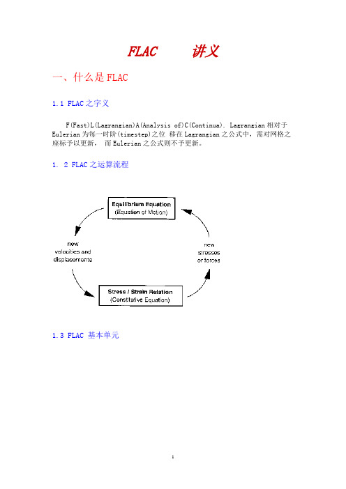
FLAC 讲义一、什么是FLAC1.1 FLAC之字义F(Fast)L(Lagrangian)A(Analysis of)C(Continua). Lagrangian相对于Eulerian为每一时阶(timestep)之位移在Lagrangian之公式中,需对网格之座标予以更新,而Eulerian之公式则不予更新。
1. 2 FLAC之运算流程1.3 FLAC 基本单元1.4 分析模式大小与RAM之关系1.5 单位1.6 正负号方向(1)应力-正号代表张力,负号代表压力(2)剪应力-详见下图,图中所示剪应力为正号(3)应变-正的应变表示伸长,负的应变代表压缩(4)剪应变-剪应变的正负号与剪应力相同(5)孔隙压力-孔隙压力永远为正(6)重力-正号的重力物质往下拉,负号的重力将物质往上提。
二、FLAC内建之组合律FLAC内建之组合律有:1.空洞模式(null model)使用于土壤被移除或开挖2.弹性模式3.塑性模式,包括a. Drucker -Prager modelb. Mohr-Coulomb modelc. ubiquitous-joint modeld. strain-hardening/softening modele. bilinear strain-hardening/softening modelf. double-yield modelg modified cam-clay model此外,另有选购(option)模式,包括:1. 动力模式(Dynamic Option)2. 热力模式(Thermal Option)3. 潜变模式 (Creep Option)使用者另可使用FISH语言去建构独特的组合律以符合所需。
三、FLAC-以命令为输入语法请查阅相关手册四、FLAC程式之使用步骤4.1 FLAC程式使用前准备步骤步骤1:依比例画出所欲分析之资料于纸上画出地点之位置、地层资料、并简标示距离及深度资料。
FLAC程序使用手册

- 1、下载文档前请自行甄别文档内容的完整性,平台不提供额外的编辑、内容补充、找答案等附加服务。
- 2、"仅部分预览"的文档,不可在线预览部分如存在完整性等问题,可反馈申请退款(可完整预览的文档不适用该条件!)。
- 3、如文档侵犯您的权益,请联系客服反馈,我们会尽快为您处理(人工客服工作时间:9:00-18:30)。
快速入门(GETTING STARTED)版本:flac3d 3.0版(FTD127)翻译:一米2009.06声明现在市面上关于FLAC3D软件的教材寥寥无几,在学习的过程中,主要还是参考软件本身的使用手册,虽然读英文版手册有些吃力,但是它论述非常详细,我觉得是用户最好的教材。
我在边看手册的时候边做了翻译,目前为止翻译完成了本部分的内容(略去了部分内容和例子),还翻译了命令手册的前半部分内容,等翻译完成了,也会和网友共享,但是像本人这类英语水平一般的人做这样的翻译工作是比较辛苦的,我也不确定是否有毅力完成命令手册下半部分的内容。
虽然这样的工作比较艰难,但我觉得还是学到了不少东西,手册是最原始,最翔实的基础教材,看明白了手册,运用软件才会游刃有余。
由于本人专业水平和英语能力的限制,存在问题是在所难免的,有的地方甚至可能曲解了原意。
考虑到时间因素,译文的措辞没有细细斟酌,还请网友谅解。
如果发现译文中的错误,还请广大读者斧正。
一米2 快速入门这一部分将向初次使用 flac3d 的用户介绍软件的基本使用方法。
主要有以下内容:软件的安装与启动;用软件分析解决问题的步骤,在每一步的操作中,都有简单例题来说明该步骤具体是如何操作的。
如果你对软件比较熟悉,但是现在很少用它来处理问题,那么这部分的内容(尤其 2.7 节)能很好的帮你回顾软件操作的要点。
本部分 3.3 节全面详细的介绍了如何进行问题的求解。
Flac3d 支持命令驱动和图形菜单驱动两种模式*。
在本手册中大部分的算例都采用了命令驱动模式。
我们认为这种模式能给用户提供操作软件最清晰的思路。
在 1.1 节中我们就已经提到了命令驱动模式使得 flac3d 在分析求解工程问题时成为了一个功能强大的“多面手”。
然而这种模式让新用户,或者长时间未接触软件的老用户用起来有点不那么容易。
命令行必须用键盘输入,可以直接输入到软件的命令窗口,或者先保存为数据文件,再通过软件的相关命令进行读取。
Flac3d 能识别超过 40 个主命令和 400 多个附属的关键词。
本部分主要包括以下内容:1 在 2.1 节,手把手的教你们如何在自己的电脑上安装和启动 flac3d 软件。
2 在 2.2 节,用一些简单的教学案例帮组用户熟悉一些常用的命令。
3 在用户建立自己的模型并进行分析计算之前,有必要先了解 flac3d 的一些基本知识。
在 2.3 节讲述了 flac3d 的基本术语;在 2.4 节主要说明了有限差分网格的定义规则;而在 2.5 节阐述了输入命令的基本句法。
4 在 2.6 节,阐述了 flac3d 的特点,比如创建、命名和使用对象,以方便用户进行问题的求解5 在 2.7 节,一步步的指导用户如何建模和分析问题,每一个步骤都分开论述,并提供简单的例子帮助用户理解。
6 2.8 节-2.10 节分别论述了系统的符号约定、单位体系和精度限制7 2.11 节说明了软件中各种类型文件的创建和使用。
8 2.12 节对图形菜单操作模式进行了简介。
*:对于初级用户来说一般图形菜单驱动模式只进行图形输出或者文件操作。
本章节的最后一部分将向用户展示如何使用图形菜单驱动模式来操作软件。
2.1 安装启动程序2.1.1 系统要求安装运行 flac3d 需要的系统最低配置如下:处理器:时钟频率至少为 1GHZ,处理器的主频越高,那么 flac3d 的计算速度将越快。
硬盘:安装软件至少需要 12MB 的硬盘空间。
如果装载了在线的用户手册,那么还需要 16MB 的空间。
(注意默认情况下,安装软件时会自动装载用户手册)。
除此之外,还需要至少 100MB 的硬盘空间来存储分析计算时生成的各种文件。
内存-启动软件至少需要 3MB 的内存。
在建模过程中,软件所占用的内存,会不断的发生变化(见表 2.1)WINDOW 操作系统还限定了软件建模时占用的内存不能超过 2GB。
显示器:推荐 1024×768 分辨率,16 位彩色显示器。
操作系统:FLAC3D 是 32 位操作系统的应用程序,所以基于 intel 技术的 WINDOWS 98 及以上操作系统均支持软件的安装和使用。
输出设备:默认情况下,系统图形会输出到系统打印机上。
也可以复制到剪贴板上,或者保存为格式化的文件,这里所说的格式包括:加强型图元文件格式和位图文件格式(PCX/BMP/JPEG)。
用户可以使用set plot 命令来指定输出的形式及格式。
2.1.2 软件的安装(略)2.1.3 组件软件的可执行文件为“F3300.EXE”。
FLAC3D 是使用 VC++ 7.0 编写的。
除了可执行程序外,还需要两套动态链接库(DLL 文件),一套用来接入和存取各种各样的图形;另一套提供内置的各种本构模型。
2.1.4 应用程序和图形处理设备在使用 FLAC3D 时,各种应用软件和图形处理设备会起到很大的辅助作用。
编辑器:任何以 ASCII 码为标准格式的文本编辑器都可以用来创建 FLAC3D 的数据文件。
但是必须要注意一些“先进”的文档编辑器(如 WordPerfect, Word 等软件),这些编辑器会把格式说明信息编译成标准输出格式,这些说明信息并不能被 FLAC3D 识别,所以导入这类文档时会出现错误。
FLAC3D 输入的数据文件必须是标准ASCII 码形式的文件。
图形输出设备:FLAC3D 支持很多种类型的图形处理设备,默认情况下,生成的图形可以用“Plot hardcopy”命令来连接到系统默认的打印机以便输出。
(或者通过 FLAC3D 主窗口中FILE 菜单栏下的print-view 来设定)“Plot clipboard”命令可以将显示的图形,存放到 WINDOWS 剪贴板上(没有任何文件生成)。
该图形接着就可以以加强型图元文件格式被粘贴到其它兼容该格式的 WINDOWS 应用程序中去。
“Set plot metafile”命令可以将图形以加强型图元格式存盘,以便作为计算的参考或日后插入到文档中去。
通过命令:Set plot +关键词(pcx, bitmap, bmp 或者jpg)可以存储为许多图像格式(pcx,bmp,jpeg 等)。
输出的这些位图的分辨率由命名行:Set plot <output type> size 来控制。
当然也可以使用Set plot avi 或者Set plot dcx 以及Set plot movie 命令将显示图形输出为视屏格式。
无论是黑白的还是彩色的 postscript 打印机,都需要通过“Set plot postscript”命令来指定。
打印图形将存储为文件,这样支持 postscript 格式的图形处理程序就可以读入并进行修改了。
2.1.5 启动软件双击可执行文件“F3300.EXE”便启动了程序,接着会弹出一个 FLAC3D 的主窗口。
在主窗口的最下面附带了一个命令窗口,我们可以把命令直接输入到命令窗口中来执行相关命令,命令窗口最初显示的提示符为:“FLAC3D>”。
当软件启动后,它占用的系统内存是随着用户的操作而不断变化的(比如说,在建模过程中,系统所占用的内存会越来越多)。
我们可以在命令窗口中输入print memory system 命令来查看现阶段程序已占用的内存及操作系统还可为软件提供的总内存。
如果你在操作过程中发现命令失效(并不是命令错误),那么一定是系统可分配的内存太少了,软件所占用的内存过多。
这个时候,最好退出并重启软件,以释放内存。
表 2.1 列出了一般建立摩尔库伦材料模型的单元数与软件占用的内存之间的大致对应关系。
表 2.1 FLAC3D 内存使用情况表2.1.6 版本号说明(略)2.1.7 程序的初始化刚打开FLAC3D软件,它首先会在当前文件夹下寻找“FLAC3D.INI”文件,如果没有找到,它就会到安装目录下寻找。
它的作用是存放用户设定的程序初始化模式的命令。
以便每次打开软件都载入用户的初始设置。
如果“FLAC3D.INI”文件不存在,软件继续运行而不会提示出错信息,注意一点:一些存储在“FLAC3D.INI”里的命令,如果并不是设置初始化的命令,有可能导致错误的信息。
2.1.8 运行FLAC3DFlac3d命令驱动模式包括两种方式:交互模式(在命令窗口中输入命令行);命令流模式(将命令行保存在数据文件中,通过读入该文件执行相关命令)。
如果输入的命令存在错误,那么窗口中将会出现错误提示。
命令流文件一般通过文本编辑器创建和修改(见2.14节),虽然命令流文件可以定义为任何文件名,但是最好设定其扩展名为“.dat”,以防止和flac3d其它类型的文件相混淆。
要读入命令流文件可以使用以下命令:call file.dat其中,file.dat 指的是用户定义的命令流文件的文件名。
一旦读入文件,你会发现软件会将当前在文件中读入的命令行,显示在屏幕上。
如果命令流文件保存在当前文件夹下*,那么在call命令后面只需输入完整的文件名即可,否则还应*笔者注:所谓的当前文件夹包括两种情况:1、没有读入任何数据时当前文件夹指的是软件应用程序所在的文家家。
2、如果已读入了数据,比如导入了模型信息文件(“.flac3d”文件),这时当前文件夹指的就是用户之前读入文件所在的文件夹。
在文件名前面加上文件的完整路径(比如:c:\我的文件夹\ file.dat)。
除这种方法外,我们也可以菜单操作读入文件:依次点file-call按钮(见2.12节)为方便起见,我们可以为应用程序创建快捷键,右键点击“F3300.exe”不放,并拖动到相应的创建快捷键的位置,松手后会弹出一个对话框,选中“在当前位置创建快捷方式”,这样就生成了一个快捷方式。
双击该快捷方式就可以启动软件。
创建快捷方式的目的并不只在于方便打开应用程序,我们右键新创建的快捷方式,选择“属性”,接着在弹出的对话框中将“起始位置”这个文本框中内容删除并点击左下角的确定按钮。
这样当你双击该快捷方式启动应用程序时,系统默认的“当前文件夹”就是快捷方式所在的文件夹了。
我们可以将快捷方式和输入文件放在同一目录下,这样就方便了文件的输入。
2.1.9 装载测试文件(略)2.2 一个简单的计算教程——常用命令的使用这一部分主要是为那些刚接触FLAC3D,跃跃欲试的新用户准备的。
在这一部分,将通过一个简单的例子来帮助用户学习一些求解问题的基本知识。
例题的主要问题描述如下:在一块土体中一次性开挖一个2m×4m×4m的沟渠,并对沟渠周围土体的变形作监测和分析。
为了给用户提供方便,在安装目录中“\Tutorial\Beginner”文件夹下的“TUT.DAT”数据文件里包含了本例题使用的所有命令。