chapter_9 Natural Convection
《工程传热学》教学大纲
教学大纲一、《工程传热学》(双语)课程教学大纲1. 课程名称:工程传热学2. 课程编码:8020623. 学时与学分:56/3.54. 先修课程:流体力学、工程热力学5. 课程的地位、作用和任务工程传热学是研究热量传递规律的工程技术学科,是热工类及机械类动力机械等专业的一门主干技术基础课程。
本课程不仅为学生学习有关的专业课程提供基本的理论知识,也为学生以后从事热能的合理利用,热工设备效能的提高及换热器的设计等方面的工作,打下必要的基础。
6. 课程教学目标《工程传热学》(双语)课程是全校大机械类的平台课程,适用于能源与动力工程学院、机械科学与工程学院、材料科学与工程学院、交通科学与工程学院、环境科学与工程学院共5个学院的各本科专业。
课程以中文和英语相结合的双语教学,教学目标是:1)与我校专业的发展特色相结合,编写相关高质量的专业教材《工程传热学》,同时以国外先进的外文原版教材做辅助,使学生既能了解我校本领域在国内的影响力,同时也能学习国际上本领域的先进科学知识,了解国际上本领域的科技发展前沿。
2)帮助学生获得热量传递的基本知识,了解传热学理论与生产技术之间的关系,掌握分析基本热现象的一般规律和方法,培养学生创新的思维能力。
3)通过对热量传递的三种基本方式的学习,使学生能够分析复杂的热量传递问题,提高学生综合分析和解决问题的能力。
4)提高学生的专业英语水平,提高学生阅读国际科技期刊上发表的科学研究论文的能力。
7. 教学内容第一章绪论(2学时)1-1传热概述热导热;热对流;热辐射1-2传热过程和传热系数传热过程;传热系数第二章稳态导热过程分析(6学时)2-1分析基础温度场;付立叶定律;导热系数;导热微分方程;定解条件2-2一维稳态导热分析平壁导热;圆筒壁导热;球壳导热;变截面或变导热系数问题;具有内热源的导热问题;肋片导热分析2-3 多维稳态导热分析二维稳态导热分析解;形状因子法第三章非稳态导热过程分析(8学时)3-1基本概念周期性和非周期性非稳态导热;毕渥数3-2集总参数法温度函数;傅里叶数;时间常数3-3一维非稳态导热一维平壁非稳态导热分析解;非稳态导热的正规状况阶段;一维圆柱及球体非稳态导热分析解;近似算法及海斯勒图3-4 半无限大物体非稳态导热第一类边界条件;第三类边界条件3-5 二维及三维非稳态导热二维非稳态导热;三维费稳态导热;无量纲分析法第四章对流换热原理(11学时)4-1 对流换热概述对流换热过程、对流换热过程的分类、表面传热系数、对流换热微分方程式4-2 层流流动换热的微分方程组连续性方程;动量方程;能量方程;层流流动换热的微分方程组4-3 对流换热过程的相似理论无量纲形式的对流换热微分方程组;无量纲方程组的解及换热准则关系式;特征尺寸、特征流速和定性温度;对流换热准则关系式的实验获取方法4-4 边界层理论边界层的概念;边界层微分方程组;边界层积分方程组4-5 紊流流动换热紊流流动现象及表述;稳流时均方程;混合长度理论;双方程模型;紊流边界层方程及壁面法则;紊流边界层换热的比拟分析第五章对流换热计算(7学时)5-1 流体外掠物体的强制对流换热流体平行外掠平板的对流换热;流体横向绕流单个圆柱体的强制对流换热;流体横向绕流光管管束的对流换热5-2 管(槽)内强制对流换热管内流动与换热分析;管内强制对流换热的计算5-3 自然对流换热大空间自然对流的流动与换热特性;竖直平板自然对流换热的微分方程及准则数;大空间自然对流换热计算;受限空间自然对流换热计算5-4 沸腾换热汽液相变换热的基本概念;沸腾过程的分析;大容器沸腾曲线;大容器沸腾换热计算5-5 凝结换热蒸汽表面凝结过程及换热机理;竖壁膜状凝结的理论解;影响膜状凝结换热的因素第六章热辐射基础(6学时)6-1 基本概念投入辐射;吸收比;反射比;透射比;表面辐射;容积辐射;漫反射;镜反射;透明体;白体;镜体;黑体6-2 黑体辐射和吸收的基本性质辐射力和辐射强度;普朗克定律;维恩定律;斯蒂芬—波尔兹曼定律;兰贝特定律;波段辐射和辐射函数;黑体的吸收特性6-3 实际物体的辐射和吸收实际物体的辐射特性;实际物体的吸收特性;实际物体辐射与吸收之间的关系—基尔霍夫定律6-4 气体的辐射和吸收气体辐射的特点;气体吸收定律;气体的发射率;气体的吸收比第七章辐射换热计算(4学时)7-1两黑体表面间的辐射换热角系数的定义;角系数的性质;角系数的计算7-2灰体表面间的的辐射换热有效辐射;组成封闭腔的两个灰体表面间的辐射换热;组成封闭腔的多灰表面之间辐射换热的网络求解法;辐射屏第八章传热过程和换热器(4学时)8-1传热过程的计算通过平壁的传热过程计算;通过圆筒壁的传热过程计算;通过肋壁的传热过程计算8-2换热器的类型间壁式换热器;回热式换热器;混合式换热器;热管式换热器8-3换热器计算对数平均温差法;效能-传热单元数法第九章流动与传热的数值计算(4学时)9-1 数值计算的基本思想时间与空间的离散化;节点方程的建立;节点方程的求解9-2 Saints2D软件简介速度已知与速度未知边界条件的概念;Saints2D软件的基本操作;流动与传热问题的计算示例第十章实验(4学时)10.1 演示与观察10.2 实物实验(包括导热系数测量,受迫对流实验)10.3 开放实验10.4 虚拟实验8. 考核方式期末考试为闭卷,最终成绩由学生平时课堂讨论、作业、实验成绩,卷面成绩等几部分组成。
阅读理解Natural languang Procepssi

阅读理解Natural languang Procepssi“The world's environment is surprisingly healthy. Discuss.”If that were an examination topic, most students would tear it apart. offering a long list of complaints: from local smog (烟雾) to global climate change, from the felling(砍伐) of forests to the extinction of species. The list would largely be accurate,the concern legitimate. Yet the students who should be given the highest marks would actually be those who agreed with the statement. The surprise is how good things are, not how bad.After all. the world's population has more than tripled during this century, and world output has risen hugely. so you would expect the earth itself to have been affected. Indeed, if people lived, consumed and produced things in the same way as they did in 1900 (or 1950. or indeed 1980), the world by now would be a pretty disgusting place: smelly, dirty. toxic and dangerous.But they don't. The reasons why they don't.and why the environment has not been ruined. have to do with prices. technological innovation, social change and government regulation in response to popular pressure. That is why today's environmental problems in the poor countries ought. in principle, to be solvable.Raw materials have not run out. and show no sign of doing so. Logically. one day they must: the planet is a finite place. Yet it is also very big. and man is very ingenious. What has happened is chat every time a material seems to be running short, the price has risen and. in response. people have looked for new sources of supply, tried to find ways to use less of the material, or looked for a new substitute. For this reason prices for energy and for minerals have fallen in real terms during the century. The same is true for food. Prices fluctuate, in response to harvests. natural disasters and political instability; and when they rise, it takes some time before new sources of supply become available. But they always do. assisted by new farming and crop technology. The long-term trend has been downwards.It is where prices and markets do not operate properly that this benign (良性的) trend begins to scumble, and the genuine problems arise. Markets cannot always keep the environment healthy. If no one owns the resource concerned. no one has an interest in conserving it or fostering it: fish is the best example of this.1.According to the author, most students_________________.A) believe the world's environment is in an undesirable conditionB) agree that the environment of the world is not as bad as it is thought to beC) get high marks for their good knowledge of the world's environmentD) appear somewhat unconcerned about the state of the world's environment2.The huge increase in world production and population________________.A) has made the world a worse place to live inB) has had a positive influence on che environmentC) has not significantly affected the environmentD) has made the world a dangerous place to live in3.One of the reasons why the long-term trend of prices bas been downwards is that__________.A) technological innovation can promote social stabilityB) political instability will cause consumption io dropC) new farming and crop technology can lead to overproductionD) new sources are always becoming available4.Fish resources are diminishing because_________________.A) no new substitutes can be found in large quantitiesB) they are not owned by any particular entityC) improper methods of fishing have ruined che fishing groundsD) water pollution is extremely serious5.The primary solution to environmental problems is_______________.A) to allow market forces to operate properlyB) to curb consumption of natural resourcesC) to limit the growth of the world populationD) to avoid fluctuations in prices。
传热学 每章知识重点与难点汇总

Chapter 1 Thermodynamics and Heat Transfer第一章热力学与传热学1.传热学研究内容(温差=>传热);Heat Transfer Research (Temperature Difference=> Heat Transfer) 2.三种基本传热方式的机理和基本公式;The Mechanisms and Basic Formulas of Three Basic Modes of Heat Transfer.3.传热过程、传热方程式;Heat Transfer Process,Heat Transfer Equation4.导热系数、对流换热系数、传热系数的物理涵义、单位、基本数量级、影响因素和变化规律;Physical meanings ,units, fundamental orders,influencing factors and changes in laws of heat conduction coefficient,convection heat transfer coefficient,heat transfer coefficient.5.热阻与热流网络图;Thermal resistance and heat transfer network6,单位与单位制;Unit and system of unitsChapter 2 Heat Conduction Equation第二章导热方程式1.导热问题的求解目标(物体内部的温度场与热流场);Determine Target of Heat Conduction(temperature field and heatfield in the internal objects)2.温度场(稳态、非稳态、均匀、一维、二维、三维);Temperature field (steady,transient,uniform,one-dimensional,two-dimensional,three-dimensional)3.等温面、等温线、热流线的性质及相互关系;Properties of isothermal surface, isotherm,heat flow and therelationship among them4.方向导数、梯度的数学概念及相互关系;Mathematical concept of directional derivative , gradient and therelationship between them5.Fourier 定律;Fourier Law6.推导导热微分方程式的理论基础、简化假设及方程各项(内能、导热、内热源、导温系数、)的物理涵义;Theoretical bases of concluding heat conduction differentialequation,simplified assumption and physical meanings of each termin the equation (Internal energy, heat conduction, internal heatsource,temperature transfer coefficient, )7.定解条件【几何、物理、时间、边界(Ⅰ、Ⅱ、Ⅲ)】Conditions of determining the solution【geometry,physics,time,boundary(Ⅰ、Ⅱ、Ⅲ)】8.导热问题的求解方法(解析解、数值解)。
大学精品课件:chapter 9(Heat Transfer.J.P.Holman )
9-1 introduction
• The heat transfer convection we discussed before is considered homogeneous singlephase systems. For convection associated with a change of phase of fluid .usually we deal with two conditions.
Dropwise condensation: the liquid can’t wet the surface, droplets formed on the surface , the surface is not completely covered by the liquid , and when droplets goes down ,they can take many droplets in their way with them , so dropwise condensation has no film barrier for heat flow , and its heat transfer rates may be as much as 10 times higher than film condensation.
viscous shear of the vapor on the film is negligible at the edge with vapor; pure vapor , constant property . Only convection in the film , the temperature distribution inside the film between the wall and vapor is linear; The state of the film is still . and the thickness of film is very small , the velocity of the fluid is very slow.
Fluent用户手册

The FLUENT User's Guide tells you what you need to know to use FLUENT. At the end of the User's Guide, you will find a Reference Guide, a nomenclature list, a bibliography, and an index.!! Under U.S. and international copyright law, Fluent is unable to distribute copies of the papers listed in the bibliography, other than those published internally by Fluent. Please use your library or a document delivery service to obtain copies of copyrighted papers.A brief description of what's in each chapter follows:∙Chapter 1, Getting Started, describes the capabilities of FLUENT and the way in which it interacts with other Fluent Inc. and third-party programs. It also advises you on how to choose the appropriate solverformulation for your application, gives an overview of the problem setup steps, and presents a samplesession that you can work through at your own pace. Finally, this chapter provides information aboutaccessing the FLUENT manuals on CD-ROM or in the installation area.∙Chapter 2, User Interface, describes the mechanics of using the graphical user interface, the text interface, and the on-line help. It also provides instructions for remote and batch execution. (See the separate Text Command List for information about specific text interface commands.)∙Chapter 3, Reading and Writing Files, contains information about the files that FLUENT can read and write, including hardcopy files.∙Chapter 4, Unit Systems, describes how to use the standard and custom unit systems available in FLUENT.∙Chapter 5, Reading and Manipulating Grids, describes the various sources of computational grids and explains how to obtain diagnostic information about the grid and how to modify it by scaling, translating, and other methods. This chapter also contains information about the use of non-conformal grids.∙Chapter 6, Boundary Conditions, explains the different types of boundary conditions available in FLUENT, when to use them, how to define them, and how to define boundary profiles and volumetric sources and fix the value of a variable in a particular region. It also contains information about porousmedia and lumped parameter models.∙Chapter 7, Physical Properties, explains how to define the physical properties of materials and the equations that FLUENT uses to compute the properties from the information that you input.∙Chapter 8, Modeling Basic Fluid Flow, describes the governing equations and physical models used by FLUENT to compute fluid flow (including periodic flow, swirling and rotating flows, compressibleflows, and inviscid flows), as well as the inputs you need to provide to use these models.∙Chapter 9, Modeling Flows in Moving Zones, describes the use of single rotating reference frames, multiple moving reference frames, mixing planes, and sliding meshes in FLUENT.∙Chapter 10, Modeling Turbulence, describes FLUENT's models for turbulent flow and when and how to use them.∙Chapter 11, Modeling Heat Transfer, describes the physical models used by FLUENT to compute heat transfer (including convective and conductive heat transfer, natural convection, radiative heat transfer,and periodic heat transfer), as well as the inputs you need to provide to use these models.∙Chapter 12, Introduction to Modeling Species Transport and Reacting Flows, provides an overview of the models available in FLUENT for species transport and reactions, as well as guidelines for selectingan appropriate model for your application.∙Chapter 13, Modeling Species Transport and Finite-Rate Chemistry, describes the finite-rate chemistry models in FLUENT and how to use them. This chapter also provides information about modeling species transport in non-reacting flows.∙Chapter 14, Modeling Non-Premixed Combustion, describes the non-premixed combustion model and how to use it. This chapter includes details about using prePDF.∙Chapter 15, Modeling Premixed Combustion, describes the premixed combustion model and how to use it.∙Chapter 16, Modeling Partially Premixed Combustion, describes the partially premixed combustion model and how to use it.∙Chapter 17, Modeling Pollutant Formation, describes the models for the formation of NOx and soot and how to use them.∙Chapter 18, Introduction to Modeling Multiphase Flows, provides an overview of the models for multiphase flow (including the discrete phase, VOF, mixture, and Eulerian models), as well as guidelines for selecting an appropriate model for your application.∙Chapter 19, Discrete Phase Models, describes the discrete phase models available in FLUENT and how to use them.∙Chapter 20, General Multiphase Models, describes the general multiphase models available in FLUENT (VOF, mixture, and Eulerian) and how to use them.∙Chapter 21, Modeling Solidification and Melting, describes FLUENT's model for solidification and melting and how to use it.∙Chapter 22, Using the Solver, describes the FLUENT solvers and how to use them.∙Chapter 23, Grid Adaption, explains the solution-adaptive mesh refinement feature in FLUENT and how to use it.∙Chapter 24, Creating Surfaces for Displaying and Reporting Data, explains how to create surfaces in the domain on which you can examine FLUENT solution data.∙Chapter 25, Graphics and Visualization, describes the graphics tools that you can use to examine your FLUENT solution.∙Chapter 26, Alphanumeric Reporting, describes how to obtain reports of fluxes, forces, surface integrals, and other solution data.∙Chapter 27, Field Function Definitions, defines the flow variables that appear in the variable selection drop-down lists in FLUENT panels, and tells you how to create your own custom field functions.∙Chapter 28, Parallel Processing, explains the parallel processing features in FLUENT and how to use them. This chapter also provides information about partitioning your grid for parallel processing.18. Introduction to Modeling Multiphase FlowsA large number of flows encountered in nature and technology are a mixture of phases. Physical phases of matter are gas, liquid, and solid, but the concept of phase in a multiphase flow system is applied in a broader sense. In multiphase flow, a phase can be defined as an identifiable class of material that has a particular inertial response to and interaction with the flow and the potential field in which it is immersed. For example, different-sized solid particles of the same material can be treated as different phases because each collection of particles with the same size will have a similar dynamical response to the flow field.This chapter provides an overview of multiphase modeling in FLUENT, and Chapters 19 and 20 provide details about the multiphase models mentioned here. Chapter 21 provides information about melting and solidification.18.1 Multiphase Flow RegimesMultiphase flow can be classified by the following regimes, grouped into four categories:gas-liquid or liquid-liquid flowsbubbly flow: discrete gaseous or fluid bubbles in a continuous fluiddroplet flow: discrete fluid droplets in a continuous gasslug flow: large bubbles in a continuous fluidstratified/free-surface flow: immiscible fluids separated by a clearly-defined interfacegas-solid flowsparticle-laden flow: discrete solid particles in a continuous gaspneumatic transport: flow pattern depends on factors such as solid loading, Reynolds numbers, and particle properties. Typical patterns are dune flow, slug flow, packed beds, and homogeneous flow.fluidized beds: consist of a vertical cylinder containing particles where gas is introduced through a distributor. The gas rising through the bed suspends the particles. Depending on the gas flow rate, bubbles appear and rise through the bed, intensifying the mixing within the bed.liquid-solid flowsslurry flow: transport of particles in liquids. The fundamental behavior of liquid-solid flows varies with the properties of the solid particles relative to those of the liquid. In slurry flows, the Stokes number (seeEquation 18.4-4) is normally less than 1. When the Stokes number is larger than 1, the characteristic of the flow is liquid-solid fluidization.hydrotransport: densely-distributed solid particles in a continuous liquidsedimentation: a tall column initially containing a uniform dispersed mixture of particles. At the bottom, the particles will slow down and form a sludge layer. At the top, a clear interface will appear, and in the middle a constant settling zone will exist.three-phase flows (combinations of the others listed above)Each of these flow regimes is illustrated in Figure 18.1.1.Figure 18.1.1: Multiphase Flow Regimes18.2 Examples of Multiphase SystemsSpecific examples of each regime described in Section 18.1 are listed below:Bubbly flow examples: absorbers, aeration, air lift pumps, cavitation, evaporators, flotation, scrubbersDroplet flow examples: absorbers, atomizers, combustors, cryogenic pumping, dryers, evaporation, gas cooling, scrubbersSlug flow examples: large bubble motion in pipes or tanksStratified/free-surface flow examples: sloshing in offshore separator devices, boiling and condensation in nuclear reactorsParticle-laden flow examples: cyclone separators, air classifiers, dust collectors, and dust-laden environmental flowsPneumatic transport examples: transport of cement, grains, and metal powdersFluidized bed examples: fluidized bed reactors, circulating fluidized bedsSlurry flow examples: slurry transport, mineral processingHydrotransport examples: mineral processing, biomedical and physiochemical fluid systemsSedimentation examples: mineral processing18.3 Approaches to Multiphase ModelingAdvances in computational fluid mechanics have provided the basis for further insight into the dynamics of multiphase flows. Currently there are two approaches for the numerical calculation of multiphase flows: the Euler-Lagrange approach and the Euler-Euler approach.18.3.1 The Euler-Lagrange ApproachThe Lagrangian discrete phase model in FLUENT (described in Chapter 19) follows the Euler-Lagrange approach. The fluid phase is treated as a continuum by solving the time-averaged Navier-Stokes equations, while the dispersed phase is solved by tracking a large number of particles, bubbles, or droplets through the calculated flow field. The dispersed phase can exchange momentum, mass, and energy with the fluid phase.A fundamental assumption made in this model is that the dispersed second phase occupies a low volume fraction, even though high mass loading ( ) is acceptable. The particle or droplet trajectories are computed individually at specified intervals during the fluid phase calculation. This makes the model appropriate for the modeling of spray dryers, coal and liquid fuel combustion, and some particle-laden flows, but inappropriate for the modeling of liquid-liquid mixtures, fluidized beds, or any application where the volume fraction of the second phase is not negligible.18.3.2 The Euler-Euler ApproachIn the Euler-Euler approach, the different phases are treated mathematically as interpenetrating continua. Since the volume of a phase cannot be occupied by the other phases, the concept of phasic volume fraction is introduced. These volume fractions are assumed to be continuous functions of space and time and their sum is equal to one. Conservation equations for each phase are derived to obtain a set of equations, which have similar structure for all phases. These equations are closed by providing constitutive relations that are obtained from empirical information, or, in the case of granular flows , by application of kinetic theory.In FLUENT, three different Euler-Euler multiphase models are available: the volume of fluid (VOF) model, the mixture model, and the Eulerian model.The VOF ModelThe VOF model (described in Section 20.2) is a surface-tracking technique applied to a fixed Eulerian mesh. It is designed for two or more immiscible fluids where the position of the interface between the fluids is of interest. In the VOF model, a single set of momentum equations is shared by the fluids, and the volume fraction of each of the fluids in each computational cell is tracked throughout the domain. Applications of the VOF model include stratified flows , free-surface flows, filling, sloshing , the motion of large bubbles in a liquid, the motion of liquid after a dam break, the prediction of jet breakup (surface tension), and the steady or transient tracking of any liquid-gas interface.The Mixture ModelThe mixture model (described in Section 20.3) is designed for two or more phases (fluid or particulate). As in the Eulerian model, the phases are treated as interpenetrating continua. The mixture model solves for the mixture momentum equation and prescribes relative velocities to describe the dispersed phases. Applications of the mixture model include particle-laden flows with low loading, bubbly flows, sedimentation , and cyclone separators. The mixture model can also be used without relative velocities for the dispersed phases to model homogeneous multiphase flow.The Eulerian ModelThe Eulerian model (described in Section 20.4) is the most complex of the multiphase models in FLUENT. It solves a set of n momentum and continuity equations for each phase. Coupling is achieved through the pressure and interphase exchange coefficients. The manner in which this coupling is handled depends upon the type of phases involved; granular (fluid-solid) flows are handled differently than non-granular (fluid-fluid) flows. For granular flows , the properties are obtained from application of kinetic theory. Momentum exchange between the phases is also dependent upon the type of mixture being modeled. FLUENT's user-defined functions allow you tocustomize the calculation of the momentum exchange. Applications of the Eulerian multiphase model include bubble columns , risers , particle suspension, and fluidized beds .18.4 Choosing a Multiphase ModelThe first step in solving any multiphase problem is to determine which of the regimes described inSection 18.1 best represents your flow. Section 18.4.1 provides some broad guidelines for determining appropriate models for each regime, and Section 18.4.2 provides details about how to determine the degree of interphase coupling for flows involving bubbles, droplets, or particles, and the appropriate model for different amounts of coupling.18.4.1 General GuidelinesIn general, once you have determined the flow regime that best represents your multiphase system, you can select the appropriate model based on the following guidelines. Additional details and guidelines for selecting the appropriate model for flows involving bubbles, droplets, or particles can be found in Section 18.4.2.For bubbly, droplet, and particle-laden flows in which the dispersed-phase volume fractions are less than or equal to 10%, use the discrete phase model. See Chapter 19 for more information about the discrete phase model.For bubbly, droplet, and particle-laden flows in which the phases mix and/or dispersed-phase volume fractions exceed 10%, use either the mixture model (described in Section 20.3) or the Eulerian model (described in Section 20.4). See Sections 18.4.2 and 20.1 for details about how to determine which is more appropriate for your case.For slug flows, use the VOF model. See Section 20.2 for more information about the VOF model.For stratified/free-surface flows, use the VOF model. See Section 20.2 for more information about the VOF model.For pneumatic transport, use the mixture model for homogeneous flow (described in Section 20.3) or the Eulerian model for granular flow (described in Section 20.4). See Sections 18.4.2 and 20.1 for details about how to determine which is more appropriate for your case.For fluidized beds, use the Eulerian model for granular flow. See Section 20.4 for more information about the Eulerian model.For slurry flows and hydrotransport , use the mixture or Eulerian model (described, respectively, inSections 20.3 and 20.4). See Sections 18.4.2 and 20.1 for details about how to determine which is more appropriate for your case.For sedimentation, use the Eulerian model. See Section 20.4 for more information about the Eulerian model.For general, complex multiphase flows that involve multiple flow regimes, select the aspect of the flow that is of most interest, and choose the model that is most appropriate for that aspect of the flow. Note that the accuracy of results will not be as good as for flows that involve just one flow regime, since the model you use will be valid for only part of the flow you are modeling.18.4.2 Detailed GuidelinesFor stratified and slug flows, the choice of the VOF model, as indicated in Section 18.4.1, is straightforward. Choosing a model for the other types of flows is less straightforward. As a general guide, there are some parameters that help to identify the appropriate multiphase model for these other flows: the particulate loading, , and the Stokes number, St. (Note that the word ``particle'' is used in this discussion to refer to a particle, droplet, or bubble.)The Effect of Particulate LoadingParticulate loading has a major impact on phase interactions. The particulate loading is defined as the mass density ratio of the dispersed phase ( d) to that of the carrier phase ( c):The material density ratiois greater than 1000 for gas-solid flows, about 1 for liquid-solid flows, and less than 0.001 for gas-liquid flows. Using these parameters it is possible to estimate the average distance between the individual particles of the particulate phase. An estimate of this distance has been given by Crowe et al. [ 42]:where . Information about these parameters is important for determining how the dispersed phase shouldbe treated. For example, for a gas-particle flow with aparticulate loading of 1, the interparticle space is about 8; the particle can therefore be treated as isolated (i.e., very low particulate loading).Depending on the particulate loading, the degree of interaction between the phases can be divided into three categories:For very low loading, the coupling between the phases is one-way; i.e., the fluid carrier influences the particles via drag and turbulence, but the particles have no influence on the fluid carrier. The discrete phase, mixture, and Eulerian models can all handle this type of problem correctly. Since the Eulerian model is the most expensive, the discrete phase or mixture model is recommended.For intermediate loading, the coupling is two-way; i.e., the fluid carrier influences the particulate phase via drag and turbulence, but the particles in turn influence the carrier fluid via reduction in mean momentum and turbulence. The discrete phase, mixture, and Eulerian models are all applicable in this case, but you need to take into account other factors in order to decide which model is more appropriate. See below for information about using the Stokes number as a guide.For high loading, there is two-way coupling plus particle pressure and viscous stresses due to particles (four-way coupling). Only the Eulerian model will handle this type of problem correctly.The Significance of the Stokes NumberFor systems with intermediate particulate loading, estimating the value of the Stokes number can help you select the most appropriate model. The Stokes number can be defined as the relation between the particle response time and the system response time:where and t s is based on the characteristic length ( L s) and the characteristic velocity ( V s) of thesystem under investigation: .For , the particle will follow the flow closely and any of the three models (discrete phase, mixture, or Eulerian) is applicable; you can therefore choose the least expensive (the mixture model, in most cases), or themost appropriate considering other factors. For , the particles will move independently of the flowand either the discrete phase model or the Eulerian model is applicable. For , again any of the three models is applicable; you can choose the least expensive or the most appropriate considering other factors. ExamplesFor a coal classifier with a characteristic length of 1 m and a characteristic velocity of 10 m/s, the Stokes number is 0.04 for particles with a diameter of 30 microns, but 4.0 for particles with a diameter of 300 microns. Clearly the mixture model will not be applicable to the latter case.For the case of mineral processing, in a system with a characteristic length of 0.2 m and a characteristic velocity of 2 m/s, the Stokes number is 0.005 for particles with a diameter of 300 microns. In this case, you can choose between the mixture and Eulerian models. (The volume fractions are too high for the discrete phase model, as noted below.)Other ConsiderationsKeep in mind that the use of the discrete phase model is limited to low volume fractions. Also, the discrete phase model is the only multiphase model that allows you to specify the particle distribution or include combustion modeling in your simulation.。
9 mass-action kinetics——工程热力学课件PPT

9.1.1 Introduction
The Gibbs free energy (J/mole) is defined as:
G=H-TS For the isothermal process(定温过程):
∆G= ∆ H-T ∆ S
For a certain set of chemical species concentrations, temperature, and pressure, a chemical process will proceed in the direction that decreases the free energy.
9. Mass-action kinetics(质量作用动力学)
Reacting streams of busting gases are among the most important and difficult flow problems studied.
1)the species continuity equation: provide source and sink terms for homogeneous reactions
If ∆G<0, the process will proceed usly in the direction of the forward reaction.
If ∆G>0, the process will proceed spontaneously in the reverse direction of the reaction.
Section 9.3: Gas-phase mass-action kinetics General expressions for species production/
11 Heat and Material Balance(热量与物料平衡)
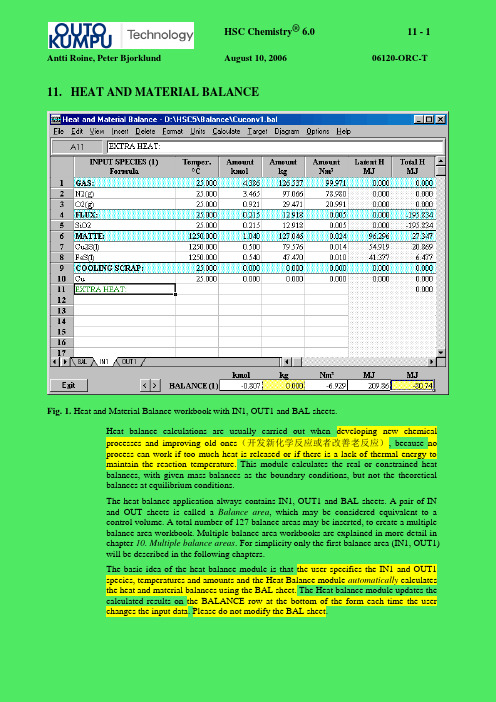
11. HEAT AND MATERIAL BALANCEFig. 1. Heat and Material Balance workbook with IN1, OUT1 and BAL sheets.Heat balance calculations are usually carried out when developing new chemicalprocesses and improving old ones(开发新化学反应或者改善老反应), because noprocess can work if too much heat is released or if there is a lack of thermal energy tomaintain the reaction temperature. This module calculates the real or constrained heatbalances, with given mass-balances as the boundary conditions, but not the theoreticalbalances at equilibrium conditions.The heat balance application always contains IN1, OUT1 and BAL sheets. A pair of INand OUT sheets is called a Balance area, which may be considered equivalent to acontrol volume. A total number of 127 balance areas may be inserted, to create a multiplebalance area workbook. Multiple balance area workbooks are explained in more detail inchapter 10. Multiple balance areas. For simplicity only the first balance area (IN1, OUT1)will be described in the following chapters.The basic idea of the heat balance module is that the user specifies the IN1 and OUT1species, temperatures and amounts and the Heat Balance module automatically calculatesthe heat and material balances using the BAL sheet. The Heat balance module updates thecalculated results on the BALANCE row at the bottom of the form each time the userchanges the input data. Please do not modify the BAL sheet.Since the program uses and creates new balance areas according to the name of the sheets,it is extremely important that the automatically created sheet names, i.e. the BAL, INxand OUTx sheets, should not be modified.You can also add new sheets for other spreadsheet calculations using the Insert Sheetand Insert Excel Sheet selections in the menu. The other sheets work very much like MSExcel worksheets, for example, you can:- rename the sheet name by double clicking the sheet tab- type formulae into the cells- use similar cell references as in Excel- use most of the Excel functions- link the sheet to IN1 sheet using normal Excel cell references, for example, for converting elemental analysis of the raw material to amounts of the components.- use the heat balance calculation results in OUT1 sheet as the initial values for other spreadsheet calculations.In addition the Heat Balance menu provides a wide range of Excel type features, such as:number, font, alignment and border formatting, defined names settings and cell protection.Because they are not necessarily needed in heat balance calculations, these features arenot described here in detail.The new heat balance module offers several ways to calculate heat and material balances:1.The user types the input and output species, temperatures and amounts into the IN1and OUT1 sheets respectively. This is a simple way to calculate heat and materialbalances and was available already in HSC 2.0. However, the problem with the oldversion was that the user had to manually maintain the material balance when theinput feed changed.2.Materials (species) are given as groups of substances, called streams. Thesestreams can be the same as the phases, but they can also be a mixture of phases.3.The output amounts can be linked with the input amounts with Excel type cellreferences, or vice versa.11.1 Basic Calculation Procedure(基本计算程序)The following procedure will describe the most simple way to calculate Heat Balance:1.Introduce the input substances (raw materials), temperatures and amounts on theIN1 sheet. It is possible to either type amounts in kmol, kg or Nm3. It is advised touse kmol and kg because missing density data may cause inaccuracy with Nm3units.2.Introduce the output substances (products), temperatures and amounts on the OUT1sheet. Type amounts in either kmol, kg or Nm3 as preferred.3.When feeding additional energy (electricity) to the process, enter this amount intothe Total column in the last empty row of the IN1 sheet. You can also type forexample “Extra Heat” in the first column of this row, see Fig. 20. The Databasemodule will convert the color of a ll “inert“ text in the first column to green, if thistext is not identified in the database as a substance. Notice that:1 kWh = 3.6 MJ = 0.8604 Mcal (th).H owever, the Balance module will automatically recalculate green text whenchanging units from the menu. If the green text cell contains a formula, it willautomatically be changed according to the new unit. For example a change from °C to K will add “+ 273.15” to the end of the formula.4.If heat loss values are known then type them into the last empty row of the OUT1sheet in the last column (Total). A first estimate of heat losses for an air-cooled reactor (natural convection) can easily be calculated using the following formula in kcal/h:Hloss = (6.8 + 0.046 * T2) * (T2 - T1) * A [1] Where: A = Outer surface area of the reactor (m2)T2= Surface temperature of the reactor (°C)T1= Room temperature (°C)P lease use the Heat Loss module if more accurate heat loss approximations are needed.5.HSC automatically and immediately updates the heat balance on the bottom line assoon as changes to any input data are made.6.HSC also automatically updates the material amount balances in mol, kg and Nm3units. Notice that only the mass balance in kg units on the bottom row should be zero; the mole or volume balances can easily change in any chemical process.7.The element balance can be checked by selecting Element Balance from theCalculate menu, see Figs. 1 and 2.8.By selecting Temperature Balance from the Calculate menu it is possible to seethe estimated temperature of the products when the heat balance = 0, see Figs. 1 and 3.Fig. 2. Element Balance.Fig. 3. Temperature of the products (adiabatic process).9.To insert an empty row in the table, select Row from the Insert menu or bypressing the right mouse button and selecting Insert Row from the popup menu.10.Rows can be deleted by selecting Row from the Delete menu or pressing the rightmouse button and selecting Del Row from the popup menu.11.You can change the order of the substances by inserting an empty row and usingthe Copy - Paste method to insert the substance in the new row. The Drag and Dropmethod can also be used. However, it is extremely important to Copy and Pastethe whole row not only the formula, because of auxiliary data in the hiddencolumns on the right side of the IN1 and OUT1 sheets.Please keep the Copy Mode selection on in the Edit menu when rearranging thespecies, as this will force the program to select the whole row. When formatting thecolumns and cells, turn the Copy Mode selection off in the Edit menu.12.Temperature units can be changed by selecting the C or K from the Units menu.13.Energy units can be changed by selecting Mcal, MJ or kWh from the Units menu.14.If a paper copy is needed, select Print from the File menu. This option will copyall the data on the same Print sheet and will also print this sheet on paper if the userpresses OK. Notice that you can delete this Print sheet by activating it and thenselecting Sheet from the Delete menu. The Print Sheet selection in the File menuwill print only the active sheet.15.To save the sheets, select Save from the File menu. Please save sheets often usingdifferent names, because you may wish to make small changes later or to return tothe original sheet. Saving sheets is important, because the Undo feature is notavailable in HSC Chemistry.16.It is possible to take into account the water/steam pressure compensation bymoving the cursor to an H2O or H2O(g) species and selecting Insert/Pressurecorrection H2O from the menu. This will open the Pressure and Temperaturecalculator, where it is possible to specify the pressure for the species. This is usefulwhen calculating for example steam processes.11.2 Formatting the WorksheetThe heat balance module offers several Excel type formatting possibilities. These may beselected in the Format menu:- Number, Font, Font Default, Alignment, Border, Pattern, Object (for graphical objects), Sheet, Options- Column Width, Row Height- Define Names, Refresh Names- Protection On, Off, Lock all Cells, Unlock all CellsThe window size may also be changed from the View menu. The Normal selection givesa VGA size window, Full Height selection uses the whole height of the screen and FullWidth fills the whole screen.11.3 Specification of Substance Groups (Streams)The new HSC Chemistry 5.0 offers the possibility to specify the input and outputsubstances in streams. These streams can be made of one or several physical phases orspecies which have the same fixed temperature and elemental composition. Although heatand material balance calculations can be made without using the streams, division intostreams helps considerably when changing temperatures and material amounts. Noticethat when using formulae/links in temperature cells the temperature cells are not updatedif the species are not divided into streams.Examples of “one-phase streams” are, for example:1.Air feed.2.Process gas output.3.Homogenous liquid and solid inputs and outputs.Examples of “multi-phase streams” are, for example:1.Liquid material with solid particles (suspension) as input or output.2.Solid feed mixture of the process, made of different substances, such as mineralconcentrate, coal and sand.3.Gas feed with liquid droplets or solid powder.The species rows in the IN1 and OUT1 sheets are divided into separate groups by specialstream rows. These rows can be inserted in the sheet using the Stream selection in theInsert menu or using the same selection in the popup menu from the right mouse button.The heat balance module automatically makes the following modifications to the sheetwhen you insert a new stream (group) row in the sheet:1.Asks for a name for the new group, which you can change later if necessary.2.Inserts a new empty row above the selected cell with a light blue pattern.3.HSC assumes that all rows under the new group row will belong to the new groupdown to the next group row.4.Inserts Excel type SUM formulae in the new group row for calculating the totalamount in the group using kmol, kg and Nm3 units.Once the insert procedure is ready, you can edit the group row in the following way:1.The stream name (label) can be edited directly in the cell.2.The stream temperature can also be changed directly in the cell and will affect thetemperature of all the species in this group.3.The total material amount of the group can be changed simply by typing a newamount in the group row in kmol, kg or Nm3units. This amount can be typeddirectly over the SUM formula and the program will automatically change theamounts of the species keeping the overall composition constant. The program willthen regenerate the original SUM formula after calculating the new amounts.4.It is important to note that you are unable to type formulae in the amount andenthalpy columns of the stream row, because the SUM formulae must be in thestream row.To change the amounts of species in a stream using kmol, kg or Nm3 units, simply typethe new amount in the corresponding cell. The program will automatically update theamounts in the other columns, total amount of the stream and the total material and heatbalance as well.An example of the species streams can be seen in Fig. 4. The output species have beendivided into four streams. In this example the species in each stream exist in the samephase. Process Gas is a gaseous mixture phase, Slag is a molten mixture phase andWhite Metal is a pure molten substance.Fig. 4. The OUT1 sheet of the Heat Balance module. The species have been divided into three streams, which are the same as the existing phases.11.4 Formulae in the CellsExcel-type formulae and cell references can be used, for example, in order to link theinput and output amounts with each other and to maintain the material balanceautomatically when the input amounts change. The input and output amounts can belinked using two main methods:1.An Excel-type formula can be typed in the kmol column, which expresses thedependence of the output mole amount on the input mole amount. For example, ifCu2S in the cell OUT1!C10 contains 93.8 % of copper input then you may typeformula = 0.938*IN1!C7 in cell OUT1!C10, see Fig 5.2.The Heat balance module automatically calculates input and output mole amountsfor elements. The cell names for input amounts are: InAc, InAg, InAl, InAm andthe equivalent for output elements are called OutAc, OutAg, OutAl, OutAm, etc.For balance areas with a higher number (for example the IN2 and OUT2 sheets) thecorresponding cell names are simply InAc2, InAc3 and OutAc2, OutAc3, etc.These names can be used in the formulae. The formula in the previous example canalso be written:=0.938*(InCu-C12)/2 using these defined names, see Fig. 5. Thecells with element amounts are not visible to the user.Please be very careful when using default input and output names simultaneously,because it is very easy to end up with circular references. An indication of acircular reference is that the heat and material balance, which can be seen on theBALANCE row, changes even after a recalculation (Calculate/ReCalc from themenu). By selecting Format/Options from the menu and highlighting theIteration checkbox under the Calculation tab, it is possible to automatically iteratethe circular references. This is, however, not recommended for very largeworksheets.Within the IN1 and OUT1 sheets it is recommended to use formulae only in the kmolcolumn and not in the other Amount columns. You can use the formulae also in othercolumns, but please be very careful. In the other sheets there are no special limitations forthe formulae.Fig. 5. The OUT1 sheet of the Heat Balance module. Copper output has been linked with copper input with a formula and defined name: InCu.11.5 Elemental CompositionsThe elemental compositions of the species groups may be calculated using the StreamCompositions selection in the Calculate menu, see Fig. 6. This procedure calculates theelemental compositions of each group, creates new In1-% and Out1-% sheets and printsresults on these new sheets in mol-% and wt-% units.Notice that a procedure to convert elemental analysis back to species analysis is not yetavailable in the heat balance module. A general solution to this kind of problem is quitedifficult and in many cases impossible. However, a custom-made solution for anindividual case is possible with a little effort and normal Excel-type formulae:1.Create a new sheet using the Sheet selection in the Insert menu, see Fig. 6.2.Rename the new sheet by double clicking the tab, for example to “Compositions”.Notice that you can use also the Input-% sheet as the starting point as you rename it.3.Type the elemental and species compositions on the new sheet.4.Notice that you can insert Formula Weights in this new sheet by selecting thechemical formula cells and then selecting Mol Weight from the Insert menu.5.Create Excel-type formulae, which convert the elemental analysis of a group tomole amounts of species using formula weights of the elements and species.6.Type formulae in the kmol columns of the IN1 sheet, which refer to speciesamounts in the Compositions sheet.Fig. 6. The Out1-% sheet of the Heat Balance module. This sheet shows the elemental compositions of the phases, after the Stream Compositions option has been selected from the Calculate menu.11.6 Additional SheetsThe Heat Balance workbook consists at least of the IN1, OUT1 and BAL sheets. The usermay, however, add up to 256 sheets to one workbook. These additional sheets may beused, for example, to convert the elemental compositions of raw materials to amounts ofspecies which are needed in the IN1 sheet. These sheets can also be used to collect themain results from the OUT1 sheet in one summary table. Do not use the reserved namesIN1, OUT1, BAL and Target as sheet names.To add sheets select Insert Sheet from the menu. This will add one sheet on the selectedlocation. To rename this new sheet, double click the Tab on the bottom of the form. Youcan also import Excel sheets by selecting Insert Excel Sheet from the menu. Thisselection allows you first to select the file and then the sheet which you want to insert intothe active Heat Balance workbook.The example in Fig. 7 shows a FEED sheet, which is used to specify the raw materialsamounts to the IN1 sheet. The user may give the compositions and amounts in column C,this data will then be used to calculate the amounts of species in column F. The materialamounts in IN1 sheet are given using relevant cell references to column F in the FEEDsheet. This example can be found from your HSC5\Balance directory under the nameCUCONV2.BAL. The user can construct the layout of the additional sheets freely.The “Red Font Shield”property is a useful way to prevent accidental modification of thedata in the cells. If this property is set using menu selection Format, Red Font Shieldthen only cells with red font can be edited. However, it is recommended to save the workregularly using different names, for example, test1.bal, test2.bal, test3.bal, etc. in order torecover the original situation after harmful modifications.Fig. 7. Additional sheets can be added to the Heat Balance workbook.11.7 Target DialogThe user can iterate manually, for example, the fuel amount which is needed to achievezero heat balance by changing the fuel amount until the heat balance is zero. The Targetsheet offers a faster automatic way to carry out these kind of iterations. The followinginstructions will explain this procedure in more detail:1.Select Target Dialog from the menu. This will also automatically create a Targetsheet, which is similar to previous HSC versions.2.Select one cell on row 4 in the Target dialog if not selected.3.Select one cell which will be used as a first variable and select Set variable cell.This will add the cell reference of this variable to the Target dialog in column B.You can also type the cell references manually in the Target dialog. Note: Pleaseuse only Stream temperature cells as variables for the temperature iterations, ie. donot use species temperature cells.4.Select one cell which will be used as first variable and select Set target cell. Thiswill add the cell reference of this variable to the Target dialog in column B.5.Repeat steps 3 and 4 if you want to add more variables and targets.6.Set valid Min and Max limits in columns D and E as well as the Target Value incolumn H. You may also type names in columns A and F.ually it is also necessary to give estimated initial Test Values in column C forthe automatic iterations. Iteration ends when the target value (col H) or iterationnumber (col I) is reached. Accuracy can be improved by increasing the number ofdecimals used in columns G and H with the Format Number selection.8.Select the rows (> 3) on the Target sheet which you want to iterate and pressIterate selected rows or F8. If all rows should be iterated, simply press Iterate All.In the following example, shown in Fig. 8, you can select for example row 4 and press F8.This will evaluate the copper scrap amount which is needed to maintain the heat balancein the given conditions. Row 5 can be used to iterate the iron content of the matte in thesame conditions and row 6 to achieve a given FeS amount.Important note: Please use only Stream temperature cells as variables for the temperatureiterations, ie. do not use species temperature cells.Fig. 8. Target dialog specifies the variables and target cell references.11.8 GraphicsOccasionally it is useful to see the results, of for example a heat balance calculation, ingraphical format. This can be carried out manually by making step by step changes to onevariable cell and collecting data from interesting cells, for example, to an Excel sheet.Sometimes further calculations may be required after every step, which can be specifiedusing the Diagram Dialog. Step by step the procedure is as follows:1.Select Diagram/Diagram Dialog from the menu.2.Select the variable cell and press Set X-cell from the dialog. Select, for example,cell C11, see Fig. 7.3.Select a cell for the y-axis and press Set Y-cell from the dialog. Select, for example,the Heat Balance cell at the bottom right of the form. You may repeat this step andcollect several cells whose values will be drawn to the diagram.4.If other calculations are required between every step, press Target iteration andthe Target sheet will automatically open. Select the calculation rows that should beiterated before the Y-row and press Set Target rows from the menu. The row datawill now be tranferred to the Diagram dialog into columns 4, 5, etc.5.Fill the Diagram Settings as shown in Fig. 9. You must specify the MIN, MAX andSTEP values for the X-Axis. You can also specify the cell references, labels andunits manually in this form.6.Press Diagram to create the tabular data for the diagram and Diagram once againto see the final diagram, Fig 9.7.The diagram can be modified, copied and printed in the same manner as otherdiagrams in HSC Chemistry.8.Show/Toolbar shows the drawing menu and Show/Object Editor shows theobject editor, which lets you specify the objects manually.9.To return to the Heat Balance module, press Exit at the bottom left corner of thediagram form.From the diagram shown in Fig. 9 you can see that roughly 68 kg/h of scrap is needed toadjust the heat balance to zero. Notice that the units in the diagram are kg/h and kW.Fig. 9. Simple heat balance diagram.In the following diagram (Fig. 10) the heat balance is automatically calculated beforeeach step, which is indicated by the number “4” in the Target row 1 column. This is doneby pressing the Target iteration button, selecting row 4 on the Target sheet and clickingthe Set Target rows button. The x-axis now gives the Fe wt-% and the y-axis the coolingscrap required. The diagram may then be interpreted as the quantity of cooling scraprequired to make the heat balance zero, when the Fe wt-% varies from 20% to 25%.Fig. 10. Diagram where the heat balance is automatically iterated to zero before every calculation step.11.9 Multiple balance areas(多个物料平衡)The previous Balance modules up to HSC 4.0 were restricted to one balance area (orcontrol volume) only. Since most processes consist of multiple balance areas, the newBalance module enables the user to create up to 127 multiple balance areas. A balancearea consists of an INx and an OUTx sheet, where x denotes the number of the balancearea. These can then be connected to each other creating a realistic simulation of aprocess. The example file FSF_process.BAL contains a highly simplified multibalancemodel of an Outokumpu Flash Smelting Furnace process.A new balance area is created by selecting either Insert/Balance Area to Right orInsert/Balance Area to Left from the menu. This will insert a pair of INx and OUTxsheets to the corresponding position. A balance area may easily be deleted by selectingDelete/Balance Area. Deleting a single sheet of a balance area, for example an INx sheet,is not possible. The balances are all automatically collected into the BAL sheet so pleasedo not modify this sheet.Fig. 11. The BAL sheet when the worksheet consists of 5 balance areas.Linking the balance areas with each other is recommended to carry out after eachindividual balance areas operate properly. Linking may be achieved either manuallywith formulae or automatically with the Copy - Paste Stream combination. Simply placethe cursor on a stream row in an OUTx sheet, or on a row that belongs to a stream, andselect Edit/Copy. Then place the cursor on a row in an INx sheet and select Edit/PasteStream. The stream will now be copied here so that the first row of the stream is the cursor position. The kmol column of the pasted stream will consist of links (formulae) to the copied stream, so that the material amounts of the streams will remain equal. The other cells are directly copied as values. If the stream temperature cell in the copied stream is a formulae then it will not be copied. In this case it is up to the user to decide how the stream temperature for the pasted stream should be calculated.It is also possible to create return streams, i.e. streams that return to a previous part of the process, thus creating loops in the process. When pasting a stream into an already linked part, a circular reference might occur. This is the case when links eventually refer back to each other, i.e. iterations are needed to calculate the worksheet. Automatic iterations may be done by selecting Format/Options from the menu and highlighting the Iteration checkbox under the Calculation tab. Please be careful when changing the inputs of a worksheet consisting of circular references. For example if a cell, which is part of a circular reference, shows the message #VALUE!, it will not recover unless the links in the cells are changed thus breaking the circular reference. Saving the worksheet regularly using different names (Test1, Test2, etc.) is thus always recommended.Fig. 12. The IN1 sheet (Flash Furnace) of the FSF_process.BAL example. The stream Flue dust is a return stream from the boiler (Copy/Paste stream), thus creating circular references in the worksheet.Automatically updated defined names (input and output kmol amounts) vary according to thebalance area. For example InAl, InC, OutFe for the first balance area will become InAl2, InC2,OutFe2 for the second etc. Note that the defined names of the first balance area do not haveindex numbers.Fig. 13. The OUT2 sheet (Converter I), gives the output from the first part of the converter. The formula =InCa2*Analysis!L29/100 in cell C5 means that the total Ca is distributed as the percentage given in cell L29 on the Analysis sheet.Drawing Flowsheets (Flowcharts)Additional sheets may be used to collect, for example, all the necessary input for the processinto one sheet. They may also be used to collect calculated process parameters, for examplethe amount of Cu in a stream. Figure 14 shows the process layout for the Flash SmeltingFurnace process."Insert, Graphical Object, ..." selection gives possibility to draw lines, rectangles, etc. on theadditional sheets. However, it is recommended to draw flowsheets using "Format, Border, ..."and "Format, Pattern, ..." selection because these properties are more compatible with Excel95, 97 and 2000. Arrows may be drawn using "Insert, Graphical Object, Arrow" selection.HSC graphical objects are compatible only with Excel 95. This means that if you want to getthe graphical objects to Excel-files then you should save using "File, Save XLS 5 file, ..."dialog.Fig. 14. Process layout and input sheet for the Flash Smelting Furnace process.。
Fluent用户手册
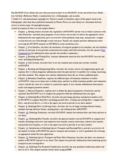
The FLUENT User's Guide tells you what you need to know to use FLUENT. At the end of the User's Guide, you will find a Reference Guide, a nomenclature list, a bibliography, and an index.!! Under U.S. and international copyright law, Fluent is unable to distribute copies of the papers listed in the bibliography, other than those published internally by Fluent. Please use your library or a document delivery service to obtain copies of copyrighted papers.A brief description of what's in each chapter follows:•Chapter 1, Getting Started, describes the capabilities of FLUENT and the way in which it interacts with other Fluent Inc. and third-party programs. It also advises you on how to choose the appropriate solverformulation for your application, gives an overview of the problem setup steps, and presents a samplesession that you can work through at your own pace. Finally, this chapter provides information aboutaccessing the FLUENT manuals on CD-ROM or in the installation area.•Chapter 2, User Interface, describes the mechanics of using the graphical user interface, the text interface, and the on-line help. It also provides instructions for remote and batch execution. (See the separate Text Command List for information about specific text interface commands.)•Chapter 3, Reading and Writing Files, contains information about the files that FLUENT can read and write, including hardcopy files.•Chapter 4, Unit Systems, describes how to use the standard and custom unit systems available in FLUENT.•Chapter 5, Reading and Manipulating Grids, describes the various sources of computational grids and explains how to obtain diagnostic information about the grid and how to modify it by scaling, translating, and other methods. This chapter also contains information about the use of non-conformal grids.•Chapter 6, Boundary Conditions, explains the different types of boundary conditions available in FLUENT, when to use them, how to define them, and how to define boundary profiles and volumetric sources and fix the value of a variable in a particular region. It also contains information about porousmedia and lumped parameter models.•Chapter 7, Physical Properties, explains how to define the physical properties of materials and the equations that FLUENT uses to compute the properties from the information that you input.•Chapter 8, Modeling Basic Fluid Flow, describes the governing equations and physical models used by FLUENT to compute fluid flow (including periodic flow, swirling and rotating flows, compressibleflows, and inviscid flows), as well as the inputs you need to provide to use these models.•Chapter 9, Modeling Flows in Moving Zones, describes the use of single rotating reference frames, multiple moving reference frames, mixing planes, and sliding meshes in FLUENT.•Chapter 10, Modeling Turbulence, describes FLUENT's models for turbulent flow and when and how to use them.•Chapter 11, Modeling Heat Transfer, describes the physical models used by FLUENT to compute heat transfer (including convective and conductive heat transfer, natural convection, radiative heat transfer,and periodic heat transfer), as well as the inputs you need to provide to use these models.•Chapter 12, Introduction to Modeling Species Transport and Reacting Flows, provides an overview of the models available in FLUENT for species transport and reactions, as well as guidelines for selectingan appropriate model for your application.•Chapter 13, Modeling Species Transport and Finite-Rate Chemistry, describes the finite-rate chemistry models in FLUENT and how to use them. This chapter also provides information about modeling species transport in non-reacting flows.•Chapter 14, Modeling Non-Premixed Combustion, describes the non-premixed combustion model and how to use it. This chapter includes details about using prePDF.•Chapter 15, Modeling Premixed Combustion, describes the premixed combustion model and how to use it.•Chapter 16, Modeling Partially Premixed Combustion, describes the partially premixed combustion model and how to use it.•Chapter 17, Modeling Pollutant Formation, describes the models for the formation of NOx and soot and how to use them.•Chapter 18, Introduction to Modeling Multiphase Flows, provides an overview of the models for multiphase flow (including the discrete phase, VOF, mixture, and Eulerian models), as well as guidelines for selecting an appropriate model for your application.•Chapter 19, Discrete Phase Models, describes the discrete phase models available in FLUENT and how to use them.•Chapter 20, General Multiphase Models, describes the general multiphase models available in FLUENT (VOF, mixture, and Eulerian) and how to use them.•Chapter 21, Modeling Solidification and Melting, describes FLUENT's model for solidification and melting and how to use it.•Chapter 22, Using the Solver, describes the FLUENT solvers and how to use them.•Chapter 23, Grid Adaption, explains the solution-adaptive mesh refinement feature in FLUENT and how to use it.•Chapter 24, Creating Surfaces for Displaying and Reporting Data, explains how to create surfaces in the domain on which you can examine FLUENT solution data.•Chapter 25, Graphics and Visualization, describes the graphics tools that you can use to examine your FLUENT solution.•Chapter 26, Alphanumeric Reporting, describes how to obtain reports of fluxes, forces, surface integrals, and other solution data.•Chapter 27, Field Function Definitions, defines the flow variables that appear in the variable selection drop-down lists in FLUENT panels, and tells you how to create your own custom field functions. •Chapter 28, Parallel Processing, explains the parallel processing features in FLUENT and how to use them. This chapter also provides information about partitioning your grid for parallel processing.18. Introduction to Modeling Multiphase FlowsA large number of flows encountered in nature and technology are a mixture of phases. Physical phases of matter are gas, liquid, and solid, but the concept of phase in a multiphase flow system is applied in a broader sense. In multiphase flow, a phase can be defined as an identifiable class of material that has a particular inertial response to and interaction with the flow and the potential field in which it is immersed. For example, different-sized solid particles of the same material can be treated as different phases because each collection of particles with the same size will have a similar dynamical response to the flow field.This chapter provides an overview of multiphase modeling in FLUENT, and Chapters 19 and 20 provide details about the multiphase models mentioned here. Chapter 21 provides information about melting and solidification.18.1 Multiphase Flow RegimesMultiphase flow can be classified by the following regimes, grouped into four categories:gas-liquid or liquid-liquid flowsbubbly flow: discrete gaseous or fluid bubbles in a continuous fluiddroplet flow: discrete fluid droplets in a continuous gasslug flow: large bubbles in a continuous fluidstratified/free-surface flow: immiscible fluids separated by a clearly-defined interfacegas-solid flowsparticle-laden flow: discrete solid particles in a continuous gaspneumatic transport: flow pattern depends on factors such as solid loading, Reynolds numbers, and particle properties. Typical patterns are dune flow, slug flow, packed beds, and homogeneous flow.fluidized beds: consist of a vertical cylinder containing particles where gas is introduced through a distributor. The gas rising through the bed suspends the particles. Depending on the gas flow rate, bubbles appear and rise through the bed, intensifying the mixing within the bed.liquid-solid flowsslurry flow: transport of particles in liquids. The fundamental behavior of liquid-solid flows varies with the properties of the solid particles relative to those of the liquid. In slurry flows, the Stokes number (seeEquation 18.4-4) is normally less than 1. When the Stokes number is larger than 1, the characteristic of the flow is liquid-solid fluidization.hydrotransport: densely-distributed solid particles in a continuous liquidsedimentation: a tall column initially containing a uniform dispersed mixture of particles. At the bottom, the particles will slow down and form a sludge layer. At the top, a clear interface will appear, and in the middle a constant settling zone will exist.three-phase flows (combinations of the others listed above)Each of these flow regimes is illustrated in Figure 18.1.1.Figure 18.1.1: Multiphase Flow Regimes18.2 Examples of Multiphase SystemsSpecific examples of each regime described in Section 18.1 are listed below:Bubbly flow examples: absorbers, aeration, air lift pumps, cavitation, evaporators, flotation, scrubbersDroplet flow examples: absorbers, atomizers, combustors, cryogenic pumping, dryers, evaporation, gas cooling, scrubbersSlug flow examples: large bubble motion in pipes or tanksStratified/free-surface flow examples: sloshing in offshore separator devices, boiling and condensation in nuclear reactorsParticle-laden flow examples: cyclone separators, air classifiers, dust collectors, and dust-laden environmental flowsPneumatic transport examples: transport of cement, grains, and metal powdersFluidized bed examples: fluidized bed reactors, circulating fluidized bedsSlurry flow examples: slurry transport, mineral processingHydrotransport examples: mineral processing, biomedical and physiochemical fluid systemsSedimentation examples: mineral processing18.3 Approaches to Multiphase ModelingAdvances in computational fluid mechanics have provided the basis for further insight into the dynamics of multiphase flows. Currently there are two approaches for the numerical calculation of multiphase flows: the Euler-Lagrange approach and the Euler-Euler approach.18.3.1 The Euler-Lagrange ApproachThe Lagrangian discrete phase model in FLUENT (described in Chapter 19) follows the Euler-Lagrange approach. The fluid phase is treated as a continuum by solving the time-averaged Navier-Stokes equations, while the dispersed phase is solved by tracking a large number of particles, bubbles, or droplets through the calculated flow field. The dispersed phase can exchange momentum, mass, and energy with the fluid phase.A fundamental assumption made in this model is that the dispersed second phase occupies a low volume fraction, even though high mass loading ( ) is acceptable. The particle or droplet trajectories are computed individually at specified intervals during the fluid phase calculation. This makes the model appropriate for the modeling of spray dryers, coal and liquid fuel combustion, and some particle-laden flows, but inappropriate for the modeling of liquid-liquid mixtures, fluidized beds, or any application where the volume fraction of the second phase is not negligible.18.3.2 The Euler-Euler ApproachIn the Euler-Euler approach, the different phases are treated mathematically as interpenetrating continua. Since the volume of a phase cannot be occupied by the other phases, the concept of phasic volume fraction is introduced. These volume fractions are assumed to be continuous functions of space and time and their sum is equal to one. Conservation equations for each phase are derived to obtain a set of equations, which have similar structure for all phases. These equations are closed by providing constitutive relations that are obtained from empirical information, or, in the case of granular flows , by application of kinetic theory.In FLUENT, three different Euler-Euler multiphase models are available: the volume of fluid (VOF) model, the mixture model, and the Eulerian model.The VOF ModelThe VOF model (described in Section 20.2) is a surface-tracking technique applied to a fixed Eulerian mesh. It is designed for two or more immiscible fluids where the position of the interface between the fluids is of interest. In the VOF model, a single set of momentum equations is shared by the fluids, and the volume fraction of each of the fluids in each computational cell is tracked throughout the domain. Applications of the VOF model include stratified flows , free-surface flows, filling, sloshing , the motion of large bubbles in a liquid, the motion of liquid after a dam break, the prediction of jet breakup (surface tension), and the steady or transient tracking of any liquid-gas interface.The Mixture ModelThe mixture model (described in Section 20.3) is designed for two or more phases (fluid or particulate). As in the Eulerian model, the phases are treated as interpenetrating continua. The mixture model solves for the mixture momentum equation and prescribes relative velocities to describe the dispersed phases. Applications of the mixture model include particle-laden flows with low loading, bubbly flows, sedimentation , and cyclone separators. The mixture model can also be used without relative velocities for the dispersed phases to model homogeneous multiphase flow.The Eulerian ModelThe Eulerian model (described in Section 20.4) is the most complex of the multiphase models in FLUENT. It solves a set of n momentum and continuity equations for each phase. Coupling is achieved through the pressure and interphase exchange coefficients. The manner in which this coupling is handled depends upon the type of phases involved; granular (fluid-solid) flows are handled differently than non-granular (fluid-fluid) flows. For granular flows , the properties are obtained from application of kinetic theory. Momentum exchange between the phases is also dependent upon the type of mixture being modeled. FLUENT's user-defined functions allow you tocustomize the calculation of the momentum exchange. Applications of the Eulerian multiphase model include bubble columns , risers , particle suspension, and fluidized beds .18.4 Choosing a Multiphase ModelThe first step in solving any multiphase problem is to determine which of the regimes described inSection 18.1 best represents your flow. Section 18.4.1 provides some broad guidelines for determining appropriate models for each regime, and Section 18.4.2 provides details about how to determine the degree of interphase coupling for flows involving bubbles, droplets, or particles, and the appropriate model for different amounts of coupling.18.4.1 General GuidelinesIn general, once you have determined the flow regime that best represents your multiphase system, you can select the appropriate model based on the following guidelines. Additional details and guidelines for selecting the appropriate model for flows involving bubbles, droplets, or particles can be found in Section 18.4.2.For bubbly, droplet, and particle-laden flows in which the dispersed-phase volume fractions are less than or equal to 10%, use the discrete phase model. See Chapter 19 for more information about the discrete phase model.For bubbly, droplet, and particle-laden flows in which the phases mix and/or dispersed-phase volume fractions exceed 10%, use either the mixture model (described in Section 20.3) or the Eulerian model (described in Section 20.4). See Sections 18.4.2 and 20.1 for details about how to determine which is more appropriate for your case.For slug flows, use the VOF model. See Section 20.2 for more information about the VOF model.For stratified/free-surface flows, use the VOF model. See Section 20.2 for more information about the VOF model.For pneumatic transport, use the mixture model for homogeneous flow (described in Section 20.3) or the Eulerian model for granular flow (described in Section 20.4). See Sections 18.4.2 and 20.1 for details about how to determine which is more appropriate for your case.For fluidized beds, use the Eulerian model for granular flow. See Section 20.4 for more information about the Eulerian model.For slurry flows and hydrotransport , use the mixture or Eulerian model (described, respectively, inSections 20.3 and 20.4). See Sections 18.4.2 and 20.1 for details about how to determine which is more appropriate for your case.For sedimentation, use the Eulerian model. See Section 20.4 for more information about the Eulerian model.For general, complex multiphase flows that involve multiple flow regimes, select the aspect of the flow that is of most interest, and choose the model that is most appropriate for that aspect of the flow. Note that the accuracy of results will not be as good as for flows that involve just one flow regime, since the model you use will be valid for only part of the flow you are modeling.18.4.2 Detailed GuidelinesFor stratified and slug flows, the choice of the VOF model, as indicated in Section 18.4.1, is straightforward. Choosing a model for the other types of flows is less straightforward. As a general guide, there are some parameters that help to identify the appropriate multiphase model for these other flows: the particulate loading, , and the Stokes number, St. (Note that the word ``particle'' is used in this discussion to refer to a particle, droplet, or bubble.)The Effect of Particulate LoadingParticulate loading has a major impact on phase interactions. The particulate loading is defined as the mass density ratio of the dispersed phase ( d) to that of the carrier phase ( c):The material density ratiois greater than 1000 for gas-solid flows, about 1 for liquid-solid flows, and less than 0.001 for gas-liquid flows. Using these parameters it is possible to estimate the average distance between the individual particles of the particulate phase. An estimate of this distance has been given by Crowe et al. [ 42]:where . Information about these parameters is important for determining how the dispersed phase shouldbe treated. For example, for a gas-particle flow with aparticulate loading of 1, the interparticle space is about 8; the particle can therefore be treated as isolated (i.e., very low particulate loading).Depending on the particulate loading, the degree of interaction between the phases can be divided into three categories:For very low loading, the coupling between the phases is one-way; i.e., the fluid carrier influences the particles via drag and turbulence, but the particles have no influence on the fluid carrier. The discrete phase, mixture, and Eulerian models can all handle this type of problem correctly. Since the Eulerian model is the most expensive, the discrete phase or mixture model is recommended.For intermediate loading, the coupling is two-way; i.e., the fluid carrier influences the particulate phase via drag and turbulence, but the particles in turn influence the carrier fluid via reduction in mean momentum and turbulence. The discrete phase, mixture, and Eulerian models are all applicable in this case, but you need to take into account other factors in order to decide which model is more appropriate. See below for information about using the Stokes number as a guide.For high loading, there is two-way coupling plus particle pressure and viscous stresses due to particles (four-way coupling). Only the Eulerian model will handle this type of problem correctly.The Significance of the Stokes NumberFor systems with intermediate particulate loading, estimating the value of the Stokes number can help you select the most appropriate model. The Stokes number can be defined as the relation between the particle response time and the system response time:where and t s is based on the characteristic length ( L s) and the characteristic velocity ( V s) of the system under investigation: .For , the particle will follow the flow closely and any of the three models (discrete phase, mixture, or Eulerian) is applicable; you can therefore choose the least expensive (the mixture model, in most cases), or themost appropriate considering other factors. For , the particles will move independently of the flowand either the discrete phase model or the Eulerian model is applicable. For , again any of the three models is applicable; you can choose the least expensive or the most appropriate considering other factors. ExamplesFor a coal classifier with a characteristic length of 1 m and a characteristic velocity of 10 m/s, the Stokes number is 0.04 for particles with a diameter of 30 microns, but 4.0 for particles with a diameter of 300 microns. Clearly the mixture model will not be applicable to the latter case.For the case of mineral processing, in a system with a characteristic length of 0.2 m and a characteristic velocity of 2 m/s, the Stokes number is 0.005 for particles with a diameter of 300 microns. In this case, you can choose between the mixture and Eulerian models. (The volume fractions are too high for the discrete phase model, as noted below.)Other ConsiderationsKeep in mind that the use of the discrete phase model is limited to low volume fractions. Also, the discrete phase model is the only multiphase model that allows you to specify the particle distribution or include combustion modeling in your simulation.。
ANSYS中各种错误提示解决方案

THIS ANSYS SOFTWARE PRODUCT AND PROGRAM DOCUMENTATION INCLUDE TRADE SECRETS AND ARE CONFIDENTIAL AND PROPRIETARY PRODUCTS OF ANSYS, INC., ITS SUBSIDIARIES, OR LICENSORS. The software products and documentation are furnished by ANSYS, Inc., its subsidiaries, or affiliates under a software license agreement that contains provisions concerning non-disclosure, copying, length and nature of use, compliance with exporting laws, warranties, disclaimers, limitations of liability, and remedies, and other provisions. The software products and documentation may be used, disclosed, transferred, or copied only in accordance with the terms and conditions of that software license agreement.
Copyright and Trademark Information
© 2005 SAS IP, Inc. All rights reserved. Unauthorized use, distribution or duplication is prohibited.
读书报告字体格式
附件a:读书报告书写标准一、读书报告包括题目(含关键词)、前言、文献回顾、结论、参考文献五部分。
二、具体要求1.题目力求简明、醒目,反映出文章的主题。
中文文题以不超过15个汉字为宜。
2.作者科室、姓名在文题下。
3.所有文章须标引2~5个关键词。
4.医学名词以人民卫生出版社编写的教材为准,药物名称不用商品名。
5.图表每幅图、表应有简明的题目。
要合理安排表的纵、横标目,并将数据的含义表达清楚;表内数据同一指标保留的小数位数相同。
6.计量单位按国务院1984年2月颁布的《中华人民共和国法定计量单位》书写,并以单位符号表示,例如kg。
7.缩略语首次出现处先叙述其中文全称,然后括号注出中文缩略语或英文全称及其缩略语。
8.参考文献按gb/t 7714-2005 《文后参考文献著录规则》采用顺序编码制著录,依照其在文中出现的先后顺序用阿拉伯数字加方括号标出。
参考文献的数量一般不少于10篇。
9.标题层次采用阿拉伯数字连续编码,标题层次划分一般不超过4级。
第一级标题为1,第二级标题为1.1,第三级标题为1.1.1,第四级标题为1.1.1.1。
10.题目字体要求宋体小二号,作者、关键词及正文部分均要求宋体小四号,西文字体要求times new roman。
总字数以2500~3000字为宜。
附件b:读书报告ppt制作要求1、ppt报告的内容应与读书报告原文内容一致,按照题目与关键词、前言、文献查证、结论、参考文献五个部分的内容进行汇报。
2、ppt中需标注出对应的参考文献(如下图所示),且序号与读书报告中的参考文献一致。
3、可以在ppt中适当添加相关的图片、图表或超链接内容。
4、报告内容重点突出。
附件c:读书报告评价标准姓名:???? 科室:???? 工号:????入院时间:?????? 题目:?????????????????????附件4 寻找“最美护士”摄影比赛方案值2014年“国际护士节”来临之际,医院决定在全院范围内寻找我院最美护士、捕捉护士最美瞬间摄影比赛,旨在倡导、弘扬我院护理人员甘于奉献、救死扶伤、勇于献身的人道主义精神,具体活动方案如下:一、参选方式:科室推荐、同事推荐、个人自荐。
CFX12_09_Turbulence
9-3
April 28, 2009 Inventory #002598
Turbulence
Observation by O. Reynolds
Training Manual
Laminar
(Low Reynolds Number)
Transition
(Increasing Reynolds Number)
Training Manual
Small structures
Large structures
Energy Cascade Richardson (1922)
ANSYS, Inc. Proprietary © 2009 ANSYS, Inc. All rights reserved.
9-5
April 28, 2009 Inventory #002598
Natural Convection 2 3 Ra β g L3 ∆T ρ C p β g L ∆T 9 ≥ 10 = where Ra = is the Rayleigh number Pr µk να ν µCp Pr = = is the Prandtl number α k
ANSYS, Inc. Proprietary © 2009 ANSYS, Inc. All rights reserved.
– This is the most widely used approach for calculating industrial flows
• There is not yet a single, practical turbulence model that can reliably predict all turbulent flows with sufficient accuracy
传热学英文版Chap7

For forced convection we know that Nu = f(Re, Pr). From the definition of Gr, we have Re = f(Gr); Thus for forced convection there is always:
Nu = f (Gr, Pr)
Nu f = C (Gr f Pr f ) m
m C m
More complicated relations have been provided by Churchill and Chu: 0.670 Ra 1/ 4 9 Nu f = 0.68 + for Ra < 10 L 9 / 16 4 / 9 1 + (0.492 / Pr)
The first term on the right side is the buoyancy force; introduce the volume coefficient of expansion (体积膨胀 系数) β: 1 ∂V
β=
V ∂T p
1 V − V∞ V / V∞ − 1 = V∞ T − T∞ T − T∞
Nu f = C (Gr f Pr f ) m
Ra = GrPr is called the Rayleigh number. The subscript f means the properties are evaluated at the film temperature: 1
Tf = 2 (T∞ + Tw )
u ∂x +v ∂y = −g −
Outside the boundary layer there is: u = v = 0, which yields:
海底两万里第一到十一章的景观

海底两万里第一到十一章的景观英文回答:Chapter 1: A Shifting Seascape.In the first chapter of "Twenty Thousand Leagues Under the Sea," the narrative begins with a vivid description of the ocean's ever-changing landscape. As Captain Nemo and Professor Aronnax sail aboard the Nautilus, they encounter a mesmerizing array of marine life and underwater scenery. The waters teem with colorful coral reefs, swaying gently in the current. Schools of vibrant tropical fish dart in and out of the corals, creating a dazzling display of colors. The sunlight filters through the water, casting an ethereal glow on the scene. The sea floor is covered in a carpet of soft, golden sand, interspersed with small rocks and seashells. As the Nautilus glides through the water, the landscape shifts, revealing new wonders at every turn.Chapter 2: The Lost Continent of Atlantis.In the second chapter, Captain Nemo takes the crew on a journey to the fabled lost city of Atlantis. As they descend deeper into the depths, the underwater landscape transforms into a mystical realm. They discover ancient ruins, towering pillars, and grand archways, all submerged beneath the sea. The remains of once-great buildings and structures evoke a sense of awe and wonder. The water around Atlantis is teeming with marine life, including majestic sea turtles, graceful manta rays, and curious dolphins. The city itself is adorned with intricate carvings and statues, preserved through the ages. The crew explores the streets of Atlantis, marveling at the advanced civilization that once thrived there.Chapter 3: The Enchanted Forest.Chapter 3 takes us to an enchanting underwater forest, where the Nautilus glides through a dense thicket of seaweed and kelp. The forest is alive with movement as schools of fish dart in and out of the foliage. The kelp sways gently in the current, creating a mesmerizing dance.Sunlight filters through the canopy, casting dappled patterns on the sea floor. The forest is home to a variety of creatures, including playful seals, elusive octopuses, and camouflaged seahorses. The crew of the Nautilus is captivated by the ethereal beauty of the enchanted forest, feeling as if they have stepped into a magical realm.Chapter 4: The Abyssal Plains.In the fourth chapter, the Nautilus descends into the abyssal plains, the deepest parts of the ocean. Here, the landscape is stark and desolate, characterized by vast expanses of sandy plains. The crew observes strange and otherworldly creatures, adapted to survive in the extreme conditions of the deep sea. They encounter bioluminescent organisms that illuminate the darkness with their ethereal glow. The abyssal plains are also home to unique geological formations, such as underwater mountains and deep trenches. The crew is both fascinated and humbled by the immense depths and the mysteries that lie within.Chapter 5: The Coral Kingdom.Chapter 5 transports us to a breathtaking coral kingdom, where the Nautilus navigates through a labyrinth of coral formations. The coral reefs are a riot of colors, with vibrant corals in shades of red, orange, and purple. The reefs are bustling with life, with schools of fish, sea turtles, and even sharks swimming among the corals. Thecrew explores the nooks and crannies of the reef, discovering hidden caves and crevices. They witness the delicate balance of life within the coral ecosystem, astiny fish seek shelter among the branches of the corals.The coral kingdom is a testament to the beauty anddiversity of the underwater world.Chapter 6: The Submarine Volcano.In the sixth chapter, the Nautilus ventures near a submarine volcano, where molten lava erupts from the ocean floor. The crew witnesses the raw power of nature as fiery lava spews into the water, creating billowing clouds of steam. The heat is intense, and the sea boils with energy. Despite the danger, the crew marvels at the spectacle,feeling a mix of fear and exhilaration. The volcano's surroundings are teeming with unique organisms, adapted to survive in such extreme conditions. The crew witnesses the resilience of life, even in the face of such destructive forces.Chapter 7: The Underwater Gardens.Chapter 7 takes us to the underwater gardens, where the Nautilus glides through a mesmerizing display of aquatic plants. The gardens are a riot of colors, with an abundance of seaweed, sea grass, and floating algae. The crewobserves the delicate dance of the plants as they sway in the current. The gardens are home to a variety of creatures, including sea turtles, crabs, and colorful nudibranchs. The crew is enchanted by the tranquility and beauty of the underwater gardens, feeling as if they have entered ahidden paradise.Chapter 8: The Ice Realm.In the eighth chapter, the Nautilus ventures into theicy waters of the polar regions. The landscape is dominated by vast expanses of ice, stretching as far as the eye can see. The crew witnesses the beauty of icebergs, towering structures of frozen water that glisten in the sunlight. They encounter polar bears, seals, and penguins, adapted to survive in the harsh conditions. The crew experiences the biting cold and the eerie silence of the ice realm, feeling a sense of isolation and awe.Chapter 9: The Sunken Shipwreck.Chapter 9 takes us to a sunken shipwreck, where the Nautilus explores the remains of a once-mighty vessel. The wreck is covered in a layer of silt and debris, and the crew navigates through the dark corridors and cabins. They discover artifacts and treasures, frozen in time. The wreck is also home to a variety of marine life, including curious fish and eels. The crew reflects on the fragility of human endeavors, as they witness the ship's slow decay and the relentless power of the ocean.Chapter 10: The Bioluminescent Caverns.In the tenth chapter, the Nautilus enters a network of bioluminescent caverns, where the walls and ceilings are adorned with millions of glowing organisms. The caverns are a spectacle of light, as the crew is surrounded by a mesmerizing display of colors. The bioluminescent organisms create a magical ambiance, casting an ethereal glow on the surroundings. The crew is captivated by the beauty and mystery of the caverns, feeling as if they have steppedinto a different world.Chapter 11: The Luminous Lagoon.Chapter 11 transports us to a luminous lagoon, where the Nautilus sails through waters that glow with an otherworldly light. The lagoon is alive with bioluminescent organisms, creating a spectacle of shimmering blue and green lights. The crew is dazzled by the luminosity,feeling as if they are floating among the stars. The lagoon is home to a variety of creatures, including jellyfish and plankton. The crew is enchanted by the ethereal beauty of the luminous lagoon, feeling a sense of wonder andtranquility.中文回答:第一章,变幻的海底景观。
传热学专业英语词汇
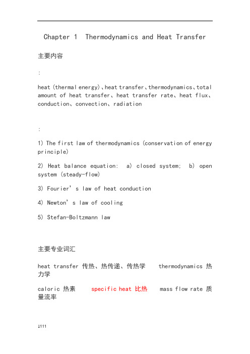
Chapter 1 Thermodynamics and Heat Transfer主要内容:heat (thermal energy)、heat transfer、thermodynamics、total amount of heat transfer、heat transfer rate、heat flux、conduction、convection、radiation:1) The first law of thermodynamics (conservation of energy principle)2) Heat balance equation: a) closed system; b) open system (steady-flow)3) Fourier’s law of heat conduction4) Newton’s law of cooling5) Stefan-Boltzmann law主要专业词汇heat transfer 传热、热传递、传热学 thermodynamics热力学caloric 热素specific heat 比热 mass flow rate 质量流率latent heat 潜热 sensible heat 显热 heat flux 热流密度heat transfer rate热流量total amount of heat transfer 总热量conduction导热 convection对流 radiation 辐射thermal conductivity 热导率 thermal diffusivity 热扩散率convection/combined heat transfer coefficient 对流/综合换热系数emissivity 发射率 absorptivity 吸收率simultaneous heat transfer 复合换热Chapter 2 Heat Conduction Equation主要内容:temperature field、temperature gradient、heat generation、initial condition、boundary condition、steady\transient heat transfer、uniform\nonuniform temperature distribution:1) Fourier’s law of heat conduction (§2-1)v1.0 可编辑可修改2) Heat conduction equation (inrectangular\cylindrical\spherical coordinates) (§2-2、§2-3)3) Boundary conditions: (§2-4)a)Specified temperature B. C.b) Specified heat flux B. C. [special case(dt/dx=0):insulation、thermal symmetry];c) Convection .d) Radiation .e) Interface .4) Average thermal conductivity k ave (§2-7)5) Solution of one-dimensional, steady heat conduction inplane walls、cylinders and spheres (k =const):a) no heat generation, specified .: T(x) or T(r) (§2-5)Q(x) or Q(r), Q=constb) with heat generation, Specified . or Convection . :(§2-6)∆T max=T o-T s= gs2/2nk ; q(x)=gx/n; T s=T+gs/nhcharacteristic length S, shape factor n:plane walls — s = L (half thickness), n = 1cylinders ——s =r o, n = 2spheres ——s =r o, n =3: Solve a heat transfer problem1) Mathematical formulation (differential equation & .)2) General solution of equation3) Application of Unique solution of the problem主要专业词汇temperature field\distribution温度场\分布 temperature gradient温度梯度heat generation热生成(热源) initial\boundary condition 初始\边界条件transient heat transfer瞬态(非稳态)传热 isothermal surface 等温面Heat conduction differential equation 导热微分方程trial and error method试算法iterate迭代convergence 收敛Chapter 3 Steady Heat Conduction主要内容:multilayer\composite wall overall heat transfer coefficient U thermal resistance R t thermal contact resistance R c critical radius of insulation R crfin efficiency fin effectiveness:Multiplayer plane wall、cylinders and spheres:Fin: fin equation——refer to the attachment.1) Uniform cross-section: refer to the attachment.2) Varying cross-section: refer to the attachment.主要专业词汇thermal resistance热阻 parallel 并联 in series串联thermal contact resistance 接触热阻 composite wall 复合壁面thermal grease 热脂 cross-section 横截面 temperature execess 过余温度hyperbolic 双曲线的 exponent 指数fin 肋(翅)片 fin base 肋基 fin tip 肋端fin efficiency 肋效率 fin effectiveness 肋片有效度Chapter 4 Transient Heat Conduction主要内容:lumped system analysis characteristic length (L c=V/A)Biot number (Bi=hL c /k) Fourier number ( τ = at/L):Bi≤0, lumped system analysis (§4-1)Bi>0, Heisler/Grober charts OR analytical expressions 1-D:a) infinite large plane walls, long cylinders and spheres (§4-2)b) semi-infinite solids (§4-3)multidimensional: product solution (§4-4)主要专业词汇lumped system analysis 集总参数法 characteristic length 特征长度(尺寸)dimension 量纲 nondimensionalize 无量纲化 dimensionless quantity 无量纲量semi-infinite solid 半无限大固体 complementary error function 误差余函数series 级数 production solution 乘积解Chapter 5 Numerical Methods in Heat Conduction主要内容:control volume (energy balance) method、 finite difference method、discretization、 node、space step、time step、mesh Biot number、mesh Fourier number、mirror image concept、explicit/implicit method、stability criterion (primary coefficients 0) Numerical error: 1) discretization/truncation error; 2) round-off error:Numerical solution:1) Discretization in space and time (x, t);2) Build all nodes’finite difference formulations (including interior and boundary nodes);difference methodbalance method . Control Volume method)3) Solution of nodal difference eqs. of heat conduction;method: Gaussian Eliminationmethod: Gauss-Seidel iteration主要专业词汇control volume 控制容积 finite difference有限差分Taylor series expression泰勒级数展开式mirror image concept 镜像法 Elimination method 消元法direct/iterative method 直接/迭代方法 explicit/implicit method 显式/隐式格式stability criterion 稳定性条件 primary coefficients 主系数unconditionally 无条件地 algebraic eq. 代数方程discretization/truncation error 离散/截断误差 round-off error 舍入误差Chapter 6、7 Forced Convection and NaturalConvection主要内容:Nu、Re、Gr、PrForce/natural convection、external/internal flow、velocity/thermal boundary layerflow regimes、laminar/turbulent flowhydrodynamic/thermal entry region、fully developed regionCritical Reynolds Number (Re c)、hydraulic diameter (D h)、film temperature (T f)、bulk mean fluid temperature (T b)logarithmic mean temperature difference ( T ln)volume expansion coefficient (β= 1/T)effective thermal conductivity (K eff = K Nu):Drag force :F D = C f AρV2/2Heat transfer rate:Q = hA(T s-T)3.Typical Convection Phenomena:1) Forced convection:external flow——flow over flat plates (§6-4)——flow across cylinders and spheres (§6-5)internal flow——flow in tubes (§6-6)2) Natural convection: flow over surfaces (§7-2)flow inside enclosures (§7-3)主要专业词汇Force/natural convection 自然/强制对流 laminar/turbulent flow 层/湍流boundary layer 边界层 laminar sublayer 层流底层 buffer layer 缓冲层transition region 过渡区 flow regimes 流态inertia/viscous force 惯性/粘性力 shear stress 剪切应力friction/drag coefficient 摩擦/阻力系数 friction factor 摩擦因子dynamic/kinematic viscous 动力/运动粘度wake 尾流 stagnation point 滞止点 flow separation 流体分离vortex 漩涡 rotational motion 环流 velocity fluctuation 速度脉动hydrodynamic 水动力学的 hydraulic diameter 水力直径fully developed region 充分发展段 volume flow rate 体积流量arithmetic/logarithmic mean temperature difference 算术/对数平均温差volume expansion coefficient 体积膨胀系数interferometer 干涉仪 asymptotic渐近线的effective thermal conductivity 有效热导率analogical method 类比法 integral approach 积分近似法order of magnitude analysis 数量级分析法 similarity principle 相似原理Chapter 9 Radiation Heat Transfer主要内容:black body、gray body、diffuse surface、emissive power (E)emissivity (ε)、absorptivity (α)、reflectivity (ρ)、transmissivity (τ) irradiation(G)、radiosity(J)、reradiating(adiabatic) surfaceview factor (F ij)、radiation network、space resistance、surface resistance radiation shieldgas radiation、transparent medium to radiation、absorbing and transmitting medium:Blackbody: (1) Plank’s law(2) Stefan-Boltzmann’s law(3) Wien’s displacement lawGraybody: (4) Kirchhoff’s lawActual body:E (T) = ε E b(T) = εσT4 W/m2Gas: (5) Beer’s law3.Calculation:1) View factor:reciprocity/summation/superposition/symmetry Rulecrossed-strings method2) Radiation heat transfer:Radiation networkOpen system: between two surface . two large parallel plates) Enclosure: 2-surface enclosure;3-surface enclosureRadiation shield主要专业词汇thermal radiation热辐射、quantum theory量子理论、index of refraction 折射系数electromagnetic wave/spectrum 电磁波/波谱、ultraviolet (UV) rays紫外线、infrared (IR) rays 红外线absorptivity 吸收率、reflectivity 反射率、transmissivity 透射率、emissivity (ε) 发射率(黑度)、specular/diffuse reflection 镜反射/漫反射irradiation (incident radiation) 投入辐射、radiosity 有效辐射spectral/directional/total emissive power单色/定向/总辐射力fraction of radiation energy 辐射能量份额(辐射比)、blackbody radiation function 黑体辐射函数view factor 辐射角系数、crossed-strings method交叉线法、reciprocity/summation/superposition/symmetry Rule相互/完整/和分/对称性net radiation heat transfer 净辐射热流量radiation network 辐射网络图、space/surface radiation resistance 空间/表面辐射热阻、reradiating surface重辐射面、adiabatic 绝热的radiation shield遮热板transparent medium to radiation辐射透热体、absorbing and transmitting medium吸收-透过性介质Chapter 10 Heat Exchangers主要内容:heat exchanger type---- double-pipe、compact、shell-and-tube、plate-and-frame、regenerative heat exchangerparallel/counter/cross/multipass flowoverall heat transfer coefficient (U) fouling factor (R f)heat capacity rate capacity rationlog mean temperature difference (ΔT lm)heat transfer effectiveness (ε)number of transfer units (NTU):1) heat balance eq.: Q = C h (T h,in - T h,out)=C c(T c,out - T c,in)2) heat transfer eq.: Q = UAΔT lm ( LMTD method)or Q = εQ max = εC min (T h,in C T c,in) ( ε-NTU method) 3.Methods:1) LMTD Method:select a heat exchangerKnown: C h、C c、3‘T’Predict: 1‘T’、Q、A2) ε-NTU Method:evaluate the performance of a specified heat exchangerKnown: C h、C c、UA、T h,in、T c,inPredict: Q、T h,out、T c,out主要专业词汇double-pipe/compact/shell-and-tube/plate-and-frame/regenerative heat exchanger套管式/紧凑式/壳管式/板式/蓄热(再生)式换热器parallel/counter/cross/multipass flow 顺流/逆流/叉流/多程流area density 面积密度tube/shell pass 管程/壳程 static/dynamic type 静/动态型baffle 挡板 header 封头 nozzle管嘴 guide bar 导向杆 porthole 孔口gasket 垫圈 lateral 侧面的/横向的fouling factor 污垢因子 heat capacity rate 水当量heat transfer effectiveness (ε) 传热有效度number of transfer units (NTU) 传热单元数。
自然对流烤箱ON-01E 11E 21E操作手册说明书

OPERATING MANUALNATURAL CONVECTION OVEN]This operating manual describes the important subjects to maintain the product¡s functions and to use Especially, be sure to read <Safety Precaution> carefully before you use thisPlease keep this operating manual close to the equipment to use it after reading through it once. Please place it where the new user can find it easily for the safety use when you hand over or lend the equipment to others.Table of ContentsChapter 1 : Introduction⏹Caution about the operating manual ---------------------------------- 5⏹Warning mark ------------------------------------------------------------- 5Maintenance -------------------------------------------------------------- 35 Safekeeping and Cleaning ---------------------------------------------- 36 Troubleshooting ---------------------------------------------------------- 37Specifications ------------------------------------------------------------ 41Warranty service ---------------------------------------------------------- 43Copying and distributing part or the whole of this the operating instruction with no permission The operating instruction promised perfection but please ask an agent or us if you have any question about insufficient points, error and omission on the operating instruction.Be fully aware of the warning contents during operation.Please exchange original label to the new warning label when it is unreadable from warningCaution for safe operation and unauthorized modification1.In order to protect the product and system, please use the product in accordance with theinstructions.2.We shall not beexpress or implied warranty on this product or any part thereof.3.It forbids reorganization of Inside of the product or adds.Check the condition of unit before unpackProtection from any damageradical transportation.Any damage or loss during transit, all responsibility is filled with the delivery carrier After receiving the unit, carefully unpack and inspect it for damage.If the unit is damaged orCompanion Regulations¡ContentsAfter unpacking, please check listed Bath component description as follows.If you didn¡t receive one or more component as follow, Contact the Jeio Tech Service center or the distributor where you purchasedOperating manualAfter unpacking, check the operating manual.didn¡t receive the operatingContact the distributor or the Jeio T ech serviceThe machine should be installed on a safe and proper environment following to the belowChapter 4can be dead or seriously wounded by wrong operation.SafetyDo not putinflammables andexplosives near toplaces whereinflammable gascan be leaked.☞It can cause fireand explosion.☞Do not install theleast 2 persons shouldThe weight of Oven is 35 ~ 60kg depending on the model.Move the machine using of proper carriage tools.The user can be wounded.INSTALLING Main Powernot spray aerosol and flammable sprayer.It can cause fire and damage to users.* WarningIt informs not to put flammable or explosive samples in the chamber.* CautionUsers can be burnt by the hot surface of the chamber dueto the high temperature.Main body52. Door Handle3. Temperature ControllerMicroprocessor has digital PID Auto Tuning, temperaturecompensation function, heating adjustable, and etc.4. Over temp. Limitover-temperature cut-out prevents overheating,out-of-limit status the inner chamberaudible and visual alarms.5. Ventilating HoleFor inhaling and exhaling air and exhaling moisture.7910117. Door Packing8. ChamberStainless steel. Heating element, Temperature sensor Temperature regulator are inside.9. ShelfStainless steel.10. Shelf Level AdjustorPosition of shelf can be adjusted depending on specimen. (ON-01E→10 level, ON-11E→14 level, ON-21E→15 level.)11. FootIt is adjustable for balance.Over Temp. LimitDoor HandlePULL : Door open.Fuse : Safety device is for preventing internal flow fromRating Ventilating HoleAdjust air flow and moisture.Door AlarmName of displayWhen the door is opened, door LED flashesand the power from fan and heater is cut off.Buzzer goes off if the door is not closed moreoperation, close the door andpress start/stop key one time.chamber temperature excessOver temp. limit devie.Exceptsettingtimeincreased 10 seconds.The 10is indicatedof the ¡dot¡ of minute.How to set Temperaturetemperature setting How to use advanced saved temperature on SV1shows on PV indicator andHow to change temperature unitPleasethermometerreference sensor. Please,TIMER key 1 time. Type ofshows on PV indicator andshows on SV indicator. ( ONTimer is set at the left side, but itmight not be ON Timer set, if you① Wait on TimerThe unit works automatically after lapse of time at On Timer function.Max : 99hour 59minute, Min : 1minute.Timer cancelHow to set and perform Auto Tune functionAuto tune function makes the unit better control response.Auto Tuneduring unityou press and hold A/Tkey forsecond.shows onindicator.Check the connection of the accessories.Keep clean the surface of the equipment.bath with sulfuric acid,organic solvent which can cause damage to the surface of the equipment.StoragePlease ask service if problems not included in the table happen or can¡t be solved by the mentionedSolutionsCheck the ID plate on theback to find electriccondition whether it¡s fit toSymptomsController display nothing even though power is on.SolutionsCheck if the SV of Over temp.Limit is set lower than presentvalue.the SV 20% higher than present value by turning theOver Temp. LimitCheck if the RUN LED is onafter pressing Start/Stopbutton.Chapter 8ON-21E150LTemperature 5℃ to 40℃Maximum relative humidity 80%Altitude up to 2,000mAmb. +15℃ to 220℃Chapter 9User can get free service for one year from the date of purchase.User can not be credited by warranty in case of as below.Service contact。
CFX湍流模型PPT课件

Training Manual
• Unsteady, irregular (non-periodic) motion in which transported quantities (mass, momentum, scalar species) fluctuate in time and space
• In the smallest eddies, turbulent energy is converted to internal energy by viscous dissipation
ANSYS, Inc. Proprietary
© 2010 ANSYS, Inc. All rights reserved.
(Increasing Reynolds Number)
ANSYS, Inc. Proprietary © 2010 ANSYS, Inc. All rights reserved.
Turbulent
(Higher Reynoldease 13.0 December 2010
© 2010 ANSYS, Inc. All rights reserved.
9-3
Release 13.0 December 2010
Turbulence
Observation by O. Reynolds
Training Manual
Laminar
(Low Reynolds Number)
Transition
Turbulence
Chapter 9 CFX湍流模型
CFX湍流设置
ANSYS, Inc. Proprietary
© 2010 ANSYS, Inc. All rights reserved.
Comfort_Health
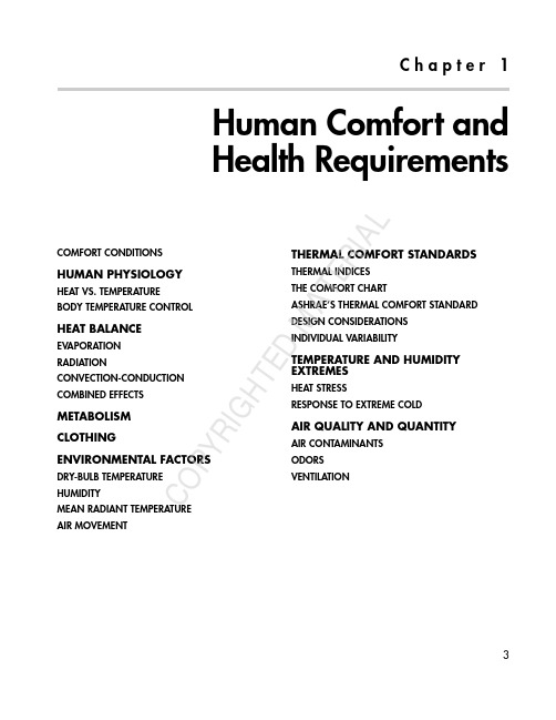
FIGURE 1.1.Physiological reactions to body temperature.surface temperature). The skin also has sensors that signal to the brain the level of heat gain or loss at the skin.It is the hypothalmus that appears to trigger the heat con-trol mechanisms to either increase or decrease heat loss. ThisFIGURE 1.2.Heat balance of the human body interacting with its environment.FIGURE 1.3.Radiant heat transfer with surrounding surfaces.Convection-ConductionAir passing over the skin surface is instrumental not only to the evaporation of moisture,but also to the transference of sensible heat to or from the body. The faster the rate of air the larger the temperature difference between the body and surrounding air,and the larger the body surface the greater the rate of heat transfer.When the air temperature is lower than the skin (and clothing) temperature,the convective heat term in equation becomes increasingly effective at dissipating heat as air tem-perature decreases and air movement increases.The conduction heat loss or gain occurs through contact of the body with physical objects such as the floor and chairs. If two chairs—one with a metal seat and the other with a fabric seat—have been in a 70°F (21°C) room for a period of time,they will both have a temperature of 70 (21°C),but the metal one will feel colder than the one with the woven seat.There are two reasons for this. First,metal is a good con-FIGURE 1.4.Alternative methods of achieving radiant comfort.FIGURE 1.5.Relationship between metabolism,evaporation,radiation,convection,and temperature.FIGURE 1.6.Scale of activity level variations (in met units).FIGURE 1.7.Clothing level (in clo units) necessary for comfort at different operative temperatures. (Reprinted from Standard 55by permission of the American Society of Heating,Refrigerating andAir-Conditioning Engineers,Inc.)Conditions that are thermally acceptable to at least 80 percent of normally clothed occupants are presented in Fig-temperatures can be established almost independently of the variables.There is actually a fairly wide range of tem-that can provide comfort when combined with thecombination of relative humidity,MRT,and air flow.one of these conditions varies,the dry-bulb temper-be adjusted in order to maintain comfort conditions.Temperature drifts or ramps are gradual temperature over time.Drifts refer to passive temperature changes,temperature excursion doesn’t extend far beyond the speci-fied comfort conditions and for very long.Air temperature in an enclosed space generally increases from floor to ceiling. If this variation is sufficiently large, discomfort could result from the temperature being overly warm at the head and/or overly cold at the feet,even though the body as a whole is thermally neutral. Therefore,vent local discomfort,the vertical air temperature differenceFIGURE 1.8.Illustration of a range of clo values.FIGURE 1.9.Sling psychrometer.Answers (English Units)1.MRT =ᎏΣ3T 60θᎏ==62°F(48 ×130) +(67 ×60) +(72 ×170)ᎏᎏᎏᎏ360FIGURE 1.10.Example of MRT calculation.a minimum of 1 hour of exposure,0.6 clo (standard shirt-sleeve indoor office clothing),and a 1-met (seated or seden-tary) activity level. It is secondarily useful at higher temperatures to identify when there is a risk of sedentary heat stress. Although the ET* scale is based on 1-hour expo-data show no significant changes in response with longer exposures unless the limits of heat stress—ET* greater than 90°F (32°C)—are approached. As the ET* lines humidity between about 20 and 55 percent RH has range is only about 25 percent of the total heat loss. As the temperature increases,this percentage grows until the ambi-ent temperature equals skin (and clothes) temperature, which point evaporation accounts for 100 percent of the heat loss.The upper and lower humidity limits on the comfort enve-lope of Figure 1.12 are based on considerations of respira-tory health,mold growth,and other moisture-related phenomena in addition to comfort. Humidification in winterFIGURE 1.11.The ET* scale correlated to physiological reactions,comfort,and health.and air movement necessary for thermal comfort depend upon the occupant’s clothing and activity level. The comfort chart was developed from ASH RAE research, which has usually been limited to lightly clothed occupants (0.5 to 0.6 clo) engaged in sedentary activities. The reason-ing behind this approach is that 90 percent of people’s indoor movement within the occupied zone should not exceed 30 fpm (0.15 m/s). If the temperature is less than the optimum or neutral sensation temperature,slight increases in air velocity or irregularity of air movement can cause uncom-fortable localized drafts. While possibly of little conse-quence in an active factory,this can create significantFIGURE 1.12.The comfort chart.。
- 1、下载文档前请自行甄别文档内容的完整性,平台不提供额外的编辑、内容补充、找答案等附加服务。
- 2、"仅部分预览"的文档,不可在线预览部分如存在完整性等问题,可反馈申请退款(可完整预览的文档不适用该条件!)。
- 3、如文档侵犯您的权益,请联系客服反馈,我们会尽快为您处理(人工客服工作时间:9:00-18:30)。
Chapter 9:
Natural Convection
Yoav Peles
Department of Mechanical, Aerospace and Nuclear Engineering Rensselaer Polytechnic Institute
Copyright ©The McGraw-Hill Companies, Inc. Permission required for reproduction or display.
Objectives
When you finish studying this chapter, you should be able to:•Understand the physical mechanism of natural convection,•Derive the governing equations of natural convection, and obtain the dimensionless Grashof number by nondimensionalizing them,•Evaluate the Nusselt number for natural convection associated with vertical, horizontal, and inclined plates as well as cylinders and
spheres,
•Examine natural convection from finned surfaces, and determine the optimum fin spacing,
•Analyze natural convection inside enclosures such as double-pane windows, and
•Consider combined natural and forced convection, and assess the relative importance of each mode.
Viscous Force Buoyancy Force
g
g
Z
o o m i n dy dt
P
Substituting Eqs. 9–8 and 9–9 into Eq. 9–7 and
conservation of )1
dx dy ⋅⋅
The flow regime in natural convection is Buoyancy force
Viscous force
Empirical
correlations
1010 for Nu
avg
g L c=0.3 m
β ≈1 / T
k = 0.026 W/m-K
0.25
3
0.25
2.714 2.714opt
s L
S L L
S Ra Ra ⎛⎞
==⎜⎟
⎝⎠
(9-32)
WL 量 (T s =constant) :
255
.54)(Ra ; )]
([714
.2]
)
([
714.2s 25
.025
.04
====L
S
S S L
S Ra S
L
S Ra S
S opt s s opt (9-31)
Nu = h S opt / k = 1.307
量= Q = h (2nLH) (T s –T ∞)
(9-34)
(9-33)
n = 數
T ∞
enclosure, the fluid adjacent to the hotter
enclosure
•Gr /Re 2 < 0.1 : natural convection is negligible .•Gr /Re
2 > 10 : forced convection is negligible .•0.1 < Gr /Re 2 <10 : forced and natural convection are
not negligible .
hot isothermal vertical
plate。