Numerical Simulation of Heat Transfer Characteristics of Horizontal Ground Heat Exchanger in Fro
数值传热学 -回复

数值传热学 -回复
数值传热学(Numerical Heat Transfer)是一门研究热传递现象的学科,通过数值模拟和计算方法来分析热传导、对流和辐射等传热过程。
本文将介绍数值传热学的基本原理、方法和应用。
1. 基本原理
数值传热学基于传热学原理和计算数学方法,将传热过程建模为数学方程,并通过数
值方法求解这些方程,从而得到热传递的数值解。
主要的传热模型包括热传导、对流和辐
射传热。
2. 数值方法
数值传热学常用的方法包括有限差分法、有限元法和边界元法等。
有限差分法是最常
用的方法之一,将传热区域离散化为网格,通过差分近似计算网格点上的温度或热流量。
有限元法则是另一种常用的方法,将传热区域划分为元素,通过建立元素之间的关系来计
算温度场或热流场。
边界元法则是将问题转化为边界上的积分方程,通过求解积分方程得
到温度场或热流场。
3. 应用领域
数值传热学在各个领域都有广泛的应用。
在工程领域,数值传热学用于优化热交换器
的设计、预测电子器件温度分布、模拟流体在管道内的传热过程等。
在材料科学领域,数
值传热学用于研究材料的导热性能、相变过程以及焊接和烧结等工艺。
在能源领域,数值
传热学用于分析太阳能热收集器的性能、燃烧过程中的传热机制等。
通过数值传热学的研究,我们可以更加深入地了解热传递过程,并可以通过数值模拟
方法来预测和优化热传递的效果。
数值传热学也为各个领域的工程和科学研究提供了重要
的工具和方法。
通过不断的发展和创新,数值传热学将进一步推动热传递理论和应用的发展。
多层介质传热的计算模拟

摘
*
要
在稳定热源流过多层介质材料的传热过程中,温度会随时间和位置发生变化。本文分析了稳定热源通过
通讯作者。
文章引用: 甄嘉鹏, 郭琦, 周江. 多层介质传热的计算模拟[J]. 应用物理, 2019, 9(1): 7-12. DOI: 10.12677/app.2019.91002
甄嘉鹏 等
多层介质传热的温度分布,运用热传导方程导出了热稳定后的温度分布以及最内层材料温度随时间的变 化关系。本文的方法适用于多种隔热材料的复合问题,可求出多层介质各层温度随时间的变化规律。
Keywords
Multi-Layered Media, Heat Transfer, Thermal Insulation Material
多层介质传热的计算模拟
甄嘉鹏1,郭
1 2
琦2,周
江1*
贵州大学物理学院,贵州 贵阳 贵州大学数学与统计学院,贵州 贵阳
收稿日期:2018年12月21日;录用日期:2019年1月4日;发布日期:2019年1月11日
由傅里叶定律和能量守恒定律得出温度随时间和位置变化的方程[8]:
Open Access
1. 引言
多层材料在传热过程中,不同介质材料会导致不同的温度分布。温度在材料内部随着位置而变化, 材料最内侧的温度会随热传递的时间而变化。 这类问题从 20 世纪 80 年代开始一直被广泛研究。 1981 年, 顾延安研究了保温层外壁面温度,以及它的计算方法,通过理论推导给出了一种计算热损失的方法[1]。 2007 年,白净选用第一类边界条件下的柱坐标形式的导热微分方程对圆筒壁内的温度分布进行计算和分 析,得出结论等温面的热流密度相同[2]。曾剑等考虑了一类热传导方程中间断扩散系数的反问题,证明 了时间相对较小时,极小元的唯一性和稳定性[3] [4] [5] [6]。2018 年,陈大伟利用热传导方程的差分格式 对一维热传导方程的数值解进行计算并绘成图, 从而直观地得到热传导媒介上的温度时空分布[7]。 目前, 对于热传导方程解的研究并以此得到热传导媒介在传热过程中的温度分布的相关研究仍在继续,然而对 于将两者与隔热材料相结合以提高复合材料的隔热性能以及对隔热时间的研究仍然较少。该研究对于复 合材料隔热性能的提高和隔热材料的选择具备参考价值,在实际生活中的应用也较为广泛,可应用于高 温作业服、消防隔热墙等诸多领域,因此具有一定的研究价值。 本文通过实验所得实验数据,利用数学物理方程建立稳定状态下的温度分布模型,包括复合介质各 分界面的温度变化和多层材料内侧温度随时间的变化。将该热传导模型和实验曲线进行对比,验证模型 的正确性。
Mathematical Modeling of Heat Transfer
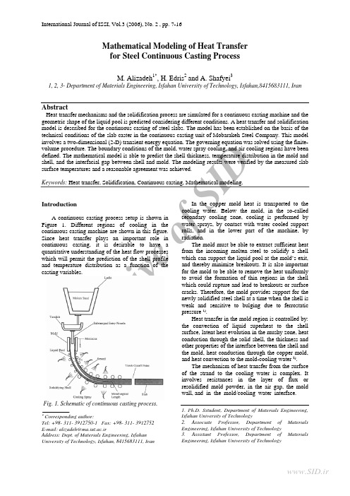
A rc hi v eo fSI DMathematical Modeling of Heat Transfer for Steel Continuous Casting ProcessM. Alizadeh 1*, H. Edris 2 and A. Shafyei 31, 2, 3- Department of Materials Engineering, Isfahan University of Technology, Isfahan,8415683111, IranAbstractHeat transfer mechanisms and the solidification process are simulated for a continuous casting machine and the geometric shape of the liquid pool is predicted considering different conditions. A heat transfer and solidification model is described for the continuous casting of steel slabs. The model has been established on the basis of the technical conditions of the slab caster in the continuous casting unit of Mobarakeh Steel Company. This model involves a two-dimensional (2-D) transient energy equation. The governing equation was solved using the finite-volume procedure. The boundary conditions of the mold, water spray cooling, and air cooling regions have been defined. The mathematical model is able to predict the shell thickness, temperature distribution in the mold and shell, and the interfacial gap between shell and mold. The modeling results were verified by the measured slab surface temperatures and a reasonable agreement was achieved.Keywords: Heat transfer, Solidification, Continuous casting, Mathematical modeling.IntroductionA continuous casting process setup is shown inFigure 1. Different regions of cooling in the continuous casting machine are shown in this figure.Since heat transfer plays an important role incontinuous casting, it is desirable to have aquantitative understanding of the heat flow processeswhich will permit the prediction of the shell profileand temperature distribution as a function of thecasting variables.Fig. 1. Schematic of continuous casting process.∗Corresponding author:Tel: +98- 311- 3912750-1 Fax: +98- 311- 3912752 E-mail: alizadeh@ma.iut.ac.irAddress: Dept. of Materials Engineering, Isfahan University of Technology, Isfahan, 8415683111, IranIn the copper mold heat is transported to the cooling water. Below the mold, in the so-called secondary cooling zone, cooling is performed by water sprays, by contact with water cooled supportrolls, and in the lower part of the machine, by radiation. The mold must be able to extract sufficient heat from the incoming molten steel to solidify a shell which can support the liquid pool at the mold’s exit, and thereby minimize breakouts. It is also important for the mold to be able to remove the heat uniformly to avoid the formation of thin regions in the shell which could rupture and lead to breakouts or surface cracks. Therefore, the mold provides support for the newly solidified steel shell at a time when the shell is weak and sensitive to bulging due to ferrostatic pressure 1).Heat transfer in the mold region is controlled by: the convection of liquid superheat to the shell surface, latent heat evolution in the mushy zone, heat conduction through the solid shell, the thickness and other properties of the interface between the shell and the mold, heat conduction through the copper mold, and heat convection to the mold-cooling water 2).The mechanism of heat transfer from the surface of the strand to the cooling water is complex. It involves resistances in the layer of flux or resolidified mold powder, in the air gap, the mold wall, and in the mold/cooling water interface.1. Ph.D. Sstudent, Department of Materials Engineering, Isfahan University of Technology2. Associate Professor, Department of Materials Engineering, Isfahan University of Technology3. Assistant Professor, Department of Materials Engineering, Isfahan University of TechnologyA rc hi v eo fSI DInternational Journal of ISSI, Vol.3 (2006), No. 2Table 1: Comparison of thermal conductivities of materials present in the continuous casting mold [3].MaterialsTemperature(o C) Thermal conductivity(W m -1 K -1)Steel St 37 1200 29 Copper 30-130 385 Casting flux 1000-1300 0.5 to 1.2 Water 25 0.62Radiation conductivity of gas gap 1000 0.043Fig. 2. Different regions and simulation domain in continuous casting process.The thermal conductivities of different layers are compared in Table 1. As shown in this table, the air gap has the largest resistance to heat flow, while the other parts have a comparatively small resistance. Therefore, the pattern of heat removal in the mold is dependent largely upon the dynamics of gap formation. The air gap or contact resistances can be generated by the shrinkage of the steel shell away from the mold walls, especially after the flux is completely solid and unable to flow into the gaps. More researches were performed to show that the air gap was usually created in the lowest one-third of the mold length 3).In the upper part of the secondary cooling zone, the strand is usually sprayed by water emerging from nozzles arranged in the spaces between the rolls. The rate at which heat is extracted from the strand surface by water sprays has been measured by many researchers. These researchers have shown that under normal continuous casting conditions, in which shell surface temperatures range between 700 and 1200 o C, surface temperature has a little effect on the heat transfer coefficient. All studies agree that, in the stated temperature range, the spray water flux has the most effect on the heat transfer coefficient. Moreover, the temperature of sprayed water does not have a large influence on the heat transfer coefficient 4).In the lower part of the secondary cooling zone, heat transfer is preferred mainly by radiation and by roll contact. Therefore, it should be considered that the oxide scales generated on the surface of the strand could cause a thermal resistance in this zone 5).In this study, the mathematical model has been established on the basis of the technical conditions of the slab caster in the continuous casting unit of Mobarakeh Steel Company. In this model, steel heat capacity and steel thermal conductivity were considered as functions of steel temperature and chemical composition. Considering these functions, the governing equation is a non-linear equation. In this study the equation is solved in non-linear state. This model is also capable of predicting the temperature distribution, including the solidus and liquidus isotherm which defines the solid shell and mushy zone, respectively, as a function of section size, pouring temperature, steel composition, casting speed, mold length and spray conditions.Mathematical modelingFigure 2 shows the different regions of the continuous casting machine and the model considered for physical simulation of the caster. A typical method of modeling the strand thermal condition is shown in this figure. The mathematical model is applied to slices of strand that start at the meniscus and travel through the machine at the casting speed. New slices are generated periodically. A sufficient number of slices exist in each cooling zone to give an accurate representation of the thermal condition in each zone. In this model, only a quarter of the strand is considered due to the symmetry of the heat flow conditions (Figure 3).A rc hi v eo fSI DInternational Journal of ISSI, Vol.3 (2006), No. 2Fig. 3. A symmetric quarter of strand width section with physical coordinate.AssumptionsThe following assumptions are made to simplify the mathematical model 6):-Conduction can take place only in the transverse directions.-Forced convective heat flow in the liquid pool is considered by defining an effective liquid thermal conductivity as:l eff K K ⋅=7(1) -The density of steel is constant, but specific heatcapacity and heat conductivity of steel are functions of temperature and chemical composition and therefore not constant.Model formulationThe energy conservation equation can be written as 7):(2)()()()()⎟⎠⎞⎜⎝⎛∂∂∂∂+⎟⎟⎠⎞⎜⎜⎝⎛∂∂∂∂+⎟⎠⎞⎜⎝⎛∂∂∂∂=∂∂+∂∂+∂∂+∂∂z T k z y T k y x T k x wH vH y uH x H t effeffeffρρρρ To simplify the equation, a transformation as wt z −=ζ is used. Therefore this is: (3)()ls ls s sH H H t y x H H q tHy H y x H x tH +==+∂∂−⎟⎟⎠⎞⎜⎜⎝⎛∂∂∂∂+⎟⎠⎞⎜⎝⎛∂∂∂∂=∂∂;,,,;0ζρααIn order to solve the governing equation, it is necessary to transform the physical domain into a computational domain. In general, this sort of transformation is used, and leads to a uniformly spaced grid in the computational domain but the points in physical domain may be unequally spaced. The original partial differential equation is transformed from physical coordinates (x, y ) to computational coordinates (ξ,η) by applying the chain rule of partial derivatives.;JS H H J H t x y s y x s s +⎟⎟⎠⎞⎜⎜⎝⎛∂∂∂∂+⎟⎟⎠⎞⎜⎜⎝⎛∂∂∂∂=⎟⎠⎞⎜⎝⎛∂∂ξηηαηηξξαξ (4);tH S l ∂∂−= y x J ηξ= In the above equations "S " is a term for heat source due to the metal phase transformation (liquid to solid). In order to establish the region of phase change, the latent heat contribution is specified as a function of temperature i.e. 8):f l l L f H ⋅=(5) Where L f is the latent heat of the phase changeand the liquid fraction (f l ) is computed by:⎪⎪⎭⎪⎪⎬⎫⎪⎪⎩⎪⎪⎨⎧≤≥≥−−≥=.......01sol sol liq sol liq sol liq l T T when T T T when T T T T T T when f (6)A typical 2D cartesian control volume is shownin Figure 4. This C.V contains a central node (P) with four neighborhood points (E, W, N, and S). The integral form of equation (4) is obtained on the control volume by the finite volume method 9,10): a P H sP = a E H sE + a W H sW + a N H sN + a S H sS + b (7) a P = a W + a E + a S + a N + a P oa E =ey x e ⎟⎟⎠⎞⎜⎜⎝⎛ΔΔηξξηα a W =wyx w ⎟⎟⎠⎞⎜⎜⎝⎛ΔΔηξξηα a N =nx y n ⎟⎟⎠⎞⎜⎜⎝⎛ΔΔξηηξα a S =sx ys ⎟⎟⎠⎞⎜⎜⎝⎛ΔΔξηηξαa P o =PJ t ⋅ΔΔ⋅Δηξ b = a P o (H sP o + H lP o - H lP ) + o Pq J ρηξΔ⋅Δ (8)Fig. 4. A typical control volume and the notation used for a Cartesian 2D grid [9].To approximate the variable values on the surface of the control volume, the Quadratic Upwind Interpolation (QUICK) algorithm is used 9). In the QUICK scheme, the variable profile between two points approximated by a parabola instead of aArc hi v eo fSI DInternational Journal of ISSI, Vol.3 (2006), No. 2straight line (Figure 5), on a uniform Cartesian grid leads to 9):W E P e φφφφ818386−+= (9)Fig. 5. Approximation of gradients at cell faces [9].Boundary conditionsTo solve the above equation, the boundary conditions are needed for different regions include the mold, water spray cooling, and air cooling. Figure 6 shows some machine cooling layouts while the technical information belonging to each zone is shown in Table 2. A general form of the boundary condition can be expressed through an equation (10), in which the heat transfer coefficient, h , is estimated for different cooling zones.()water b b T T h n T k −=∂∂−| (10)To determine the temperature of the boundaries, the discretion of the bnT |∂∂ on boundary points isrequired. According to the QUICK scheme b nT |∂∂could be calculated by the following correlation [10]: nT T T nT W P b bΔ+−=∂∂398(11)Therefore, as seen in equation (10), finding the heat transfer coefficient for different regions such as: mold, water spray, and air cooling is necessary.Fig. 6. Secondary cooling of the slab caster.In the mold, several thermal resistance layers exist between the steel shell surface and the recirculation water. All the thermal resistances in the mold are shown in Figure 7. The effective thermal resistance of the water channel is estimated from the water channel heat transfer coefficient, thermal conductivity and the thickness of scale deposits on the surface of the cooling-water channel 11):⎟⎟⎠⎞⎜⎜⎝⎛+=w scale scale water h k d r 1 (12)Fig. 7. Thermal resistances existing between the shell surface and water channel in the mold.Table 2. Secondary cooling zones variables.No. Zone Length zone(m)SegmentNumber of spray nozzles Water flow rate(m 3/sec)Number rollin zoneRoll radius (m)1 0.439 - -2 0.220 - -3 0.303 - 30 0.003975 - -4 0.925 0 38 0.004967 5 0.140 5 1.470 0 38 0.0048426 0.200 6 1.475 1 10 0.004858 5 0.2507 1.725 2 10 0.003975 5 0.3008 1.725 3 10 0.003733 5 0.3009 3.950 4,5 20 0.005667 10 0.350 10 5.200 Roll 37-47 22 0.006483 11 0.380,0.440 11 9.400 Roll 48-63 - Air cooling 16 0.440A rc hi v eo fSI DInternational Journal of ISSI, Vol.3 (2006), No. 2 The heat transfer coefficient between the water and the side walls of the water channel (h w ) is calculated assuming a turbulent flow through an equivalent-diameter pipe (D ) using the empirical correlation of Sleicher and Reusse 11):()21Pr Re 015.05c c water w Dkh += (13)()Pr 6.0215.0333.0;Pr 424.088.0−+=+−=e c cOther thermal resistances shown in Fig 7 can be calculated by the following correlations [11]:;;slag slag slag moldmold mold k d r k dr == ;air air air k d r = (14)Which d slag can be found from the powder consumption per mass of product (M slag (kg/ton)): ()N W N W M d slagsteel slag slag +×××=2ρρ (15) Also, d air includes a gap due to shrinkage of the steel shell, which can be calculated by the thermal linear expansion relation of steel using following correlation for each control volume: T l l Δ⋅⋅=Δλ (16) Where, λ is linear thermal expansion coefficient of steel and l is length of each control volume. Moreover, the heat transfer coefficient due to radiation is calculated by: ()()212221T T T T h rad ++=εσ (17) Heat transfer mechanisms in the spray cooling zones below the mold are defined in Figure 8. The heat extraction due to the water sprays is a function of the water flux. The relationship between the rate of heat extraction by the water sprays and the spray variables has been established in a number ofexperimental studies. One of the most widely usedrelations has been presented by Nozaki's 12): ();0075.013925.055.0water water spray T Q h ×−××= (18)Fig. 8. Heat transfer mechanisms in the secondarycooling zones [12].Due to the high temperature of the strand surfaceand the exposure of water to the surface, an oxidescale is produced on the surface of the strand. Despite the low thickness, the scale can have animportant role in the heat transfer control. Therefore,the effective heat transfer coefficient should be considered as 12):sprayscsceff h k h 11+=δ (19)It has already been mentioned that the cooling ofthe strand in the lower part of the secondary cooling zone is mainly done by radiation 12). Therefore, the equation for the heat transfer coefficient is given as follows:()().2.2am s am s rad T T T T h ++=εσ (20) Besides the radiation, heat transfer is alsoachieved by natural convections, but this part is rather small and can be neglected in comparison to radiation cooling.The symmetrical boundary condition has been considered for midplanes as follows:0.,00.,0=∂∂−==∂∂−=yTk y xTk x (21)Computation and verificationThe algebraic equation of the boundary conditions has been solved with a Tridiagonal Matrix Algorithm (TDMA) solver 13). As seen in equations(7) and (8), to solve the algebraic equation, it is necessary to know the latent enthalpy in a new time step (H l ). To update the amount of the latent enthalpy an iterative solution is used for each time step:11++−+=k sP k sP k lP k lP H H H H (22)As seen in the above equation, by using the sensitive enthalpy that has been obtained by solving the energy equation (H sP k+1), latent enthalpy could be updated in the k+1th inner iteration in each time stepto achieve a certain convergence. The calculation mentioned has been programmed in the FORTRAN language. The mathematic simulation starts by setting the initial steel temperature at the pouring temperature. Input parameters, in Table 3, in the standard cases are verified by the measured temperatures on the shell surface of the strand.Equilibrium lever-rule calculations are performed on a Fe-C phase diagram in order to calculate steel phase fractions. By this means, phase field lines are specified as simple linear functions of carbon equivalent content. The carbon of the steel is applied as the carbon equivalent content that is calculated by the following correlation 14): wt%CE=wt%C+0.04(wt%Mn)-0.14(wt%Si)-0.04(wt%Cr)-0.1(wt%Mo)-0.24(wt%Ti)+0.1(wt%Cu) For a 0.16%C, 1.3%Mn, 0.5%Si, 0.05%Cr, 0.03%Mo and 0.01%Ti plain carbon steel, the carbon equivalent percentage calculated as 0.135 and also the equilibrium phase diagram model calculates T liq.=1528 o C, T sol = 1494 o C. The solid fraction-A rc hi v eo fSI DInternational Journal of ISSI, Vol.3 (2006), No. 2temperature curve in the mushy zone obtained from the model is shown in Figure 9. As seen in this figure the relation between temperature and solid fraction of steel in the mushy zone is non-linear.Solidified shell thickness is one of the most important calculated parameters in the model, and the influence of the grid spacing on this parameter should be considered. The influence of the gridspacing on the solidified shell thickness, in exit point of the mold, is shown in Table 4. The thickness amounts in width and narrow sides are presented in this table. It is clear from Table 4 that when grid spacing is reduced, solidified thicknesses are changed and they are stable in a narrow limit with reduction of grid spacing lower than a certain limit. It can be concluded that the solidified shell thickness is independent of the mesh size with the reduction of grid spacing lower than a certain limit.The mold zone is a complex and important area in continuous casting machine. The solid shell growth in this zone is complicated and the results of this study are compared to those of some other researchers. The comparison between the results of the model in this study and experimentalmeasurement by some other researchers is shown in Figure 10. The figure shows the variation of growth of the solid shell thickness on the ingot for low carbon steel (0.06% C). It is clear that the results from numerical solution in this study have a very good compatibility with those of three 3-D model of Thomas and experimental measurement of Alberny and co-worker.Table 3. Input data for standard conditions.Carbon equivalent content, CE pct 0.132 pctSteel density, ρ7500 kg/m 3 Steel emissivity, ε0.8 Mold copper plates thickness 0.043×0.030 m ×m Total mold length 0.704 m Mold copper plates width 2.220×0.215 m ×m Scale thickness on the surface of mold cold face 0.00001 m Mold conductivity, k mold 315 W/mK Mold powder conductivity, k slag 1.27 W/mK Air conductivity, k air 0.083 W/mKMold powder density, ρslag0.650 kg/m 3 Mold powder consumption rate, M slag 0.8 kg/ton steel Casting speed, V c 0.0167 m/secPour temperature, T in 1546 oCLiquidus temperature, T liq. 1528.6 oCSolidus temperature, T sol. 1494 oC Working mold length 0.659 m Slab geometry, W ×N 1.250×0.203 m ×m Scale conductivity on the surface of slab, k sc 0.5 W/mK Scale conductivity on the surface of mold, k scale 1.0 W/mK Water channel geometry, large & small plates 25×5×29 & 22×5×26mm 3 Average cooling water temperature in the mold 28 oC Water flow rate entering the mold small plate, 0.0061 m 3/sec Water flow rate entering the mold large plate, 0.0553 m 3/sec Latent heat of the steel phase change, L f 272140 J/kgWater conductivity , k water0.615 W/mKSteel specific heat capacity [11], C p ()()()()⎪⎪⎪⎪⎪⎪⎭⎪⎪⎪⎪⎪⎪⎬⎫⎪⎪⎪⎪⎪⎪⎩⎪⎪⎪⎪⎪⎪⎨⎧≥=≤=≤+=≤=−==+=+=liqp liq sol p sol op p o p p op o p T T C T T T C T T C T C T C T C T C T C T C T C T C T C 7877721100*334.02681100850648850750*766.338497507001431700500*836.0268500*376.0456p p p p p p p p p p J/kgK Steel conductivity, k steelf l *k liq +(1-f l )*k sol W/mK Solid steel conductivity, k sol 33.0 W/mK Effective molten steel conductivity, k liq 7*43.0 W/mKScale thickness on the surface of slab , δsc0.001 mA rc hi v eo fSI DInternational Journal of ISSI, Vol.3 (2006), No. 2Table 4. Effect of mesh size on the shell thickness at mold exit.Grid system #nx ×n y Shell thickness at middle of wide face (m)Shell thickness at middle of narrow face (m)25×10 0.0145 0.0111 25×15 0.0135 0.0110 50×15 0.0136 0.0118 50×20 0.0133 0.0119 100×200.0136 0.0117 100×300.0131 0.0117Fig. 9. Phase fraction variation with temperature in mushy zone.Fig. 10. Comparison between model results and other references.Results and discussionThe calculated surface temperatures of a slab, for the Table 3 conditions as a function of the distance below the meniscus, are presented in Figure 11. This figure shows the calculated surface temperatures at the centers of the wide and narrow faces and at the corners of the slab caster. The central areas of the wide faces are cooled one-dimensionally, whereas the slab corners are subject to 2-D cooling. The slab corners can therefore become significantly colder than other parts of the inner wide face. At the beginning of straightening, the slab corner temperature is 230 o C less than the temperature at the center of the wide face. Control of corner cooling is critical for much of continuously cast products. The slab corners tend to have meniscus marks, which act as stress risers. A combination of temperature, stress risers and a low ductility region in the 700-900 o C temperature range during the straightening process often leads to cracks in the corners. One way to increase the corner temperature is to widen the strip of unsprayed strand at the corner. However, as the non-sprayed strip is widened, a hot spot will develop between the colder corner and the sprayed area. Thus, the design must be in a way to ensure that it does not cause other quality problems. Also, as seen in Figure 11, the intensity of heat transfer of mist spray cooling is less than cooling in the lower part of the mold for all of the curves, because of this, the model predicts a 200 o C reheating of the slab surfaceon leaving the mold. A similar situation also exists in water spray cooling and air cooling regions on the surface of the wide face slab.Fig. 11. Predicted surface temperature of strand. Figure 12 shows the solidified shell thickness profiles of both the narrow and wide faces of the slab. This figure shows a sudden change of slope at the beginning of the solidified shell growth curve. It is indicated that the rate of solidified shell growth is clearly high in the mold region. Figure 13 shows a set of data of the local heat flux density along the length of the mold [15]. There is a maximum of heat flux density somewhat below the meniscus. Downward, the heat flux density usually decreases. If the air gapA rc hi v eIDInternational Journal of ISSI, Vol.3 (2006), No. 2between the mold and strand approximately has uniform thickness, or it increases uniformly in the downward direction, the heat flux density along the length of the mold continuously decreases.Fig. 12. Predicted solidified shell thickness.Fig. 13. Heat flux density distribution along the length of the mold.Fig. 14. Effect of casting speed on the pool depth.The casting speed is the most effective parameter in changing the position of the solidified shell thickness profiles. The relation of the "metallurgical length" (maximum length of the liquid pool) with the casting speed is shown in Figure 14. Increase in casting speed decreases the holding time of the slab in the secondary cooling zones and increases the length of the liquid core. Therefore, casting speed is the most important factor in controlling mold heat extraction. The solidified shell thickness as a function of the casting speed of bothwide face and narrow face of the strand are shown in Figure 15. Since, a lower casting speed provides more time for the heat to be extracted from the shell, the shell thickness increases. Moreover, the shell thickness in the initial solidification stage decreases at the high casting speed, as shown in Figure 15, which often easily causes the breakout of strand. Therefore, to prevent this unfavorable defect, the casting speed is limited. It should be mentioned that steel composition and slab width in comparison to casting speed has no significant effect on the shell thickness. As seen in this figure, solidified shell thickness for wide face is higher than it is for narrow face. This is because of the different air gap sizes between mold powder and mold wall in both wide and narrow faces. The air gap size along the length of the mold is predicted by the model for both faces in Figure 16. As seen in this figure, total shrinkage value in narrow face is more than wide face as expected because width size of slab is much larger than thickness size in cross section of strand. Furthermore, this phenomenon could change Fig. 15. Effect of casting speed on shell thickness.Fig. 16. air gap size along the mold.Heat transfer in the mold is governed by these three resistances: the casting-mold interface, the mold wall, and the mold-cooling water interface. Although, thermal resistance due to the air gapA rc hi v e o fSI DInternational Journal of ISSI, Vol.3 (2006), No. 2 should also be considered while the amount of air gap thermal resistance is usually quite large compared to the other resistances especially for the lower portion of the mold. Temperatures of three points: slag layer/mold wall interface (T 1), mold wall (T 2), and water channel wall (T 3) as shown in Figure 7 are predicted by the model. Since, the heat flux for steady state conditions will be constant and independent of distance: (23)mold rad airradair slag s rad airrad air slags slags total water s r rr r r r T T rr r r r T T r T T r T T q +⎟⎟⎠⎞⎜⎜⎝⎛+⋅+−=⎟⎟⎠⎞⎜⎜⎝⎛+⋅+−=−=−=′321The above relation represents three equations for the three unknowns, T 1, T 2, and T 3. The results of the model predictions are shown in Figure 17(a) and Figure 17(b). As seen in these figures, the existence of the air gap between the shell surface and mold wall causes the T 1 to increase both in wide and narrow faces of strand. Since the air gap thickness in the narrow face is larger than the wide face, T 1 in the narrow face is much higher than in the wide face. Therefore, the pattern of heat removal in the mold is dependent largely upon the dynamics of gap formation. It causes temperature difference to exist in solidified shell and has a strong influence on transverse cracks generation in the mold region.Fig. 17. Predicted temperatures for T 1, T 2 and T 3 points in Fig 7 -(a) wide face and (b) narrow face (T 1=slag layer/mold wall interface temperature, T 2=mold wall temperature, and T 3=water channel wall temperature).The effect of the amount of superheat temperature of the molten steel, entering the mold, on the solidified shell thickness is shown in Figure 18. At first, with increasing the superheat temperature, the superheat flux will increase and therefore, the solidification rate decreases. This, in turn, reduces the thickness of the steel shell. On the other hand, by increasing the superheat temperature, the driving force for the heat transfer will increase. Therefore, as seen in Figure 18, the influence of the superheat temperature is insignificant to shell growth, especially in the wide face of the strand. Low superheat, near liquidus temperature, is beneficial to continuous casting. Internal quality is improved as the equated zone is made significantly larger. Therefore, a more desirable structure with greater resistance to halfway cracks is produced. Centerline segregation and porosity are also reduced or eliminated.Fig. 18. Effect of steel superheat temperature on the shell thickness at mold exit.Conclusions1- A finite volume heat transfer and solidification model has been formulated to predict the temperature field and liquid pool position in the continuous casting process under different conditions. This has been verified with the temperature measurement of slab surface.2- Casting speed is the most effective parameter on mold heat removal. Therefore, it is the most important factor in controlling solidified shell thickness and slab temperature.3- Since, the air gap size in narrow face of mold is higher than the wide face, the breakout of strand often occurs in the narrow face.4- Air gap existing in the casting-mold interface causes a large thermal resistance for heat transfer from the solidified shell to the mold. Therefore, it has a strong influence on product quality and casting problems, especially for the narrow face of strand. 5- High superheat temperature may cause breakouts at the mold exit, especially for the narrow face, so it should be exactly kept at a low level.。
多孔纤维织物热湿传递数值模拟的研究进展

多孔纤维织物热湿传递数值模拟的研究进展王红梅;郑振荣;张楠楠;张玉双;赵晓明【摘要】Research of numerical simulation of heat and moisture transfer can provide theoretical foundation for the preparation and heat⁃moisture properties evaluation of porous textiles. Based on the heat and moisture transfer mechanism, new progress of the heat and moisture transfer through fabrics was summarized in terms of heat and moisture transfer models, numerical simulation methods and test methods of fabricheat⁃moisture transport properties, and the problems existing in the numerical simulation of heat and moisture transfer in fabric were analyzed. Taking into consideration interweave structure characteristics of fabric and the physical properties of the yarn was proposed when coupled heat and moisture transfer model established in three⁃dimensionl. In addition, the change of material physical properties depending on practical application conditions was considered in the process of numerical analysis, heat and moisture transfer numerical model of fabric need further optimize and the improvement of the accuracy.%热湿传递数值模拟的研究可为多孔纤维织物的制备和热湿性能评估提供理论基础。
PO6016《湍流两相流动的模化与数值仿真》 课程教学大纲

2、掌握两相流的相似理论及模化方法,具备对两相流工程实际问题进行模 化设计与相似分析的能力。(A5.1、A5.4、B2、B4.1、B4.2)
的应用”和“基于数值仿真的热力新产品开发”,并开展课程陈述与讨论。通过面 向解决实际工程问题的课程实践,能够开拓学生的思路,教会他们运用理论知识 和科学的研究方法解决实际的科学技术问题,进行严格的科研训练和具备良好的 科研素质。
专题讲座 本课程将设置三次专业讲座,并通过工程案例分析具体讲解湍流两相流动的 模化方法和数值仿真技术,包括两相流模化方法、两相流数值仿真技术及其在工 程设计与产品开发中的应用。 四、考核与评估 课程得分比例如下:
1
课堂出席
10%
2
个人作业
15%
3 大作业(专题研究)
60%
4
课程陈述与讨论
15%
课堂出席 学生课堂出席成绩根据学生在课堂上的表现确定,包括出席、讨论、课堂练 习和表现等。评价课堂出席情况的标准包括参加者是否很好地倾听课程、能否积 极地参与课堂讨论、参加者的表达是否简洁和明确、能否有见地的分析案例和提 供清楚的论证。 个人作业 本课程在重点章节布置 4-6 次课后作业,主要是巩固已学基本概念和基本理 论,并运用基本知识解决关键问题,也推荐学生阅读经典的科技文献和综述。根 据作业完成情况和正确性评定成绩。 大作业(专题研究报告) 大作业(专题研究报告)是针对能源动力两相流工程实际问题开展专题研究,
出版商:
科学出版社
出版年:
1994
参考书目: Clement Kleinstreuer. Two-Phase Flow: Theory and Application, Taylor & Francis Group, New York, London, 2003 ISBN: 1-59169-000-5
超临界压力CO_2在垂直管内对流换热数值模拟
第43卷第3期原子能科学技术Vol.43,No.3 2009年3月Atomic Energy Science and TechnologyMar.2009超临界压力CO 2在垂直管内对流换热数值模拟李志辉,姜培学(清华大学热能工程系热科学与动力工程教育部重点实验室,北京 100084)摘要:对于超临界压力CO 2在垂直圆管(d in =2mm )内高进口雷诺数(Re =9000)条件下向上流动时的对流换热进行了数值模拟。
通过与实验数据进行对比来验证湍流模型的可靠性,并研究变物性和浮升力对壁面温度和湍动能的影响。
结果表明:在热流密度较高的情况下,向上流动时出现了局部换热恶化和换热强化现象,这主要归因于浮升力对湍动能分布的影响;采用LB 湍流模型能较好地模拟这种换热现象;在热流密度较低的情况下,未出现上述换热现象。
关键词:超临界压力;浮升力;换热恶化;数值模拟中图分类号:T K124 文献标志码:A 文章编号:100026931(2009)0320247205Numerical Simulation of Convection H eat T ransfer for CO 2at Supercritical Pressure in V ertical Circular TubeL I Zhi 2hui ,J IAN G Pei 2xue(Key L aboratory f or T hermal S cience and Pow er Engineering of M inist ry of Education ,De partment of T hermal Engineering ,Tsinghua Universit y ,B ei j ing 100084,China )Abstract : Convection heat t ransfer of CO 2at supercritical p ressure in a vertical circular t ube (d in =2mm )at high inlet Re (about 9000)was investigated numerically to analyze t he effect s of t he variatio n of t he p hysical p roperties and buoyancy on t he wall tempera 2t ure and t he t urbulent energy.The result s show t hat in t he case of high heat fluxes t he local heat t ransfer deterioration and enhancement during t he upward flow due to t he st rong influence of buoyancy result in change of t he t urbulent energy dist ribution.Simulations using t he LB t urbulence model correspo nd well wit h t he experimental data in upward flow.In t he case of low heat fluxes t he p henomenon of heat transfer deterioratio n or enhancement was not observed.K ey w ords :supercritical pressure ;buoyancy ;deterioration ;numerical simulation收稿日期:2007212201;修回日期:2008203220基金项目:教育部科学技术重大项目资助(306001);国家“863”计划资助项目(2006AA05Z416)作者简介:李志辉(1976—),男,山西晋城人,博士研究生,动力工程及工程热物理专业 从20世纪五、六十年代开始,国内外学者对超临界流体在管道中的对流换热已进行了大量的实验和理论研究[124]。
Mathematical Model for Fluid Flow and Heat Transfer in the Cooling Shaft of

Cpf Cp~ dp dh F ks K g h~f m n nx ny p qw q~ r r R0 RI S t t, ty Tf T~ uf Us ut vf vs v~ V Vf
general transport equation fluid specific heat, (J/(kg K)) solid specific heat, (J/(kg K)) particle diameter, (m) hydraulic diameter of the passage of gas flow, (m) inertial coefficient, dimensionless the coefficient of solid flow potential permeability, (mz) gravitational acceleration, -9.81, (m2/s) fluid-solid heat transfer coefficient, (W/(m 2 K)) mass flux through a control volume face unit outward normal vector the x -direction component of n the y -direction component of n fluid pressure, (Pa) heat flux at the wall, (W/m 2) source term the position vector radial coordinate, (m) the diameter of prechamber, (m) the diameter of the cooling chamber, (m) the surface area of cell face, (m2) unit vector tangential to the boundary. the x -direction component of t the y -direction component of t fluid temperature, (K) solid temperature, (K) Darcy velocity in x direction, (m/s) the coke descending velocity in x direction, (m/s) velocity vector component in t -direction Darcy velocity in r direction, (m/s) the coke descending velocity in r direction, (m/s) velocity vector component in n -direction, (m/s) velocity vector, (m/s) gas velocity vector, (m/s)
cfx计算共轭传热
cfx计算共轭传热英文回答:Conjugate heat transfer refers to the simultaneous transfer of heat between a solid body and a fluid medium. This phenomenon is commonly encountered in various engineering applications, such as cooling systems, heat exchangers, and combustion chambers. The understanding and analysis of conjugate heat transfer are crucial for designing efficient and reliable thermal systems.One approach to calculate conjugate heat transfer is by using the computational fluid dynamics (CFD) method. CFD is a numerical technique that solves the governing equations of fluid flow and heat transfer. In the case of conjugate heat transfer, the equations for fluid flow and heat transfer in the fluid domain and solid domain are coupled together.To perform a CFD simulation of conjugate heat transfer,the first step is to discretize the fluid and solid domains into smaller control volumes or finite elements. The governing equations, such as the Navier-Stokes equationsfor fluid flow and the heat conduction equation for solid, are then numerically solved within each control volume or finite element. The boundary conditions, such as the fluid velocity and temperature at the inlet and outlet, as wellas the solid surface temperature, need to be specified.The solution procedure involves iterating between the fluid and solid domains until convergence is achieved. In each iteration, the fluid properties, such as the density and viscosity, are updated based on the fluid temperature obtained from the previous iteration. The heat transfer between the fluid and solid is accounted for by considering the convective heat transfer coefficient and thetemperature difference between the fluid and solid surfaces.Conjugate heat transfer simulations can providevaluable insights into the heat transfer characteristicsand temperature distribution within a system. For example,in the design of a heat exchanger, the simulation resultscan help optimize the geometry and determine the required fluid flow rate to achieve the desired heat transfer rate. In a combustion chamber, the simulation can predict the temperature distribution on the solid walls and ensure that the materials can withstand the high temperatures.In addition to CFD, another approach to calculate conjugate heat transfer is through the use of analytical methods. Analytical solutions can be derived for simplified geometries and boundary conditions, allowing for a more straightforward and efficient calculation of heat transfer. However, analytical solutions are often limited toidealized scenarios and may not capture the complex flow and temperature patterns seen in real-world applications.In conclusion, conjugate heat transfer is a critical phenomenon in various engineering applications. The calculation of conjugate heat transfer can be performed using computational fluid dynamics or analytical methods. Both approaches have their advantages and limitations, and the choice of method depends on the specific problem and available resources.中文回答:共轭传热是指固体体和流体介质之间同时进行的热量传递。
数值传热学

数值传热学数值传热学(numerical heat transfer)数值传热学,又称计算传热学,是指对描写流动与传热问题的控制方程采用数值方法,通过计算机求解的一门传热学与数值方法相结合的交叉学科。
数值传热学的基本思想是把原来在空间与时间坐标中连续的物理量的场(如速度场,温度场,浓度场等),用一系列有限个离散点上的值的集合来代替,通过一定的原则建立起这些离散点变量值之间关系的代数方程(称为离散方程)。
求解所建立起来的代数方程已获得求解变量的近似值。
数值传热学(numerical heat transfer)数值传热学,又称计算传热学,是指对描写流动与传热问题的控制方程采用数值方法,通过计算机求解的一门传热学与数值方法相结合的交叉学科。
数值传热学的基本思想是把原来在空间与时间坐标中连续的物理量的场(如速度场,温度场,浓度场等),用一系列有限个离散点上的值的集合来代替,通过一定的原则建立起这些离散点变量值之间关系的代数方程(称为离散方程)。
求解所建立起来的代数方程已获得求解变量的近似值。
数值传热学常用的数值方法1.有限差分法历史上最早采用的数值方法,对简单几何形状中的流动与换热问题最容易实施的数值方法。
其基本点是:将求解区域中用于坐标轴平行的一系列网格的交点所组成的点的集合来代替,在每个节点上,将控制方程中每一个导数用相应的差分表达式来代替,从而在每个节点上,形成一个代数方程,每个方程中包括了本节点及其附近一些节点上的未知值,求解这些代数方程就获得了所需的数值解。
2.有限容积法将所计算的区域划分成一系列控制容积划分为一系列控制容积,每个控制容积都有一个节点做代表。
通过将守恒型的控制方程对控制容积坐积分导出离散方程。
在导出过程中,需要对界面上的被求函数本身及其一阶导数的构成做出假定,是目前流动与换热问题的数值计算中应用最广的一种方法。
3.有限元法把计算区域划分为一系列原题(在二维情况下,元体多为三角形或四边形),由每个元体上去数个点作为节点,然后通过对控制方程做积分来获得离散方程。
基于OpenFOAM的液态金属铅铋三维流动换热特性数值模拟研究

Vo l . 55 ,No. 6Jun.2021第55卷第6期2021年6月原子能科学技术AtomicEnergyScienceandTechno ogy基于OpenFOAM 的液态金属铅铋三维流动换热特性数值模拟研究何少鹏王明军,章静田文喜°,苏光辉12,秋穗正'"•西安交通大学动力工程多相流国家重点实验室,陕西西安710049#2.西安交通大学核科学与技术学院,陕西西安710049)摘要:铅铋快堆是第4代核能系统的主要堆型之一,但由于液态金属铅铋的热物性与传统工质如水、空气等有很大不同,假设流动边界层与热边界层相似的雷诺比拟原理已不再适用%本文在开源程序OpenFOAM 中开发了基于四因子模型的自定义求解器,考虑热边界层与流动边界层的差异性,对带绕丝棒束通道中液态金属铅铋的流动换热现象进行数值模拟,得到了速度、温度等重要热工水 力参数的三维分布,揭示了绕丝对冷却剂流动传热过程的影响规律,并将计算结果与经典实验关联式进 行对比,结果符合良好,证明了所用模型和程序的正确性%本研究可为在OpenFOAM 中添加新模型、开发自定义求解器以及开展针对液态金属流动换热问题的计算流体动力学(CFD)模拟提供参考% 关键词:液态金属;湍流换热模型;计算流体动力学;OpenFOAM中图分类号:TL331 文献标志码:A 文章编号:1000-6931(2021)06-1007-08doi :10. 7538/yzk. 2020& youxian. 0445Numerical Simulation of Three-dimensional Flow Heat Transfer Characteristics of Liquid Lead-bismuth Using OpenFOAMHE Shaopeng 12, WANG Mingjun 12* , ZHANG Jing'2, TIAN Wenxi 1'2,SU Guan g hui 1 2 !QIU Suizhen g 12收稿日期:2020-06-28#修回日期:2020-08-06基金项目:国家自然科学基金资助项目(11705139)*通信作者:王明军(1. State Key Laboratory on Poxver Engineering and MultiPhase Flov ,Xi^an Jiaotong University , Xi an 710049 , China #2. School of Nuclear Science and Technology , Xi' an J iaotong University , Xi an 710049 , China )Abstract : Liquid metal reactor is one of the main types of the Gen-' nuclear powersystem. However , because the thermal properties of liquid lead-bismuth are very differ -entfromthoseoftraditionalworkingmediasuchaswaterandair theReynoldsanalogy principle whichassumesthattheflowboundarylayerissimilartothethermalbounda-rylayer isnolongersuitable.Inthispaper acustomsolverbasedon kI )Ik I )-four- parametermodel wasdevelopedin opensourceprogram OpenFOAM.Thedi f erence between the thermal boundary layer and the flow boundary layer was considered. The1008原子能科学技术第55卷flow heat transfer simulation of liquid lead-bismuth in a wire-wrapped rod bundle was carriedout.Thethree-dimensionaldistribution ofsomeimportantthermalhydraulic parameterssuchasvelocityandtemperaturewasobtained.Theinfluenceofwireonthe flow and heat transfer process of coolant was revealed,and the calculated results were compared with the classical experimental correlations.The results are in goodagreement,which indicates the correctness of the model and program.This study may provide references for CFD simulations of liquid metals flow and heat transfer by adding new models and developing custom solvers in OpenFOAM.Key words:liquid metal;turbulence heat transfer model;CFD;OpenFOAM液态金属铅铋快堆作为第4代核能系统的主要堆型之一,有自然循环能力强、中子经济性好等诸多优点。
流体流动与传热的数值计算

23
§3 本课程基本内容与安排
第一部分 基本理论
预计课时
❖ 第一章 绪论
2
❖ 第二章 数学描述
3
❖ 第三章 离散化方法
4
❖ 第四章 热传导与扩散
4
❖ 第五章 对流传热与扩散
4
❖ 第六章 流场计算
4
❖ 第七章 求解方法、方法修 2
❖ 第八章 专题
2
❖ 第九章 应用实例
1
实际 2 3 4 6 6 6 2 2 1
24.3.19
12
三、本课程的目的
❖ 数值求解有关过程的方法很多,但本课程不 打算介绍所有现成的方法,这样只会把同学 们搞糊涂,感到茫然、不知所措。
❖ 本课程主要介绍由Patankar教授与Spalding教 授所开创的(通用)数值计算方法。学习和 掌握这一套方法后即可用以计算分析在科研 工作中可能遇到的实际问题,并可在此基础 上学习、掌握其他数值计算方法。
8. 陶文铨,数值传热学, 9. 陈义良,湍流计算模型
10. 粘性流体力学,
11. E.R.G. Eckert,对流传热传质(中译本)
24.3.19
4
目录
❖ 第一章 ❖ 第二章 ❖ 第三章 ❖ 第四章 ❖ 第五章
❖ 第六章 ❖ 第七章 ❖ 第八章 ❖ 第九章
24.3.19
5
第一章 序言(论)
§1 本课程范围 ❖ 一、课程范围 ❖ 1. 工程设备、自然环境及生物机体中出现的
❖ 但试验的代价→昂贵,某些时候甚至不可能实现,尤 其是在大型工业化装置上进行实验更为困难。
❖ →只能针对已有的现象或装置做→很难用于开发。1: 1,逐渐放大→大大影响了我国化学工业的发展。
高速高温射流冲击传热特性的数值模拟

1
计算模型
射流冲击是将流体通过喷嘴直接喷射到固体表
(
)
(
(
)
)
(1)
其中, φ 为任意输运变量, Γ φ 为广义扩散系数, S φ 为广义源项 . 输运变量 u 、 v、 w、 k、 ε 和 T 对应的方 5] .计 扩散系数和源项的具体表达式参见文献[ 程、 算采用有限体积法离散控制方程, 其中对流项采用 QUICK 格式, 扩散项采用二阶中心差分格式, 用 SIMPLE 算法来处理压力与速度之间的耦合 . 湍流模型采 用 Realizable kε 模型;在壁面附近采用非平衡壁面 函数 . 同时采用离散坐标辐射模型来封闭辐射换热的 控制方程 . 本文主要研究双喷嘴射流气体冲击的传热特性, 并以喷嘴与冲击面间的冲击距离为 H = 2 D 和 H = D 及冲击角分别为 θ = 45° 和 θ = 60° 为例来研究其传热 规律 . 分析算例中的喷嘴直径为 1000mm, 射流 为湍
Numerical Simulation of the Flow Field in the Hydraulic Poppet Valve Based on the Fluent
ZHAO Yongjie,LU Yongjin
( No. 704 Research Institute,CSIC,Shanghai 200031 ,China)
技术篇
况条件下的仿真结果, 图 3 是喷嘴轴线所在竖直平面 内的速度矢量图, 图中以不同的颜色箭头的长短表示 速度的大小, 从图中可以看出:气流从喷嘴喷出后, 速 但是变化都不是十分剧烈 . 当气流流到 度逐渐衰减, 冲击面附近时, 由于气流受到冲击面的阻挡, 射流中 心区的速度迅速衰减到 0 , 速度的方向也迅速变化为 沿着冲击面从侧面和上面流出 . 平行于冲击面方向,
TOPAZⅡ反应堆本体流固共轭传热数值模拟

Vol. 40 No. 6Dec. 2020第40卷第6期2020年]2月核科学与工程Nuclear Science and Engineering TOPAZ H 反应堆本体流固共辄传热数值模拟邹佳讯,郭春秋,孙征(中国原子能科学研究院反应堆工程技术研究部,北京102413)摘要:TOPAZ II 是用于为空间探索提供动力的一种反应堆,TOPAZ II 堆本体内涉及液态钠钾合金流 动,流体和冷却剂套管之间的换热、堆本体零部件的固体导热,反射层外壁面与外界的辐射换热等问题,本文利用计算流体力学程序CFX 对TOPAZ II 反应堆堆本体流固共辄传热进行数值模拟,数值 模拟计算得到了全堆芯的流量分配数据,数据表明各通道流量分配因子偏差非常小;得到了活性区环 形通道的壁面摩擦系数,摩擦系数反映了压降与流量的关系,与经验关系式计算得到的摩擦系数进行了对比,额定流量下的数值结果与经验关系式的偏差不到5%;数值模拟得到的努赛尔数与已发表的 经验关系式进行了比较,最大偏差小于1%,验证了液态钠钾合金环管内的流动与换热数值模拟的可靠性与准确性。
计算得到了详细的活性区慢化剂、端部皱反射层、侧皱反射层等的温度分布,所获得的计算结果可以为力学分析提供设计依据。
关键词:数值模拟;流固共辄换热;CFX ; TOPAZ n 中图分类号:TL33文章标志码:A 文章编号:0258-0918 (2020) 06-1104-09Numerical Simulation ofConjugate Heat Transfer in TOPAZ- H Reactor ComplexZOU Jiaxun> GUO Chunqiu, Sun Zheng(Reactor Engineering Technology Research Division, China Institute of Atomic Energy, Beijing 102413, China)Abstract : TOPAZ U , cooled by liquid metal , moderated by ZrH8» reflected by Be,is a reactor used for deep space exploring ・ In TOPAZ U reactor complex, there existsliquid metal flowing and heat transfer in annular channels » thermal conduction in thesolid components, and thermal radiation between the outside wall of the reflector and the surrounding environment. The mature fluid computational dynamics software CFX was used to perform the numerical simulation of conjugate heat transfer in TOPAZ- Hreactor complex. And the calculated mass flow factors of all the coolant channels haveshown a great uniform distribution tendency. The friction factor, reflecting the relation ship bet w een the pressure drop and the mass flow rate, was obtained through CFD-收稿日期:2020-09-11作者简介:邹佳讯(1983—),男,安徽人,副研究员,硕士研究生,现主要核能科学与工程方面研究1104POST,which have been validated against that calculated with empirical correlations.The comparison has shown that numerically calculated friction factors under nominal flow condition were less then5%deviation from empirical ones・The Nusselt numbers,reflecting the heat transfer performance,were also acquired through CFD-POST,and compared with that calculated empirically by correlations reported in the reference papers・And the results have shown a great agreement with less then1%deviation from each other・Thus the flow and heat transfer numerical simulation were reliable and accurate.The numerical simulation gave detailed three dimensional temperature field in related solids,which provided input for the mechanical analysis and lay foundation for thermal hydraulic optimization of this type of reactor・Key words:Numerical Simulation;Conjugate Heat Transfer;CFX;TOPAZ-IITOPAZ-n是由俄罗斯开发的热离子型空间核动力反应堆的堆型m幻,TOPAZ-II反应堆不同于常规的陆上反应堆,其堆型要求相对紧凑、小型或微型化。
Computational Fluid Dynamics and Heat Transfer

Computational Fluid Dynamics and HeatTransferComputational Fluid Dynamics (CFD) and Heat Transfer are two interconnected fields of study that play an important role in modern engineering. CFD is the use of numerical methods and algorithms to solve equations governing fluid flow and heat transfer. Heat transfer, on the other hand, involves the transfer of thermal energy between two or more systems. Together, these two fields provide a powerful tool for engineers to design and optimize systems that involve fluid flow and heat transfer. One of the main applications of CFD and heat transfer is in the design of HVAC (heating, ventilation, and air conditioning) systems for buildings. These systems are responsible for maintaining a comfortable and healthy indoor environment by controlling the temperature, humidity, and air quality. CFD simulations can be used to predict the airflow and temperature distribution in a room, which is crucial for designing an effective HVAC system. Heat transfer analysis can also be used to optimize the thermal insulation of the building envelope, which can significantly reduce energy consumption and improve theoverall efficiency of the HVAC system. Another important application of CFD and heat transfer is in the design of aerospace systems. In the aerospace industry, CFD simulations are used to predict the aerodynamic performance of aircraft and spacecraft. Heat transfer analysis is also important for designing thermal protection systems that can withstand the extreme temperatures encountered during re-entry into the Earth's atmosphere. CFD and heat transfer simulations are also used to design cooling systems for spacecraft electronics and propulsion systems. CFD and heat transfer are also important in the design of renewable energy systems such as wind turbines and solar panels. CFD simulations can be used to optimize the aerodynamic design of wind turbine blades, which can significantly increase their efficiency. Heat transfer analysis is also important for designing solar panels that can withstand high temperatures and efficiently convert solar energy into electricity. Despite the many benefits of CFD and heat transfer, there are also some challenges associated with these fields. One of the main challenges is the accuracy of the simulations. CFD and heat transfer simulations are based onmathematical models that are simplifications of the real-world phenomena. These models may not always capture all of the relevant physics, which can lead to inaccuracies in the simulations. Additionally, the accuracy of the simulations depends on the quality of the input data, which can be difficult to measure in some cases. Another challenge with CFD and heat transfer is the computational cost of the simulations. CFD simulations require significant computational resources, which can be expensive and time-consuming. This can limit the number of simulations that can be performed, which in turn can limit the design space that can be explored. To address this challenge, researchers are developing new algorithms and techniques that can reduce the computational cost of CFD simulations. In conclusion, CFD and heat transfer are two important fields of study that are essential for designing and optimizing systems that involve fluid flow and heat transfer. These fields have many applications in industries such as aerospace, renewable energy, and HVAC. However, there are also challenges associated with these fields, such as the accuracy and computational cost of the simulations. Despite these challenges, CFD and heat transfer continue to be important areas of research that will play a critical role in shaping the future of engineering.。
微通道内单相及气液两相流动换热数值模拟研究进展综述
0 引言
微通道换热器的工程背景来源于 20世纪 80 年代高密度电子器件的冷却和 20世纪 90年代出 现的微电子机械系统的传热问题。随着能源问题 的日渐突显,各国的经济发展与微小器件的发展 息息相关,换热设备在满足热交换要求的前提下, 需要向缩小体积的方向优化,以节约更多空间和 能源[1]。随着微型换热设备的出现和普及,微尺 度传热问题也成为换热器试验和数值模拟研究的 重点。Tuckerman等[2]提出了如图 1所示的微通 道换热器,通过多个细微通道内的介质流动带走 电子芯片积聚的热量,成功地解决了随着科技发 展、芯片集成度越来越高带来的高热流密度散热 问题。孙淑风等[3]研究了液氮在尺寸为 0.55~ 1.5mm的微通道中流动沸腾的传热效果,发现狭 窄通道的强制对流沸腾换热对沸腾换热具有强化 作用,其中,液氮在狭窄通道形状为弦月型的传热 系数是常规尺寸管道的 3~5倍,随着狭窄的间隙 尺寸的减少,换热系数也得到提高。综上所述,微 通道换热因其体积小、换热效率高、耐压性能强等 特点被认为是最有发展前景的高热流密度散热技 术之一。
numerical analysis of heat and mass transfer in the cappillary structure of a loop heat pipe

Numerical analysis of heat and mass transfer in the capillarystructure of a loop heat pipeTarik Kaya *,John GoldakCarleton University,Department of Mechanical and Aerospace Engineering,1125Colonel By Drive,Ottawa,Ont.,Canada K1S 5B6Received 24February 2005;received in revised form 20December 2005Available online 31March 2006AbstractThe heat and mass transfer in the capillary porous structure of a loop heat pipe (LHP)is numerically studied and the LHP boiling limit is investigated.The mass,momentum and energy equations are solved numerically using the finite element method for an evapo-rator cross section.When a separate vapor region is formed inside the capillary structure,the shape of the free boundary is calculated by satisfying the mass and energy balance conditions at the interface.The superheat limits in the capillary structure are estimated by using the cluster nucleation theory.An explanation is provided for the robustness of LHPs to the boiling limit.Ó2006Elsevier Ltd.All rights reserved.Keywords:Two-phase heat transfer;Boiling in porous media;Boiling limit;Loop heat pipes;Capillary pumped loops1.IntroductionTwo-phase capillary pumped heat transfer devices are becoming standard tools to meet the increasingly demand-ing thermal control problems of high-end electronics.Among these devices,loop heat pipes (LHPs)are particu-larly interesting because of several advantages in terms of robust operation,high heat transport capability,operabil-ity against gravity,flexible transport lines and fast diode action.As shown in Fig.1,a typical LHP consists of an evaporator,a reservoir (usually called a compensation chamber),vapor and liquid transport lines and a con-denser.The cross section of a typical evaporator is also shown in Fig.1.The evaporator consists of a liquid-pas-sage core,a capillary porous wick,vapor-evacuation grooves and an outer casing.In many LHPs,a secondarywick between the reservoir and the evaporator is also used to ensure that liquid remains available to the main wick at all times.Heat is applied to the outer casing of the evapo-rator,leading to the evaporation of the liquid inside the wick.The resulting vapor is collected in the vapor grooves and pushed through the vapor transport line towards the condenser.The meniscus formed at the surface or inside the capillary structure naturally adjusts itself to establish a capillary head that matches the total pressure drop in the LHP.The subcooled liquid from the condenser returns to the evaporator core through the reservoir,completing the cycle.Detailed descriptions of the main characteristics and working principles of the LHPs can be found in Maidanik et al.[1]and Ku [2].In this present work,the heat and mass transfer inside the evaporator of an LHP is considered.The formulation of the problem is similar to a previous work performed by Demidov and Yatsenko [3],where the capillary struc-ture contains a vapor region under the fin separated from the liquid region by a free boundary as shown in Fig.2.Demidov and Yatsenko [3]have developed a numerical procedure and studied the growth of the vapor region under increasing heat loads.They also present a qualitative0017-9310/$-see front matter Ó2006Elsevier Ltd.All rights reserved.doi:10.1016/j.ijheatmasstransfer.2006.01.028*Corresponding author.E-mail addresses:tkaya@mae.carleton.ca (T.Kaya),jgoldak@mrco2.carleton.ca (J.Goldak)./locate/ijhmtanalysis of the additional evaporation from the meniscus formed in thefin–wick corner when the vapor region is small without exceeding thefin surface.They report that the evaporation from this meniscus could be much higher than that from the surface of the wick and designs facilitating the formation of the meniscus would be desir-able.Figus et al.[4]have also presented a numerical solu-tion for the problem posed by Demidov and Yatsenko[3] using to a certain extent similar boundary conditions and a different method of solution.First,the solutions are obtained for a single pore-size distribution by using the Darcy model.Then,the solution method is extended to a wick with a varying pore-size distribution by using a two-dimensional pore network model.An important conclusion of this work is that the pore network model results are nearly identical to those of the Darcy model for an ordered single pore-size distribution.On the basis of this study,we consider a capillary structure with an ordered pore distri-bution possessing a characteristics single pore size.A sim-ilar problem has also been studied analytically by Cao and Faghri[5].Unlike[3,4],a completely liquid-saturated wick is considered.Therefore,the interface is located at the sur-face of the wick.They indicate that the boiling limit inside the wick largely depends on the highest temperature under thefin.This statement needs further investigation espe-cially when a vapor region under thefin is present.In a later study,Cao and Faghri[6]have extended their work to a three-dimensional geometry,where a two-dimensional liquid in the wick and three-dimensional vaporflow in the grooves separated by aflat interface at the wick surface is considered.A qualitative discussion of the boiling limit in a capillary structure is provided.They also compare the results of the two-dimensional model without the vapor flow in the grooves and three-dimensional model and con-clude that reasonably accurate results can be obtained by a two-dimensional model especially when the vapor velo-cities are small for certain workingfluids such as Freon-11 and ammonia.Based on these results,in our work,we con-sider a two-dimensional geometry to simplify the formula-tion of the problem.All these referenced works assume a steady-state process.Dynamic phenomena and specifically start-up is also extensively studied[7,8].The superheat at the start-up and temperature overshoots is still not well understood.In this work,the transient regimes and start-up are not investigated.One of the goals of the present study is a detailed inves-tigation of the boiling limit in a capillary structure.There-fore,the completely liquid-saturated and vapor–liquid wick cases are both studied.The boiling limit in a porous struc-ture is calculated by using the method developed by Mish-kinis and Ochterbeck[9]based on the cluster nucleation theory of Kwak and Panton[10].Our primary interest in this study is LHPs.In comparison,the previously refer-enced works focus primarily on capillary pumped loops (CPLs),a closely related two-phase heat transfer device to an LHP.Unlike in a CPL,the proximity of the reservoir to the evaporator in an LHP ensures that the wick is con-tinuously supplied with liquid.However,there is no signif-icant difference in the mathematical modeling of both devices especially because only a cross section of the evap-orator is studied.The main difference here is that LHPs easily tolerate the use of metallic wicks with very small pore sizes,with a typical effective pore radius of1l m,resulting in larger available capillary pressure heads.Nomenclaturec p specific heat at constant pressure[J kgÀ1KÀ1] h c convection heat transfer coefficient[W mÀ2KÀ1] h i interfacial heat transfer coefficient[W mÀ2KÀ1] h fg latent heat of evaporation[J kgÀ1]J nc critical nucleation rate[nuclei mÀ3sÀ1]k thermal conductivity[W mÀ1KÀ1]K permeability[m2]L length[m]p pressure[Pa]D p pressure drop across wick[Pa]Pe Peclet numberQ b heat load for boiling limit[W]q in applied heatflux[W mÀ2]Q in applied heat load[W]r radius[m]r p pore radius[m]Re Reynolds numbert thickness[m]T temperature[K]u velocity vector[m sÀ1]Greek symbolsh angle[degrees]l viscosity[Pa s]q density[kg mÀ3]u porosityr liquid–vapor surface tension[N mÀ1] Subscriptsc casingeffeffectiveg groovein inletint interfacel liquidmax maximumn normal componentsat saturationv vaporw wick3212T.Kaya,J.Goldak/International Journal of Heat and Mass Transfer49(2006)3211–32202.Mathematical formulationA schematic of the computational model for the wick segment studied is shown in Fig.3.Because of the symme-try,a segment of the evaporator cross section is considered,which is between the centerlines of the fin and adjacent vapor groove.The numerical solutions for thisgeometryFig.2.Schematic of evaporation inside theevaporator.Fig.1.Schematic of a typical LHP and cross section of the evaporator.T.Kaya,J.Goldak /International Journal of Heat and Mass Transfer 49(2006)3211–32203213are obtained for two separate configurations.At low heat loads,the wick is entirely saturated by the liquid.At higher heat loads,the wick contains two regions divided by an interface as shown in Fig.3:an all-vapor region in the vicinity of thefin and a liquid region in the remaining part of the wick.Heat is applied on the exterior walls of the cas-ing and it is transferred through thefin and wick to the vapor–liquid interface.This leads to the evaporation of the liquid at the interface and thus theflow of the vapor into the grooves.For the vapor–liquid wick,the vapor formed inside the wick is pushed towards the grooves through a small region at the wick–groove border.In both of the cases,as a result of the pressure difference across the wick,the liquid from the core replaces the outflowing vapor.Under a given heat load,the system reaches the steady state and the operation is maintained as long as the heat load is applied.The mathematical model adopted in this work is based on the following assumptions:the process is steady state; the capillary structure is homogenous and isotropic;radia-tive and gravitational effects are negligible;thefluid is Newtonian and has constant properties at each phase; and there is local thermal equilibrium between the porous structure and the workingfluid.Many of these assump-tions are similar to those made in Demidov and Yatsenko [3]and Figus et al.[4].In addition,we also take into account convective terms in the energy(advection–diffu-sion)equation.The validity of the Darcy equation for the problem studied is also discussed.Under these assump-tions,the governing equations for vapor and liquid phases (continuity,Darcy and energy)are as follows:rÁu¼0ð1Þu¼ÀKlr pð2Þq c p rðu TÞ¼k eff r2Tð3ÞIt should be noted that the Darcy solverfirst calculates the pressure from the Laplace equation for pressure($2p=0), which is obtained by combining Eqs.(1)and(2).The vapor flow in the groove region is not solved to simplify the prob-lem.The boundary conditions for the liquid-saturated wick are described as follows:At r=r ip¼pcore;T¼T satð4ÞAt r=r o and h A6h6h Cu n¼Àk effq l h fgo To n;k effo To n¼h iðTÀT vÞð5ÞAt r=r o and h C6h6h Do p o n ¼0;k co To n¼k effo To nð6ÞAt r=r g and h A6h6h CÀk c o To n¼h cðTÀT vÞð7ÞAt r=r ck co To n¼q inð8ÞAt h=h A and r i6r6r o and r g6r6r co po h¼0;o To h¼0ð9ÞAt h=h C and r o6r6r gÀk co To n¼h cðTÀT vÞð10ÞAt h=h D and r i6r6r co po h¼0;o To h¼0ð11ÞIn the equations above,(o/o n)represents the differentialoperator along the normal vector to a boundary.Theboundary conditions for the wick with the separate vaporand liquid regions are identical to the above equations ex-cept along the wick–groove boundary and for the vapor–liquid interface inside the wick.The following equationssummarize these additional boundary conditions for thevapor–liquid wick:At r=r o and h A6h6h Bu n¼Àk effq l h fgo To n;k effo To n¼h iðTÀT vÞð12ÞAt r=r o and h B6h6h Cp¼pv;o To n¼0ð13ÞThe interface is assumed to have zero thickness.Sharpdiscontinuities of the material properties are maintainedacross the interface.The interfacial conditions are writtenas follows:The mass continuity conditionðu nÞvq v¼ðu nÞlq lð14ÞThe energy conservation conditionðk effÞvo T vo nÀðk effÞlo T lo n¼ðu nÞvqvh fgð15ÞFor the interface temperature condition,we assumelocal thermal equilibrium at the interface inside the wick:T int¼T v¼T lð16ÞHere,we assume that the interface temperature T int is givenby the vapor temperature.This condition is used to locatethe vapor–liquid interface as explained in the followingsection.For the interface at the wick–groove border,a convectiveboundary condition is used,Eqs.(5)and(12).A temper-ature boundary condition ignoring the interfacial resistanceis also possible.The interfacial heat transfer coefficient iscalculated by using the relation given in Carey[11]basedon the equation suggested by Silver and Simpson[12].The heat transfer coefficient h c between the cover plateand the vaporflow is calculated by using a correlation sug-3214T.Kaya,J.Goldak/International Journal of Heat and Mass Transfer49(2006)3211–3220gested by Sleicher and Rouse[13]for fully developedflows in round ducts.It is extremely difficult to experimentally determine the heat transfer coefficient h c and a three-dimen-sional model is necessary to solve the vaporflow in the grooves.A convective boundary condition is more realistic since the use of temperature boundary condition implies h c!1.The convective boundary condition here with a reasonable heat transfer coefficient also allows some heat flux through the groove rather than assuming the entire heat load is transferred to the wick through thefin.3.Numerical procedureThe governing equations and associated boundary con-ditions described previously are solved by using the Galer-kinfinite element method.The computational domain under consideration is discretized with isoparametric and quadratic triangular elements.The numerical solution sequence for the all-liquid wick is straightforward.As the entire process is driven by the liquid evaporation at the vapor–liquid front,the energy equation isfirst solved.The numerical solution sequence is as follows:1.Initialize the problem by solving the energy equationassuming zero velocity inside the wick.2.Calculate the normal component of the outflow velocityat the interface between the wick and groove from the results of the energy equation,which is then used as an outflow boundary condition for the Darcy solver.3.Solve the Darcy equation to obtain the liquid velocityfield inside the wick.4.Solve the energy equation on the entire domain with theDarcy velocities.5.Return to step2until all equations and boundary con-ditions are satisfied to a desired level of accuracy.At high heat loads,when a separate vapor region devel-ops in the wick,the numerical procedure is more compli-cated since the location of the interface is also an unknown of the problem.Therefore,a more involved iter-ative scheme is necessary.The numerical solution proce-dure is summarized as follows:1.Initialize the problem by solving the Laplace equationfor temperature($2T=0)on the entire domain for a liquid-saturated wick.2.Choose an arbitrary temperature isoline close to thefinas the initial guess for the location of the vapor–liquid interface.3.Solve the energy equation for two separate domains:casing-vapor region and liquid region.Calculate the normal conductive heatflux at the vapor–liquid interface.4.Solve the Darcy equation separately in the vapor andliquid regions to calculate the vapor and liquid velocities inside the wick.5.Solve the energy equation with the Darcy velocities onthe entire domain by imposing the energy conservation boundary condition at the interface.6.Check if the temperature condition at the interface issatisfied.If it is not satisfied,the interface shape needs to be modified.7.Return to step3until all equations and boundary con-ditions are satisfied to obtain a preset level of accuracy.After each interface update at step6,the solution domain needs to be remeshed.As the transient terms are not maintained in the governing equations,the numerical procedure presented is not a moving boundary technique and only the converged solutions have a physical meaning. For each solution,the static pressure drop across the inter-face is calculated to make sure that the difference in pres-sures is less than the maximum available capillary pressure in the wick(P vÀP l62r/r p),where the normal viscous stress discontinuity and inertial forces are neglected.Thus,the momentum jump condition across the interface is satisfied as long as the maximum capillary pressure is not exceeded.The accommodation coefficient for all the calculations is assumed to be0.1,leading to a typical value of h i=3.32·106W mÀ2KÀ1.To test the influence of this parameter,the results are also obtained with the accommodation coeffi-cients of0.01and1.Since the resulting interfacial heat transfer coefficients are sufficiently large,the change in the maximum temperature is negligibly small,on the order of less than0.01%.A typical value for the convection heat transfer coefficient h c is100W mÀ2KÀ1.The change of h c from100to50results in an increase of less than3%in the cover plate maximum temperature.However,the over-all change in the wick temperatures is negligibly small. 4.Results and discussionNumerical calculations are performed for the evaporator section with an outer diameter of25.4·10À3m as shown in Fig.3.The porous wick inside the evaporator has an outer diameter of21.9·10À3and a thickness of7.24·10À3m. The wick permeability and porosity are K=4·10À14m2 and u=60%,respectively.The workingfluid is ammonia. The LHP saturation temperature and pressure difference on both sides of the wick are calculated by using a one-dimensional mathematical model.The model is based on the steady-state energy conservation equations and the pressure drop calculations along thefluid path inside the LHP.The details of this mathematical model are presented in[14].Fig.4represents the calculated saturation temper-ature and pressure drop values across the wick as a function of the applied power.The pressure drops and heat transfer coefficients in the two-phase regions of the LHP are calculated by using the interfacial shear model of Chen [15].Incompressible fully developedfluidflow relations are used to calculate the pressure drop for the single phase regions.T.Kaya,J.Goldak/International Journal of Heat and Mass Transfer49(2006)3211–32203215Fig.5represents the temperature field and liquid velo-city vectors when the wick is completely saturated by liquid at Q in =100W.The solution is obtained by solving the mass conservation,Darcy and energy equations.At this heat load,by using the one-dimensional mathematical model,it is calculated that T sat =7.81°C and D p =247Pa.As the vapor flows along the grooves,it becomes super-heated due to the heating from the wall.Without solving the vapor flow in the grooves using a three-dimensional model,it is not possible to calculate the vapor temperature in the grooves.Accurate experimental measurements are also difficult although a range for the vapor superheat can be deduced based on the wall-temperature measure-ments.In our calculations,the vapor in the grooves is assumed to be superheated by 3°C.A similar approach is also used in Figus et al.[4].Thus,T v =10.81°C and other related parameters for the calculations are as follows:P v =569784.8Pa,P core =569537.8Pa,q in =1254W m À2,k c =k w =14.5W m À1K À1,k eff=6.073W m À1K À1,and h i =2.733·106W m À2K À1.The thermal properties of ammonia are calculated at the saturation temperature for a given applied power using the relations in [16].In the numerical calculations,the thermal properties are assumed constant for a given saturation temperature.It can be seen from Fig.5that,the working fluid evap-orates at the wick interface under the applied heat load.The liquid flows from the evaporator core into the wick and turns toward the interface under the fin.The heat flux along the fin–wick interface is not constant and varies around 2000W m À2.In comparison,in the previously ref-erenced works [3–5]with an exception in [6],an estimated constant heat flux is directly applied at the fin–wick surface and the temperature drop across the casing is ignored due to the low thermal resistance.Applying the heat at the cas-ing allows the calculation of the temperature distribution at the casing surface.At low heat loads,the liquid velocity is relatively small as well as the corresponding Peclet number (Pe =q in L w c pl /h fg k eff).For example,at Q in =100W,Pe is on the order of 10À2.Therefore,the contribution from the convective terms could be neglected.Therefore,in the earlier solutions [3–5],the Laplace equation for the temper-ature is solved instead of the full energy equation.With this assumption,the Darcy and energy equations are also decoupled,which significantly simplifies the solution algo-rithm.However,at higher heat loads,the convective terms need to be taken account as is done in [6].In our study,we keep the convective terms in the governing equations and solve together the mass conservation,Darcy and energy equations as a coupled problem.The determination of the effective thermal conductivity of the wick k effis not trivial as it depends in a complex man-ner on the geometry of the porous medium.The solution on Fig.5is obtained by assuming that there is no heat transfer between the solid porous matrix and fluid (heat transfer in parallel).This is a well-known correlation obtained by the weighted arithmetic mean of k l and k w (k eff=u k l +(1Àu )k w ),where u is the wick porosity.A number of relations for the prediction of k effis proposed in the literature.To inves-tigate the effect of k effon the results,the same problem is solved for the all-liquid wick case by using six different correlations in addition to the weighted arithmetic mean.These are weighted harmonic (heat transfer in series)and geometric means of the thermal conductivities of k w and k l ,and other relations developed by Maxwell [17],Krupiczka [18],Zehner and Schlunder [19],and Alexander [20].Fig.6represents the results obtained by using the dif-ferent k effvalues at an arbitrarily chosen location of h =80°.The change of slope indicates the wick and fin interface.The temperature profiles directly depend on k eff.The series and parallel arrangements represent the highest and lowest con-ductivities,respectively.The other relations are intermedi-ate between these two.One specific difficulty is that the correlations produce significantly different values when the thermal conductivities of the porous medium and fluid are greatly different from each other as previously studied in Nield [21].As an example,the ratio of the thermal con-ductivities for the liquid and vapor regions of the wick at T sat =7.81°C are k l /k w =0.0362and k v /k w =0.0017,respectively.There is therefore further difficulty when both of the phases are present inside the wick.A given relation for k effwill not have the same accuracy for the liquidandFig.5.Velocity vectors and temperature field at Q in =100W.3216T.Kaya,J.Goldak /International Journal of Heat and Mass Transfer 49(2006)3211–3220vapor regions.The effective thermal conductivity k effobtained by using different relations are given in Table1. The results vary significantly.There is clearly a need for experimental data for an accurate determination of k eff.In the lack of experimental data,we use the parallel arrange-ment for the rest of the numerical calculations.This is also used in several previous works[3–6].As shown in Fig.6,the different values of k efflead to the qualitatively similar tem-perature profiles.The largest temperature difference between the parallel and series solutions was within0.5K. The difference in temperature is small because of the low Peclet numbers.At the lower limit,as Pe!0,the energy equation reduces to the Laplace equation for temperature and the influence of k effon the temperature distribution is primarily through theflux boundary conditions.Note that the temperature at the core is imposed as a boundary con-dition and it has the same value for all cases.The adequacy of using the Darcy’s law for describing theflow inside the wick is also considered.For example, Cao and Faghri[6]use an expression from analogy with Navier–Stokes equation for theflow inside the porous medium,which takes into account the convective(uÆ$)u/u and viscous transport l/u($2u)terms in addition to the Darcy’s law.Especially at high heatflux rates,the non-Darcyflow behavior could be important.Beck[22]has showed that the inclusion of the convection term in the Darcy equation may lead to an under or over specified sys-tem of equations.Similar conclusions have also been reported in[23].For these reasons,we do not take into account the convective terms.The maximum Reynolds number based on the effective pore diameter of the wick of2.4l m is on the order of10À2,which occurs in the vapor region near thefin edge.Therefore,the quadratic inertia terms are negligible in both the vapor and liquid regions.A comparison of the results obtained from Darcy and Brinkman equations for the all-liquid wick case showed that contribution from the Brinkman terms can also be safely neglected.As a result,the non-Darcyflow effects could be ignored without penalty.At sufficiently high heatflux values,it is expected that the nucleation will start at the microscopic cavities at the fin–wick interface.The boiling can initiate at small super-heat values as a result of trapped gas in these cavities. The vapor bubbles formed at thefin–wick interface unite and lead to the formation of a vapor–liquid interface inside the wick as originally suggested by Demidov and Yatsenko [3].With increasing heatflux,the vapor–liquid interface recedes further into the wick because of the increased evap-oration and insufficient supply of the returning subcooled liquid.Thus,the vapor zone under thefin continues to grow in size and starts connecting with the vapor grooves. For a given heat load,there exists a steady-state solution for which the heat transferred to the wick from thefin sur-face is balanced by the convective heat output to the vapor–groove interface where the evaporation takes place. As the applied heat load is increased,the vapor region under thefin grows.For sufficiently large applied heat load,no converged solution is possible unless the removal of vapor from the interface inside the wick is allowed from the wick–groove interface.For the transition from the all-liquid wick to the vapor–liquid wick,a boiling incipient superheat value is assumed. It is difficult to predict the incipient superheat,which depends on several parameters in a complex manner.In our calculations,when the liquid temperature under the fin is4°C higher than T sat,it is assumed that a vapor region will form under thefin.Then,a new solution is obtained by using the numerical procedure outlined for the vapor–liquid wick.These results provide a reference base for the boiling analysis of the LHP using nuclear clus-ter theory,which will be addressed later in the paper.Fig.7 represents the results obtained at a heat load of Q in=300W.The LHP saturation temperature and pres-sure drop is T sat=11.03°C and D p=2181Pa,respec-tively.It should be noted that the one-dimensional model does not take into account the presence of a vapor region inside the wick.The change on the wick effective thermal conductivity in the presence of vapor zone needs to be esti-mated to improve the calculations of the boundary condi-tions from the one-dimensional model.An iterative procedure between the one-and two-dimensional models could be more representative.However,this would be com-putationally intensive and no significant change in the overall results is expected.Other required numerical valuesTable1The effective thermal conductivity values for the liquid and vapor regions computed from different correlationsRelation k l(W mÀ1KÀ1)k v(W mÀ1KÀ1) Harmonic mean(series arrangement)0.8490.040Alexandre[20] 1.0540.093Zehner and Schlunder[19] 1.6840.148Krupiczka[18] 1.7560.152Geometric mean 1.9670.309Maxwell[17] 4.845 4.450Arithmetic mean (parallel arrangement)6.073 5.774T.Kaya,J.Goldak/International Journal of Heat and Mass Transfer49(2006)3211–32203217。
纯水射流流场分布及冲击换热数值模拟研究
纯水射流流场分布及冲击换热数值模拟研究李超,贺占蜀,李大磊(郑州大学机械与动力工程学院/抗疲劳制造技术河南省工程实验室,河南郑州450001)来稿日期:2019-12-24基金项目:国家自然科学基金(U1804254)—高端装备关键零部件的极限寿命制造基础理论与方法作者简介:李超,(1996-),男,河北人,硕士研究生,主要研究方向:抗疲劳制造技术贺占蜀,(1985-),男,河南人,博士研究生,副教授,主要研究方向:抗疲劳制造技术1引言纯水射流冲击过程是用单个或一组自由水射流对固体壁面的冲击流动,因喷射距离较短、能量损失较少且被冲击表面上的对流边界层薄,从而使冲击区域产生很强的对流换热能力,是一种高效的传热方法[1]。
与其他传热方法相比,纯水射流冲击换热不仅具有较强的换热能力,还易于通过调整射流的几何参数及流动参数去控制对流换热系数,以适应不同工程领域的需要,因而已引起学者的广泛关注和研究。
在国内,文献[2]对波瓣喷嘴射流冲击平面靶材的流换热系数进行了仿真研究,研究表明在大冲击间距比下,波瓣射流在逼近壁面附近的速度分布更为均匀且中心速度低于圆形喷嘴,射流在驻点区的对流换热系数小于圆形喷嘴射流冲击。
文献[3]对冲击射流的流动及换热性能进行了研究,研究表明,影响射流冲击换热性能的因素很多,如喷嘴形状、靶距和射流速度等。
文献[4]基于V2F 湍流模型对大温差下卷吸作用对射流冲击换热性能的影响进行了仿真研究,研究表明在温差较大时,V2F 湍流模型计算误差较大,故在高温差时应采取其它湍流模型,如标准k-着模型。
文献[5]进行了冲击射流换热试验以研究稳态与瞬态冲击的冲击换热性能,研究表明瞬态冲击射流比稳态冲击射流的换热性能更好。
文献[6]基于Fluent 软件研究了单孔圆形喷嘴射流的换热性能,得摘要:纯水射流冲击换热过程是自由水射流对固体壁面的冲击,由于水流直接冲击被冷却的表面,喷射距离短且被冲击的表面上的对流边界层薄,从而使冲击区域产生很强的对流换热效果。
铸铝ZL101与树脂砂型之间等效换热系数的数值模拟
铸铝Z L101 与树脂砂型之间等效换热系数的数值模拟薛祥, 周彼德, 蔺克亮(哈尔滨工业大学材料科学与工程学院, 黑龙江哈尔滨150001)摘要: 采用Z L01 铝合金作为成型材料,用呋喃树脂砂作为造型材料.采用24 通道的数据采集系统采集了铸件凝固与冷却过程中铸型、铸件内和铸件表面温度与时间的变化规律.从而为等效换热系数的反问题数值计算提供了第一手的数据.对两平板铸件进行了换热反问题的计算,其结果得出了两板件上下表面的等效换热系数K E 与时间的变化关系.可以看出等效换热系数在凝固刚开始时达到一个峰值,而后逐渐减小,并且其大小与铸件的横截面积有关,这些为今后数值模拟中确定等效热交换系数K E 提供了科学的计算数据.关键词: 换热系数; 传热反问题; 非线性估计法文章编号: 100520299 (2001) 022*******中图分类号: TG248 文献标识码:AN umerical simu lation of equivalent heat transfer coeff i cient bet w een ca s t al u minum all oy Z L101 and f uran resin sand mol dXUE Xiang , ZH OU Bi2de , L I N K e2liang( S chool of Materials S cience and Eng ineering , Harbin Institu te of Technolog y , Harb in 150001 , C hina)Abstract : In this study the aluminum all oy Z L101 was used as the casting m aterial and the furan resin sand was used as the m old m aterial . During the casting process , a 24 - channel com puter data acquisiti on system was used t o collect the tem perature values of the m olds , the castings and the surfaces of castings at di fferent tim es , which give the first - hand data for the inverse calculati on. Based on the software system , the tem perature values of tw o thick plane castings during solidi ficati on and cooling process were calculated and the values of equivalent heat transfer co2 efficient K E on the upper and l ower surfaces of the castings under di fferent tem peratures have also been com puted through sim ulati on. The diagram gives out the relati onship between K E and T . At the beginning of solidificati on , the K E reaches a peak value and then gradually decreases. The peak value is related to the cross secti on area of the castings. These results are helpful to understand the equivalent heat transfer coefficient during casting process and can play the role of a base for simulati on process.K ey w or d s : equivalent heat transfer coefficient ; inverse heat transfer problem ; num erical simulati on ; nonlinear es2 tim ati on technique在应用计算机模拟金属凝固热传输的研究中,铸件/ 铸型(冷铁) 界面换热条件的处理极大地影响了整个模拟结果,为此人们对铸件/ 铸型( 冷铁) 界面进行了研究,并提出了一些计算界面换热系数的方法 1 ~3 . 铸件/ 铸型界面上的传热是一个非常复杂的过程,在许多的情况下,界面换热往往是整个系统传热的关键. 大多数合金凝固时在铸件和铸型之间要形成气隙,因此引起界面热阻的变化,成为影响铸件凝固过程的重要因素1 . 尽管已有许多的学者在这方面作了研究,但至今仍没有一种令人满意的方法来确定界面热交换系数( K E) 值的大小4 . 可以看出对铸件进行凝固过程数值模拟时必须解决铸件与铸型之间的界面热交换问题. 但影响界面热交换的因素很多,例如铸件材质、几何形状、尺寸大小、凝固初始条件等. 界收稿日期: 2000 - 12 - 19 .作者简介: 薛祥(1961 - ) ,男,副教授,博士.第 2 期薛 祥 ,等 :铸铝 Z L101 与树脂砂型之间等效换热系数的数值模拟·207 ·1 .2 数据采集系统采用的温度测试装臵为 24 通道数据采集系 统 ,它可进行最多 24 点的连续采集 ,最近两点采 集时间间隔为 0 . 04 s.1 . 3 热电偶的排布考虑到整个铸件和铸型是一个很大的平面 , 在平面中心附近选了两个比较靠近的两点 ,这两 点代表其平面内的各点温度 . 为了能够在铸件及 铸型中方便的安装热电偶及准确的测量出热电偶 热点 的 位 臵 , 本 实 验 采 用 事 先 制 作 的 75 mm ×75 mm ×100 mm 砂块 ,把热电偶放在一个砂块中 ,水平与垂直方向共放臵 4 个热电偶 ,其摆放方式 如图 2 所示. 在随后的造型中把砂块先与模具贴 实后造型 ,就可以把砂快和砂型连为一体. 热电偶 直径为 0 . 2 mm ,为了增大敏感系数 ,铸型中热电 偶应尽可能的靠近铸件表面 . 将热电偶植入离铸 件表面几毫米的地方 ,只有利用上述方法才有效 . 在安装砂块的表 面 形 状 必 须 同 铸 件 的 轮 廓 相 符 合 . 本实验所测铸件是一个简单的平板状 ,所以它 的表面只需平面即可 . 砂块与铸型的材料相同 . 水 平热电偶在制造砂块的过程中放入离表面适当深 度的位臵 ,其竖直的两个热电偶在树脂砂没有变 硬之前先行插入.1 . 4 铸件表面温度测量为了能够精确的测量出平板表面的温度 ,首 先采用一个简单 的 双 点 热 电 偶 并 把 它 装 在 砂 块 中 . 从图 2 的侧视图 1 中看到 :一个热电偶是测量 铸件内部的温度的 ,而另一个热电偶是头部断开 的 (双点热电偶) ,是为了测量液面处的温度值. 其 原理可以用“中间金属定律”来解释7 ,8 ,11 . 本文把两个热电偶线 插 入 到 铸 型 型 腔 中 来 实 现 一 个 双 点热电偶 ,其尺寸如图2所示 . 当砂块装入铸面换热系数是一个综合反映这些因素随凝固过程 变化的参数 . 所以换热系数是一个十分难于把握的参数 ,但是它对铸件质量的影响十分巨大 ,因此 迫切需要解决此问题 .本文将通过实验测试的温度数据与传热的数 值模拟结合起来进行反问题的数值计算 ,从而建 立起各种条件下的换热系数与时间的关系曲线 , 该曲线能清晰的反映出不同条件 、不同时间的换 热系数 ( K E ) 的计算值 5 ~9证 .,并将此值经过实验验1 实验及数值计算方法1. 1 实验铸件铸造工艺本文所计算的铸件是平板铝合金铸件 ,合金 牌号为 Z L101 . 其尺寸分别为 200 mm ×200 mm ×25 mm 和 200 mm ×200 mm ×6 . 5 mm. 造型材料为 自硬呋喃树脂砂 . 原砂为 70/ 120 # 的 水 洗 硅 砂 , 呋喃树脂 ,粘接剂的加入量为原砂的 1 % ( 质量分 数) ,铸型系统如图 1 所示.图 1 铸型系统剖面图Fig. 1 S ection of pouring system图 2 电偶位臵尺寸图Fig. 2 Diag ram of location and d imension of therm ocou ples therm ocou ples中后 ,将这两个热电偶线伸入型腔中 . 熔化金属浇 注到型腔中时电流接通 ,所测得的温度是表面的 平均温度 ,其温度是第一个接触点的温度 ,伸入到平板中的电偶线对温度没有影响 . 1. 5 计算等效换热系数的数学模型K E 是一个时间函数. 它可以通过铸件凝固过·208 ·材 料 科 学 与 工 艺 第 9 卷程中实 测 铸 件 和 铸 型 内 部 温 度 变 化 的 一 系 列 数 值 ,用非线性估计法和数值法求解得到 . 非线性估 计法的 关 键 是 如 何 使 下 式 表 示 的 函 数 取 最 小 的 值 .根 据 前 面 的 数 值 模 型 及 其 一 系 列 的 约 束 条 件 ,本文应用 VC + + 可视化编程语言和面向对象 的编程技术对 C AS M - 3D 系统进行了补增 ,采用 非线性估计法为 C AS M - 3D 系统添加了等效换热 系数计算的功能. 尤其在界面处理方面做了大量 的工作 ,能够模拟出换热系数与时间的关系曲线 , 同时对 C AS M - 3D 系统在软件的可用性 、集成性 、 界面友好等方面做了一定的工作 . 从而进一步完 善了 C AS M - 3D 系统的功能. 选择了三点的温度 与时间关系曲线表示如图 3 和图 4 .n nT mij ]2f ( K E ) =∑∑[ T ij ( K E ) - i = 1 j = 1式中 : T mij 为 i 点 j 时刻的实测温度 , ℃; T ij ( K E ) 为 i 点 j 时刻的计算温度. ℃T ij ( K E ) ≈ T ij ( K E 1) + T ′i ΔjK E 1 +1 5 T ij ( K E )T ′i j =5 E 13 模拟结果及分析计算过程是以实验数据为基础进行的. 其吻 通过用非线性估计法 ,求出等效换热系数在 随时间变化时 ,一时间段内变化值与前时间段的 比值 . 当 小 于 一 个 规 定 的 小 数 时 就 可 以 确 定合程度与所选的限定小数 ( E ) 有关. 计算数据与 实验数据其吻合程度越好 , 其计算出来的等效换 热系数就越能代表各种影响因素 . 所以在计算时尽可能取 E 为一个非常小的数 . 但是这是以牺牲 计算时间为代价的 , 不过这样可以使计算的精度 大大的提高 . 而本文所计算的只是一个等效换热 系数与时间的一个关系 , 精度只要满足工业生产 的精度就可以了. 所以本文所采用的 E 取 0. 005.平板件几何形状非常简单 ,但其凝固及冷却 过程中的界面处的等效换热系数变化十分复杂 . 本文研究平板铝合金件凝固及冷却过程中界面处 等效换热系数的变化 ,是具有一定代表性的 . 铸件 材质为 Z L101 . 铸型为树脂砂 (1 % (质量分数) 呋喃 树脂) ,其热物性参数为模拟前确定. 剖分后网格 单元总数为 281 250 个 ,25 mm 厚板铸件单元 2 250 个 ,网格尺寸为 4 mm ×4 mm ×4 mm. 6 . 5 mm 厚板 铸件 单 元 数 为 750 , 网 格 尺 寸 为 4 mm ×4 mm ×2 mm ,铸型初始 温 度 为 18 ℃( 薄 板) 和 15 ℃( 厚 板) . 厚板件金属浇注温度为 690 ℃,薄板件的浇注温度为 716 ℃,铸型的初始温度都为 15 ℃,浇 口杯始终为充满状态 . 图 5 给出通过逆算法与非 线性估计法相结合而算出的两不同厚度的平板界面自等效换热系数与时间的关系 ,在其它的图中 给出放臵热电偶的点上的实测温度值与计算值的 比较 ,可以看出其吻合程度很好 ,精度也很高 .通过对计算模拟出来的等效换热系数与时间 的关系图分析可以得出金属液刚浇入型腔时 K E 迅速达到一个峰值 . 这是由于刚浇入时金属液与 铸 型表面具有良好固液接触所致 . 在图5 ( a ) 中换 热系数值 大 约 在 50 ~ 150 W/ m 2 ·℃的 范 围 之 内 . 在刚刚浇入后达到峰值 ,接下来后上下表面的换 热 系数产生一致的衰减 . 在图5 ( b ) 中换热系数值K El 4 ,5.nm∑∑[ T mij -T ij ( K E 1) ] T ′i ji = 1 j = 1ΔK E 1 =nm∑∑( T ′i j) 2i = 1 j = 1将上式用台劳级数展开 ,通过迭代过程使其 最小 . 迭代从估计一个 K E 1 开始. 对 I = 0 , 逐渐增 加迭代次数 , 直到Δ K E 1/ K E 1 < E ( E 为一个有限小的数) 便认为满足要求 , 可以转入下一个时间间隔 的 的 K E . 依次求出各时刻的 K E , 绘制出各种条件下 K E - t 的关系曲线 .2 实验结果的数据处理通过对数据进行分析可以得出 : 铸件的上下 表面的温度是一致的 . 在某些点处因为外界因素 的影响 ,可能造成一点差别. 但可以看出在铸型中 的热电偶所测出的数据有着很大的差别 . 在实验 准备时 ,热电偶埋在铸型中的深度是相同的. 但在 铸件冷却后 ,对铸型进行挖掘发现 ,埋在铸型中的 热电偶与铸件的距离发生了变化 . 其变化的具体 数据如表 1 所示 ,从中可以看出下铸型中的热电 偶位臵变化较大 ,而上铸型中的热电偶的位臵变 化较小.表 1 浇注前后铸型中热电偶位置变化T a b le1 Location chang es of thermocoup les after pouring25 mm 厚板 6. 5 mm 厚板型 体上型下型上型下型浇注前 浇注后5 57 85 77 95 57 95 67 7第 2 期薛 祥 ,等 :铸铝 Z L101 与树脂砂型之间等效换热系数的数值模拟·209 ·图 3 6. 5 mm 薄板铸件各点温度测量数值(a) 上表面 ( b ) 下表面(c) 铸件内 ( d ) 铸型中Measured resu lts of temperatures at d ifferen t points for the plane w ith 6. 5 mm thicknessFig. 3 图 4 25 mm 厚板件铸件温度测量数值(a) 上下表面 ( b ) 铸件内 (c) 铸型内Fig. 4 Measured resu lts of temperatures at d ifferen t p oints for theplane w ith 25 mm thickness为 50~300W/ m 2·℃,并且底部的换热系数值一直很高 ,这是由于下表面上的由于重力等原因使热 接触点 比 上 表 面 的 接 触 情 况 好 . 可 以 看 出 在 达 到 峰值后其值迅速下降 ,这是由于从固液接触转·210 ·材 料 科 学 与 工 艺 第 9 卷为固固接触和固液接触 . 从图 5 ( b ) 中还可以看出 上界面处的换热系数在 600 s 处有一个峰值 ,这表 明了平板铸件和铸型之间的热接触点的相对增加 了 . 上表面的热交换系数在达到一个峰值后马上 降到了一个比较平稳的值 ,这可能是由于处于上 表面与铸型间形成较明显的气隙所致 .分析图 5 可以明显的看出试样的截面尺寸及 位臵对换热系数有重要的影响 ,25 mm 厚的铸件 的下表面的换热系数近似是 6 . 5 mm 厚铸件的换 热系数的两倍 ,这一结果与国外的相关报导相同 .4 结 论(1) 采用逆算法与非线性估计法作为基础 .对界面处等效换热系数进行模拟计算. 得出界面 处等效换热系数与时间的关系图 ;(2) 分析了计算模拟结果所得出的曲线. 发 现界面换热系数与铸件的截面尺寸有着十分密切 的关系 ,随着界面尺寸的增加 ,其等效换热系数加 大 .参考文献 :1WOODBURY K A , CHEN Y , PARKER J K , et al . Mea 2 surement of heat 2trans fer coefficien ts b etw een Al castings and resin 2b on d ed M olds J . AFS Transactions , 1998 , (116) : 7052711. 程 军 , 柳百成 . 铸件 - 铸型界面热交换参数的通 用化处理 J .铸造 , 1991 , (2) : 22225.2 3 李德林 , 周尧和 . 铸件/ 冷铁界面换热研究 J . 属科学与工艺 , 1990 , (6) : 53257.金4 高尚书 . 计算机技术及其在铸造行业中的应用 J . 铸造 , 1995 , (6) : 31237.曾松岩 , 王深强 , 蒋祖令 , 等 . 铸件物性值的测定方 法及计算机辅助校正 J . 铸造 , 1989 , (5) : 16221.佟天夫 , 张大辉 . 熔模铸造金属与型壳界面作用的研究 J .铸造 , 1993 , (2) : 126.HO , K , PEH L KE R D. Transient m ethods for d etermina 2 tion of metal 2m old interfacial heat trans fer J . AFS Trans 2 actions , 1983 , (80) : 6892698.HO K , PEH L K E R D. Mechanisms of heat trans fer at a metal 2m old interface J . AFS Transactions , 1984 , (61) : 5872597.袁浩扬 , 闵光国 , 林汉同 , 等 . 凝固模拟中实用三维 几何造型方法的研究 J . 铸造 , 1994 , (2) : 8211. 第五十届国际铸造会议论文摘要 . 铸造 . 1984 : 45248.(责任编辑 张积滨)5 6 78 图 5 界面等效热交换系数与时间变化关系(a ) 6. 5 mm 厚板件( b ) 25 mm 厚板件9 Fig. 5Relationship b etw een equ ivalent heat trans fer coefficientand time10。