数值分析英文版ppt(2~9章)
合集下载
数值分析全册完整课件

0
解: 将 ex2 作Taylor展开后再积分
1 eБайду номын сангаас x2 dx
1
(1
x2
x4
x6
x8
... ) dx
0
0
2 ! 3! 4!
1 1 1 1 1 1 1 1 ... 3 2! 5 3! 7 4! 9
S4
R4
取 1 e
x
2
dx
0
S4
,
则
R4
1 1 4! 9
1 1 5! 11
...
值班军官对连长: 根据营长的命令,明晚8点哈雷彗星将 在操场上空出现。如果下雨的话,就让士兵穿着野战服列 队前往礼堂,这一罕见的现象将在那里出现。
连长对排长: 根据营长的命令,明晚8点,非凡的哈雷彗 星将身穿野战服在礼堂中出现。如果操场上下雨,营长将 下达另一个命令,这种命令每隔76年才会出现一次。
1.由实际问题应用有关知识和数学理论建立模型, -----应用数学任务
2.由数学模型提出求解的数值计算方法直到编程出结果, -----计算数学任务
计算方法是计算数学的一个主要部分,研究的即是后半 部分,将理论与计算相结合。
特点:
面向计算机,提供切实可行的算法; 有可靠的理论分析,能达到精度要求,保证近
计算方法
数值分析全册完整课件
教材和参考书
教材:
数值分析,电子科技大学应用数学学院,钟尔杰, 黄廷祝主编,高等教育出版社
参考书:
数值方法(MATLAB版)(第三版),John H. Mathews,Kurtis D. Fink 著,电子工业出版社;
数值分析(第四版),李庆扬,王能超,易大义编,清华 大学出版社;
数值分析学习课件
§2.正交多项式
性质3. n次多项式 P (x)有n个互异实根,且全部(a, b)内。 n 性质4.设 P (x)的n个实根为x1 , x2 ,..., xn P + 1 (x) 的n+1 ,n n 个实根为 x1 , x2 ,..., xn1 ,则有
a x1 x1 x 2 x2 ...
{ j(x) = e kj x , ki kj } 对应指数多项式 /* exponential
polynomial */
§1.函数逼近的基本概念
定义 权函数:
①
离散型 /*discrete type */
根据一系列离散点 ( xi , yi ) (i 1, ... , n) 拟合时,在每一误
Pk(x)
kl kl
由 P0 1, P1 x 有递推 (k 1) Pk 1 (2k 1) xP kPk 1 k
k
0
1
2 3
P0 ( x) 1 P ( x) x 1
P2 ( x ) =
4
1 P3 ( x ) = (5 x3 - 3x) 2 1 P4 ( x ) = (35 x 4 - 30 x 2 + 3) 8
第三章
函数逼近
/* Approximation Theory */
第一讲
§1.函数逼近的基本概念
§2.正交多项式
§1.函数逼近的基本概念
已知 x1 … xm ; y1 … ym, 求一个简单易算的近 m 似函数 P(x) f(x) 使得 | P ( xi ) yi |2 最小。
i 1
已知 [a, b]上定义的 f(x),求一个简单易算的 b 近似函数 P(x) 使得 a [ P( x) f ( x)]2 dx 最小。
数值分析英文版chapter 1
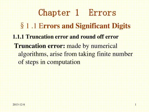
Chapter 1
Errors
§1 .1 Errors and Significant Digits
1.1.1 Truncation error and round off error
Truncation error: made by numerical algorithms, arise from taking finite number of steps in computation
| x * x1 | 0.00173 0.5 102 4 , | x * x2 | 0.00073 0.5 102 4 , | x * x3 | 0.00027 0.5 1025 ,
According to Definition 1.4, x1, x2 and x3 have 4,4 and 5 significant digits respectively.
7
Integration example (cont.)
Choosing a width of 3, we have
x 2 dx ( x 2 )
3 9 x 3
(6 3) ( x 2 )
x 6
(9 6)
(32 )3 (6 2 )3
27 108 135
Actual value is given by
x 3 93 33 2 x dx 3 3 234 3 3
9
9
Truncation error is then
234 135 99
Can you find the truncation error with 4 rectangles? 2013-12-9
If only 3 terms are used,
数值分析(双语版)a12

f [ x, x0 ] = f [ x0 , x1 ] + ( x − x1 ) f [ x, x0 , x1 ]
1 2
n−1 −
…………
f [ x, x0 , ... , xn−1 ] = f [ x0 , ... , xn ] + ( x − xn ) f [ x, x0 , ... , xn ] n−
+ f [ x , x0 , ... , xn ]( x − x0 )...( x − xn−1 )( x − xn )
Nn(x)
ai = f [ x0, …, xi ]
Rn(x)
§2 Newton’s Interpolation
注:
由唯一性可知 Nn(x) ≡ Ln(x), 只是算法不同,故其 , 只是算法不同, 余项也相同, 余项也相同,即 f ( n +1 ) (ξ x ) f [ x , x 0 , ... , x n ]ω k +1 ( x ) = ω k +1 ( x ) ( n + 1) !
§2 牛顿插值
/* Newton’s Interpolation */
Lagrange 插值虽然易算,但若要增加一个节点时, 插值虽然易算,但若要增加一个节点时, 都需重新算过。 全部基函数 li(x) 都需重新算过。
? ? 将 Ln(x) 改写成 a0?+ a1( x − x0 ) + a2 ( x − x0 )(x − x1 ) + ... + a? ( x − x0 )...(x − xn−1 ) 的形式,希望每加一个节点, 的形式,希望每加一个节点, n
1 + (x − x0) × 2 + … … + (x − x0)…(x − xn−1) × −
数值分析英文课件

ˆ ∆y = y − y = 1.4 − 1.41421L ≈ 0.0142
or relative forward error of about 1 percent. Since 1.96 = 1.4 , the absolute backward error is
ˆ ∆x = x − x = 1.96 − 2 = 0.04
Computational error = Truncation error + rounding error
• Propagated (传播) vs. computational error 传播)
– x = exact value, – f = exact function,
ˆ x = approx. value ˆ f = its approximation
Backward vs. forward errors
Suppose we want to compute y = f ( x ) , where f : ℜ → ℜ ˆ but obtain approximate value y
Forward Error:
ˆ ˆ ∆y = y − y = f ( x ) − f ( x )
Example of Ill-Posed Problem
x 1 x 1 x 11 1 + 2 + 3 = 2 3 6 1 1 1 13 x1 + x2 + x3 = 3 4 12 2 1 x1 + 1 x2 + 1 x3 = 47 3 4 5 60
2 significant digits rounding
• Problems that are not well-posed are ill-posed.
数值分析 第9章 常微分方程初值问题数值解法

9 .2 .2 梯形方法/* trapezoid formula */— 显、隐式两种算法的平均 为得到比欧拉法精度高的计算公式, 在等式( 2.4) 右端积分 中若用梯形求积公式近似, 并用yn 代替y ( xn ) , yn+1 代替y ( xn+1 ) ,则得
h yn 1 yn [ f ( xn , yn ) f ( xn 1 , yn 1 )], 2
yn 1 yn f ( xn , yn ), xn 1 xn
即 yn+1 = yn + hf ( xn , yn ) . ( 2 .1)
这就是著名的欧拉( Euler ) 公式.
• 若初值y0 已知, 则依公式( 2.1)可逐步算出
• y1 = y0 + hf ( x0 , y0 ) ,
为了分析迭代过程的收敛性, 将( 2. 7) 式与(2. 8 )式相减, 得
h ( k 1) (k ) yn 1 yn [ f ( x , y ) f ( x , y 1 n 1 n 1 n 1 n 1 )] 2
于是有
| yn 1 y
( k 1) n 1
hL (k ) | | yn 1 yn 1 |, 2
| f ( x, y1 ) f ( x, y2 ) | L | y1 y2 |, y1, y2 R,
定理1 设f在区域D={(x,y)|a≤x ≤b,y∈R}上连续, 关于y满足利普希茨条件,则对任意x0 ∈[a,b], y0 ∈R,常微分方程初值问题(1.1)式和(1.2)式当x ∈[a,b]时存在唯一的连续可微解y(x). 定理2 设f在区域D上连续,且关于y满足利 普希茨条件,设初值问题
1 2 1 2 dy x ydy xdx y x c 2 2 dx y y (0) 2 y2 x2 4
数值分析全册完整课件
似算法的收敛性和数值稳定性; 要有好的计算复杂性,节省时间及存储量; 有数值实验,证明算法有效。
算法基本结构:顺序,分支,循环
算法描述:程序或流程图
常采用的处理方法:
构造性方法 离散化方法 递推化方法 迭代法 近似替代方法 以直代曲法 化整为零的处理方法 外推法
数学基础:
微积分的若干定理: 罗尔定理和微分中值定理; 介值定理及推论; 泰勒公式(一元、二元); 积分中值定理;
设y=f(x)为一元函数,自变量准确值x*,对应函数准确 值y*=f(x*),x误差为e(x),误差限为ε(x),函数近似值 误差e(y),误差限为ε(y)。则(可由Taylor公式推得)
( y) | f '(x) | (x)
r
(
y)
|
xf |f
'(x) (x) |
|
r
(
x)
对于多元函数 z f (x1, x2 ,, xn )
定义1.1 设x*为某一数据的准确值,x为x*的一个近 似值,称e(x)=x-x*(近似值-准确值)为近似值x的绝对 误差,简称误差。
e(x) 可正可负,当e(x) >0时近似值偏大,叫强近似值;当e(x) <0时近似值偏小,叫弱近似值。
由于x*通常无法确定,只能估计其绝对误差值 不超过某整数ε(x),即
设准确值
z* f (x1*, x2*,, xn* )
由多元函数Taylor公式,可得误差估计:
n
(z)
k 1
f xk
(xk )
相对误差限为:
r (z)
n k 1
xk
f xk
r (xk )
z
2. 算术运算的误差估计:
数值分析英文版课件 (6)

12
4.1 Matrix Algebra (III)
The matrix A is denoted as:
1.1 −0.12 3.0 6.2 0.0 0.15 0.6 −4.0 1.3 2.1 8.2 9.3 then a12 = 1.1, or A( 3,2 ) = −4.0 , or ( A )43 = 8.2 .
10
4.1 Matrix Algebra (I)
A matrix is a rectangular array of numbers such as
1.1 −0.12 3.0 6.2 0.0 0.15 , 0.6 −4.0 1.3 9.3 2.1 8.2 3.2 −17 , −4.7 0.11
18
4.1 Matrix Algebra (IX)
Theorem 1 (on equivalent systems):
If one system of equations is obtained from another by a finite sequence elementary operations, then the two systems are equivalent .
3
INDEX
4.0 Introduction 4.1Matrix Algebra 4.2 LU and Cholesky Factorizations
4
INDEX
4.0 Introduction 4.1Matrix Algebra 4.2 LU and Cholesky Factorizations
p
(1 ≤ i ≤ix Algebra (VII)
《数值分析》第二讲插值法PPT课件

1 xn xn2 xnn Vandermonde行列式
即方程组(2)有唯一解 (a0, a1, , an)
所以插值多项式
P (x ) a 0 a 1 x a 2 x 2 a n x n
存在且唯一
第二章:插值
§2.2 Lagrange插值
y
数值分析
1、线性插值
P 即(x)ykx yk k 1 1 x yk k(xxk)
l k ( x k 1 ) 0 ,l k ( x k ) 1 ,l k ( x k 1 ) 0 l k 1 ( x k 1 ) 0 ,l k 1 ( x k ) 0 ,l k 1 ( x k 1 ) 1
lk1(x)(x(k x 1 x xk k))x x ((k 1x k x 1k )1) lk(x)((xx k x xk k 1 1))((x xkxx k k1)1)
第二章:插值
数值分析
3、Lagrange插值多项式
令 L n ( x ) y 0 l 0 ( x ) y 1 l 1 ( x ) y n l n ( x )
其中,基函数
lk (x ) (x ( k x x x 0 ) 0 ) (( x x k x x k k 1 1 ) )x x k ( ( x x k k 1 ) 1 ) (( x x k x n x )n )
因此 P (x ) lk (x )y k lk 1 (x )y k 1
且
P (x k ) y k P (x k 1 ) y k 1
lk(x), lk1(x) 称为一次插值基函数
数值分析
第二章:插值
2、抛物线插值 令
y (xk , yk )
f (x)
lk1(x)(x(k x 1 x xk k))x x ((k 1x k x 1k )1) p( x) (xk1,yk1)
数值分析(英文版)

341
Note that to find f 6 exactly, we only need the value of the function and all its derivatives at some other point, x4 in this case
2013-12-9 13
h2 h3 h4 h5 f x h f x f x h f x f x f x f x 2! 3! 4 5 h2 h3 h4 h5 f 0 h f 0 f 0h f 0 f 0 f 0 f 0 2! 3! 4 5
h2 h3 f x h f x f x h f x f x 2! 3! x4 h 64 2
2013-12-9
12
Example (cont.)
Solution: (cont.) Since the higher order derivatives are zero,
x2 x4 x6 cos(x) 1 2! 4! 6!
x3 x5 x7 sin(x) x 3! 5! 7!
x2 x3 e 1 x 2! 3!
x
2013-12-9
10
General Taylor Series
The general form of the Taylor series is given by f x 2 f x 3 f x h f x f x h h h
22 23 f 4 2 f 4 f 42 f 4 f 4 2! 3! 2 2 23 f 6 125 742 30 6 2! 3!
数值分析课件第二章_非线性方程求根

*
| xn x || ( xn 1 ) ( x ) |
* *
| ( ) || xn 1 x* |
*
| xn x | L | xn1 x | | xn x | L | x0 x |
* n *
lim | xn x | lim L | x0 x | 0
x*即为不动点。
不动点存在的唯一性证明:
设有 x1*≠ x2*, 使得
* 1 * 2 * 1
(x ) x
* 1
* 1
(x ) x
* 2
* 2
* * 则 | x x || ( x ) ( x ) || ( ) || x1 x2 | * 2
其中,ξ介于 x1* 和 x2* 之间。
由于
计法
Ln xn x * x1 x0 1 L
很难估计,采用事后估
| xn x* |
1 | xn 1 xn || xn 1 xn | ,L大误差大。 1 L
不动点迭代法可以求方程的复根和偶数重根。
例 用不同方法求 x 2 3 0 在x=2附近的根。 解: 格式(1)
则对任意x0 [a, b],由xn+1=(xn )得到的迭代序 列{xn }收敛到(x)的不动点x *,并有误差估计:
1 | xn x | | xn 1 xn | 1 L
*
L xn x * x1 x0 1 L
n
证明:
xn ( xn1 ) * * x ( x )
x0
O
x1
x3 x * x2
x0
y ( x)
发散
y ( x)
O
数值分析课件-第02章插值法

数值分析课件-第02章插值法
目录
• 插值法基本概念与原理 • 拉格朗日插值法 • 牛顿插值法 • 分段插值法 • 样条插值法 • 多元函数插值法简介
01 插值法基本概念与原理
插值法定义及作用
插值法定义
插值法是一种数学方法,用于通过已知的一系列数据点,构造一个新的函数, 使得该函数在已知点上取值与给定数据点相符,并可以用来估计未知点的函数 值。
06 多元函数插值法简介
二元函数插值基本概念和方法
插值定义
通过已知离散数据点构造一个连 续函数,使得该函数在已知点处
取值与给定数据相符。
插值方法分类
根据构造插值函数的方式不同, 可分为多项式插值、分段插值、
样条插值等。
二元函数插值
针对二元函数,在平面上给定一 组离散点,构造一个二元函数通 过这些点,并满足一定的光滑性
差商性质分析
分析差商的性质,如差商 的对称性、差商的差分表 示等,以便更好地理解和 应用差商。
差商与导数关系
探讨差商与原函数导数之 间的关系,以及如何利用 差商近似计算导数。
牛顿插值法优缺点比较
构造简单
牛顿插值多项式构造过程相对简 单,易于理解和实现。
差商可重用
对于新增的插值节点,只需计算 新增节点处的差商,原有差商可 重用,节省了计算量。
要求。
多元函数插值方法举例
多项式插值
分段插值
样条插值
利用多项式作为插值函数,通 过已知点构造多项式,使得多 项式在已知点处取值与给定数 据相符。该方法简单直观,但 高阶多项式可能导致Runge现 象。
将整个定义域划分为若干个子 区间,在每个子区间上分别构 造插值函数。该方法可以避免 高阶多项式插值的Runge现象 ,但可能导致分段点处的不连 续性。
数值分析全套课件

Ln n si n
ˆ L2n (4L2n Ln ) / 3
n L error 192 3.1414524 1.4e-004 384 3.1415576 3.5e-005 3.1415926 4.6e-010
3/16
通信卫星覆盖地球面积
将地球考虑成一 个球体, 设R为地 球半径,h为卫星 高度,D为覆盖面 在切痕平面上的 投影(积分区域)
( x1 x2 ) | x1 | ( x2 ) | x2 | ( x1 )
15/16
例3.二次方程 x2 – 16 x + 1 = 0, 取
求 x1 8 63 使具有4位有效数
63 7.937
解:直接计算 x1≈8 – 7.937 = 0.063
( x1 ) (8) (7.937) 0.0005
5/16
误差的有关概念
假设某一数据的准确值为 x*,其近似值 为 x,则称
e(x)= x - x*
为 x 的绝对误差 而称
e( x) x x er ( x ) , x x
*
( x 0)
为 x 的相对误差
6/16
如果存在一个适当小的正数ε
,使得
e( x) x x
计算出的x1 具有两位有效数
1 0.062747 修改算法 x1 8 63 15.937 4位有效数 (15.937) 0.0005 ( x1 ) 0.000005 2 2 (15.937) (15.937)
16/16
1
参考文献
[1]李庆扬 关治 白峰杉, 数值计算原理(清华) [2]蔡大用 白峰杉, 现代科学计算 [3]蔡大用, 数值分析与实验学习指导 [4]孙志忠,计算方法典型例题分析 [5]车刚明等, 数值分析典型题解析(西北工大) [6]David Kincaid,数值分析(第三版) [7] John H. Mathews,数值方法(MATLAB版)
数值分析英文版课件1

则有
B
Qn (
f
) Qn (
f
)
max 0kn
f ( xk )
f ( xk )
( x )dx
a
21
8.5.2 Gauss 型求积公式的稳定性与收 敛性(3)
关于Gauss 求积公式
b
(
a
x
)
f
(
x
)dx
n
k 0
Ak( n
)
f
(
xk( n
)
)
的收敛性有如下定理,上式中特别标出了求积系 数与节点和 n 有关。
2
8.5 Gauss 型求积公式(3)
对于给定的节点数目 n+1,适当调整其位置,是 否会提高求积公式的代数精度?
例8.5.1 对于求积公式
1
f ( x )dx A0 f ( x0 ) A1 f ( x1 )
1
试确定其节点 x0, x1 及求积系数 A0, A1,使其代 数精度尽可能高
22
8.5.2 Gauss 型求积公式的稳定性与收 敛性(4)
定理8.5.5
设 f C [a, b]
令 Qn ( f ) n Ak( n ) f ( xk( n ) ) k 0
则有
b
lim
n
Qn
(
f
)
( x ) f ( x )dx
a
23
今日课题
第八章 数值积分与数值微分
8.1 Newton-Cotes求积公式 8.2 复合求积公式 8.5Gauss型求积公式
那么相应的正交多项式为 Legendre多项式 Pn(x)
P0 ( x ) 1
Pn (
数值分析英文版课件 3

6
3的根x*的近似解序列。
1 bn an n1 (b a) 2
而xn是[an,bn]的中点,所以有
1 1 | xn x | (bn an ) n (b a) 2 2
*
n
lim xn x*
7
3.2.1 二分法 (3)
为求解方程 f(x)=0 的根 x*,假设
有一个近似值 xk ≈ x* f ’’存在且连续
因 f (x*)=0, 则:
'' f ( ) ' f ( x ) f ( xk ) f ( xk )( x xk ) ( x x k )2 2 若 f ' (x*) ≠0,
今日主题
第三章:非线性方程的数值解法
3.1 引言 3.2 二分法和试位法 3.3 不动点迭代法 3.4 迭代加速收敛的方法 3.5 Newton 迭代法
1
今日主题
第三章:非线性方程的数值解法
3.1 引言 3.2 二分法和试位法 3.3 不动点迭代法 3.4 迭代加速收敛的方法 3.5 Newton 迭代法
( x x* ) g ( x ) m ( x) mg ( x) ( x x* ) g '( x)
所以x*是方程 m(x)=0 的单根
33
3.5.2 Newton 法的重根情形 (5)
应用Newton法,迭代函数为:
m ( x) f ( x) f '( x) ( x) x x ' m '( x) [ f ( x)]2 f ( x) f ''( x)
- 1、下载文档前请自行甄别文档内容的完整性,平台不提供额外的编辑、内容补充、找答案等附加服务。
- 2、"仅部分预览"的文档,不可在线预览部分如存在完整性等问题,可反馈申请退款(可完整预览的文档不适用该条件!)。
- 3、如文档侵犯您的权益,请联系客服反馈,我们会尽快为您处理(人工客服工作时间:9:00-18:30)。
2.2 GEM
Denote Ax=b as A(1)x=b(1),where A(1) and b(1) with ( entries aij1) and bi(1) , respectively. The goal in the first elimination process is changing the n-1 (1 entries below a11) into 0. We denote the resulting system by A(2)x=b(2).
1 2 3 1 r2 r2 2 r1 1 2 3 1 0 3 1 4 A : b 2 7 5 6 r3 r3 r1 1 4 9 3 0 2 6 4
2013-12-9 4
1 2 3 1 2 r3 r3 r2 3 0 3 1 4 20 20 0 0 3 3
7
Like the first elimination process, the goal of k-th ( is eliminating the entries below ak kk) . The operations , in detail are as follows: ( aikk ) i k 1, , n (multipliers) lik ( k ) akk ( k 1) ( ( aij aijk ) lik akjk ) i , j k 1, k 2, , n ( k 1) ( bi bi( k ) lik bk k ) i k 1, k 2, , n (k akk ) If ≠0,(k=1,2,,n-1), the process can continue. Finally, we obtain the following matrix (1) (1) a11 a12 a1(1) b1(1) n (2) (2) (2) a22 a2 n b2 (n) (n) A b (n) (n) ann bn
x1 2 x 2 3 x3 1 3 x 2 x3 4 2 x 2 6 x 3 4
3
The 2nd step: the second equation times by -2/3and adds to the third equation, we have x1 2 x 2 3 x3 1 3 x 2 x3 4 20 20 x3 3 3 The 3rd step: solve the linear system by backward substituting, we have x*=(2,1,-1)T The above process can be described by matrix form as
(2) an 2
a1(1) b1(1) n (2) ( a2 n b2 2) A(2) b (2) (2) (2) ann bn
2013-12-9
6
(k akk ) ≠0),we have After k-1th eliminations(suppose
2013-12-9 11
§3 Gaussian Elimination with Pivoting
In the previous section, the GEM perhaps get a (k solution with a great error when | akk ) | <<1,because multipliers perhaps are very huge and the computation error is amplified largely.
( aiii ) 2backward substitution ( ≠0)
( bnn ) xn (n) a nn n (i ) ( bi a iji ) x j j i 1 xi ( a iii )
(i=n-1,n-2,,1)
10
2013-12-9
2013-12-9 5
(1) a11 (1) (1) (1) a21 A b (1) an1 (1) a11 0 0 (1) a12 (2) a22
(1) a12 (1) a22
(1) an 2
a1(1) b1(1) n (1) (1) ri ri li 1 r1 a2 n b2 ( i 2,3,, n ) (1) (1) ann bn
xj
Dj D
j 1, 2, , n
where D=det(A), and Dj is the determinant of the matrix obtained by substituting j-th column of A with the right hand side b. There exist two classes of methods for solving linear systems: direct methods and iterative methods。
( a11) k ( a22 ) k
A
(k )
:b
(k )
(k akk )
(k ank )
2013-12-9
( a11) b1(1) n ( 2) ( 2) a2 n b2 (k ) (k ) akn bk (k ) (k ) ann bn
2013-12-9
2
§2 Gaussian Elimination Method
2.1 The Idea of GEM Eg.2.1 Solve the following linear system of equations
x1 2 x 2 3 x3 1 2 x1 7 x 2 5 3 6 x 4 x 9 x 3 2 3 1
Eg. 2.2 Solve the following linear system of equation using 3 significant digits.
0.50 x1 1.1x2 3.1x3 6.0 2.0 x1 4.5 x2 0.36 x3 0.020 5.0 x 0.96 x 6.5 x 0.96 1 2 3
( bn n ) xn ( n ) ann n ( bi( i ) aiji ) x j j i 1 xi ( aiii )
(i=n-1,n-2,,1)
In a word, we can get the algorithm of GEM: step 1elimination process ( ①set aij1) aij , bi(1) bi (i,j=1,2,…,n)
2013-12-9 8
Because the matrix A(n) is an upper triangular matrix, the linear system of equations is changed (n into a triangular system of equations. If ann) ≠0,we obtain the solution
2013-12-9 12
Solution. ( The accurate solution x*=(-2.6, 1, 2)T.) Method I: 0.50 1.1 2.0 4.5 5.0 0.96 normal GEM 3.1 6.0 0.500 0.36 0.020 0 6.5 0.96 0
Chapter 2 Direct Methods for Solving Linear Systems
§0 Introduction
Consider the system:
a11 x1 a12 x2 a1n xn b1 a x a x a x b 21 1 22 2 2n n 2 an1 x1 an 2 x2 ann xn bn
2.3 A Condition on GEM From the previous algorithm, we need assume the (k entry akk ) ≠0 in the k-th elimination process. In (k order to finish the GEM, the condition akk ) ≠ 0 for all k. But we hope decide only according to A whether the GEM can finish or not. So, we have the theorem: Theorem 2.1 GEM can continue iff all principal minor determinants in order of A don’t equal 0. To compute elimination 2(n-1)n(n+1)/6 + n(n-1) flops are required, plus n2 flops to backward substitution. Therefore, about (n3/3 + 2n2 ) flops are needed to solve the linear system using GEM.
The 1st step, the first equation times by -2 and adds to the second equation, and the first equation times by -1 and adds to the third equation.