NUMERICAL METHODS Chapter10

合集下载

Chapter 3 Descriptive statistics(Numerical methods)

Chapter 3 Descriptirth noticing (1) Weight（权数）: The number to measure the importance (weights) of variables→ “f or f/∑f” ∑ [Example] During the “Oct. 1st”, 10 students go to different tourist site: Mt. Huang→5 persons, Mt. Wuyi→2 , Mt. Tai→2 , Mt. Laofu→1.
Total age 15 + 16 + 16 + L + 18 170 x= = = = 17 Number of persons 1+1+1+L+1 10
x1 + x 2 + x 3 + L + x n Σx ∴x = = = E ( x) 1+1+1+L+1 n Σx （1）Simple arithmentic mean：x = n
Difficulties
1. Mean； Mean； 2. Variance and standard deviation。 deviation。
Chapter 3 Descriptive statistics
STAT
Section 1 Central tendency and tendency of dispersion 1. Concepts tendency（集中趋势） 1） Central tendency（集中趋势）: The closer to middle the variable gets, the larger the frequency is. The reverse is also true. 2） Tendency of dispersion（离中趋势）: The tendency of dispersion（离中趋势） deviating and dispersed at the two ends.

宏观经济学(第十版)N格里高利曼昆-2024鲜版

通货膨胀的类型
根据通货膨胀的成因和特点，可以将通货膨胀分为需求拉上型通货膨胀、成本推进型通货膨胀、输入型通货膨胀和结构性通货膨胀等类型。
2024/3/28
通货膨胀的原因
通货膨胀的原因较为复杂，可能包括总需求过度、成本上升、国际收支失衡、货币供应过多等因素。
16
经济增长的定义、影响因素与政策
2024/3/28
货币政策的定义、目标与工具
价格稳定
通过控制通货膨胀率，保持物价稳定，避免经济波动。
经济增长
通过调节利率和信贷条件，促进投资和消费，推动经济增长。
2024/3/28
32
货币政策的定义、目标与工具
2024/3/28
• 汇率稳定：在开放经济中，通过干预外汇市场，维护本国货币汇率的稳定。
33
货币政策的定义、目标与工具
宏观经济学(第十版 )N格里高利曼昆
2024/3/28
1
目录
2024/3/28
• 引言 • 国民收入核算与宏观经济指标 • 失业、通货膨胀与经济增长
2
目录
2024/3/28
• 货币、利率与金融市场 • 总需求与总供给模型 • 财政政策与货币政策 • 开放经济下的宏观经济政策
3
引言
01
2024/3/28
失业的类型
根据失业的原因和性质，可以将失业分为摩擦性失业、结构性失业、周期性失业和自然失业等类型。
失业的原因
失业的原因多种多样，包括经济周期波动、产业结构调整、技术进步、劳动力市场制度不完善、信息不对称等。
2024/3/28
15
通货膨胀的定义、类型与原因
通货膨胀的定义
通货膨胀是指一般物价水平持续上涨的现象，即货币的购买力不断下降的过程。

数值分析第一课

Introduction
What is Numerical Analysis?
What is numerical analysis?
Numerical analysis is the main part of Computional Methods. It involves the study, development, and analysis of algorithms for obtaining numerical solutions to various mathematical problems.
8
12
As a consequence, this machine number precisely represents the decimal number
( 1) 2
0
1027 1023
(1 f ) 27.56640625
Underflow
The smallest positive number that can be represented has s 0, c 1, f 0
Numerical Analysis
yangyang@
Textbook (not necessarily to have)
Numerical Analysis (Seventh Edition) 数值分析（第七版影印版） Richard L. Burden & J. Douglas Faires （高等教育出版社）
Contents of the text
Chapter 2: Solutions of Equations in One Variable (非线性方程的数值解法)
Chapter 10: Numerical Solutions of Nonlinear Systems of Equations (非线性方程组的数值解)

数值方法(第2版)答案

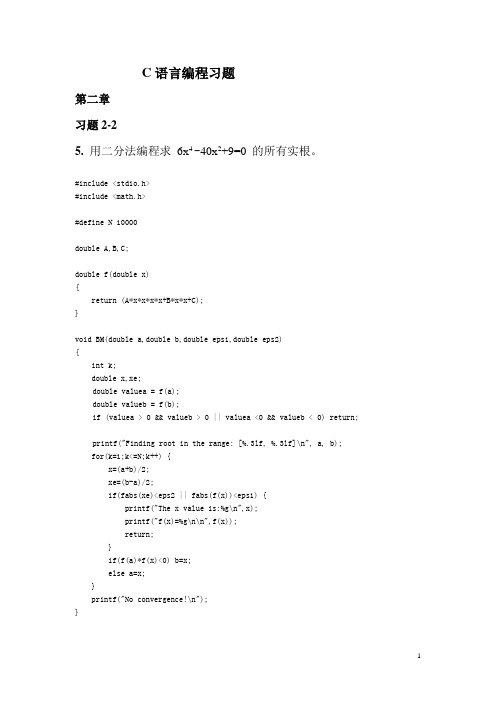
C语言编程习题第二章习题2-25.用二分法编程求6x4 -40x2+9=0 的所有实根。

#include <stdio.h>#include <math.h>#define N 10000double A,B,C;double f(double x){return (A*x*x*x*x+B*x*x+C);}void BM(double a,double b,double eps1,double eps2){int k;double x,xe;double valuea = f(a);double valueb = f(b);if (valuea > 0 && valueb > 0 || valuea <0 && valueb < 0) return;printf("Finding root in the range: [%.3lf, %.3lf]\n", a, b);for(k=1;k<=N;k++) {x=(a+b)/2;xe=(b-a)/2;if(fabs(xe)<eps2 || fabs(f(x))<eps1) {printf("The x value is:%g\n",x);printf("f(x)=%g\n\n",f(x));return;}if(f(a)*f(x)<0) b=x;else a=x;}printf("No convergence!\n");}int main(){double a,b,eps1,eps2,step,start;printf("Please input A,B,C:\n");scanf("%lf %lf %lf",&A,&B,&C);printf("Please input a,b, step, eps1,eps2:\n");scanf("%lf %lf %lf %lf %lf",&a,&b,&step,&eps1,&eps2);for (start=a; (start+step) <= b; start += step) { double left = start;double right = start + step;BM(left, right, eps1, eps2);}return 0;}运行：Please input A,B,C:6 -40 9Please input a,b, step, eps1,eps2:-10 10 1 1e-5 1e-5Finding root in the range: [-3.000, -2.000]The x value is:-2.53643f(x)=-0.00124902Finding root in the range: [-1.000, 0.000]The x value is:-0.482857f(x)=0.00012967Finding root in the range: [0.000, 1.000]The x value is:0.482857f(x)=0.00012967Finding root in the range: [2.000, 3.000]The x value is:2.53643f(x)=-0.00124902有时若把判别语句if(fabs(xe)<eps2 || fabs(f(x))<eps1)改为if(fabs(xe)<eps2 && fabs(f(x))<eps1)会提高精度，对同一题运行结果：Finding root in the range: [-3.000, -2.000]The x value is:-2.53644f(x)=-4.26496e-007Finding root in the range: [-1.000, 0.000]The x value is:-0.482861f(x)=-7.3797e-006Finding root in the range: [0.000, 1.000]The x value is:0.482861f(x)=-7.3797e-006Finding root in the range: [2.000, 3.000]The x value is:2.53644f(x)=-4.26496e-007习题2-35. 请用埃特金方法编程求出x=tgx在4.5（弧度）附近的根。

NumericalIntegration

∫ ∑ ∫ ∑ ∫ b F (r)dr
a
=
n i =1
⎡ ⎢⎣
b a
li
(r
)dr
⎤ ⎥⎦
Fi
+
∞ j=0
⎡ ⎢⎣
b
r
a
j P(r)dr⎥⎦⎤β j
∫ ∑ ∫ ∑ ∫ ( ) ( ) b F (r)dr
a
=
n⎡ i=1 ⎢⎣
b
a li
r
dr
⎤ ⎥⎦
Fi
+
n−1 j=0
⎡ ⎢⎣
br jP
a
r
dr⎥⎦⎤β j
x
N=1, F=12, Error= -5.26%
x
N=2, F=12.5, Error= -1.32%
Numerical Integration
Integration using numerical methods:
Numerical integration
y
y = x2 + 6
y
y = x2 + 6
Numerical integration
Scheme 2:
Same as Scheme 1, except that we choose a linear function in each section to approximate the variation of f (x). This linear function takes the same value and slope of f (x) at the mid-point of that section.
Interpolation using a polynomial

《统计学习方法》第2版课件第10章隐马尔科夫模型-2021年必备

于是求得最优路径，即最优状态序列：
人脸检测
人人脸脸检图测像预处理
光线补偿
中值滤波归一化处理
人脸识别
HMM训练步骤：对每个人脸建立一个 HMM
1、人脸特征向量提取 2、建立公用的HMM模型 3、HMM初始参数确定 4、初始模型参数训练，主要是运用Viterbi
算法训练均匀分割得到参数，求得最佳分割点，然后重新计算模型初始参数，直到模型收敛为止。
对固定的状态序列I，观测序列O的概率：
O和I同时出现的联合概率为：
对率所：有可能的状态序列I求和，得到观测O的概复杂度
前向算法
前向概率定义：给定隐马尔科夫模型λ，定义到时刻
t部分观测序列为：
，且状态为qi的概率为
前向概率，记作：
初值：递推：
前向算法
因为：
所以：
递推：
复杂度
前向算法
两个基本假设
齐次马尔科夫性假设，隐马尔可分链t的状态只和t-1状态有关：
观测独立性假设，观测只和当前时刻状态有关；
例：盒子和球模型
盒子： 1 红球： 5 白球： 5
234 368 742
转移规则：
盒子1 下一个盒子2 盒子2或3 下一个 0.4 左，0.6右盒子4 下一个 0.5 自身，0.5盒子3
一些概率和期望值的计算
一些概率和期望值的计算
一些概率和期望值的计算
学习算法
监督学习方法：
假设训练数据是包括观测序列O和对应的状态序列I
可以利用极大似然估计法来估计隐马尔可夫模型参数。
非监督学习方法：
假设训练数据只有S个长度为T的观测序 {O1,O2,…Os},
采用Baum-Welch算法

Numerical Descriptive Techniques

Sample mean
x=
n n x ∑i=11x i i i=
Population mean
∑N 1 x i i= µ= N
Population size
n n
Sample size
5
Hale Waihona Puke The arithmetic mean
The Arithmetic Mean
• Example 4.1
The reported time on the Internet of 10 adults are 0, 7, 12, 5, 33, 14, 8, 0, 9, 22 hours. Find the mean time on the Internet.
12
The Geometric Mean
The Geometric Mean
For the given series of rate of returns the nth period return is calculated by: If the rate of return was Rg in every period, the nth period return would be calculated by: n (1 + R1 )(1 + R 2 )...(1 + R n ) = (1 + R g )
• All observation except “0” occur once. There are two “0”. Thus, the mode is zero. • Is this a good measure of central location? • The value “0” does not reside at the center of this set (compare with the mean = 11.0 and the mode = 8.5).

NUMERICAL METHODS Chapter08

CHAPTER 8
NUMERICAL ORDINARY DIFFERENTIAL EQUATIONS
(ODE) This chapter is about solving for a function of time y(t) when its time-derivative is given, namely,
yi+1
k = f (ti, yi)
y(t) yi
t
ti h ti+1
A. Difference equation When propagating from i to i+1, the propagation slope is simply approximated as:
k= dy = f (ti , yi ) dt ti
yi +1 + δyi +1 = yi + δyi + f (ti , yi ) h + ∂f (ti , yi ) δyi h ∂y
δyi +1 = δyi +
∂f (ti , yi ) δyi h ∂y δyi +1 ∂f (ti , yi ) h =1+ δyi ∂y
For the calculation to be stable, the round-off error has to diminish as i increases. The stability condition is: ∂f 1+ h <1 ∂y ∂f ∴0 < − h < 2 . ∂y Therefore, the method is only conditionally stable.
dy = f (e derivative depends on time t and the instantaneous value of y itself. The function f can be a complicated function that requires numerical treatments. If f does not depend on y, the numerical integrations of Chapter 7 are applicable. Otherwise, we need to deal with the problem using tools of the current chapter. The problem of Eq. (*) is called a first-order ordinary differential equation (ODE). It is of first order because only the first derivative is involved. It is regarded as “ordinary” because the differentiation is only about a single variable t. It is clear that the initial value y(0) at t = 0 has to be given. The problem is an example of initial value problems (IVP). Numerical ODE solution with increasing accuracies are presented in this chapter. They are Euler’s method, Heun’s method and Runge-Kutta 4th order method. While these methods use equal step size, Matlab has some built-in functions with adaptive step sizes. Example of using ode functions will be discussed.

数值方法-Numerical Methods

• Radial basis function splines in multiple dimensions.
• LU and QR factorisation and applications.
• Norms and condition numbers. Jacobi method.
• Fixed point iteration, Newton's method.
Syllabus ofMathematicsand Applied Mathematicsat Haide College
Numerical Methods
Description
To explore complex systems, physicists, engineers, financiers and mathematicians require computational methods since mathematical models are only rarely solvable algebraically. Numerical methods, based upon sound computational mathematics, are the basic algorithms underpinning computer predictions in modern systems science. Such methods include techniques for simple optimisation, interpolation from the known to the unknown, linear algebra underlying systems of equations, ordinary differential equations to simulate systems, and stochastic simulation under random influences.

Numerical Methods

Bisection method…
• This method converges to any pre-specified tolerance when a single root exists on a continuous function • Example Exercise: write a function that finds the square root of any positive number that does not require programmer to specify estimates
Finding roots, continued
• Transcendental equations: involving geometric functions (sin, cos), log, exp. These equations cannot be reduced to solution of a polynomial. • Convergence: we might imagine a “reasonable” procedure for finding solutions, but can we guarantee it terminates?
Problem with Bisection
• Although it is guaranteed to converge under its assumptions, • Although we can predict in advance the number of iterations required for desired accuracy (b - a)/2n <e -> n > log( (b - a ) / e ) • Too slow! Computer Graphics uses square roots to compute distances, can’t spend 15-30 iterations on every one! • We want more like 1 or 2, equivalent to ordinary math operation.

传热学专业英语词汇

Chapter 1 Thermodynamics and Heat Transfer 主要内容1.Concepts:heat (thermal energy)、heat transfer、thermodynamics、total amount of heat transfer、heat transfer rate、heat flux、conduction、convection、radiation2.Equations:1) The first law of thermodynamics (conservation of energy principle)2) Heat balance equation: a) closed system; b) open system (steady-flow)3) Fourier’s law of heat conduction4) Newton’s law of cooling5) Stefan-Boltzmann law主要专业词汇heat transfer 传热、热传递、传热学thermodynamics热力学caloric 热素specific heat 比热mass flow rate 质量流率latent heat 潜热sensible heat 显热heat flux热流密度heat transfer rate热流量total amount of heat transfer总热量conduction导热convection对流radiation辐射thermal conductivity 热导率thermal diffusivity 热扩散率convection/combined heat transfer coefficient 对流/综合换热系数emissivity 发射率absorptivity 吸收率simultaneous heat transfer 复合换热Chapter 2 Heat Conduction Equation主要内容1.Concepts:temperature field、temperature gradient、heat generation、initial condition、boundary condition、steady\transient heat transfer、uniform\nonuniform temperature distribution2.Equations:1) Fourier’s law of heat conduction (§2-1)2) Heat conduction equation (inrectangular\cylindrical\spherical coordinates) (§2-2、§2-3)3) Boundary conditions: (§2-4)a)Specified temperature B. C.b) Specified heat flux B. C. [special case(dt/dx=0):insulation、thermal symmetry];c) Convection B.C.d) Radiation B.C.e) Interface B.C.4) Average thermal conductivity k ave(§2-7)5) Solution of one-dimensional, steady heat conduction inplane walls、cylinders and spheres (k =const)：a) no heat generation, specified B.C.: T(x) or T(r) (§2-5)Q(x) or Q(r), Q=constb) with heat generation, Specified B.C. or Convection B.C. : (§2-6)∆T max=T o-T s= gs2/2nk ; q(x)=gx/n; T s=T + gs/nh characteristic length S, shape factor n:plane walls —s = L (half thickness), n = 1cylinders ——s =r o, n = 2spheres ——s =r o, n =33.Methods: Solve a heat transfer problem1) Mathematical formulation (differential equation & B.C.)2) General solution of equation3) Application of B.C.s4) Unique solution of the problem主要专业词汇temperature field\distribution温度场\分布temperature gradient温度梯度heat generation热生成(热源)initial\boundary condition初始\边界条件transient heat transfer瞬态(非稳态)传热isothermal surface 等温面Heat conduction differential equation 导热微分方程trial and error method试算法iterate迭代convergence 收敛Chapter 3 Steady Heat Conduction主要内容1.Concepts:multilayer\composite wall overall heat transfer coefficient Uthermal resistance R t thermal contact resistance R c critical radius of insulation R crfin efficiency fin effectiveness2.Equations:✓Multiplayer plane wall、cylinders and spheres:✓Fin: fin equation——refer to the attachment.1) Uniform cross-section: refer to the attachment.2) Varying cross-section: refer to the attachment.主要专业词汇thermal resistance热阻parallel 并联in series串联thermal contact resistance 接触热阻composite wall 复合壁面thermal grease 热脂cross-section 横截面temperature execess 过余温度hyperbolic 双曲线的exponent 指数fin 肋(翅)片fin base 肋基fin tip 肋端fin efficiency 肋效率fin effectiveness 肋片有效度Chapter 4 Transient Heat Conduction主要内容1.Concepts:lumped system analysis characteristic length (L c=V/A)Biot number (Bi=hL c /k) Fourier number ( τ = at/L)2.Equations:●Bi≤0, lumped system analysis (§4-1)●Bi>0, Heisler/Grober charts OR analytical expressions1-D：a) infinite large plane walls, long cylinders and spheres (§4-2)b) semi-infinite solids (§4-3)multidimensional: product solution (§4-4)主要专业词汇lumped system analysis 集总参数法characteristic length 特征长度（尺寸）dimension 量纲nondimensionalize 无量纲化dimensionless quantity 无量纲量semi-infinite solid 半无限大固体complementary error function 误差余函数series 级数production solution 乘积解Chapter 5 Numerical Methods in Heat Conduction主要内容1.Concepts:control volume (energy balance) method、finite difference method、discretization、node、space step、time step、mesh Biot number、mesh Fourier number、mirror image concept、explicit/implicit method、stability criterion (primary coefficients ≥0)Numerical error: 1) discretization/truncation error; 2) round-off error2.Methods:Numerical solution:1) Discretization in space and time (∆x, ∆t);2) Build all nodes’finite difference formulations (including interior and boundary nodes);i.Finite difference methodii.Energy balance method (i.e.Control Volume method)3) Solution of nodal difference eqs. of heat conduction;i.Direct method: Gaussian Eliminationii.Iterative method: Gauss-Seidel iteration主要专业词汇control volume 控制容积finite difference有限差分Taylor series expression泰勒级数展开式mirror image concept 镜像法Elimination method 消元法direct/iterative method 直接/迭代方法explicit/implicit method 显式/隐式格式stability criterion 稳定性条件primary coefficients 主系数unconditionally 无条件地algebraic eq. 代数方程discretization/truncation error 离散/截断误差round-off error 舍入误差Chapter 6、7 Forced Convection and NaturalConvection主要内容1.Concepts:Nu、Re、Gr、PrForce/natural convection、external/internal flow、velocity/thermal boundary layerflow regimes、laminar/turbulent flowhydrodynamic/thermal entry region、fully developed regionCritical Reynolds Number (Re c)、hydraulic diameter (D h)、film temperature (T f)、bulk mean fluid temperature (T b)logarithmic mean temperature difference ( T ln)volume expansion coefficient (β= 1/T)effective thermal conductivity (K eff = K Nu)2.Equations:Drag force ：F D = C f AρV2/2Heat transfer rate：Q = hA(T s-T )3．Typical Convection Phenomena:1) Forced convection：external flow——flow over flat plates (§6-4)——flow across cylinders and spheres (§6-5)internal flow——flow in tubes (§6-6)2) Natural convection：flow over surfaces (§7-2)flow inside enclosures (§7-3)主要专业词汇Force/natural convection 自然/强制对流laminar/turbulent flow 层/湍流boundary layer 边界层laminar sublayer 层流底层buffer layer 缓冲层transition region 过渡区flow regimes 流态inertia/viscous force 惯性/粘性力shear stress 剪切应力friction/drag coefficient 摩擦/阻力系数friction factor 摩擦因子dynamic/kinematic viscous 动力/运动粘度wake 尾流stagnation point 滞止点flow separation 流体分离vortex 漩涡rotational motion 环流velocity fluctuation 速度脉动hydrodynamic 水动力学的hydraulic diameter 水力直径fully developed region 充分发展段volume flow rate 体积流量arithmetic/logarithmic mean temperature difference 算术/对数平均温差volume expansion coefficient 体积膨胀系数interferometer 干涉仪asymptotic渐近线的effective thermal conductivity 有效热导率analogical method 类比法integral approach 积分近似法order of magnitude analysis 数量级分析法similarity principle 相似原理Chapter 9 Radiation Heat Transfer主要内容1.Concepts:black body、gray body、diffuse surface、emissive power (E)emissivity (ε)、absorptivity (α)、reflectivity (ρ)、transmissivity (τ) irradiation(G)、radiosity(J)、reradiating(adiabatic) surfaceview factor (F ij)、radiation network、space resistance、surface resistance radiation shieldgas radiation、transparent medium to radiation、absorbing and transmitting mediumws:Blackbody：(1) Plank’s law(2) Stefan-Boltzmann’s law(3) Wien’s displacement lawGraybody：(4) Kirchhoff’s lawActual body：E (T) = εE b(T) = εσT4W/m2Gas：(5) Beer’s law3．Calculation:1) View factor：reciprocity/summation/superposition/symmetry Rulecrossed-strings method2) Radiation heat transfer：Radiation networkOpen system：between two surface (e.g. two large parallel plates) Enclosure：2-surface enclosure；3-surface enclosureRadiation shield主要专业词汇thermal radiation热辐射、quantum theory量子理论、index of refraction 折射系数electromagnetic wave/spectrum 电磁波/波谱、ultraviolet (UV) rays紫外线、infrared (IR) rays 红外线absorptivity 吸收率、reflectivity 反射率、transmissivity 透射率、emissivity (ε) 发射率(黑度)、specular/diffuse reflection 镜反射/漫反射irradiation (incident radiation) 投入辐射、radiosity 有效辐射spectral/directional/total emissive power单色/定向/总辐射力fraction of radiation energy 辐射能量份额(辐射比)、blackbody radiation function 黑体辐射函数view factor 辐射角系数、crossed-strings method交叉线法、reciprocity/summation/superposition/symmetry Rule相互/完整/和分/对称性net radiation heat transfer 净辐射热流量radiation network 辐射网络图、space/surface radiation resistance 空间/表面辐射热阻、reradiating surface重辐射面、adiabatic 绝热的radiation shield遮热板transparent medium to radiation辐射透热体、absorbing and transmitting medium吸收-透过性介质Chapter 10 Heat Exchangers主要内容1.Concepts:heat exchanger type---- double-pipe、compact、shell-and-tube、plate-and-frame、regenerative heat exchangerparallel/counter/cross/multipass flowoverall heat transfer coefficient (U) fouling factor (R f)heat capacity rate capacity rationlog mean temperature difference (ΔT lm)heat transfer effectiveness (ε)number of transfer units (NTU)2.Equations:1) heat balance eq.: Q = C h (T h,in - T h,out)=C c(T c,out - T c,in)2) heat transfer eq.: Q = UAΔT lm( LMTD method)or Q = εQ max = εC min (T h,in ？C T c,in) ( ε-NTU method) 3．Methods:1) LMTD Method：select a heat exchangerKnown: C h、C c、3‘T’Predict: 1‘T’、Q、A2) ε-NTU Method：evaluate the performance of a specified heat exchangerKnown: C h、C c、UA、T h,in、T c,inPredict: Q、T h,out、T c,out主要专业词汇double-pipe/compact/shell-and-tube/plate-and-frame/regenerative heat exchanger套管式/紧凑式/壳管式/板式/蓄热（再生）式换热器parallel/counter/cross/multipass flow 顺流/逆流/叉流/多程流area density 面积密度tube/shell pass 管程/壳程static/dynamic type 静/动态型baffle 挡板header 封头nozzle管嘴guide bar 导向杆porthole 孔口gasket 垫圈lateral 侧面的/横向的fouling factor 污垢因子heat capacity rate 水当量heat transfer effectiveness (ε) 传热有效度number of transfer units (NTU) 传热单元数。

numerical method

numerical method
数值方法是一种求解运筹学问题的方法，它利用数学分析和计算机程序来帮助解决复杂的运筹学问题。

它主要包括几乎所有广义上的数学计算，从微积分，积分变换，几何处理，函数逼近到求解线性和非线性方程组，优化，积分，求根，图形处理，随机数生成器等。

它可以用于处理经典的数学问题，例如求解微分方程组，求解计算机图形学中的三维物体的外部表面，以及求解矩阵和向量运算中的线性方程组。

它还可以用于解决一些更为复杂的问题，例如结构优化，快速傅里叶变换（FFT），计算流体力学，计算熵，最优化等等。

有关于数学归纳法的英文文献

有关于数学归纳法的英文文献Mathematical induction is a powerful and fundamental proof technique used in mathematics to establish the truth of statements or propositions that involve natural numbers. It is a deductive reasoning method that allows one to prove that a given statement is true for all natural numbers, starting from a base case and then showing that if the statement is true for a particular natural number, then it is also true for the next natural number.The essence of mathematical induction lies in the fact that the natural numbers form an ordered set with a well-defined starting point, the number 1, and a clear successor relationship, where each natural number has a unique next number. This structure allows us to build up proofs by starting with the base case and then demonstrating that the statement holds for the next number, and so on, until we can conclude that the statement is true for all natural numbers.The general structure of a mathematical induction proof consists of two main steps:1. Base case: Establish that the statement is true for the first natural number, typically 1.2. Inductive step: Assume that the statement is true for a particular natural number k, and then show that it is also true for the next natural number, k+1.Once these two steps are completed, the principle of mathematical induction allows us to conclude that the statement is true for all natural numbers.One of the key advantages of mathematical induction is its ability to handle statements that involve an infinite number of cases, such as those related to sequences, series, or properties of natural numbers. By proving the statement for the base case and then showing that it holds for the next number, we can establish the truth of the statement for all natural numbers, even though there are infinitely many of them.Mathematical induction has a wide range of applications in various branches of mathematics, including number theory, combinatorics, algorithm analysis, and even in some areas of computer science and physics. It is a fundamental tool for proving the correctness of algorithms, establishing properties of recursive data structures, and solving problems that involve the manipulation of natural numbers.One classic example of the application of mathematical induction is the proof of the formula for the sum of the first n positive integers, which states that the sum of the first n positive integers is equal to n(n+1)/2. To prove this formula using induction, we first establish the base case by showing that the statement is true for n=1, as 1(1+1)/2 = 1. Then, we assume that the statement is true for some natural number k, and we show that it is also true for the next natural number, k+1, by using the following steps:Assume the statement is true for n=k:Sum of the first k positive integers = k(k+1)/2Now, consider the sum of the first k+1 positive integers:Sum of the first k+1 positive integers = 1 + 2 + 3 + ... + k + (k+1)= (k(k+1)/2) + (k+1)= (k(k+1) + 2(k+1))/2= (k^2 + 3k + 2)/2= (k+1)(k+2)/2Therefore, the statement is also true for n=k+1. By the principle of mathematical induction, we can conclude that the formula for the sum of the first n positive integers is true for all natural numbers n.Another important application of mathematical induction is in thefield of algorithm analysis, where it is used to prove the correctness and runtime complexity of algorithms. For example, when analyzing the time complexity of a recursive algorithm, we can use induction to show that the algorithm's running time grows in a certain way as the input size increases.Consider the classic Fibonacci sequence, where each number in the sequence is the sum of the two preceding numbers, starting with 0 and 1. We can use mathematical induction to prove that the nth Fibonacci number can be calculated using the formula F(n) = (phi^n - psi^n) / sqrt(5), where phi = (1 + sqrt(5))/2 and psi = (1 - sqrt(5))/2.To prove this formula, we first establish the base cases for n=0 and n=1, where the formula holds true. Then, we assume that the formula holds for some natural number k, and we show that it also holds for the next number, k+1, by using the recursive definition of the Fibonacci sequence and some algebraic manipulations.Through this inductive argument, we can conclude that the formula for the nth Fibonacci number is valid for all natural numbers n.In addition to its applications in mathematics and computer science, mathematical induction has also found uses in other fields, such as physics and engineering. For example, in the study of the properties of materials, induction can be used to prove that a certain materialproperty holds true for all atoms or molecules in a system, starting from the base case of a single atom or molecule and then showing that the property extends to the next atom or molecule.Overall, mathematical induction is a powerful and versatile proof technique that allows us to establish the truth of statements involving natural numbers. Its ability to handle infinite cases and its applications in various domains make it an essential tool in the mathematician's and scientist's toolkit.。

数值分析课件 Numerical-Lec10

空间），则由 nn 上 2 范数可以得到 nn 中矩阵的一种范数:
1
F A
A F
n
ai2j
2
—— Frobenius范数
i, j1
定义（矩阵的范数）如果矩阵 Ann 的某个非负的实值函数
N A A ，满足条件
（1） A 0 （ A 0 A 0 ）（2） cA c A ， c 为实数（3） A B A B （4） AB A B
x(k) x1(k), x2(k),
,
xn(k
)
T
如果
lim
k
x(k) i
xi
，则称
x(k)
收敛到
x ，记为
lim x(k) x
k
定理：设 || ·|| 是 Rn 上的任意一个向量范数，则
lim x(k) x *
k
lim x(k) x * 0
k
证明：板书 7
矩阵的范数
用 nn 表示 n n 矩阵的集合（本质上是和 nn 一样的向量
9
常见矩阵范数
常见的矩阵范数
(1) F-范数 (Frobenious 范数)
1ห้องสมุดไป่ตู้
n
AF
n
ai2j
2
i1 j1
(2) 算子范数 (从属范数、诱导范数)
Ax
A sup max Ax
x xRn
x 1
x0
其中 || ·|| 是 Rn 上的任意一个范数
10
算子范数
常见的算子范数
① 1-范数（列范数）
n
1-范数： x 1
xi = |x1 | | x2 | | xn |
i 1
1

PRML笔记-Notes on Pattern Recognition and Machine Learning

PRML 说的 Bayesian 主要还是指 Empirical Bayesian。
Optimization/approximation Linear/Quadratic/Convex optimization：求线性/二次/凸函数的最值 Lagrange multiplier：带（等式或不等式）约束的最值 Gradient decent：求最值 Newton iteration：解方程 Laplace approximation：近似 Expectation Maximation (EM)：求最值/近似，latent variable model 中几乎无处不在 Variational inference：求泛函最值 Expectation Propagation (EP)：求泛函最值 MCMC/Gibbs sampling：采样
prml笔记notespatternrecognitionmachinelearningbishopversion10jianxiao目录checklistprobabilitydistribution10chapterlinearmodels14chapterlinearmodels19chapterneuralnetworks26chapterkernelmethods33chaptersparsekernelmachine39chaptergraphicalmodels47chaptermixturemodels53chapter10approximateinference58chapter11samplingmethod63chapter12continuouslatentvariables68chapter13sequentialdata72chapter14combiningmodelsiamxiaojiangmailcomchecklistfrequentist版本frequentistbayesian对峙构成的主要内容bayesian版本解模型所用的方法linearbasisfunctionregressionbayesianlinearbasisfunctionregression前者和后者皆有closedformsolutionlogisticregressionbayesianlogitsticregression前者牛顿迭代irls后者laplaceapproximationneuralnetworkregressionclassificationbayesianneuralnetworkregressionclassification前者gradientdecent后者laplaceapproximationsvmregressionclassificationrvmregressionclassification前者解二次规划后者迭代laplaceapproximationgaussianmixturemodelbayesiangaussianmixturemodel前者用em后者variationinferencceprobabilisticpcabayesianprobabilisticpca前者closedformsolutionem后者laplaceapproximationh

武汉大学计算方法Chapter1_1

定理2:若近似值的相对误差限为则x至少有n位有效数字.
Er ( x)
1 10 n1 2(a1 1)
证明:由于
x* x x x x x x Er ( x) x
*
(a1 1) 10
（武汉大学出版社）
科普读物
石钟慈院士著《第三种科学方法：计算机时代的科学计算》北京 : 清华大学出版社广州 : 暨南大学出版社, 2000
参考书目 (References)
Numerical Analysis (Seventh Edition)
数值分析（第七版影印版）
Richard L. Burden & J. Douglas Faires （高等教育出版社）
这个问题就是要求由函数f(x)=sin x给定的曲线从x=0到x=48英寸间的弧长L. 由微积分学我们知道,所求的弧长可表示为:
L
48 0
1 ( f ( x)) dx
' 2
48
0
1 (cos x) 2 dx
上述积分为第二类椭圆积分,它不能用普通方法来计算.
本课程第六章的内容：数值积分
Axb
本课程第三章、第四章的内容：线性方程组的数值方法！
4、已经测得在某处海洋不同深度处的水温如下：
深度（M） 466 741 950 1422 1634 水温（oC）7.04 4.28 3.40 2.54 2.13 根据这些数据，希望合理地估计出其它深度（如500米， 600米，1000米…）处的水温
8
( x x1 )2 ( y y1 )2 ( z z1 )2 (t1 -t) c 0 ( x x2 )2 ( y y2 )2 ( z z2 )2 (t 2 -t) c 0 ( x x3 )2 ( y y3 )2 ( z z3 )2 (t 3 -t) c 0 ( x x4 )2 ( y y4 )2 ( z z4 )2 (t 4 -t) c 0 ( x x5 )2 ( y y5 )2 ( z z5 )2 (t 5 -t) c 0 ( x x6 )2 ( y y6 )2 ( z z6 )2 (t 6 -t) c 0

最优化理论与算法(第十章)

第十章罚函数法罚函数是利用目标函数与约束函数一起构成的具有惩罚性质的函数。

当约束条件被破坏时，施以惩罚，可以想象，当这种惩罚很大时，将迫使迭代点趋于可行点。

§10.1 外罚函数法对一般非线性规划问题：1m in ()()01,,. ()0,,i e i e f x c x i m s t c x i m m+==⎧⎨≥=⎩ （10.1）定义违反约束度函数：()()()1,i i e c x c x i m -== （10.2）()1()m in{0,()} ,m ii e c x c x i m -+== 。

（10.3）罚函数一般表示为： ()()()(())P x f x h c x -=+ （10.4）其中()(())h c x -是惩罚项，这个函数一般具有(0)0h =，lim ()c h c →+∞=+∞。

较常用的形式为： ()()()()P x f x cx ασ-=+ （0σ>称为罚因子）（10.5）注：1) 在上式中，范数常取为2 ，若取为∞ 或1 会导致()P x 不光滑。

2) 当取2 和1α>时，()P x 的光滑性可由()22(())(m in{0,()})i cx c x -=直接验证。

事实上，在“转折点”处，可证得左、右导数均为0，由此可得()2(())cx -光滑性，从而()P x 光滑。

Courant 函数是最早使用的罚函数，也是最方便最重要的一种罚函数。

其形式为2()2(,)()()p x f x cx σσ-=+1221`()()(m in{0,()})ee m miii m f x cx c x σσ+==++∑∑ （10.6）以下考虑一般的罚函数问题()(,)()()p x f x cx ασσ-=+ （10.7）并且以后总用()x σ表示罚问题()m in nx RP x σ∈ 的解。

引理1 设210σσ>>，则必有21(())(())f x f x σσ≥()()21(())(())cx cx σσ--≤。

现代数值计算方法

吉林大学研究生公共数学课程教学大纲课程编号：课程名称：现代数值计算方法课程英文名称：Modern numerical method学时/学分：64/3 （硕士）13212（博士）课程类别：研究生公共课程课程性质：必修课适用专业：理、工、经、管等专业开课学期：第I或第H学期考核方式：考试（闭卷）执笔人：李永海制定日期：2011年5月吉林大学研究生公共数学课程教学大纲课程编号：课程名称：现代数值计算方法课程英文名称：Moder n nu merical method学时/学分：64/3 （硕士）/32/2 （博士）课程类别：研究生教育课程课程性质：必修课适用专业：理、工、经、管等专业开课学期：第I或第U学期考核方式：考试（闭卷）一、本课程的性质、目的和任务本课程属于非数学类研究生数学公共基础课程之一，数值计算方法作为一种基本的数学工具，在数学学科与其他科学技术领域诸如力学、电磁学、化学、生物、系统工程等学科都有广泛应用。

电子计算机及计算技术的发展也为数值计算方法的应用开辟了更广阔的前景。

因此，学习和掌握现代数值计算方法，对于将来从事工程技术工作的工科研究生来说是必不可少的。

通过该门课程的学习，期望学生能深刻地理解现代数值计算方法的基本知识和数学思想，掌握有关的计算方法及技巧，提高学生的数学素质，提高科研能力，掌握现代数值计算方法在物理、电子、化学、生物、工程等领域的许多应用。

二、本课程教学基本要求1. 线性代数方程组直接法理解线性代数方程组直接法求解算法原理，了解算法收敛性结果；理解算法应用条件；掌握用软件实现一般线性代数方程组直接法的求解步骤。

2. 线性代数方程组迭代法理解线性代数方程组迭代法求解算法原理，了解算法收敛性结果；理解算法应用条件；掌握用软件实现一般线性代数方程组迭代法的求解步骤。

3. 矩阵特征值与特征向量计算理解乘幕法和反幕法算法原理，了解实对称矩阵的Jacobi方法；理解算法应用条件；掌握用软件实现一般矩阵特征值与特征向量计算。