BIOLOGICAL NETWORKS
人工智能领域中英文专有名词汇总
名词解释中英文对比<using_information_sources> social networks 社会网络abductive reasoning 溯因推理action recognition(行为识别)active learning(主动学习)adaptive systems 自适应系统adverse drugs reactions(药物不良反应)algorithm design and analysis(算法设计与分析) algorithm(算法)artificial intelligence 人工智能association rule(关联规则)attribute value taxonomy 属性分类规范automomous agent 自动代理automomous systems 自动系统background knowledge 背景知识bayes methods(贝叶斯方法)bayesian inference(贝叶斯推断)bayesian methods(bayes 方法)belief propagation(置信传播)better understanding 内涵理解big data 大数据big data(大数据)biological network(生物网络)biological sciences(生物科学)biomedical domain 生物医学领域biomedical research(生物医学研究)biomedical text(生物医学文本)boltzmann machine(玻尔兹曼机)bootstrapping method 拔靴法case based reasoning 实例推理causual models 因果模型citation matching (引文匹配)classification (分类)classification algorithms(分类算法)clistering algorithms 聚类算法cloud computing(云计算)cluster-based retrieval (聚类检索)clustering (聚类)clustering algorithms(聚类算法)clustering 聚类cognitive science 认知科学collaborative filtering (协同过滤)collaborative filtering(协同过滤)collabrative ontology development 联合本体开发collabrative ontology engineering 联合本体工程commonsense knowledge 常识communication networks(通讯网络)community detection(社区发现)complex data(复杂数据)complex dynamical networks(复杂动态网络)complex network(复杂网络)complex network(复杂网络)computational biology 计算生物学computational biology(计算生物学)computational complexity(计算复杂性) computational intelligence 智能计算computational modeling(计算模型)computer animation(计算机动画)computer networks(计算机网络)computer science 计算机科学concept clustering 概念聚类concept formation 概念形成concept learning 概念学习concept map 概念图concept model 概念模型concept modelling 概念模型conceptual model 概念模型conditional random field(条件随机场模型) conjunctive quries 合取查询constrained least squares (约束最小二乘) convex programming(凸规划)convolutional neural networks(卷积神经网络) customer relationship management(客户关系管理) data analysis(数据分析)data analysis(数据分析)data center(数据中心)data clustering (数据聚类)data compression(数据压缩)data envelopment analysis (数据包络分析)data fusion 数据融合data generation(数据生成)data handling(数据处理)data hierarchy (数据层次)data integration(数据整合)data integrity 数据完整性data intensive computing(数据密集型计算)data management 数据管理data management(数据管理)data management(数据管理)data miningdata mining 数据挖掘data model 数据模型data models(数据模型)data partitioning 数据划分data point(数据点)data privacy(数据隐私)data security(数据安全)data stream(数据流)data streams(数据流)data structure( 数据结构)data structure(数据结构)data visualisation(数据可视化)data visualization 数据可视化data visualization(数据可视化)data warehouse(数据仓库)data warehouses(数据仓库)data warehousing(数据仓库)database management systems(数据库管理系统)database management(数据库管理)date interlinking 日期互联date linking 日期链接Decision analysis(决策分析)decision maker 决策者decision making (决策)decision models 决策模型decision models 决策模型decision rule 决策规则decision support system 决策支持系统decision support systems (决策支持系统) decision tree(决策树)decission tree 决策树deep belief network(深度信念网络)deep learning(深度学习)defult reasoning 默认推理density estimation(密度估计)design methodology 设计方法论dimension reduction(降维) dimensionality reduction(降维)directed graph(有向图)disaster management 灾害管理disastrous event(灾难性事件)discovery(知识发现)dissimilarity (相异性)distributed databases 分布式数据库distributed databases(分布式数据库) distributed query 分布式查询document clustering (文档聚类)domain experts 领域专家domain knowledge 领域知识domain specific language 领域专用语言dynamic databases(动态数据库)dynamic logic 动态逻辑dynamic network(动态网络)dynamic system(动态系统)earth mover's distance(EMD 距离) education 教育efficient algorithm(有效算法)electric commerce 电子商务electronic health records(电子健康档案) entity disambiguation 实体消歧entity recognition 实体识别entity recognition(实体识别)entity resolution 实体解析event detection 事件检测event detection(事件检测)event extraction 事件抽取event identificaton 事件识别exhaustive indexing 完整索引expert system 专家系统expert systems(专家系统)explanation based learning 解释学习factor graph(因子图)feature extraction 特征提取feature extraction(特征提取)feature extraction(特征提取)feature selection (特征选择)feature selection 特征选择feature selection(特征选择)feature space 特征空间first order logic 一阶逻辑formal logic 形式逻辑formal meaning prepresentation 形式意义表示formal semantics 形式语义formal specification 形式描述frame based system 框为本的系统frequent itemsets(频繁项目集)frequent pattern(频繁模式)fuzzy clustering (模糊聚类)fuzzy clustering (模糊聚类)fuzzy clustering (模糊聚类)fuzzy data mining(模糊数据挖掘)fuzzy logic 模糊逻辑fuzzy set theory(模糊集合论)fuzzy set(模糊集)fuzzy sets 模糊集合fuzzy systems 模糊系统gaussian processes(高斯过程)gene expression data 基因表达数据gene expression(基因表达)generative model(生成模型)generative model(生成模型)genetic algorithm 遗传算法genome wide association study(全基因组关联分析) graph classification(图分类)graph classification(图分类)graph clustering(图聚类)graph data(图数据)graph data(图形数据)graph database 图数据库graph database(图数据库)graph mining(图挖掘)graph mining(图挖掘)graph partitioning 图划分graph query 图查询graph structure(图结构)graph theory(图论)graph theory(图论)graph theory(图论)graph theroy 图论graph visualization(图形可视化)graphical user interface 图形用户界面graphical user interfaces(图形用户界面)health care 卫生保健health care(卫生保健)heterogeneous data source 异构数据源heterogeneous data(异构数据)heterogeneous database 异构数据库heterogeneous information network(异构信息网络) heterogeneous network(异构网络)heterogenous ontology 异构本体heuristic rule 启发式规则hidden markov model(隐马尔可夫模型)hidden markov model(隐马尔可夫模型)hidden markov models(隐马尔可夫模型) hierarchical clustering (层次聚类) homogeneous network(同构网络)human centered computing 人机交互技术human computer interaction 人机交互human interaction 人机交互human robot interaction 人机交互image classification(图像分类)image clustering (图像聚类)image mining( 图像挖掘)image reconstruction(图像重建)image retrieval (图像检索)image segmentation(图像分割)inconsistent ontology 本体不一致incremental learning(增量学习)inductive learning (归纳学习)inference mechanisms 推理机制inference mechanisms(推理机制)inference rule 推理规则information cascades(信息追随)information diffusion(信息扩散)information extraction 信息提取information filtering(信息过滤)information filtering(信息过滤)information integration(信息集成)information network analysis(信息网络分析) information network mining(信息网络挖掘) information network(信息网络)information processing 信息处理information processing 信息处理information resource management (信息资源管理) information retrieval models(信息检索模型) information retrieval 信息检索information retrieval(信息检索)information retrieval(信息检索)information science 情报科学information sources 信息源information system( 信息系统)information system(信息系统)information technology(信息技术)information visualization(信息可视化)instance matching 实例匹配intelligent assistant 智能辅助intelligent systems 智能系统interaction network(交互网络)interactive visualization(交互式可视化)kernel function(核函数)kernel operator (核算子)keyword search(关键字检索)knowledege reuse 知识再利用knowledgeknowledgeknowledge acquisitionknowledge base 知识库knowledge based system 知识系统knowledge building 知识建构knowledge capture 知识获取knowledge construction 知识建构knowledge discovery(知识发现)knowledge extraction 知识提取knowledge fusion 知识融合knowledge integrationknowledge management systems 知识管理系统knowledge management 知识管理knowledge management(知识管理)knowledge model 知识模型knowledge reasoningknowledge representationknowledge representation(知识表达) knowledge sharing 知识共享knowledge storageknowledge technology 知识技术knowledge verification 知识验证language model(语言模型)language modeling approach(语言模型方法) large graph(大图)large graph(大图)learning(无监督学习)life science 生命科学linear programming(线性规划)link analysis (链接分析)link prediction(链接预测)link prediction(链接预测)link prediction(链接预测)linked data(关联数据)location based service(基于位置的服务) loclation based services(基于位置的服务) logic programming 逻辑编程logical implication 逻辑蕴涵logistic regression(logistic 回归)machine learning 机器学习machine translation(机器翻译)management system(管理系统)management( 知识管理)manifold learning(流形学习)markov chains 马尔可夫链markov processes(马尔可夫过程)matching function 匹配函数matrix decomposition(矩阵分解)matrix decomposition(矩阵分解)maximum likelihood estimation(最大似然估计)medical research(医学研究)mixture of gaussians(混合高斯模型)mobile computing(移动计算)multi agnet systems 多智能体系统multiagent systems 多智能体系统multimedia 多媒体natural language processing 自然语言处理natural language processing(自然语言处理) nearest neighbor (近邻)network analysis( 网络分析)network analysis(网络分析)network analysis(网络分析)network formation(组网)network structure(网络结构)network theory(网络理论)network topology(网络拓扑)network visualization(网络可视化)neural network(神经网络)neural networks (神经网络)neural networks(神经网络)nonlinear dynamics(非线性动力学)nonmonotonic reasoning 非单调推理nonnegative matrix factorization (非负矩阵分解) nonnegative matrix factorization(非负矩阵分解) object detection(目标检测)object oriented 面向对象object recognition(目标识别)object recognition(目标识别)online community(网络社区)online social network(在线社交网络)online social networks(在线社交网络)ontology alignment 本体映射ontology development 本体开发ontology engineering 本体工程ontology evolution 本体演化ontology extraction 本体抽取ontology interoperablity 互用性本体ontology language 本体语言ontology mapping 本体映射ontology matching 本体匹配ontology versioning 本体版本ontology 本体论open government data 政府公开数据opinion analysis(舆情分析)opinion mining(意见挖掘)opinion mining(意见挖掘)outlier detection(孤立点检测)parallel processing(并行处理)patient care(病人医疗护理)pattern classification(模式分类)pattern matching(模式匹配)pattern mining(模式挖掘)pattern recognition 模式识别pattern recognition(模式识别)pattern recognition(模式识别)personal data(个人数据)prediction algorithms(预测算法)predictive model 预测模型predictive models(预测模型)privacy preservation(隐私保护)probabilistic logic(概率逻辑)probabilistic logic(概率逻辑)probabilistic model(概率模型)probabilistic model(概率模型)probability distribution(概率分布)probability distribution(概率分布)project management(项目管理)pruning technique(修剪技术)quality management 质量管理query expansion(查询扩展)query language 查询语言query language(查询语言)query processing(查询处理)query rewrite 查询重写question answering system 问答系统random forest(随机森林)random graph(随机图)random processes(随机过程)random walk(随机游走)range query(范围查询)RDF database 资源描述框架数据库RDF query 资源描述框架查询RDF repository 资源描述框架存储库RDF storge 资源描述框架存储real time(实时)recommender system(推荐系统)recommender system(推荐系统)recommender systems 推荐系统recommender systems(推荐系统)record linkage 记录链接recurrent neural network(递归神经网络) regression(回归)reinforcement learning 强化学习reinforcement learning(强化学习)relation extraction 关系抽取relational database 关系数据库relational learning 关系学习relevance feedback (相关反馈)resource description framework 资源描述框架restricted boltzmann machines(受限玻尔兹曼机) retrieval models(检索模型)rough set theroy 粗糙集理论rough set 粗糙集rule based system 基于规则系统rule based 基于规则rule induction (规则归纳)rule learning (规则学习)rule learning 规则学习schema mapping 模式映射schema matching 模式匹配scientific domain 科学域search problems(搜索问题)semantic (web) technology 语义技术semantic analysis 语义分析semantic annotation 语义标注semantic computing 语义计算semantic integration 语义集成semantic interpretation 语义解释semantic model 语义模型semantic network 语义网络semantic relatedness 语义相关性semantic relation learning 语义关系学习semantic search 语义检索semantic similarity 语义相似度semantic similarity(语义相似度)semantic web rule language 语义网规则语言semantic web 语义网semantic web(语义网)semantic workflow 语义工作流semi supervised learning(半监督学习)sensor data(传感器数据)sensor networks(传感器网络)sentiment analysis(情感分析)sentiment analysis(情感分析)sequential pattern(序列模式)service oriented architecture 面向服务的体系结构shortest path(最短路径)similar kernel function(相似核函数)similarity measure(相似性度量)similarity relationship (相似关系)similarity search(相似搜索)similarity(相似性)situation aware 情境感知social behavior(社交行为)social influence(社会影响)social interaction(社交互动)social interaction(社交互动)social learning(社会学习)social life networks(社交生活网络)social machine 社交机器social media(社交媒体)social media(社交媒体)social media(社交媒体)social network analysis 社会网络分析social network analysis(社交网络分析)social network(社交网络)social network(社交网络)social science(社会科学)social tagging system(社交标签系统)social tagging(社交标签)social web(社交网页)sparse coding(稀疏编码)sparse matrices(稀疏矩阵)sparse representation(稀疏表示)spatial database(空间数据库)spatial reasoning 空间推理statistical analysis(统计分析)statistical model 统计模型string matching(串匹配)structural risk minimization (结构风险最小化) structured data 结构化数据subgraph matching 子图匹配subspace clustering(子空间聚类)supervised learning( 有support vector machine 支持向量机support vector machines(支持向量机)system dynamics(系统动力学)tag recommendation(标签推荐)taxonmy induction 感应规范temporal logic 时态逻辑temporal reasoning 时序推理text analysis(文本分析)text anaylsis 文本分析text classification (文本分类)text data(文本数据)text mining technique(文本挖掘技术)text mining 文本挖掘text mining(文本挖掘)text summarization(文本摘要)thesaurus alignment 同义对齐time frequency analysis(时频分析)time series analysis( 时time series data(时间序列数据)time series data(时间序列数据)time series(时间序列)topic model(主题模型)topic modeling(主题模型)transfer learning 迁移学习triple store 三元组存储uncertainty reasoning 不精确推理undirected graph(无向图)unified modeling language 统一建模语言unsupervisedupper bound(上界)user behavior(用户行为)user generated content(用户生成内容)utility mining(效用挖掘)visual analytics(可视化分析)visual content(视觉内容)visual representation(视觉表征)visualisation(可视化)visualization technique(可视化技术) visualization tool(可视化工具)web 2.0(网络2.0)web forum(web 论坛)web mining(网络挖掘)web of data 数据网web ontology lanuage 网络本体语言web pages(web 页面)web resource 网络资源web science 万维科学web search (网络检索)web usage mining(web 使用挖掘)wireless networks 无线网络world knowledge 世界知识world wide web 万维网world wide web(万维网)xml database 可扩展标志语言数据库附录 2 Data Mining 知识图谱(共包含二级节点15 个,三级节点93 个)间序列分析)监督学习)领域 二级分类 三级分类。
BP神经网络PPT全文

输出层与隐含层的激活函数可以不同,并且输出层
各单元的激活函数可有所区别
2024/8/16
26
2 多层网络的表达能力
按照Kolmogorov定理,任何一个判决均可用 前式所示的三层神经网络实现。
即: 只要给定足够数量的隐含层单元、适 当的非线性函数、以及权值, 任何由输入向输 出的连续映射函数均可用一个三层前馈神经网络 实现。
神经网络的计算通过网络结构实现;
不同网络结构可以体现各种不同的功能;
网络结构的参数是通过学习逐渐修正的。
2024/8/16
7
(1)基本的人工神经元模型
McCulloch-Pitts神经元模型
输入信号;链接强度与权向量;
信号累积
2024/8/16
激活与抑制
8
人工神经元模型的三要素 :
一组连接 一个加法器 一个激励函数
➢ 树突(dendrites), 接收来自外接的信息 ➢ 细胞体(cell body), 神经细胞主体,信息加工 ➢ 轴突(axon), 细胞的输出装置,将信号向外传递,
与多个神经元连接 ➢突触 (synapsse), 神经元经突触向其它神经元(胞体 或树突)传递信号
2024/8/16
5
(2)生物神经元的基本特征
5 假定:第l层为当前处理层;
其前一层l 1、当前层l、后一层l 1的计算单元序号为i, j,k;
位于当前层第j个计算单元的输出为Olj,j 1,..., nl
前层第i个单元到本层第j个单元的连接权值为ilj , i 1,..., nl1
本层第j个单元到后层第k个单元的连接权值为
l 1 jk
,
连接权值,突触连接强度
九年级第13期英语周报(GZ)参考答案

Units 1~4 基础知识专项练习
Unit 4 一、1. exam 3. hate 5. mess 7. though 9. ashamed
2. awful 4. none 6. polite 8. suggest 10. careless
九年级第 13期 第2-4版
九年级第 13期 第2-4版
Units 1~4 基础知识专项练习
三、1-5ACBAD
6-10 CDBAA
九年级第 13期 第2-4版
Units 1~4 基础知识专项练习 四、1. Tom has trouble in falling asleep. 2. Her parents expect her to be a teacher. 3. It takes me at least two hours to finish my homework every day. 4. I suppose (that) I can finish the project next year.
Units 1~4 基础知识专项练习 二、1. laugh at 2. out of place 3. heard from 4. made up his mind 5. drives me mad 6. none of our business 7. is on a diet 8. It’s, of, to travel
Units 1~4 基础知识专项练习
四、1. to go 3. to eat 5. to do 7. to bring 9. to make 11. to take 13. thinking 2. to invent 4. to finish 6. drawing 8. to come 10. to shake 12. answering 14. to become
蛋白互作英文文献

蛋白互作英文文献Protein-Protein Interactions: A Review of the Current ResearchAbstract:Protein-protein interactions (PPIs) play a critical role in various biological processes, including signal transduction, gene regulation, and cellular functions. Understanding the mechanisms and dynamics of these interactions is crucial for elucidating the complexity of cellular networks. This article provides an overview of the current research on protein-protein interactions, including the techniques used to study PPIs, the databases available for PPI data, and the computational methods employed for predicting and analyzing PPI networks. Additionally, we discuss the functional significance of PPIs in various cellular processes and their implications in disease development.1. IntroductionProteins are the building blocks of life, and their interactions with other proteins are essential for the proper functioning of cells. Protein-protein interactions are highly dynamic and complex, involving the formation of transient or stable complexes that govern various cellular processes. Understanding the underlying principles and dynamics of these interactions is crucial for deciphering the intricate molecular mechanisms of biological systems.2. Techniques for studying protein-protein interactionsA variety of experimental techniques have been developed to study PPIs. These include yeast two-hybrid, co-immunoprecipitation, fluorescence resonance energy transfer, and mass spectrometry-based approaches. Each technique has its strengths and limitations, and the choice of method depends on the specific research question and the characteristics of the proteins under investigation.3. Databases for protein-protein interaction dataSeveral databases have been established to collect, curate, and provide access to PPI data. These databases, such as the Protein Data Bank, the Biomolecular Interaction Network Database, and the Human Protein Reference Database, serve as valuable resources for researchers to retrieve and analyze PPI information. These databases enable the integration and interpretation of PPI data from multiple sources, facilitating the discovery of novel interactions and the exploration of protein networks.4. Computational methods for predicting and analyzing protein-protein interaction networksComputational approaches have been extensively employed to predict and analyze PPI networks. These methods utilize various algorithms, including sequence-based, structure-based, and network-based approaches. They aid in the identification of potential protein interactions, the characterization of protein complexes, and the prediction of protein functions. Furthermore, computational methods allow for the visualization and analysis of PPI networks, facilitating the identification of key proteins and modules within these networks.5. Functional significance of protein-protein interactionsPPIs play critical roles in numerous cellular processes, including signal transduction, protein localization, protein folding, and enzymatic activities. These interactions regulate protein functions, mediate protein complex assembly, and orchestrate cellular responses to external stimuli. Understanding the functional significance of PPIs is essential for deciphering the complexity of cellular networks and the underlying mechanisms of biological processes.6. Implications of protein-protein interactions in disease developmentDisruptions in protein-protein interactions can lead to the development of various diseases, including cancer, neurodegenerative disorders, and infectious diseases. Dysregulated PPI networks can contribute to abnormal cellular signaling, protein misfolding, and dysfunctional protein complexes, which can ultimately result in disease phenotypes. Therefore, targeting PPIs has emerged as a promising therapeutic strategyfor the treatment of various diseases, and the identification of small molecules and peptides that disrupt or modulate specific protein interactions holds great potential for drug development.7. ConclusionProtein-protein interactions are integral to cellular processes and play a vital role in the maintenance of cellular homeostasis. Advancements in experimental techniques and computational methods have significantly enhanced our understanding of PPI networks. Further research in this field will undoubtedly uncover new insights into the complexity of protein interactions and their functional implications, ultimately leading to the development of innovative therapies and interventions for various diseases.。
Finding community structure in networks using the eigenvectors of matrices
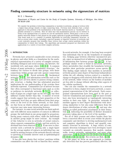
M. E. J. Newman
Department of Physics and Center for the Study of Complex Systems, University of Michigan, Ann Arbor, MI 48109–1040
We consider the problem of detecting communities or modules in networks, groups of vertices with a higher-than-average density of edges connecting them. Previous work indicates that a robust approach to this problem is the maximization of the benefit function known as “modularity” over possible divisions of a network. Here we show that this maximization process can be written in terms of the eigenspectrum of a matrix we call the modularity matrix, which plays a role in community detection similar to that played by the graph Laplacian in graph partitioning calculations. This result leads us to a number of possible algorithms for detecting community structure, as well as several other results, including a spectral measure of bipartite structure in neteasure that identifies those vertices that occupy central positions within the communities to which they belong. The algorithms and measures proposed are illustrated with applications to a variety of real-world complex networks.
Attack vulnerability of complex networks

Attack vulnerability of complex networksPetter Holme*and Beom Jun Kim†Department of Theoretical Physics,Umea˚University,90187Umea˚,SwedenChang No Yoon and Seung Kee HanDepartment of Physics,Chungbuk National University,Cheongju,Chungbuk361-763,Korea͑Received19December2001;published7May2002͒We study the response of complex networks subject to attacks on vertices and edges.Several existing complex network models as well as real-world networks of scientific collaborations and Internet traffic are numerically investigated,and the network performance is quantitatively measured by the average inverse geodesic length and the size of the largest connected subgraph.For each case of attacks on vertices and edges, four different attacking strategies are used:removals by the descending order of the degree and the between-ness centrality,calculated for either the initial network or the current network during the removal procedure.It is found that the removals by the recalculated degrees and betweenness centralities are often more harmful than the attack strategies based on the initial network,suggesting that the network structure changes as important vertices or edges are removed.Furthermore,the correlation between the betweenness centrality and the degree in complex networks is studied.DOI:10.1103/PhysRevE.65.056109PACS number͑s͒:89.75.Fb,89.75.Hc,89.65.ϪsI.INTRODUCTIONExamples of complex networks are abundant in many dis-ciplines of science and have recently received much attention ͓1,2͔.Many works have tried to regenerate geometrical sta-tistics of real-world networks by generative algorithms thatmimic behaviors found in real-world networks.The studiesalong this line have been able to model,e.g.,the emergenceof scale-free degree distributions͓3͔and the high clusteringof social networks͓4,5͔.Another group of complex networkstudies aims to investigate certain dynamical problems onnetwork topologies͓5,6͔.A third group of works studies howthe geometric characteristics and performances of the net-works are affected by the restrictions imposed on networks.The approach taken by the present paper belongs to the thirdcategory as we study the robustness of the network subject tovarious attack strategies.Originated from studies of computer networks,‘‘attackvulnerability’’͓3͔denotes the decrease of network perfor-mance due to a selected removal of vertices or edges.In thepresent study we measure the attack vulnerability of variouscomplex network models and real-world networks.We com-pare different ways of attacking the network and use variousways of measuring the resulting damage.In general,thisgives a measure of the decrease of network functionality un-der a sinister attack.The meaningful purpose for attack vul-nerability studies is for the sake of protection:If one wants toprotect the network by guarding or by a temporary isolationof some vertices͑edges͒,the most important vertices͑edges͒,breaking of which would make the whole network malfunc-tion,should be identified.Furthermore,one can learn how to build attack-robust networks,and also how to increase the robustness of vital biological networks.Also in a large net-work of a criminal organization,the whole network can be made to collapse by arresting key persons,which can be identified by a similar study.However,the applicability to social networks may not be very high—acquaintance ties are to some extent subjective and time dependent͓7͔,and when a social network structure is under attack,the dynamics would probably speed up as the organization tries to protect itself.A topic closely related to attack vulnerability is that of the percolation in complex networks͓8͔,where all vertices͑or edges͒have the equal probability of being disabled.In the network of computers,this situation corresponds to a random breakdown of computers,while in the problem of a disease spread through a network of people,it corresponds to the fact that a randomly chosen set of people are susceptible.One of the key quantities in percolation studies,the size of the larg-est connected subgraph,is also used in the present paper as one of the measures of network performance.This paper is organized as follows:In Sec.II we provide the definitions of terms and measured quantities.In Sec.III various attack strategies are explained.In Sec.IV two real-world networks and several complex network models used in the present paper are briefly described.Sections V,VI,and VII are devoted to the main results,on the relation between degrees and betweenness centralities,on the vulnerability under vertex attack,and on the vulnerability under edge at-tack.Finally,we summarize our results in Sec.VIII.II.DEFINITIONS OF QUANTITIESIn general,the complex networks—networks of both ran-domness and structure—studied in this article can be repre-sented by an undirected and unweighted graph Gϭ(V,E), where V is the set of vertices͑or nodes͒and E is the set of edges͑or links͒.Each edge connects exactly one pair of ver-tices,and a vertex pair can be connected by maximally one edge,i.e.,multiconnection is not allowed.Let,furthermore,*Electronic address:holme@tp.umu.se†Electronic address:kim@tp.umu.se Present address:Departmentof Molecular Science and Technology,Ajou University,Suwon442-749,Korea.PHYSICAL REVIEW E,VOLUME65,056109N denote the number of vertices Nϭ͉V͉and L the number of edges Lϭ͉E͉.For a social network͓9͔,V is a set of persons ͑or‘‘actors’’in the sociology parlance͒and E is the set ofacquaintance ties that links the persons together.In computer networks V represent the routers or computers and E the channels for computer communication.There are several ways of measuring the functionality of networks.One key quantity is the average geodesic length l, which is sometimes termed‘‘the characteristic path length,’’defined bylϵ͗d͑v,w͒͘ϵ1N͑NϪ1͚͒vV͚w vVd͑v,w͒,where d(v,w)is the length of the geodesic between v and w (v,wV),i.e.,the number of edges in the shortest path con-necting the two,and the factor N(NϪ1)is the number of pairs of vertices.If l is large,the dynamics͑of epidemics, informationflow,etc.͒is slow in the network.Social net-works are known to have a very short average geodesic length,lϰln N,with the‘‘six degrees of separation,’’lϷ6, of the earth’s population as a celebrated example͓10͔.The logarithmic increase of l is also characteristic of computer networks,and lϷ17has been estimated for the entire world-wide web͓3͔.As the number of removed vertices or edges is increased,the network will eventually break into disconnected subgraphs.The average geodesic length,by definition,becomes infinite for such a disconnected graph, and one can instead study the average inverse geodesic length,lϪ1ϵͳ1d͑v,w͒ʹϵ1N͑NϪ1͚͒vV͚w vV1d͑v,w͒,͑2.1͒which has afinite value even for a disconnected graph since 1/d(v,w)ϭ0if no path connects v and w.It should be noted that the notation lϪ1does not mean the reciprocal of l.The functionality of the network is then measured by lϪ1:the larger lϪ1is the better the network functions.Since subsequent attacks will disintegrate the network,the size of the largest connected subgraph is also an interesting quantity for measuring the functionality of the networks.In social networks,the largest connected subgraph is known to have a size of the order of the entire network,and accord-ingly is called the‘‘giant component’’͓11͔.Throughout the present paper,we denote the size of the giant component as S,which will be used together with lϪ1to study the attack vulnerability.In addition to the logarithmically increasing average geo-desic length,social networks are found to have a high local transitivity:if͕u,v͖and͕u,w͖are two connected pairs,then v is likely to be connected to w too͑and if it does͕u,v,w͖is called a‘‘triad’’͓͒12͔.The clustering coefficient␥͑intro-duced in Ref.͓5͔͒intends to measure the average degree of the local transitivity in a network:Let͉⌫v͉E denote the num-ber of edges in the neighborhood⌫v of vV,then␥vϵ͉⌫v͉Eͩk v2ͪ͑2.2͒is called the local clustering coefficient of the vertex v.Here the degree k v of v is defined as the number of vertices in⌫v, i.e.,k vϵ͉⌫v͉.The‘‘clustering coefficient’’is then defined as the average of␥v,␥ϵ͗␥v͘ϵ1N͚vV␥v.͑2.3͒An alternative interpretation is that␥v is the fraction of the number of triads divided by the maximal number of triads.In Fig.1,we present an illustration to explain the meaning of the local clustering coefficient:The number of edges within the neighborhood͉⌫v͉Eϭ5and the degree k vϭ6result in ␥vϭ1/3in Fig.1.Both␥v and␥are strictly in the interval ͓0,1͔,with␥ϭ1attained only for a fully connected network, where every vertex is connected to every other vertex with the total number of edges LϭN(NϪ1)/2.Removals of important vertices may affect the network significantly.For example,in Ref.͓3͔only a few removals of vertices with the highest degrees has been shown to be enough to alter the behaviors of scale-free networks and the average geodesic length has been found to increase dramati-cally.In the studies of social networks,centrality is an im-portant concept,which tries to capture the prominence of a person in the embedding social structure.It is natural to ex-pect that removals of vertices with high centrality will worsen the functionality of networks more than the removals by degrees.It should be noted that the vertex with a low degree can have a high centrality͑this will be shown explic-itly in Sec.V͒and thus attacking the network by removing vertices with high centralities may differ from that by de-grees.Among many centrality measures͓14͔we focus on the ‘‘vertex betweenness centrality’’C B(v)͓15͔defined for a vertex vV as follows:C B͑v͒ϭ͚w wЈVwwЈ͑v͒wwЈ,͑2.4͒wherewwЈis the number of geodesics between w and wЈandwwЈ(v)is the number of geodesics between w and wЈFIG.1.An example of how to calculate the local clustering coefficient␥v of the vertex v.The closed black circles indicate the neighborhood⌫v of v,and the thick lines are the edges connecting two vertices within⌫v.Since there arefive such edges(͉⌫v͉E ϭ5)and the degree k vϭ6,we obtain␥vϭ1/3from Eq.͑2.2͒.HOLME,KIM,YOON,AND HAN PHYSICAL REVIEW E65056109that passes v.Similarly,one can define the‘‘edge between-ness centrality’’C B(e)for an edge eE asC B͑e͒ϭ͚w wЈVwwЈ͑e͒wwЈ,͑2.5͒wherewwЈ(e)is the number of geodesics between w and wЈthat includes the edge e.Throughout the present paper, we call C B(v)and C B(e)the vertex betweenness and the edge betweenness for brevity.For calculations of C B(v)and C B(e)we use the O(NL)algorithm presented in Refs.͓16,17͔.III.ATTACK STRATEGIESFor the study of attack vulnerability of the network,the selection procedure of the order in which vertices are re-moved is an open choice.One may of course maximize the destructive effect at anyfixed number of removed vertices ͑or edges͒.However,this requires the knowledge of the whole network structure,and pinpointing the vertex to attack in this way makes a very time-demanding computation.A more tractable choice,used in the original study of computer networks,is to select the vertices in the descending order of degrees in the initial network and then to remove vertices one by one starting from the vertex with the highest degree ͓3͔;this attack strategy uses the initial degree distribution and thus is called‘‘ID removal’’throughout the paper.The vertices with high betweenness also play important roles in connecting vertices in the network͓31͔.The second attack strategy is called‘‘IB removal’’and uses the initial distribu-tion of the betweenness.Both ID removal and IB removal use the information on the initial network.As more vertices are removed,the network structure changes,leading to dif-ferent distributions of the degree and the betweenness than the initial ones.The third attack strategy called‘‘RD re-moval’’uses the recalculated degree distribution at every re-moval step,and the fourth strategy,we call it‘‘RB removal,’’is based on the recalculated betweenness at every step.RD removal has been used in Refs.͓18,19͔.It should be noted that ID and RD removals are local strategies,while the other two based on the betweenness are global ones,which makes the applications of ID and RD O(N)algorithms,while IB and RB are O(NL)even with the best known algorithm ͓16,17͔.The other important difference between the degree-based and the betweenness-based strategies is that the former concentrate on reducing the total number of edges in the network as fast as possible whereas the latter concentrate on destroying as many geodesics as possible.It is not entirely clear a priori which one of these four different attack strat-egies should be more harmful than the others,although one can naively expect that RD and RB are more harmful than ID and IB,respectively.It should also be noted that for the strategies based on the recalculated information,the most harmful sequences for removals of N rm vertices and N rmЈver-tices(N rm N rmЈ)might differ significantly even in the early stage of attacks.One can also attack edges instead of vertices.In the net-work of computers,attacking edges may correspond to the cutting off of communication cables,while the attacks on vertices can be interpreted as breakdowns of servers by ma-licious hackers.͑The opposite is of course also imaginable:a software obstruction of a communication link or a server destroyed physically.͒The vulnerability of networks under edge attacks is also studied by using similar strategies͑we again call them as ID,IB,RD,and RB removals of edges͒. The concept of the edge betweenness was introduced in Sec. II from a straightforward generalization of the vertex be-tweenness.On the other hand,the definition of the‘‘edge degree’’is not so clear.But still it is expected that the im-portance of an edge should be possible to assess by the de-grees of the two vertices it connects.In this work we attempt to define the edge degree k e from the local information of the vertex degrees in several different ways,k eϵk v k w,͑3.1a͒k eϵk vϩk w,͑3.1b͒k eϵmin͑k v,k w͒,͑3.1c͒k eϵmax͑k v,k w͒,͑3.1d͒where the edge e connects two vertices v and w with vertex degrees k v and k w,respectively.As will be discussed in Sec. V,among the above definitions,wefind that Eq.͑3.1a͒gives a more reasonable result͓a higher C B(e)to k e correlation͔than the others,and thus the‘‘edge degree’’defined as k eϵk v k w is used for the attack strategies ID and RD edge removals.From the definitions,we expect that a vertex with higher degree usually should have higher betweenness in most real-world networks.However,the correlation between the edge degree and edge betweenness is less obvious.This is ex-pected to show a larger difference between degree-based and betweenness-based attack strategies for edge attacks than for vertex attack.The four different edge attack strategies ap-plied to a network generated by Watts and Strogatz’s small-world network model͑see Sec.IV D͒is shown in Fig.2. Quite soon the original network structure is lost and procedure-specific structures emerge.For example,the RB edge removal concentrates on edges of high betweenness, and thus edges that carry more geodesics arefirst lost.Con-sequently,it is not a surprise that the resulting network struc-ture by RB consists of highly connected clusters and vertices with no neighbors.The RD procedure,on the other hand, removes edges connecting vertices with high vertex degrees, and,therefore,it is natural that the original network is split into many subgraphs of vertices with low͑but not zero͒de-grees.In Secs.VI and VII,we investigate various networks sub-ject to the above-mentioned four different attack strategies, ID,IB,RD,and RB,applied for vertex removals and edge removals.To detect the damages caused by those attacks,we measure the average inverse geodesic length lϪ1in Eq.͑2.1͒as well as the size S of the giant component.As the vertex attack proceeds,both the remaining number of verti-ces and the average inverse geodesic length decrease,which,ATTACK VULNERABILITY OF COMPLEX NETWORKS PHYSICAL REVIEW E65056109from the definition of l Ϫ1,suggests that l Ϫ1can be both increasing and decreasing,depending on how much damage is made by the removals.However,the edge removals do not change the number of vertices in the network and thus l Ϫ1should be a decreasing function of the number of removed edges.Similarly,S is expected to show different behaviors for vertex and edge removals.For vertex removals,S versus the number of removed vertices should have a slope of unity in the initial attack stages since the removed vertex probably belonged to the giant component.On the other hand,the initial edge attacks should not change the size of the giant component,and thus S versus the number of removed edges should start as a horizontal line.We conclude the section with some technical details:In any case where two or more vertices ͑edges ͒could equally be chosen by some strategy,the selection is done randomly.For the RB strategy,if the betweenness is zero for all verti-ces,i.e.,the vertices are either isolated or linked to exactly one neighbor,the vertices with k v ϭ1are attacked before the meaningless attack of vertices with k v ϭ0.IV .NETWORKSTo study the emergence of different geometrical proper-ties of complex networks such as social networks,power grids,metabolic networks,computer networks,and so on,different generative algorithms have been proposed ͓1͔.Among various existing models for generating networks similar to real ones,two generic models,the Watts-Strogatz ͑WS ͒model of the small-world networks ͓5͔and theBaraba´si-Albert ͑BA ͒model of the scale-free network ͓3,20͔,have been widely studied.Both models commonly show the behavior that two arbitrarily chosen vertices are connected by a remarkably short path.More specifically,the average geodesic length has been found to scale logarithmically with the network size.On the one hand,the WS model does notexhibit the power-law distribution of degree,which many real networks show and the BA model successfully produces.On the other hand,the WS model has high clustering,e.g.,social networks,whereas the BA model has a clustering co-efficient that scales toward zero as N →ϱ.There have been attempts to revise and extend these representative models in order to produce a network model that can show a small average geodesic length,a scale-free degree distribution,and high clustering,all at the same time ͓4,22͔.In this work,we study two real networks,a ‘‘social network’’constructed from scientific collaboration data ͑Sec.IV A ͒and a ‘‘com-puter network’’constructed from computer traffic over the Internet ͑Sec.IV B ͒,as well as four model networks,therandom network model by Erdo¨s and Re ´nyi ͑ER ͒,the WS model,the BA model,and the clustered scale-free network ͑CSF ͒model suggested by two of the present authors in Ref.͓4͔͑Secs.IV C–IV F ͒.It should be noted that network mod-els such as those mentioned above model the emergence of structure in networks—structure that can be monitored by certain quantities such as degree distribution,clustering co-efficient,and so on.However,they do ͑probably ͒not sample the ensemble of networks defined by specific values of these quantities uniformly.This is known to be the case for other ways of generating random graphs with structural biases that are easier to give a probability-theoretical analysis ͓23͔.That the sampling is biased makes an inference from the scaling of quantities difficult—if,e.g.,one model gives networks with the same values as another except for,say,a smaller clustering coefficient,it is not certain that a different behav-ior under,say,edge removal is due to the lower clustering.A.Scientific collaboration network from the hep-late-print archiveTo obtain a well-defined social network from real-world data,we follow Ref.͓17͔and construct a network of scien-tific collaborations from the the Los Alamos preprint ar-chives ͓24͔in the following way:If two scientists wrote an article together,they are connected by an edge.Accordingly,the vertices in the network are scientists,and the edges rep-resent the collaboration ties.For the attack vulnerability cal-culations,the whole Los Alamos e-print archive is too big to be computationally tractable,͓32͔instead we chose the hep-lat database,which contains preprints about lattice studies in high-energy physics,among various subcategories only for computational convenience.The network used in analysis has N ϭ2010͑the number of vertices ͒and L ϭ6614͑the number of edges ͒,and the size of the giant component is S ϭ1412and the clustering coefficient is ␥Ϸ0.571.A discus-sion on the usefulness of collaboration networks as real-world social networks can be found in Ref.͓17͔.puter network from Internet trafficTo build the network structure for the computer commu-nications we follow Ref.͓20͔and use data from the National Laboratory for Applied Network Research ͑NLANR ͓͒25͔.Here the network is constructed as follows:Over a period of 24h a number of servers associated to NLANR and physi-cally spread over USA,gather information throughcomputerFIG.2.Various attack strategies for edge removals applied to a realization of the generative algorithm of the Watts-Strogatz model of small-world network ͑see Sec.IV D ͒.From left to right,the evolutions of network structures are shown for the edge attack strat-egies based on ID ͑initial degree ͒,IB ͑initial betweenness ͒,RD ͑recalculated degree ͒,and RB ͑recalculated betweenness ͒,respec-tively.The initial network structure is displayed at the top left cor-ner of each column and the subsequent structures at the next nine steps are exhibited ͑first four steps from top to bottom and then five more steps from top right to bottom right ͒.For an individual sub-graph the thickness of the lines is proportional to the betweenness of the corresponding edge.HOLME,KIM,YOON,AND HAN PHYSICAL REVIEW E 65056109interconnections.For every connection established through a server the whole path,from the originating vertex to the requested destination,is added to the network graph.To be more specific,the servers are using the border gateway pro-tocol ͑BGP ͒to relay connections over Internet’s largest scale ͓26͔.Vertices are computer networks,or ‘‘autonomous sys-tems’’in BGP nomenclature,interconnected by one or many BGP servers.An edge thus represents an established direct connection between two autonomous systems.The data we analyze represent a network with N ϭS ϭ2210,L ϭ4334,and ␥Ϸ0.221.C.Erdo¨s-Re ´nyi model of random networks In the ER model ͓27͔,we start from N vertices without edges.Subsequently,edges connecting two randomly chosen vertices are added until the total number of edges becomes L .It generates random networks with no particular structural bias:The only restriction in the model is that no multiple edges are allowed between two vertices.In this study,we choose the average degree ͗k ͘ϵ2L /N as a control parameter in the ER model.The ER model graphs have a logarithmi-cally increasing l ,a Poisson-type degree distribution,and a clustering coefficient close to zero.D.Watts-Strogatz model of small-world networksIn the WS model ͓5͔one starts by constructing a regular one-dimensional network with only local connections of range r .For example,r ϭ2means that each vertex is con-nected to its two nearest neighbors and two next nearest neighbors ͓see Fig.3͑a ͔͒.Then each edge is visited once,and with the rewiring probability P ,is detached at the opposite vertex and reconnected to a randomly chosen vertex forming a ‘‘shortcut.’’͑See the illustration in Fig.3.͒For P ϭ0the network is a regular local network,with high clustering,but without the small-world behavior:The average geodesic length in this case grows linearly with the network size.In the opposite limit of P ϭ1,where every edge has been re-wired,the generated random graph has vanishing clustering,but shows a logarithmic behavior of the average geodesic length l ϰln N .In an intermediate range of P ͓typically PϳO (1/N )͔,the network generated by the WS model displays both high clustering and small-world behavior—the com-monly found characteristics of real social networks.E.Baraba´si-Albert model of scale-free networks Apart from the average geodesic length and clustering,the degree distribution is a structural bias that has received much attention.Many ͑but not all ͒real networks are known to have a power-law distribution of degrees ͓3,28͔,manifest-ing a scale-free nature of the network.The BA model of a scale-free network ͓3,20͔is defined by the following ingre-dients:͑1͒Initial condition:To start with the network consists of m 0vertices and no edges.͑2͒Growth:One vertex v with m edges is added every time step.͑3͒Preferential attachment:An edge is added to an old vertex with a probability proportional to its degree.More precisely,the probability P u for a new vertex v to be at-tached to u is ͓33͔:P u ϭk u͚w Vk w.͑4.1͒The growth step is iterated N Ϫm 0times to construct a net-work with size N ,for each growth step the preferential at-tachment step is iterated m times.The above described BA model has been shown to generate scale-free networks with the logarithmically increasing average geodesic length with the size N .However,the original BA model results in net-works with low clustering.F.Clustered scale-free network modelIn order to incorporate the high clustering of social net-works one can modify the standard BA model by adding one additional step,͑4͒Triad formation:If an edge between v and u was added in the previous step of preferential attachment,then add an edge from v to a randomly chosen neighbor w of u .This forms a triad,three vertices connected each other.If there is no available vertex to connect within ⌫u —do a pref-erential attachment step instead.For every new vertex,after an additional preferential at-tachment step,the triad formation step is performed with a probability P t ͑and thus a preferential attachment with the probability 1ϪP t ).The average number of triad formation trials per added vertex m t ϵ(m Ϫ1)P t is taken as a control parameter in this CSF network model ͑see Fig.4͒.The scale-free degree distribution of the original BA model is con-served in the CSF model whose properties have been ana-lyzed in detail in Ref.͓4͔.In the limiting case of m t ϭ0,the original BA network is constructed from the CSF model.The CSF model has been shown to exhibit high clustering ͑fur-thermore,the clustering coefficient is tunable by the control parameter m t ),while it still preserves the characteristics found in the BA model such as the logarithmicallyincreasingFIG.3.The Watts-Strogatz ͑WS ͒model of small-world net-works.The starting point is a regular one-dimensional lattice in ͑a ͒with the range r ϭ2of the connections.Every edge is visited once and then with the rewiring probability P is rewired to the other vertex.The WS model can generate ͑a ͒the local regular network when P ϭ0,with high clustering but with a large average geodesic length,and ͑c ͒the fully random network when P ϭ1,with low clustering but with a very short geodesic length.In the intermediate region of P depicted in ͑b ͒,the WS model has both high clustering and the small-world behavior ͑more specifically,the average geo-desic length l ϰln N for the network with the size N ).ATTACK VULNERABILITY OF COMPLEX NETWORKS PHYSICAL REVIEW E 65056109average geodesic length and the scale-free degree distribu-tion.V .CORRELATION BETWEEN DEGREEAND BETWEENNESSFor the six different networks described in Sec.IV ,we seek the relation between the degree and the betweenness for vertices and edges.Both the degree and the betweenness,to some extent,measure how important the vertex ͑edge ͒is.The natural expectation is that the vertex ͑edge ͒with higher degree should also have higher betweenness.The calculation of the betweenness is based on the global information on paths connecting all pairs of vertices,while the degree,by definition,is the quantity that depends on only the local in-formation.This implies that the identification of the relation between the degree and the betweenness can have practical importance since one can approximately estimate the be-tweenness from the degree.We first show in Fig.5scatter plots of the vertex between-ness C B (v )versus the vertex degree k v .As expected,net-works with the scale-free degree distributions,͑a ͒the scien-tific collaboration network,͑b ͒the computer network,͑e ͒the BA network,and ͑f ͒the CSF network,show clear signs of correlation between the degree and the betweenness.As the scale-free network becomes more clustered ͑from the BA model to the CSF model ͒,the correlation between C B (v )and k v becomes weaker,manifested by more scattered plots in ͑f ͒than ͑e ͒.The ER and the WS models,͑c ͒and ͑d ͒,respec-tively,are characterized by the absence of vertices with very high degrees,which makes the correlation between C B (v )and k v rather difficult to observe especially in the region of high degrees.However,notable correlations are evident even for these networks with an exponential cutoff in degree dis-tributions.For the study of the correlation between the edge degree k e and the edge betweenness C B (e ),we try four different definitions of the edge degree in Eq.͑3.1͒with the assump-tion that the edge degree can be defined by only the degrees of vertices it connects.For all networks,except the scientific collaboration network,we find ͑at least some ͒correlation between k e and C B (e ).This correlation is most evident withthe definition in Eq.͑3.1a ͒,k e ϵk v k w ,where k v and k w are degrees of the vertices v and w that the edge e connects.But the definition k e ϵmin(k v ,k w ),Eq.͑3.1c ͒,also displays a high correlation between k e and C B (e ).This suggests that the lower degree of the two vertices an edge connects is more important for a high edge betweenness than the greater de-gree of the two vertices.In other words,this illustrates the quite natural situation that an edge does not necessarily be-come central just because it connects to one central vertex,rather it has to be a bridge between two central vertices.For the scientific collaboration network,it turns out that none of the definitions of edge degree manifest the correla-tion clearly.Figure 6shows the scatter plots for the edge degree and the edge betweenness,corresponding to the net-works in Fig.5.Especially,the similarity between the real network and the model network is evident between the com-puter network and the CSF network ͓compare ͑b ͒and ͑f ͒inFIG.4.The construction of the clustered scale-free ͑CSF ͒net-work in Sec.IV F.͑a ͒In the preferential attachment step for the newly added vertex v ͑denoted as closed black circle ͒,the white vertex u is chosen with the probability proportional to its degree ͑the dashed line represents the new edge ͒.͑b ͒In the triad formation step an additional edge ͑dashed line ͒is added to a randomly se-lected vertex w in the neighborhood ⌫u of the vertex u chosen in the previous preferential attachment step in ͑a ͒.The vertices marked by ϫare not allowed since they are not in ⌫u .Without the triad formation step,the CSF model reduces to the original BA model of scale-freenetworks.FIG.5.Correlation between the vertex betweenness C B (v )and the vertex degree k v for ͑a ͒the scientific collaboration network,͑b ͒the computer network,͑c ͒the ER network with the size N ϭ104and average degree ͗k ͘ϭ6,͑d ͒the WS network with N ϭ104,r ϭ3,and P ϭ0.01,͑e ͒the BA network with N ϭ104,m 0ϭ5,and m ϭ3,and ͑f ͒the CSF network with N ϭ104,m 0ϭ5,m ϭ3,and m t ϭ1.8͑see Sec.IV for details of networks ͒.All are in log-log scales except for ͑c ͒and ͑d ͒.HOLME,KIM,YOON,AND HAN PHYSICAL REVIEW E 65056109。
深度脉冲神经网络及其应用研究

摘要深度神经网络(Deep Neural Networks, DNNs)作为机器学习(Machine Learning, ML)领域内的研究热点,借鉴生物视觉认知系统的分区机制,将数据表征为一系列的矢量进行特征学习,DNNs在计算机视觉领域取得了巨大成就。
脉冲神经网络(Spiking Neural Networks, SNNs)是一种具有生物可塑性(Biological Plasticity)的神经网络,它利用随时间变化的脉冲序列(Spike Train)在神经元之间进行信息传递,能更好地融入时空信息,是“类脑计算”的主要工具。
结合了DNNs和SNNs各自的优势,分析了现有深度脉冲神经网络(Deep Spiking Neural Networks, DSNNs)的模型特点,开展了脉冲编码、基于DSNNs的学习方法的研究,并针对基于DSNNs的机械臂故障诊断方法进行了研究,具体内容如下:首先,介绍了DSNNs的研究背景和意义,综述了DSNNs的国内外研究现状,阐述了论文的研究内容和技术路线。
其次,介绍了深度卷积神经网络(Deep Convolutional Neural Networks, DCNNs)、深度置信神经网络(Deep Belief Networks, DBNs)以及SNNs的发展、模型结构、现阶段DSNNs模型的实现方法及学习算法等相关内容,为后续研究提供理论支撑。
第三,提出了基于DCNNs的机械臂故障分类方法,重点介绍了UCI机械臂传感数据的预处理技术,分析了DCNNs处理一维时序信号的能力。
将采集到的机械臂力及力矩传感数据在时间和数据两个维度进行结合,并采用1D和2D卷积方法在CPU(Intel Core i5-7200U)和GPU(GFX NVIDIA GeForce GTX1060 3G)进行实验验证。
实验结果表明:对于机械臂一维时序信号数据的处理方式能够很好的拟合DCNNs模型,分类准确率优于传统的分类方法。
外文翻译--神经网络概述

外文原文与译文外文原文Neural Network Introduction1.ObjectivesAs you read these words you are using a complex biological neural network. You have a highly interconnected set of some 1011neurons to facilitate your reading, breathing, motion and thinking. Each of your biological neurons,a rich assembly of tissue and chemistry, has the complexity, if not the speed, of a microprocessor. Some of your neural structure was with you at birth. Other parts have been established by experience.Scientists have only just begun to understand how biological neural networks operate. It is generally understood that all biological neural functions, including memory, are stored in the neurons and in the connections between them. Learning is viewed as the establishment of new connections between neurons or the modification of existing connections.This leads to the following question: Although we have only a rudimentary understanding of biological neural networks, is it possible to construct a small set of simple artificial “neurons” and perhaps train them to serve a useful function? The answer is “yes.”This book, then, is about artificial neural networks.The neurons that we consider here are not biological. They are extremely simple abstractions of biological neurons, realized as elements in a program or perhaps as circuits made of silicon. Networks of these artificial neurons do not have a fraction of the power of the human brain, but they can be trained to perform useful functions. This book is about such neurons, the networks that contain them and their training.2.HistoryThe history of artificial neural networks is filled with colorful, creative individuals from many different fields, many of whom struggled for decades todevelop concepts that we now take for granted. This history has been documented by various authors. One particularly interesting book is Neurocomputing: Foundations of Research by John Anderson and Edward Rosenfeld. They have collected and edited a set of some 43 papers of special historical interest. Each paper is preceded by an introduction that puts the paper in historical perspective.Histories of some of the main neural network contributors are included at the beginning of various chapters throughout this text and will not be repeated here. However, it seems appropriate to give a brief overview, a sample of the major developments.At least two ingredients are necessary for the advancement of a technology: concept and implementation. First, one must have a concept, a way of thinking about a topic, some view of it that gives clarity not there before. This may involve a simple idea, or it may be more specific and include a mathematical description. To illustrate this point, consider the history of the heart. It was thought to be, at various times, the center of the soul or a source of heat. In the 17th century medical practitioners finally began to view the heart as a pump, and they designed experiments to study its pumping action. These experiments revolutionized our view of the circulatory system. Without the pump concept, an understanding of the heart was out of grasp.Concepts and their accompanying mathematics are not sufficient for a technology to mature unless there is some way to implement the system. For instance, the mathematics necessary for the reconstruction of images from computer-aided topography (CAT) scans was known many years before the availability of high-speed computers and efficient algorithms finally made it practical to implement a useful CAT system.The history of neural networks has progressed through both conceptual innovations and implementation developments. These advancements, however, seem to have occurred in fits and starts rather than by steady evolution.Some of the background work for the field of neural networks occurred in the late 19th and early 20th centuries. This consisted primarily of interdisciplinary work in physics, psychology and neurophysiology by such scientists as Hermann vonHelmholtz, Ernst Much and Ivan Pavlov. This early work emphasized general theories of learning, vision, conditioning, etc.,and did not include specific mathematical models of neuron operation.The modern view of neural networks began in the 1940s with the work of Warren McCulloch and Walter Pitts [McPi43], who showed that networks of artificial neurons could, in principle, compute any arithmetic or logical function. Their work is often acknowledged as the origin of theneural network field.McCulloch and Pitts were followed by Donald Hebb [Hebb49], who proposed that classical conditioning (as discovered by Pavlov) is present because of the properties of individual neurons. He proposed a mechanism for learning in biological neurons.The first practical application of artificial neural networks came in the late 1950s, with the invention of the perception network and associated learning rule by Frank Rosenblatt [Rose58]. Rosenblatt and his colleagues built a perception network and demonstrated its ability to perform pattern recognition. This early success generated a great deal of interest in neural network research. Unfortunately, it was later shown that the basic perception network could solve only a limited class of problems. (See Chapter 4 for more on Rosenblatt and the perception learning rule.)At about the same time, Bernard Widrow and Ted Hoff [WiHo60] introduced a new learning algorithm and used it to train adaptive linear neural networks, which were similar in structure and capability to Rosenblatt’s perception. The Widrow Hoff learning rule is still in use today. (See Chapter 10 for more on Widrow-Hoff learning.) Unfortunately, both Rosenblatt's and Widrow's networks suffered from the same inherent limitations, which were widely publicized in a book by Marvin Minsky and Seymour Papert [MiPa69]. Rosenblatt and Widrow wereaware of these limitations and proposed new networks that would overcome them. However, they were not able to successfully modify their learning algorithms to train the more complex networks.Many people, influenced by Minsky and Papert, believed that further research onneural networks was a dead end. This, combined with the fact that there were no powerful digital computers on which to experiment,caused many researchers to leave the field. For a decade neural network research was largely suspended. Some important work, however, did continue during the 1970s. In 1972 TeuvoKohonen [Koho72] and James Anderson [Ande72] independently and separately developed new neural networks that could act as memories. Stephen Grossberg [Gros76] was also very active during this period in the investigation of self-organizing networks.Interest in neural networks had faltered during the late 1960s because of the lack of new ideas and powerful computers with which to experiment. During the 1980s both of these impediments were overcome, and researchin neural networks increased dramatically. New personal computers and workstations, which rapidly grew in capability, became widely available. In addition, important new concepts were introduced.Two new concepts were most responsible for the rebirth of neural net works. The first was the use of statistical mechanics to explain the operation of a certain class of recurrent network, which could be used as an associative memory. This was described in a seminal paper by physicist John Hopfield [Hopf82].The second key development of the 1980s was the backpropagationalgorithm for training multilayer perceptron networks, which was discovered independently by several different researchers. The most influential publication of the backpropagation algorithm was by David Rumelhart and James McClelland [RuMc86]. This algorithm was the answer to the criticisms Minsky and Papert had made in the 1960s. (See Chapters 11 and 12 for a development of the backpropagation algorithm.) These new developments reinvigorated the field of neural networks. In the last ten years, thousands of papers have been written, and neural networks have found many applications. The field is buzzing with new theoretical and practical work. As noted below, it is not clear where all of this will lead US.The brief historical account given above is not intended to identify all of the major contributors, but is simply to give the reader some feel for how knowledge inthe neural network field has progressed. As one might note, the progress has not always been "slow but sure." There have been periods of dramatic progress and periods when relatively little has been accomplished.Many of the advances in neural networks have had to do with new concepts, such as innovative architectures and training. Just as important has been the availability of powerful new computers on which to test these new concepts.Well, so much for the history of neural networks to this date. The real question is, "What will happen in the next ten to twenty years?" Will neural networks take a permanent place as a mathematical/engineering tool, or will they fade away as have so many promising technologies? At present, the answer seems to be that neural networks will not only have their day but will have a permanent place, not as a solution to every problem, but as a tool to be used in appropriate situations. In addition, remember that we still know very little about how the brain works. The most important advances in neural networks almost certainly lie in the future.Although it is difficult to predict the future success of neural networks, the large number and wide variety of applications of this new technology are very encouraging. The next section describes some of these applications.3.ApplicationsA recent newspaper article described the use of neural networks in literature research by Aston University. It stated that "the network can be taught to recognize individual writing styles, and the researchers used it to compare works attributed to Shakespeare and his contemporaries." A popular science television program recently documented the use of neural networks by an Italian research institute to test the purity of olive oil. These examples are indicative of the broad range of applications that can be found for neural networks. The applications are expanding because neural networks are good at solving problems, not just in engineering, science and mathematics, but m medicine, business, finance and literature as well. Their application to a wide variety of problems in many fields makes them very attractive. Also, faster computers and faster algorithms have made it possible to use neuralnetworks to solve complex industrial problems that formerly required too much computation.The following note and Table of Neural Network Applications are reproduced here from the Neural Network Toolbox for MATLAB with the permission of the Math Works, Inc.The 1988 DARPA Neural Network Study [DARP88] lists various neural network applications, beginning with the adaptive channel equalizer in about 1984. This device, which is an outstanding commercial success, is a single-neuron network used in long distance telephone systems to stabilize voice signals. The DARPA report goes on to list other commercial applications, including a small word recognizer, a process monitor, a sonar classifier and a risk analysis system.Neural networks have been applied in many fields since the DARPA report was written. A list of some applications mentioned in the literature follows.AerospaceHigh performance aircraft autopilots, flight path simulations, aircraft control systems, autopilot enhancements, aircraft component simulations, aircraft component fault detectorsAutomotiveAutomobile automatic guidance systems, warranty activity analyzersBankingCheck and other document readers, credit application evaluatorsDefenseWeapon steering, target tracking, object discrimination, facial recognition, new kinds of sensors, sonar, radar and image signal processing including data compression, feature extraction and noise suppression, signal/image identification ElectronicsCode sequence prediction, integrated circuit chip layout, process control, chip failure analysis, machine vision, voice synthesis, nonlinear modeling EntertainmentAnimation, special effects, market forecastingFinancialReal estate appraisal, loan advisor, mortgage screening, corporate bond rating, credit line use analysis, portfolio trading program, corporate financial analysis, currency price predictionInsurancePolicy application evaluation, product optimizationManufacturingManufacturing process control, product design and analysis, process and machine diagnosis, real-time particle identification, visual quality inspection systems, beer testing, welding quality analysis, paper quality prediction, computer chip quality analysis, analysis of grinding operations, chemical product design analysis, machine maintenance analysis, project bidding, planning and management, dynamic modeling of chemical process systemsMedicalBreast cancer cell analysis, EEG and ECG analysis, prosthesis design, optimization of transplant times, hospital expense reduction, hospital quality improvement, emergency room test advisement0il and GasExplorationRoboticsTrajectory control, forklift robot, manipulator controllers, vision systems SpeechSpeech recognition, speech compression, vowel classification, text to speech synthesisSecuritiesMarket analysis, automatic bond rating, stock trading advisory systems TelecommunicationsImage and data compression, automated information services,real-time translation of spoken language, customer payment processing systemsTransportationTruck brake diagnosis systems, vehicle scheduling, routing systems ConclusionThe number of neural network applications, the money that has been invested in neural network software and hardware, and the depth and breadth of interest in these devices have been growing rapidly.4.Biological InspirationThe artificial neural networks discussed in this text are only remotely related to their biological counterparts. In this section we will briefly describe those characteristics of brain function that have inspired the development of artificial neural networks.The brain consists of a large number (approximately 1011) of highly connected elements (approximately 104 connections per element) called neurons. For our purposes these neurons have three principal components: the dendrites, the cell body and the axon. The dendrites are tree-like receptive networks of nerve fibers that carry electrical signals into the cell body. The cell body effectively sums and thresholds these incoming signals. The axon is a single long fiber that carries the signal from the cell body out to other neurons. The point of contact between an axon of one cell and a dendrite of another cell is called a synapse. It is the arrangement of neurons and the strengths of the individual synapses, determined by a complex chemical process, that establishes the function of the neural network. Figure 6.1 is a simplified schematic diagram of two biological neurons.Figure 6.1 Schematic Drawing of Biological NeuronsSome of the neural structure is defined at birth. Other parts are developed through learning, as new connections are made and others waste away. This development is most noticeable in the early stages of life. For example, it has been shown that if a young cat is denied use of one eye during a critical window of time, it will never develop normal vision in that eye.Neural structures continue to change throughout life. These later changes tend to consist mainly of strengthening or weakening of synaptic junctions. For instance, it is believed that new memories are formed by modification of these synaptic strengths. Thus, the process of learning a new friend's face consists of altering various synapses.Artificial neural networks do not approach the complexity of the brain. There are, however, two key similarities between biological and artificial neural networks. First, the building blocks of both networks are simple computational devices (although artificial neurons are much simpler than biological neurons) that are highly interconnected. Second, the connections between neurons determine the function of the network. The primary objective of this book will be to determine the appropriate connections to solve particular problems.It is worth noting that even though biological neurons are very slow whencompared to electrical circuits, the brain is able to perform many tasks much faster than any conventional computer. This is in part because of the massively parallel structure of biological neural networks; all of the neurons are operating at the same time. Artificial neural networks share this parallel structure. Even though most artificial neural networks are currently implemented on conventional digital computers, their parallel structure makes them ideally suited to implementation using VLSI, optical devices and parallel processors.In the following chapter we will introduce our basic artificial neuron and will explain how we can combine such neurons to form networks. This will provide a background for Chapter 3, where we take our first look at neural networks in action.译文神经网络概述1.目的当你现在看这本书的时候,就正在使用一个复杂的生物神经网络。
- 1、下载文档前请自行甄别文档内容的完整性,平台不提供额外的编辑、内容补充、找答案等附加服务。
- 2、"仅部分预览"的文档,不可在线预览部分如存在完整性等问题,可反馈申请退款(可完整预览的文档不适用该条件!)。
- 3、如文档侵犯您的权益,请联系客服反馈,我们会尽快为您处理(人工客服工作时间:9:00-18:30)。
Protein Interaction Network
Proteins in a cell
There are thousands of different active proteins in a cell acting as:
enzymes, catalysors to chemical reactions of the metabolism components of cellular machinery (e.g. ribosomes) regulators of gene expression Certain proteins play specific roles in special cellular compartments. Others move from one compartment to another as “signals”.
Pathway Networks
Signaling & Metabolic Pathway Network
A Pathway can be defined as a modular unit of interacting molecules to fulfill a cellular function.
Database / Knowledge Source
Homology Modeling
Post-tranlational Modification
Database / Knowledge Source
From the particular to the universal
A.-L- Barabasi & Z. Oltvai, Science, 2002
Why Study Networks?
It is increasingly recognized that complex systems cannot be described in a reductionist view. Understanding the behavior of such systems starts with understanding the topology of the corresponding network. Topological information is fundamental in constructing realistic models for the function of the network.
Protein Interactions
P. Uetz, et al. Nature, 2000; Ito et al., PNAS, 2001; …
Yeast Protein Interaction Network
Nodes: proteins
Links: physical
interactions (binding)
Bioinformatics
The essence of life is information (i.e. from digital code to emerging properties of biosystems.)
Bioinformatics is the study of information content of life
Power Law Network
PREFERENTIAL ATTACHMENT on Growth: the probability that a new vertex will be connected to vertex i depends on the connectivity of that vertex:
Biological Networks’ Properties Databases Discussion STM Clustering Model
Introduction
Bioinformatics
Informatics
Its carrier is a set of digital codes and a language. In its manifestation in the space-time continuum, it has utility (e.g. to decrease entropy of an open system).
Biological Network Model
Network
A linked list of interconnected nodes.
Node
Protein, peptide, or non-protein biomolecules.
Edges
Biological relationships, etc., interactions, regulations, reactions,
Regulatory Network
Expression Network
A network representation of genomic data. Inferred from genomic data, i.e. microarray.
BIOLOGICAL NETWORK PROPERTY
A Pathway Example
A Pathway Example
A Pathway Example
Regulatory Network
a collection of DNA segments (genes) in a cell which interact with each other and with other substances in the cell, thereby governing the rates at which genes in the network are transcribed into mRNA.
Proteomics
Genomics Proteomics
Structural Proteomics
Structure Determination
Functional Proteomics
Protein-Protein Interaction & Networking Protein Expression
Interaction Network Pathway Network Regulatory Network Expression Network
Biological Networks Properties
Power law degree distribution: Rich get richer Small World: A small average path length Mean shortest node-to-node path Robustness: Resilient and have strong resistance to failure on random attacks and vulnerable to targeted attacks Hierarchical Modularity: A large clustering coefficient How many of a node’s neighbors are connected to each other
Genome Size
Proteom Sizeቤተ መጻሕፍቲ ባይዱ(PDB)
BIOLOGICAL NETWORK
Networks are found in biological systems of varying scales:
1. Evolutionary tree of life 2. Ecological networks 3. Expression networks 4. Regulatory networks - genetic control networks of organisms 5. The protein interaction network in cells 6. The metabolic network in cells … more biological networks
Protein Interactions
Proteins perform a function as a complex rather as a single protein. Knowing whether two proteins interact can help us discover unknown proteins’ functions: If the function of one protein is known, the function of its binding partners are likely to be related- “guilt by association”. Thus, having a good method for detecting interactions can allow us to use a small number of proteins with known function to characterize new proteins.
Signaling Pathway Networks
Metabolic Pathway Networks
In biology a signal or biopotential is an electric quantity (voltage or current or field strength), caused by chemical reactions of charged ions. refer to any process by which a cell converts one kind of signal or stimulus into another. Another use of the term lies in describing the transfer of information between and within cells, as in signal transduction. a series of chemical reactions occurring within a cell, catalyzed by enzymes, resulting in either the formation of a metabolic product to be used or stored by the cell, or the initiation of another metabolic pathway