2 Counting Convex Polyominoes According to Their Area
泊松融合原理和python代码

泊松融合原理和python代码【原创版】目录1.泊松融合原理概述2.Python 代码实现泊松融合原理3.泊松融合原理的应用正文1.泊松融合原理概述泊松融合原理是一种概率论中的经典理论,由法国数学家泊松提出。
泊松融合原理描述了一个事件在特定时间间隔内发生的概率与另一个事件在相同时间间隔内发生的次数之间的关系。
具体而言,泊松融合原理表明,一个事件在时间间隔Δt 内发生的次数服从泊松分布,即P(X=k)=e^(-λΔt) * (λΔt)^k / k!,其中λ是事件的平均发生率,X 是事件在时间间隔Δt 内发生的次数,k 是事件发生的次数。
2.Python 代码实现泊松融合原理为了验证泊松融合原理,我们可以使用 Python 编写代码模拟事件的发生过程。
以下是一个简单的 Python 代码示例:```pythonimport randomimport mathdef poisson_fusion(lambda_value, dt, num_trials):"""泊松融合原理模拟:param lambda_value: 事件的平均发生率:param dt: 时间间隔:param num_trials: 模拟次数:return: 事件在时间间隔内发生的次数"""count = 0for _ in range(num_trials):# 随机生成一个 0 到 dt 之间的时间间隔t = random.uniform(0, dt)# 计算在时间间隔内事件发生的次数k = int(lambda_value * t)# 计算泊松分布的概率poisson_prob = math.exp(-lambda_value * t) * (lambda_value * t) ** k / k# 根据泊松分布概率随机生成事件发生的次数count += random.choice([0, 1, 2, 3, 4],p=poisson_prob)return count# 示例lambda_value = 1 # 事件的平均发生率为 1dt = 1 # 时间间隔为 1um_trials = 1000 # 模拟次数为 1000# 模拟事件在时间间隔内发生的次数counts = [poisson_fusion(lambda_value, dt, num_trials) for _in range(num_trials)]# 计算平均值和方差mean = sum(counts) / num_trialsvariance = sum((count - mean) ** 2 for count in counts) / num_trialsprint("平均值:", mean)print("方差:", variance)```3.泊松融合原理的应用泊松融合原理在实际应用中有很多场景,例如统计学、保险、生物学等领域。
模式识别第二版答案完整版
模式识别(第二版)习题解答
目录
1 绪论
2
2 贝叶斯决策理论
2
j=1,...,c
类条件概率相联系的形式,即 如果 p(x|wi)P (wi) = max p(x|wj)P (wj),则x ∈ wi。
j=1,...,c
• 2.6 对两类问题,证明最小风险贝叶斯决策规则可表示为,若
p(x|w1) > (λ12 − λ22)P (w2) , p(x|w2) (λ21 − λ11)P (w1)
max P (wj|x),则x ∈ wj∗。另外一种形式为j∗ = max p(x|wj)P (wj),则x ∈ wj∗。
j=1,...,c
j=1,...,c
考虑两类问题的分类决策面为:P (w1|x) = P (w2|x),与p(x|w1)P (w1) = p(x|w2)P (w2)
是相同的。
• 2.9 写出两类和多类情况下最小风险贝叶斯决策判别函数和决策面方程。
λ11P (w1|x) + λ12P (w2|x) < λ21P (w1|x) + λ22P (w2|x) (λ21 − λ11)P (w1|x) > (λ12 − λ22)P (w2|x)
(λ21 − λ11)P (w1)p(x|w1) > (λ12 − λ22)P (w2)p(x|w2) p(x|w1) > (λ12 − λ22)P (w2) p(x|w2) (λ21 − λ11)P (w1)
协方差核函数

协方差核函数协方差核函数(Covariance Kernel Function)是机器学习领域中常用的一种核函数。
核函数是一种能够将输入空间中的向量映射到特征空间中的函数,可以用于解决非线性分类和回归问题。
在支持向量机(Support Vector Machine)中,核函数的选择对于模型的性能和泛化能力起到至关重要的作用。
协方差核函数的提出主要是基于协方差矩阵的性质。
协方差矩阵是一个对称的正定矩阵,描述了数据中各维度之间的相关性。
协方差核函数通过计算两个样本之间的协方差矩阵,来度量它们的相似性。
在机器学习中,常常需要对输入数据进行特征映射,将原始的低维数据映射到高维特征空间中,以便更好地进行分类或回归。
协方差核函数可以在不显示地进行特征映射的情况下,直接在原始空间中计算两个样本之间的相似性。
具体来说,协方差核函数可以通过计算两个样本之间的协方差矩阵的行列式来度量它们的相似性。
协方差矩阵的行列式表示了数据的离散程度,行列式越大,表示数据在各个维度上的差异越大,样本之间的相似性越低;行列式越小,表示数据在各个维度上的差异越小,样本之间的相似性越高。
通过使用协方差核函数,可以将原始数据的离散程度转化为样本相似性的度量。
协方差核函数的优点是能够在不显示地进行特征映射的情况下,直接度量样本之间的相似性。
这样可以大大减少计算量,并且避免了特征映射过程中可能引入的噪声和误差。
此外,协方差核函数还具有良好的数学性质,能够满足核函数的一些要求,如正定性和对称性。
然而,协方差核函数也存在一些局限性。
首先,协方差核函数的计算复杂度较高,特别是在高维数据集上。
其次,协方差核函数对数据的分布有一定的假设,如果数据的分布不满足这些假设,可能会导致模型的性能下降。
此外,由于协方差核函数直接度量样本之间的相似性,可能会忽略样本之间的局部结构信息。
总的来说,协方差核函数是一种常用且有效的核函数,能够在不显示地进行特征映射的情况下,直接度量样本之间的相似性。
separable convolution公式
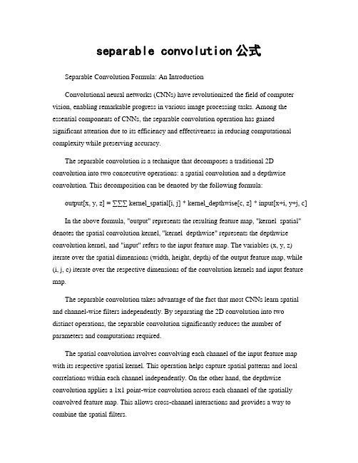
separable convolution公式Separable Convolution Formula: An IntroductionConvolutional neural networks (CNNs) have revolutionized the field of computer vision, enabling remarkable progress in various image processing tasks. Among the essential components of CNNs, the separable convolution operation has gained significant attention due to its efficiency and effectiveness in reducing computational complexity while preserving accuracy.The separable convolution is a technique that decomposes a traditional 2D convolution into two consecutive operations: a spatial convolution and a depthwise convolution. This decomposition can be denoted by the following formula:output[x, y, z] = ∑∑∑ kernel_spatial[i, j] * kernel_depthwise[c, z] * input[x+i, y+j, c]In the above formula, "output" represents the resulting feature map, "kernel_spatial" denotes the spatial convolution kernel, "kernel_depthwise" represents the depthwise convolution kernel, and "input" refers to the input feature map. The variables (x, y, z) iterate over the spatial dimensions (width, height, depth) of the output feature map, while (i, j, c) iterate over the respective dimensions of the convolution kernels and input feature map.The separable convolution takes advantage of the fact that most CNNs learn spatial and channel-wise filters independently. By separating the 2D convolution into two distinct operations, the separable convolution significantly reduces the number of parameters and computations required.The spatial convolution involves convolving each channel of the input feature map with its respective spatial kernel. This operation helps capture spatial patterns and local correlations within each channel independently. On the other hand, the depthwise convolution applies a 1x1 point-wise convolution across each channel of the spatially convolved feature map. This allows cross-channel interactions and provides a way to combine the spatial filters.Compared to the standard 2D convolution, separable convolution offers several advantages. First, it greatly reduces computational complexity, resulting in faster inference and training times. Second, it alleviates overfitting by reducing the capacity of the model, preventing excessive memorization. Lastly, the separable convolution can achieve similar or even better performance compared to the standard convolution in many scenarios.In conclusion, the separable convolution formula provides a powerful technique that enhances the efficiency and effectiveness of convolutional neural networks. By decomposing the traditional 2D convolution into spatial and depthwise convolutions, separable convolution reduces computational complexity while maintaining accuracy. This technique has become a fundamental building block in modern CNN architectures, enabling remarkable advancements in image processing tasks.。
人工智能核函数例题

人工智能核函数例题
人工智能中的核函数是一种用于支持向量机(SVM)和其他机器
学习算法的工具。
核函数可以把输入数据映射到高维空间,从而使
得原本在低维空间中线性不可分的数据在高维空间中变得线性可分。
这样一来,我们就可以使用线性分类器来处理这些数据。
举个例子,假设我们有一组二维数据点,它们在二维平面上是
线性不可分的。
但是,如果我们使用一个二次多项式核函数,它可
以将这些二维数据点映射到三维空间中,使得它们在三维空间中变
得线性可分。
这样一来,我们就可以使用一个平面来分隔这些数据点,实现了在原始的二维空间中无法实现的分类。
另一个常见的核函数是高斯核函数(也称为径向基函数)。
这
个核函数可以将数据映射到无限维的特征空间中,从而可以处理非
线性可分的数据。
除了上述的例子之外,核函数还可以是多项式核函数、字符串
核函数等等。
它们在不同的机器学习问题中发挥着重要的作用,能
够帮助算法更好地处理复杂的数据集。
总之,核函数在人工智能中扮演着至关重要的角色,它们可以
帮助我们处理线性不可分的数据,拓展了机器学习算法的应用范围。
通过合理选择和使用核函数,我们可以更好地解决各种复杂的实际
问题。
(repblock)的多分枝卷积结构
在深度学习领域中,(repblock)的多分枝卷积结构是一种非常有前景的模型架构。
这种结构将特征提取和信息整合的过程分解成多个分支,使得模型可以更好地适应不同尺度和不同方向的特征。
在本文中,我将对这一主题进行全面评估,并撰写一篇有价值的文章,以便你更加深入地了解这一模型结构。
让我们来谈谈(repblock)的多分枝卷积结构的基本概念。
这种结构是由多个分支组成的,每个分支可以专门负责提取不同尺度或方向的特征。
通过这种多分支的方式,模型可以更全面地捕捉输入数据的特征,从而提高模型对复杂问题的建模能力。
这种结构的灵活性和高效性使其在图像、语音、自然语言处理等领域都有广泛的应用前景。
接下来,让我们深入探讨(repblock)的多分枝卷积结构在实际应用中的优势和局限性。
这种结构可以有效地解决特征提取的多尺度和多方向性问题,提高模型对输入数据的表征能力,使得模型更加鲁棒和全面。
另多分枝结构也存在着训练复杂度较高、参数调优困难等问题,需要深入研究和实践中不断优化。
在总结回顾方面,(repblock)的多分枝卷积结构的优势在于能够更全面地提取输入数据的特征,从而提高模型的建模能力;而其局限性则在于训练复杂度高、参数调优困难等问题。
在个人观点和理解方面,我认为这种结构在未来的深度学习研究和应用中将会有更广泛的发展,但需要结合具体场景和问题进行灵活应用和优化。
(repblock)的多分枝卷积结构是一种非常有前景的模型结构,具有很高的研究和应用价值。
通过本文的深入探讨,相信你已经对这一主题有了更加全面、深刻和灵活的理解。
希望本文能够对你有所帮助,期待与你共同探讨更多深度学习领域的热点主题。
在深度学习领域中,(repblock)的多分枝卷积结构在近年来备受关注,被认为是一种非常有前景的模型架构。
这种结构通过将特征提取和信息整合的过程分解成多个分支,使得模型可以更好地适应不同尺度和不同方向的特征,从而提高模型的表征能力和建模能力。
polynomialfeatures用法
一、PolynomialFeatures简介PolynomialFeatures是scikit-learn中的一个函数,用于生成一个新的特征矩阵,其中包含所有的组合特征,用于多项式回归或其他高阶模型。
在机器学习中,有时候通过添加高次项自变量的幂函数来拟合一些非线性模型。
这时候可以使用PolynomialFeatures函数来自动生成这些高次项的特征变量。
二、PolynomialFeatures的基本用法在scikit-learn中使用PolynomialFeatures函数非常简单,只需按照以下步骤即可:1.导入PolynomialFeatures函数在代码中首先需要导入PolynomialFeatures函数,一般位于`sklearn.preprocessing`模块中。
2.创建PolynomialFeatures对象接下来需要创建一个PolynomialFeatures对象,可以通过指定`degree`参数来设置生成的多项式阶数,还可以设置`include_bias`参数来决定是否包含截距项。
3.拟合与转换将原始的特征矩阵传入PolynomialFeatures对象的`fit_transform`方法,即可得到包含多项式特征的新特征矩阵。
4.应用到模型中可以将生成的多项式特征矩阵应用到机器学习模型中进行训练和预测。
三、PolynomialFeatures的参数说明PolynomialFeatures函数主要包含以下几个常用参数:1. degree:整数型参数,表示多项式的阶数。
2. interaction_only:布尔型参数,默认为False,表示是否只生成特征的交互项,若为True则只生成特征之间的乘积项。
3. include_bias:布尔型参数,默认为True,表示是否在生成的多项式特征中包含截距项。
四、示例代码以下是一个简单的示例代码,演示了如何使用PolynomialFeatures生成多项式特征。
常见的核函数

常见的核函数核函数是机器学习中一种常用的方法,它主要用于将高维空间中的数据映射到低维空间中,从而提升算法的性能。
核函数在SVM、PCA、KPCA等机器学习算法中广泛应用。
下面我们将介绍常见的核函数。
1. 线性核函数线性核函数是最简单的核函数之一,它是一种将数据点映射到低维空间的方式,其表达式如下:K(x_i, x_j) = (x_i * x_j)其中x_i, x_j是样本数据集中的两个数据,返回一个标量值。
线性核函数的优点在于需要的计算量较小,适用于大型数据集,但它的缺点是它只能处理线性分离的数据。
2. 多项式核函数其中x_i, x_j是样本数据集中的两个数据,c是一个常数,d是多项式的度数。
多项式核函数适用于非线性分离的数据。
3. 径向基函数(RBF)核函数其中x_i, x_j是样本数据集中的两个数据,gamma是一个正常数,||x_i - x_j||^2表示两个数据点之间的欧几里得距离的平方。
4. Sigmoid核函数其中x_i, x_j是样本数据集中的两个数据,alpha和beta是Sigmoid函数参数。
Sigmoid核函数适用于二分类问题。
上述四种核函数都是常见的核函数,它们各自有不同的优劣势,在不同的机器学习算法中应该选择适当的核函数来处理不同的数据。
除了上述四种常见的核函数,还有其他的一些核函数也具有重要的应用价值。
5. Laplacian核函数Laplacian核函数计算方式类似于径向基函数,但是它将样本数据点间的距离转化成样本数据点间的相似度,其表达式如下:K(x_i, x_j) = exp(-gamma * ||x_i - x_j||)其中gamma和径向基函数中的参数相同。
Laplacian核函数在图像识别和自然语言处理等领域有着广泛的应用。
6. ANOVA核函数ANOVA核函数通常用于数据分析和统计学中,它对混合多种类型数据的模型有较好的表现,其表达式如下:其中h_i和h_j是从样本数据点中提取出来的特征,gamma是一个常数。
text2vec embedding 原理
text2vec embedding 原理
text2vec是一种用于文本嵌入(text embedding)的方法。
它使用了词袋模型(bag-of-words model)和分布式假设(distributed hypothesis),通过将文本表示为向量形式来捕捉单词之间的语义关联。
text2vec的主要原理如下:1. 词袋模型:text2vec首先将文本分割成单词,并将每个单词表示为独立的特征。
这种表示方式忽略了单词在上下文中的顺序,只关注每个单词出现的频率。
2. 局部上下文窗口:为了捕捉到单词之间的语义关联,text2vec引入了局部上下文窗口。
对于每个单词,它考虑其前后固定数量的单词作为上下文,并通过计算上下文中不同单词的共现次数来建立单词之间的共现矩阵。
3. 正负样本采样:为了构建训练数据,text2vec使用了负采样(negative sampling)的方法。
对于每个正样本组合(两个共现的单词),它从语料库中随机选择一些负样本组合(两个未共现的单词)。
这样可以在训练过程中更好地控制正负样本的比例,提高模型的效果。
4. 嵌入学习:text2vec使用了skip-gram模型来学习单词的嵌入表示。
skip-gram模型的目标是通过最大化给定上下文单词的条件概率来学习单词的向量表示。
具体来说,对于每个上下文单词,skip-gram模型尝试预测与之共现的单词。
模型的参数通过最大化条件概率的对数来进行训练。
通过这些步骤,text2vec可以将文本中的单词表示为高维向量,其中每个维度对应于一个语义特征。
这些向量可以用于各种文本处理任务,如文本分类、聚类和信息检索等。
纹理物体缺陷的视觉检测算法研究--优秀毕业论文
摘 要
在竞争激烈的工业自动化生产过程中,机器视觉对产品质量的把关起着举足 轻重的作用,机器视觉在缺陷检测技术方面的应用也逐渐普遍起来。与常规的检 测技术相比,自动化的视觉检测系统更加经济、快捷、高效与 安全。纹理物体在 工业生产中广泛存在,像用于半导体装配和封装底板和发光二极管,现代 化电子 系统中的印制电路板,以及纺织行业中的布匹和织物等都可认为是含有纹理特征 的物体。本论文主要致力于纹理物体的缺陷检测技术研究,为纹理物体的自动化 检测提供高效而可靠的检测算法。 纹理是描述图像内容的重要特征,纹理分析也已经被成功的应用与纹理分割 和纹理分类当中。本研究提出了一种基于纹理分析技术和参考比较方式的缺陷检 测算法。这种算法能容忍物体变形引起的图像配准误差,对纹理的影响也具有鲁 棒性。本算法旨在为检测出的缺陷区域提供丰富而重要的物理意义,如缺陷区域 的大小、形状、亮度对比度及空间分布等。同时,在参考图像可行的情况下,本 算法可用于同质纹理物体和非同质纹理物体的检测,对非纹理物体 的检测也可取 得不错的效果。 在整个检测过程中,我们采用了可调控金字塔的纹理分析和重构技术。与传 统的小波纹理分析技术不同,我们在小波域中加入处理物体变形和纹理影响的容 忍度控制算法,来实现容忍物体变形和对纹理影响鲁棒的目的。最后可调控金字 塔的重构保证了缺陷区域物理意义恢复的准确性。实验阶段,我们检测了一系列 具有实际应用价值的图像。实验结果表明 本文提出的纹理物体缺陷检测算法具有 高效性和易于实现性。 关键字: 缺陷检测;纹理;物体变形;可调控金字塔;重构
Keywords: defect detection, texture, object distortion, steerable pyramid, reconstruction
II
convlstm结构与公式详解
convlstm结构与公式详解ConvLSTM是一种特殊的LSTM(长短时记忆)结构,主要用于处理具有空间依赖性的序列数据,如视频帧、气候数据等。
ConvLSTM通过引入卷积运算来改进LSTM,使其能够更好地处理具有空间结构的数据。
ConvLSTM的结构主要包括以下部分:1.输入层:输入数据为三维张量,其中最后一个维度表示时间序列的长度。
2.输入门(Input Gate):用于更新细胞状态。
通过卷积运算和sigmoid激活函数,根据当前输入和上一个时刻的细胞状态计算得到。
3.遗忘门(Forget Gate):用于决定哪些信息需要被遗忘。
通过卷积运算和sigmoid激活函数,根据当前输入和上一个时刻的细胞状态计算得到。
4.输出门(Output Gate):用于决定当前时刻的输出。
通过卷积运算和tanh激活函数,根据当前输入、上一个时刻的细胞状态和输入门计算得到。
5.细胞状态:通过输入门、遗忘门和输出门的计算结果进行更新和调整。
6.输出层:将细胞状态通过tanh激活函数进行转换,得到最终的输出。
ConvLSTM的公式主要包括以下部分:1.输入门:i_t = sigmoid(W_ii * x_t + b_ii + W_hi * h_{t-1} + b_hi)2.遗忘门:f_t = sigmoid(W_if * x_t + b_if + W_hf * h_{t-1} + b_hf)3.输出门:o_t = tanh(W_io * x_t + b_io + W_ho * h_{t-1} + b_ho)4.细胞状态:c_t = f_t * c_{t-1} + i_t * o_t5.输出:h_t = tanh(c_t)其中,W和b分别为权重和偏置项,x为输入数据,h为输出数据,c为细胞状态,i、f、o 分别为输入门、遗忘门和输出门的计算结果。
如何处理卷积神经网络中的类别不平衡问题

如何处理卷积神经网络中的类别不平衡问题卷积神经网络(Convolutional Neural Networks,简称CNN)是一种在计算机视觉领域广泛应用的深度学习模型。
它通过多层卷积和池化操作来提取图像的特征,并通过全连接层进行分类或回归任务。
然而,在实际应用中,我们经常会遇到一个问题,那就是类别不平衡。
类别不平衡是指训练数据中不同类别的样本数量差异过大的情况。
例如,在一个二分类问题中,正样本的数量远远小于负样本的数量。
这种情况下,CNN往往会倾向于将样本分类为数量较多的类别,而忽略了数量较少的类别。
为了解决类别不平衡问题,我们可以采取以下几种方法。
首先,一种常见的方法是重采样。
这种方法通过增加少数类别的样本数量或减少多数类别的样本数量来达到平衡的效果。
常用的重采样方法包括过采样和欠采样。
过采样是指通过复制少数类别的样本来增加其数量,而欠采样则是通过删除多数类别的样本来减少其数量。
这种方法的优点是简单易行,但也存在一些问题,比如过采样容易导致过拟合,而欠采样可能会丢失一些重要的信息。
其次,另一种方法是修改损失函数。
在CNN中,通常使用交叉熵作为损失函数来衡量模型预测结果与真实标签之间的差异。
当类别不平衡时,我们可以修改交叉熵损失函数,引入类别权重来平衡不同类别之间的重要性。
具体来说,可以通过给少数类别赋予较大的权重,使模型更加关注少数类别。
这种方法的优点是简单有效,但需要手动调整类别权重,可能需要一定的经验和领域知识。
另外,一种更加复杂的方法是引入样本生成技术。
这种方法通过生成新的样本来平衡不同类别之间的数量差异。
常用的样本生成技术包括SMOTE(Synthetic Minority Over-sampling Technique)和GAN(Generative Adversarial Networks)。
SMOTE通过在少数类别样本之间插值生成新的样本,从而增加其数量。
而GAN则通过生成器和判别器的对抗训练来生成逼真的少数类别样本。
silhouette函数确定聚类个数原理

silhouette函数确定聚类个数原理
Silhouette函数是一种用于确定聚类个数的方法,它通过计算
每个样本的轮廓系数来评估聚类的效果。
轮廓系数反映了样本与其所属簇的密集程度,值越大表示样本聚类得更好。
聚类个数的确定是一个重要的问题,影响聚类结果的准确性和有效性。
通常,在使用聚类算法进行分析时,我们需要提前确定聚类的个数。
通常情况下,我们希望聚类之间的差异越大越好,即聚类的内部紧密程度较高,不同聚类之间的分隔程度较大。
Silhouette函数根据下面的公式计算每个样本的轮廓系数:
s(i) = (b(i) - a(i))/max(a(i), b(i))
其中,a(i)表示样本i与同簇其他样本的平均距离,b(i)表示样
本i与其他簇最近样本的平均距离。
所以,轮廓系数越接近1,表示样本聚类得越好;轮廓系数越接近-1,表示样本更应该属
于另外的簇;轮廓系数越接近0,表示样本在两个簇之间的边界,或者样本离聚类边界很远。
通过计算每个样本的轮廓系数,我们可以得到一个聚类的平均轮廓系数,用于评价整个聚类的效果。
为了确定合适的聚类个数,我们可以尝试不同的聚类个数,计算平均轮廓系数,选择平均轮廓系数最大的个数作为最佳的聚类个数。
总结起来,轮廓系数根据样本内部的紧密程度和不同聚类之间
的分隔程度来评估聚类的效果,通过计算每个样本的轮廓系数,并选择平均轮廓系数最大的聚类个数,可以确定最佳的聚类个数。
卷积 维特比译码 c语言
卷积维特比译码c语言卷积码和维特比(Viterbi)译码是两种在通信系统中常用的编码和解码技术。
卷积码是一种线性分组码,它通过将输入信息序列与一组预定的约束条件进行卷积运算来生成编码序列。
而维特比译码是一种高效的解码算法,用于从接收到的信号中恢复出原始的编码序列。
下面是一个简单的C语言示例,演示了如何实现卷积编码和维特比译码。
请注意,这只是一个基本的示例,实际的实现可能会更复杂,并且需要更多的错误处理和优化。
c复制代码:#include <stdio.h>#include <stdlib.h>#define N 4#define K 2#define G 2// 卷积编码函数void convolutional_encode(int input[K], int code[N]) {int i, j;for (i = 0; i < N; i++) {code[i] = 0;}for (i = 0; i < K; i++) {code[i] = input[i];}for (i = K; i < N; i++) {code[i] = (code[i - 1] ^ code[i - 2]) & G;}}// 维特比译码函数void viterbi_decode(int received[N], int output[K]) {int branch_metric[N][2];int path_metric[N];int max_metric, new_max_metric;int max_path, new_max_path;int i, j, k;for (i = 0; i < N; i++) {path_metric[i] = abs(received[i] - 0); // 初始化路径度量branch_metric[i][0] = abs(received[i] - 0); // 初始化分支度量branch_metric[i][1] = abs(received[i] - G); // 初始化分支}for (i = 0; i < N; i++) {output[i] = 0; // 初始化输出序列}for (i = 0; i < N; i++) {if (branch_metric[i][0] > branch_metric[i][1]) {output[i] = 0; // 选择分支0作为当前的最优路径path_metric[i] = branch_metric[i][0]; // 更新路径度量} else {output[i] = 1; // 选择分支1作为当前的最优路径path_metric[i] = branch_metric[i][1]; // 更新路径度量}if (path_metric[i] > max_metric) {max_metric = path_metric[i]; // 记录最大路径度量max_path = i; // 记录最大路径度量对应的路径值} else if (path_metric[i] == max_metric) { // 如果当前路径度量与最大路径度量相等,则选择路径值较小的路径作为最优路径new_max_metric = path_metric[i]; // 记录新的最大路径度量new_max_path = i; // 记录新的最大路径度量对应的路} else if (path_metric[i] < max_metric && path_metric[i] > new_max_metric) { // 如果当前路径度量比新记录的最大路径度量要小,但是比之前的最大路径度量要大,则更新新的最大路径度量和对应的路径值new_max_metric = path_metric[i]; // 更新新的最大路径度量new_max_path = i; // 更新新的最大路径度量对应的路径值} else if (path_metric[i] < max_metric && path_metric[i] < new_max_metric) { // 如果当前路径度量比新记录的最大路径度量要小,但是比之前的最大路径度量要小,则更新新的最大路径度量和对应的路径值,同时更新最优路径为新记录的最大路径对应的路径值和对应的分支值new_max_metric = new_max_metric; // 更新新的最大路径度量不变new_max_path = i; // 更新新的最大路径度量对应的路径值为当前路径。
sklearn 朴素贝叶斯分类

sklearn 朴素贝叶斯分类sklearn 朴素贝叶斯分类1. 什么是朴素贝叶斯分类?朴素贝叶斯分类是一种基于贝叶斯定理的简单且高效的分类算法。
它假设特征之间相互独立,通过计算后验概率来对新样本进行分类。
在sklearn库中,提供了多种朴素贝叶斯分类器的实现。
2. GaussianNBGaussianNB是朴素贝叶斯分类器中最简单的一种,它假设特征的分布服从高斯分布。
主要用于处理连续型特征的分类问题。
其优点是计算快速,适用于大规模数据集。
但它无法处理特征之间的相关性。
3. MultinomialNBMultinomialNB适用于处理离散型特征的分类问题,常用于文本分类任务中。
它假设特征的分布服从多项式分布,并基于特征的计数进行分类。
MultinomialNB常用于文本分类、垃圾邮件过滤等任务。
4. ComplementNBComplementNB是对MultinomialNB的改进版本,特别适用于不平衡数据集的分类问题。
它通过补充样本的信息来改善MultinomialNB的效果。
5. BernoulliNBBernoulliNB适用于处理二元型特征的分类问题。
它假设特征的分布服从伯努利分布,即特征只能取两个值。
BernoulliNB常用于文档二分类、情感分析等任务。
6. CategoricalNBCategoricalNB适用于处理具有多个离散取值的特征的分类问题。
它假设特征的分布服从分类分布,针对每个特征采用多项式分布进行建模。
CategoricalNB常用于多类别文本分类任务。
7. 总结通过sklearn库中的朴素贝叶斯分类器,我们可以根据不同类型的特征数据选择合适的分类算法。
根据特征数据的性质,我们可以选择GaussianNB、MultinomialNB、ComplementNB、BernoulliNB或CategoricalNB来构建相应的分类模型,从而解决各种分类问题。
根据任务需求,选择合适的分类器可以提高分类结果的准确性和效率。
计量经济学(庞皓)_课后习题答案
Yˆ2005 = −3.611151 + 0.134582 × 3600 = 480.884 (亿元)
区间预测:
∑ 平均值为:
xi2
=
σ
2 x
(n
−1)
=
587.26862
× (12
−1)
=
3793728.494
( X f 1 − X )2 = (3600 − 917.5874)2 = 7195337.357
1.138
18
2.98
1.092
试建立曲线回归方程 yˆ = a ebx ( Yˆ = ln a + b x )并进行计量分析。
2.7 为研究美国软饮料公司的广告费用 X 与销售数量 Y 的关系,分析七种主要品牌软饮
料公司的有关数据2(见表 8-1)
表 8-1
美国软饮料公司广告费用与销售数量
品牌名称
449.2889
1994
74.3992
615.1933
1995
88.0174
795.6950
1996
131.7490
950.0446
1997
144.7709
1130.0133
1998
164.9067
1289.0190
1999
184.7908
1436.0267
2000
225.0212
1665.4652
2 i
=
3134543
∑Yi2 = 539512
(1)作销售额对价格的回归分析,并解释其结果。 (2)回归直线未解释的销售变差部分是多少?
∑ XiYi = 1296836
2.9 表中是中国 1978 年-1997 年的财政收入 Y 和国内生产总值 X 的数据:
Tikhonov吉洪诺夫正则化

Tikhonov regularizationFrom Wikipedia, the free encyclopediaTikhonov regularization is the most commonly used method of of named for . In , the method is also known as ridge regression . It is related to the for problems.The standard approach to solve an of given as,b Ax =is known as and seeks to minimize the2bAx -where •is the . However, the matrix A may be or yielding a non-unique solution. In order to give preference to a particular solution with desirable properties, the regularization term is included in this minimization:22xb Ax Γ+-for some suitably chosen Tikhonov matrix , Γ. In many cases, this matrix is chosen as the Γ= I , giving preference to solutions with smaller norms. In other cases, operators ., a or a weighted ) may be used to enforce smoothness if the underlying vector is believed to be mostly continuous. This regularizationimproves the conditioning of the problem, thus enabling a numerical solution. An explicit solution, denoted by , is given by:()b A A A xTTT 1ˆ-ΓΓ+=The effect of regularization may be varied via the scale of matrix Γ. For Γ=αI , when α = 0 this reduces to the unregularized least squares solution providedthat (A T A)−1 exists.Contents••••••••Bayesian interpretationAlthough at first the choice of the solution to this regularized problem may look artificial, and indeed the matrix Γseems rather arbitrary, the process can be justified from a . Note that for an ill-posed problem one must necessarily introduce some additional assumptions in order to get a stable solution.Statistically we might assume that we know that x is a random variable with a . For simplicity we take the mean to be zero and assume that each component isindependent with σx. Our data is also subject to errors, and we take the errorsin b to be also with zero mean and standard deviation σb. Under these assumptions the Tikhonov-regularized solution is the solution given the dataand the a priori distribution of x, according to . The Tikhonov matrix is then Γ=αI for Tikhonov factor α = σb/ σx.If the assumption of is replaced by assumptions of and uncorrelatedness of , and still assume zero mean, then the entails that the solution is minimal . Generalized Tikhonov regularizationFor general multivariate normal distributions for x and the data error, one can apply a transformation of the variables to reduce to the case above. Equivalently,one can seek an x to minimize22Q P x x b Ax -+-where we have used 2P x to stand for the weighted norm x T Px (cf. the ). In the Bayesian interpretation P is the inverse of b , x 0 is the of x , and Q is the inverse covariance matrix of x . The Tikhonov matrix is then given as a factorization of the matrix Q = ΓT Γ. the ), and is considered a . This generalized problem can be solved explicitly using the formula()()010Ax b P A QPA A x T T-++-[] Regularization in Hilbert spaceTypically discrete linear ill-conditioned problems result as discretization of , and one can formulate Tikhonov regularization in the original infinite dimensional context. In the above we can interpret A as a on , and x and b as elements in the domain and range of A . The operator ΓΓ+T A A *is then a bounded invertible operator.Relation to singular value decomposition and Wiener filterWith Γ= αI , this least squares solution can be analyzed in a special way viathe . Given the singular value decomposition of AT V U A ∑=with singular values σi , the Tikhonov regularized solution can be expressed asb VDU xT =ˆ where D has diagonal values22ασσ+=i i ii Dand is zero elsewhere. This demonstrates the effect of the Tikhonov parameteron the of the regularized problem. For the generalized case a similar representation can be derived using a . Finally, it is related to the :∑==qi iiT i i v bu f x1ˆσwhere the Wiener weights are 222ασσ+=i i i f and q is the of A .Determination of the Tikhonov factorThe optimal regularization parameter α is usually unknown and often in practical problems is determined by an ad hoc method. A possible approach relies on the Bayesian interpretation described above. Other approaches include the , , , and . proved that the optimal parameter, in the sense of minimizes:()()[]21222ˆTTXIX XX I Tr y X RSSG -+--==αβτwhereis the and τ is the effective number .Using the previous SVD decomposition, we can simplify the above expression:()()21'22221'∑∑==++-=qi iiiqi iiub u ub u y RSS ασα()21'2220∑=++=qi iiiub u RSS RSS ασαand∑∑==++-=+-=qi iqi i i q m m 12221222ασαασστRelation to probabilistic formulationThe probabilistic formulation of an introduces (when all uncertainties are Gaussian) a covariance matrix C M representing the a priori uncertainties on the model parameters, and a covariance matrix C D representing the uncertainties on the observed parameters (see, for instance, Tarantola, 2004 ). In the special case when these two matrices are diagonal and isotropic,and, and, in this case, the equations of inverse theory reduce to theequations above, with α = σD / σM .HistoryTikhonov regularization has been invented independently in many differentcontexts. It became widely known from its application to integral equations from the work of and D. L. Phillips. Some authors use the term Tikhonov-Phillips regularization . The finite dimensional case was expounded by A. E. Hoerl, who took a statistical approach, and by M. Foster, who interpreted this method as a - filter. Following Hoerl, it is known in the statistical literature as ridge regression .[] References•(1943). "Об устойчивости обратных задач [On the stability of inverse problems]". 39 (5): 195–198.•Tychonoff, A. N. (1963). "О решении некорректно поставленных задач и методе регуляризации [Solution of incorrectly formulated problems and the regularization method]". Doklady Akademii Nauk SSSR151:501–504.. Translated in Soviet Mathematics4: 1035–1038. •Tychonoff, A. N.; V. Y. Arsenin (1977). Solution of Ill-posed Problems.Washington: Winston & Sons. .•Hansen, ., 1998, Rank-deficient and Discrete ill-posed problems, SIAM •Hoerl AE, 1962, Application of ridge analysis to regression problems, Chemical Engineering Progress, 58, 54-59.•Foster M, 1961, An application of the Wiener-Kolmogorov smoothing theory to matrix inversion, J. SIAM, 9, 387-392•Phillips DL, 1962, A technique for the numerical solution of certain integral equations of the first kind, J Assoc Comput Mach, 9, 84-97•Tarantola A, 2004, Inverse Problem Theory (), Society for Industrial and Applied Mathematics,•Wahba, G, 1990, Spline Models for Observational Data, Society for Industrial and Applied Mathematics。
循环相关和卷积

循环相关和卷积
循环相关(circular correlation)是一种在信号处理中常用的操作,它用于测量两个信号之间的相似度。
给定两个长度为N
的信号x和y,循环相关计算的结果是一个长度为N的信号z,其中第i个元素z[i]表示x和y按照循环方式进行相关运算的
结果。
循环相关在时域上实现了循环卷积,可以用于处理周期性信号,如音频或视频信号。
循环卷积(circular convolution)是循环相关的一种特殊情况,它在信号处理中也经常使用。
给定两个长度为N的信号x和y,循环卷积计算的结果是一个长度为N的信号z,其中第i个元
素z[i]表示x和y按照循环方式进行卷积运算的结果。
循环卷
积可以用于处理周期性信号的卷积运算,如信号在时域上周期性延拓后的卷积运算。
卷积运算是一种在信号处理和图像处理中常用的操作,它用于计算两个信号之间的线性加权和。
给定两个长度为N的信号x 和y,卷积计算的结果是一个长度为2N-1的信号z,其中第i
个元素z[i]表示x和y按照线性加权和的方式进行卷积运算的
结果。
卷积在频域上实现了乘法,可以用于对信号进行滤波、特征提取和信号恢复等操作。
总结来说,循环相关是一种测量两个信号相似度的操作,循环卷积是循环相关的一种特殊情况,而卷积运算是一种计算线性加权和的操作。
这些操作都在信号处理中有广泛应用,并且都可以用于处理周期性信号。
乘法的英文

乘法的英文我们从小学开始就学习乘法,很多人都对九九乘法表记忆犹新。
那么你知道乘法的英文是什么吗?下面是店铺为你整理的乘法的英文,希望大家喜欢!乘法的英文multiplicationmultiplication signmultiplicativemultiplication常见用法n.增加,增殖,倍增; [数]乘法,乘法运算;1. Increasing gravity is known to speed up the multiplication of cells.我们知道不断增加的引力会加速细胞的分裂。
2. We had multiplication tables drilled into us at school.以前我们上学得反复背诵乘法表.3. The teacher hammers away at the multiplication tables.老师反复地念诵乘法表.4. The teacher hammered away at the multiplication tables.老师一再朗读乘法表.5. There will be simple tests in addition, subtraction, multiplication and division.会有对加、减、乘、除运算的简单测试。
6. Our teacher used to drum our multiplication tables into us.我们老师过去老是让我们反覆背诵乘法表.7. In other words, F respects addition, multiplication and identity element.换言之, F保持加, 乘法和单位元.8. Multiplication of permutations , unlike multiplication of numbers, is not always commutative.置换的乘法不同于数的乘法, 它并不一定满足交换律.9. The multiplication of numbers has made our club building too small.会员的增加使得我们的俱乐部拥挤不堪.10. Further multiplication of the virus produced papules on the skin.病毒的进一步增殖使皮肤发生丘疹.multiplicative 例句1. A multiplication sign indicates the multiplicative relationship between two numbers.乘号表示两个数字相乘的关系.2. A multiplicative constitutive model of hyperelastoplasticity is adopted to simulate large deformation.为模拟更大的变形采用了极分解的乘法超弹塑性本构模型.3. The multiplicative complexity of the two - dimensional discrete Hartley trans ( ? ) m of size 2~ n ×2~ n, where (? )本文研究了长度为2~n×2 ~n ( n为正整数) 二维离散哈特莱( Hartley ) 变换的乘法复杂性.4. The common image noise is the main additive noise, multiplicative noise and quantization noise.图像的常见噪声主要有加性噪声、乘性噪声和量化噪声等.5. ACCURATE ALGORITHM FOR NUMERICAL SIMULATION OF NONLINEAR STOCHASTIC PROCESS DRIVED BY MULTIPLICATIVE COLORED NOISE.倍增色噪声激励的非线性随机过程的精确数值模拟.6. An implementation for computing multiplicative inverses in Galois fields GF ( 2 m ) is presented.在扩展欧几里得算法的基础上提出了有限域乘法逆元的计算方法.7. A multiplicative constitutive model of the hyperelastic - plasticity is used to simulate the large deformations.采用乘法分解超弹塑性本构模型,以便模拟更大的变形.8. We study the semirings additive reduct are semilattices and multiplicative reduct are rectangular groups.研究了加法半群为半格、乘法半群为矩形群的半环.。
dice miou计算公式
dice miou计算公式Dice Miou是一种常用于计算图像分割模型性能的指标,其全称为Dice coefficient和Mean Intersection over Union。
Dice Miou 可以用来评估图像分割算法的准确性和一致性。
本文将介绍Dice Miou的计算公式和其在图像分割中的应用。
我们来介绍Dice coefficient。
Dice coefficient是一种衡量两个集合相似度的指标,常用于计算图像分割中预测结果和真实标注的相似程度。
Dice coefficient的计算公式如下:Dice(A, B) = 2 * |A ∩ B| / (|A| + |B|)其中,A和B分别表示两个集合,|A|表示集合A的元素个数,|B|表示集合B的元素个数,|A ∩ B|表示集合A和集合B的交集元素个数。
接下来,我们介绍Mean Intersection over Union(Miou)。
Miou 是Dice coefficient的一种扩展形式,可以用来比较多个类别的分割结果。
Miou的计算公式如下:Miou = (IoU_1 + IoU_2 + ... + IoU_n) / n其中,IoU_1、IoU_2、...、IoU_n分别表示类别1、类别2、...、类别n的Intersection over Union(IoU)。
IoU的计算公式如下:IoU = |A ∩ B| / |A ∪ B|在图像分割任务中,通常会将每个像素点划分到不同的类别中。
通过比较预测结果和真实标注的类别分布,可以计算出每个类别的IoU,进而计算出Miou。
Dice Miou综合考虑了多个类别的分割结果,能够更全面地评估模型的性能。
当Dice Miou的值越接近1时,表示模型的分割结果与真实标注越一致,模型的性能越好。
相反,当Dice Miou的值越接近0时,表示模型的分割结果与真实标注差异较大,模型的性能较差。
- 1、下载文档前请自行甄别文档内容的完整性,平台不提供额外的编辑、内容补充、找答案等附加服务。
- 2、"仅部分预览"的文档,不可在线预览部分如存在完整性等问题,可反馈申请退款(可完整预览的文档不适用该条件!)。
- 3、如文档侵犯您的权益,请联系客服反馈,我们会尽快为您处理(人工客服工作时间:9:00-18:30)。
P
P
polyominoes (Chang and Lin 3], Delest and Viennot 4]), where
2 2 3 3 2 2 2 4x2 y2 m n xy m;n pm;n x y = 2 (1 ? 3x ? 3y +3x +3y +5xy ? x ? y ? x y ? xy ? xy (x ? y ) ) ? 3=2 for convex
= 1 ? 2x ? 2y ? 2xy + x2 + y 2 .
2 Counting convex polyominoes according to their length, their height and their area
xym qm m n a P m;n;a fm;n;a x y q = m 1 (yq)m for Ferrers diagrams, P xym qm m n a P m;n;a sm;n;a x y q = m 1 (yq)m?1 (yq)m for stack polyominoes, where aq2):::(1 ? aq n ) and (a)0 = 1.
Unit squares with vertices at integer points in the cartesian plane are called cells. A polyomino is a nite connected union of cells such that the interior is also connected (no cut point). The area of a polyomino is the number of cells, the perimeter is the length of the border. Polyominoes are de ned up to a translation. A column (resp. row) of a polyomino is the intersection between the polyomino and any in nite vertical (resp. horizontal) strip of unit squares. A polyomino is said to be column- (resp. row-) convex if all its columns (resp. rows) are connected. A convex polyomino is both row- and column-convex. Let P a convex polyomino and Rect(P ) be the smallest rectangle (considered as a convex polyomino) containing P . The polyomino touches the border of Rect(P ) along four connected segments. Each of these segments has two extreme points and thus we introduce 8 points, as shown in Figure 1. The Westmost (respectively Eastmost) of the points of P containing the South (respectively North) border of Rect(P ) is denoted by S (P ) (respectively N (P )). Following counterclockwise the border of P , one meets successively the above 8 canonical points in the order: S (P ), S 0(P ), E (P ), E 0(P ), N (P ), N 0(P ), W (P ), W 0 (P ). The height and the length of the convex polyomino P are the height and the length of the rectangle Rect(P ) (see Figure 1). We can now de ne several important subclasses of convex polyominoes. A parallelogram polyomino is a convex polyomino P such that S (P ) = W 0(P ) and N (P ) = E 0(P ) (see Figure 2). A stack polyomino is a convex polyomino such that S (P ) = W 0 (P ) and S 0(P ) = E (P ) (see Figure 2). A Ferrers diagram is a convex polyomino P such that N (P ) = E 0(P ), S 0(P ) = E (P ) and S (P ) = W 0 (P ) (see Figure 2). A directed convex polyomino is a convex polyomino P such that N (P ) = E 0(P ) (see Figure 2). Polyominoes are very classical objects in combinatorics. Counting polyominoes according to their area or perimeter is a major unsolved problem in combinatorics. The rst authors interested in this subject were Read 8] and Golomb 7]. Physicists have given several asymptotic results. They call animal a set of points obtained by taking the centers of the cells of a polyomino. Giving a privileged direction for the growth of an animal allows them to obtain generating functions (see Viennot 9] and references therein). In theoretical computer science, Yuba and Hoshi 11] introduced directed polyominoes (or animals) for a new method for key searching. They consider that a polyomino is a binary search network structure. The following sections give some enumeration results for di erent classes of polyominoes. 7
9
a directed convex polyomino
a parallelogram polyomino
a stack polyomino
a Ferrers diagram
Figure 2: Di erent classes of convex polyominoes
Theorem 3 The generating function for the number sm;n;a of stack polyominoes having height m, length n and area aP is: P xyn qn Tn xym qm m n a P m;n;a sm;n;a x y q = m 1 (yq)m?1 (yq)m = n 1 (xq)n , where (a)n = (1 ? a)(1 ? aq )(1 ? aq 2 ):::(1 ? aq n ) and (a)0 = 1;
Theorem 2 The generating function for the numbers fm;n;a; sm;n;a of convex polyominoes having height m, length n and area a is:
P
(a)n = (1 ? a)(1 ? aq )(1 ?
8
length
N' N W
Part I. Combinatorial Models
6
E' E
W'
h e ig h t
S
S'
?
Figure 1: A convex polyomino
1 Counting convex polyominoes according to their length and their height
Theorem 1 The generating function for the number pm;n of convex polyominoes having height m
and length n is:
xy m n m;n pm;n x y = 1?x?y for Ferrers diagrams, P p xm y n = xy(1?x) for stack polyominoes, m;n m;n 1?2x?y+x2 P p xm y n = 1?x?y?p for parallelogram polyominoes, m;n m;n 2 P p xm y n = p for directed Lin 3]), xy m;n m;n