Olfactory Decoding Method Using Neural Spike Signals
人工智能算法在化学工程中的应用

人工智能算法在化学工程中的应用近年来,随着人工智能技术的逐步成熟和发展,该技术也逐渐渗透到了各个行业和领域中,其中包括化学工程领域。
人工智能算法在化学工程中的应用,为该领域的研究和发展带来了新的机遇。
一、人工智能算法概述人工智能算法是一种通过模拟人类智能过程,实现自主学习、推理、决策等能力的一类算法。
目前,常见的人工智能算法包括机器学习、深度学习、强化学习等。
其中,机器学习是一种通过训练样本集,从而让计算机自己学习并产生新的决策规则的算法。
深度学习则是类似于人脑的神经网络系统,通过多层次的特征提取和信息处理,实现对复杂数据的建模和分析。
而强化学习则是通过智能体和环境之间的互动,不断调整自己的策略,最终实现最优化的一种学习方法。
二、人工智能算法在化学工程中的应用1. 智能模型的构建在化学工程中,常常需要建立一些数学模型来进行计算和预测。
而利用人工智能算法,可以构建智能模型来建立这些数学模型,从而提高模型的准确度和可靠性。
例如,基于深度学习的模型可以用于实现化学镜像的自动生成。
又如,基于机器学习的神经网络,则可以用于预测复杂的化学反应,并提供相应的反应路径和反应条件。
2. 智能优化算法的应用在化学工程的生产过程中,通常需要通过寻找最优化的解决方案来提高生产效率和降低成本。
而利用人工智能算法,可以实现优化算法的智能化。
例如,基于遗传算法的智能优化算法可以运用于化学反应的优化过程中。
这种算法可以从已有的实验数据中学习出最佳的反应参数组合,从而实现化学反应的最优化。
3. 精准预警系统的实现利用人工智能算法,可以实现化学工程智能化的预警系统,从而大大提高化学生产的安全性和可靠性。
例如,基于机器学习和深度学习的预警系统可以用于实现对炸药制造过程的实时监控,及时检测出潜在风险,提醒操作人员采取相应的安全措施。
三、总结与展望随着人工智能算法技术的不断发展完善,其在化学工程领域的应用也将日趋普遍和深入。
未来,人工智能技术有望为化学工程领域的研究和生产提供更多更好的支持,实现更加智能化、高效化的生产流程。
NEURAL NETWORKS FOR RAPID DESIGN AND ANALYSIS
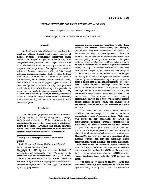
AIAA-98-1779 NEURAL NETWORKS FOR RAPID DESIGN AND ANALYSISDean W. Sparks, Jr.* and Peiman G. MaghamiNASA Langley Research Center, Hampton, VA 23681-0001AbstractArtificial neural networks have been employed for rapid and efficient dynamics and control analysis of flexible systems. Specifically, feedforward neural networks are designed to approximate nonlinear dynamic components over prescribed input ranges, and are used in simulations as a means to speed up the overall time response analysis process. To capture the recursive nature of dynamic components with artificial neural networks, recurrent networks, which use state feedback with the appropriate number of time delays, as inputs to the networks, are employed. Once properly trained, neural networks can give very good approximations to nonlinear dynamic components, and by their judicious use in simulations, allow the analyst the potential to speed up the analysis process considerably. To illustrate this potential speed up, an existing simulation model of a spacecraft reaction wheel system is executed, first conventionally, and then with an artificial neural network in place.I ntroductionThe overall design process for aerospace systems typically consists of the following steps: design, analysis and evaluation. If the evaluation is not satisfactory, the process is repeated until a satisfactory design is obtained. Dynamics and control analyses, which define the critical performance of many aerospace systems, are particularly important. Generally, all_____________________________* Aerospace Technologist, Guidance and Control Branch.Senior Research Engineer, Guidance and Control Branch, Senior Member, AIAA.Copyright Ó 1998 by the American Institute of Aeronautics and Astronautics, Inc. No copyright is asserted in the United States under Title 17, U.S. Code. The U.S. Government has a royalty-free license to exercise all rights under the copyright claimed herein for Governmental purposes. All other rights are reserved by the copyright owner.aerospace systems experience excitations resulting from internal and external disturbances, for example, aerodynamic turbulence encountered by aircraft or instrument scanning in space systems. Excessive vibrations due to turbulent aerodynamics could diminish the ride quality or safety of an aircraft. In space systems, excessive vibrations could be detrimental to its science instruments which usually require consistently steady pointing in a specified direction for a prescribed time duration. Typically, in the course of the design of an aerospace system, as the definitions and the designs of the system and its components mature, several detailed dynamics and controls analyses are performed in order to insure that all mission requirements are being met. These analyses, although necessary, have historically been very time consuming and costly due to the large number of disturbance scenarios involved, and the extent of time domain simulations that need to be carried out. For example, a typical pointing performance analysis for a space system might require several months or more, which can amount to a considerable drain on the time and resources of a space mission.It is anticipated that artificial neural networks (ANNs) can be used to significantly speed up the design and analysis process of aerospace systems. This paper will focus on the application of ANNs in approximating nonlinear dynamic components in simulations, in order to reduce overall time domain analysis time and compute effort. Initial work has shown that ANNs, once properly trained, can be used in place of nonlinear dynamical systems in simulations. These ANNs can give very good approximations of the systemsÕ outputs, and they can drastically reduce computational burden in running the overall simulation.A numerical example of a dynamical system simulation with an ANN is presented, and comparisons between conventional (i.e., without the ANN) simulation times, in terms of computer processing unit (CPU) seconds, versus simulation times with the ANN in place is made.The paper is organized as follows. After this introduction section, a brief description on conventional dynamics analysis is given. Next, discussions onneural networks, their use in approximating functional relationships, together with a typical design outline, is presented. Then, numerical results of an example application of an ANN in a simulation is reported. Finally, a conclusions section closes the paper.Conventional Dynamics AnalysisConventional dynamics analysis can be divided into two categories: time domain analysis and frequency domain analysis. Both are used to determine specific characteristics of a system performance, but as implied by their respective names, the characteristics are either defined in terms of time or as a function of frequency. In this paper, the emphasis will be on time domain analysis. Time domain analysis tries to compute the transient and steady state time responses of a system given specific inputs. Examples of typical system response characteristics, which are studied in time domain analysis, include transient system response maximum overshoot, rise and settling times. Another is the systemÕs steady state performance, which is usually defined by some metric on the steady state error between the system response and a reference signal. If the system is simple enough, i.e., linear, of very low order and has relatively few inputs and outputs, like a single-input, single-output (SISO) system, its responses can be obtained by direct solution of the system equations which describe the model. However, most realistic system models are of high order and/or nonlinear, which precludes a direct solution. The usual procedure in this case is to construct a simulation of the system to obtain the time responses, via integration (e.g., Runge-Kutta methods) of the systemÕs equations of motion. There are available several simulation-based packages, such as MATRIXx/System Build and MATLAB/Simulink, which can perform whatever time domain analysis is required. However, even with these tools, computing time response solutions can be expensive both in terms of time and effort, depending upon a number of factors, such as the order of the system, the number of inputs and outputs, the level of nonlinearities, the type and level of disturbance inputs and/or reference signals, and the kind of integration selected.Whatever type of analyses need to be done, it would be highly beneficial to the analyst to be able to rapidly assess the effects on system time response performance due to the almost inevitable design changes that a system will undergo during its lifetime. During the design phase of an aerospace system, almost all components go through some level of change, with each change having the potential to affect the performance of the overall system to some degree. In many instances, these changes are expected to affect the performance of the system to such a degree as to warrant a partial or full analysis of its performance. In the area of spacecraft dynamics and controls, these types of changes include: changes in the inertia or flexibility of the structural components which would affect the dynamic characteristics of the spacecraft; changes in the characteristics of the external and internal disturbances that may act on the spacecraft while it is in orbit; or changes in the control system design, hardware, and software. For example, for a reaction wheel system, changes could include: wheel size, nonlinear friction characteristics, or wheel speed internal controller design. Now, depending on the nature and extent of these changes, there may be a need to reevaluate the controlled dynamical responses of the system. The computational time and cost associated with each of these performance analyses (i.e., executing conventional time simulations) may be substantial. The cost can be exorbitant especially if the analysis has to be repeated several times during the design phase. One approach to this problem is to use artificial neural networks (ANNs) to help speed up the analysis.Rapid Analysis with ANNsThe motivation behind the use of ANNs is to speed up the analysis process substantially. The main use of ANNs lies with their ability to approximate functional relationships, specifically nonlinear relationships. This can be either a static relationship, one that does not involve time explicitly, or a dynamic relationship, which explicitly does involve time. Dynamic approximations via ANNs can be achieved by using the appropriate time delays and feedback of the output back to the input, which is defined as recurrence. Such networks are referred to as recurrent networks1,2. In any case, to an ANN, there is no distinction between a static or dynamic map, there is just input/output data. For example, an ANN could be designed to approximate the dynamic behavior of a nonlinear component, e.g., the mapping between the nonlinear torque output of a spacecraft reaction wheel and its angular wheel speed and input torque command. Once such a network is trained, the torque output of the wheel, for given wheel speed and torque command inputs, can be easily obtained by simulating the ANN. One application of ANNs is to use them to speed up the simulation process and therefore, the overall analysis time. For example, ANNs can be designed to approximate the outputs of a continuous-time, nonlinear system, with outputs computed for a specified discrete step. This way, thetraditional continuous-time integration (e.g. Runge-Kutta) of the nonlinear dynamics can be replaced by discrete-time nonlinear algebraic updates, with reasonable accuracy. Although the initial training time for an ANN may be long, it can be performed during off hours, in a semi-automated manner, without much direct involvement by the designer. Also, once an ANN has been designed to represent a dynamic component, it can be stored in a component library and recalled for use in future analyses.The successful design of an ANN depends on the proper training of the network. The training of a network involves the judicious selection of points in the input variable space, which along with the corresponding output points, constitute the training set. In the reaction wheel example, in order to properly train an ANN approximation, it is important that the input points, i.e., the wheel speed and commanded torque values, completely cover the range of possible values for both. In addition, it is important that enough points are selected such that they cover areas where fine resolution in the design space is required, i.e., areas where small variations in input data cause large variations in the corresponding output data. Of course, there will be the inevitable trade-off between selecting enough points for good training and keeping the number of training points down to practical levels for computation.Before proceeding, it is important to restate here that the true advantage of using ANNs lies with modeling nonlinear relationships. Although one can certainly use ANNs to represent linear systems, there will be no gain, in terms of reductions in compute time and effort, in their use over conventional representations of the same linear systems. One can always take any pure linear, dynamical system and rewrite it as a series of output difference equations, which are functions of appropriate time-delayed output feedbacks and input signals. It turns out that the coefficients of these system output equations are equivalent to the Òweighting coefficientsÓ (which are defined in the following subsection) of pure linear ANNs, with the ÒbiasÓ parameters (see following subsection) set to zeros. Thus, there would be no point in training ANNs to represent linear dynamical systems. Therefore, the work reported in this paper will only cover representing nonlinear systems with ANNs.In the following subsections, a brief overview of ANNs and the training of a specific type of ANN that was used in this work, are presented.Artificial Neural Networks (ANNs)Artificial neural networks (ANNs) have grown into a large field since their inception, and a complete discussion on them is beyond the scope of this paper. Instead, this section will present a very brief description on ANNs. ANNs were developed as an attempt to mimic the process of the human brain. They consist of groups of elements (called neurons) which perform specific computations on incoming data, with interconnections which permit data flow from one group of neurons to the next, similar to the way groups of biological neurons receive and transmit information through dendrites and axons, respectively, in a brain. Like their biological counterparts, ANNs can be trained to perform a variety of tasks, such as modeling functional relationships. The parameters of the ANN, when presented with the appropriate input and output data related to a specific functional relationship, can be adjusted such that the ANN can give a good representation of that relationship. This feature is particularly useful when the relationship is nonlinear and/or not well defined, and thus difficult to model by conventional means. Also ANNs, by their very nature, are a perfect fit for efficient parallel computations on digital computers. Though there are several types of ANNs, in this paper, only the feedforward ANN will be discussed.A typical feedforward ANN is depicted in Figure 1, with m inputs and npoutputs, and eachInputLayerHiddenLayer 1HiddenLayer 2OutputLayerinput 1input 2input moutput 1output 2n p Figure 1. Typical feedforward ANN. circle, or node, representing a single neuron. The name feedforward implies that the data flow is one way (forward) and there are no feedback paths between neurons. The output of each neuron from one column is an input to each neuron of the next column. Using the typical naming convention, each column of neurons is called a layer, the initial column where the inputs come into the ANN is called the input layer, and the last layer, i.e., where the outputs come out of the ANN, is denoted as the output layer. All other layers in between are called hidden layers. These ANNs can have as many layers as desired, and each hidden layer can haveas many neurons as desired. Each neuron can be modeled as shown in Figure 2, with n being the number of inputs to the neuron.output from neuronto Figure 2. Representation of a neuron in the feedforwardANN.Associated with each of the ninputs is some adjustable scalar weight, w i , i= 1, 2, ..., n , which multiplies that input. In addition, an adjustable bias value, b, can be added to the summed scaled inputs. These combined inputs arethen fed into an activation function, which produces the output of the neuron. The activation function can take on many forms to shape the output;three of the more common functions are linear, tan sigmoid, and log sigmoid, as shown in Figure 3. Thelinear activation function simply outputs the input; the tan sigmoid function is the hyperbolic tangent function,with output values between [-1,1] for inputs (-¥,+¥);while the log sigmoid is also a nonlinear function,which can be written as y e x=+-11/(), with the outputs values, y , in the range [0,1], given inputs, x , in the range (-¥,+¥). During training, the set of weights and bias terms associated with the neurons are adjusted until the output of the ANN matches, to within some specified level of tolerance, the true outputs for the same inputs.The objective is to design a feedforward network to map the functional relationship between a set of input points and a corresponding set of output points, or target points. To accomplish this task, a feedforward network, like the one shown in Figure 1, but with only one hidden layer, is considered. The input layer has n cnodes, corresponding to the elements of the input vector, while the output layer has n p nodes, which correspond to the elements in the output vector. The number of nodes in the hidden layer is arbitrary,however, it has to be large enough to guarantee convergence of the network to the functional relationship that it is to approximate. Once the number of nodes in the hidden layer has been chosen, the network design is reduced to adjusting, or training, the weighting coefficients and biases. The parameters of feedforward networks are usually trained using either a gradient method named the back propagation method 1,2,or a pseudo-Newtonian approach, such as the Levenberg-Marquardt 3 technique. Typically, in these methods, the weights and biases are trained to minimize some cost function of the error of the network. The network error is defined as the difference between the output of the true system and that of its ANN approximation, for a given set of inputs. The cost function is usually taken as the sum squared error of the network over all of the input points. If q sets of points (e.g., points taken for q time samples) are used for training the network, then the input U to the network would be an n c x q matrix, with each column corresponding to a set of input points for a given time sample, and the output Y p would be a n c x q matrix,with each column of Y p corresponding to that of U .Now the cost function, in terms of the sum squared error of the network, can be written asE e k Y j r Y j r d p j n r qk qn pp==-===ååå()((,)(,))22111(1)where Y d is a n p x q matrix of the target outputs. The typical procedure is to keep updating the weights and biases until the error E goes below some specified tolerance level. At this point, the feedforward network is considered trained.It has been shown in the literature that a feedforward network with only one hidden layer can approximate a continuous function to any degree of accuracy 4-6. It is obvious that this capability carries over to networks with more than one hidden layer. The use of feedforward ANNs has some advantages over the conventional approximation techniques, such as polynomials and splines. For example, polynomials are hard to implement in hardware due to signal saturation, and if they are of higher order, there may be stability problems in determining the coefficients.ANNs, on the other hand, are very amenable to hardware implementation. As a matter of fact, to date, several VLSI chips based on multilayer neural network architecture are available 7,8.Reaction Wheel Model ExampleIn order to illustrate the feasibility of using ANNsto approximate dynamic components, a model of a reaction wheel assembly, consisting of three reaction wheels, one each for the roll, pitch, and yaw axes of a spacecraft, was selected as a test application. Figure 4shows the blockrepresentation of a reaction wheel model in this assembly; this model was used for all three wheels.This model is fairly simple in nature, and consists of the following: the input, T com , is the torque command (in units of N-m) to the reaction wheel, which is updated every 1.024 seconds; T act , in N-m, is the actual torque output of the wheel, which includes nonlinear viscous friction torque; the wheel momentum, M w ; and the angular wheel speed, W sp , which is converted into units of revolutions per minute (RPM). The parameter J w is the wheel inertia. The actual torque output of the wheel, T act , is the combination of the torque command and viscous friction torque, T fric , (which takes the opposite sign of that of the wheel speed W sp ): T T T sign W actcom fric sp =-*(). (2)Two different nonlinear functions were used to model the wheel friction torque: a quadratic function in terms of wheel speed; and an exponential function in terms of wheel speed. In each case, an ANN was designed to approximate the dynamics of the wheel.The results are presented in the following subsections. Quadratic Friction FunctionIn the first case, the wheel viscous friction torque was modeled with a quadratic function in terms of W sp ,which is given below:T awaw aw W fric sp =+=--33671761024104510562.*.*,x x . (3)The above wheel model is continuous and nonlinear, and in the past, has been simulated using aRunge-Kutta (2,3) variable step size integration for accurate, but time consuming, integration. The error tolerance for the integration was set at 10-6, the minimum step size set at 10-8 seconds, and the maximum step size at one time sample of 1.024seconds. Note that the tight error tolerance was required for solution accuracy. One way to speed up the simulation was to convert the continuous-time model into a discrete-time model, and then use discrete updates at every 1.024 seconds to propagate the system state equations. However, as will be discussed later in this section, the direct discrete simulation of this model results in unacceptable inaccuracies because of the nonlinear torque friction component.To try to keep the speed advantage of discrete update simulations, and still maintain reasonable accuracy in the wheel model outputs, an ANN was trained to map the functional relationship from the torque input command at the k th discrete time step,T com (k), and wheel speed at the k th time step, W sp (k), to the wheel speed for the next time step, W sp (k+1). In other words, the wheel speed from one time step to the next was approximated. Figure 5 depicts the discrete-time model of the reaction wheel, with a single-hidden layer ANN (hidden layer with a tan sigmoid activation function, the output layer with a pure linear function)computing W sp (k+1). A unit delay is in place to obtain the current (k th step) wheel speed.The friction torque computation was done the same way as in Figure 4. It was felt that there would be no real advantage gained in substituting a separate ANN to replace the simple quadratic friction function (Eq. 2),which was a static map. Since the same model was used for each of the three wheels in the assembly, the same ANN could be used for each wheel.Before the ANN for the wheel speed could be trained, the appropriate input/output training data had to be generated. To accomplish this, proper data points for both the torque command T com and wheel speed W sp ,the two inputs to the ANN, had to be selected first.With this specific wheel model, the expected operating range for T com was assumed to be +/- 0.1 N-m, and +/-300 RPM for Wsp. To get adequate coverage of datapoints over these ranges, the Tcompoints were taken inequally-spaced increments of 0.005 N-m, while the Wsp points were taken in increments of 3.0 RPM. With these ranges and increments, the total number oftraining input pairs (Tcom , Wsp) was 8,241. Thecorresponding training output, or target, points werethen computed by taking each training input pair, and running a MATLAB (v5.0)/Simulink (v2.0) simulation of the continuous reaction wheel model (Figure 4) over a specified time interval [0, Tstep]; the wheel speed valueat time Tstepwas recorded as the desired target point for that specific training pair. As mentioned earlier, forthis reaction wheel model, Tstepwas set to 1.024 seconds. Each Simulink simulation used the second-order, three-function-evaluation-per-step Bogaki-Shampine variable-step integration routine, the minimum and maximum step sizes allowed were set at 10-8 and 1.024 seconds, respectively; the relative and absolute error tolerance parameters were set to 10-6.Each Tcominput value was held constant over the integration range [0, 1.024], while the correspondingWspinput value was entered as the initial wheel speed value (i.e., at time 0) in the pure integrator block.After the training data was generated, the ANN could now be trained. Prior to the actual ANN training, both the input and output training data were normalized with respect to their absolute maximum values; by keeping the training data in the [-1, 1] range, more efficient use of the ANN training routines was obtained. The training led to a feedforward ANN with one 10-neuron, hidden layer (using a tan sigmoid activation function) and a pure linear output layer. The training was performed using the standard ÔtrainlmÕ function from the MATLAB Neural Network Toolbox, which is based on the Levenberg-Marquardt training algorithm [Ref. 3]. Running on a Sun Ultra-2 Workstation, the training of this ANN completed in less than 2.0 (elapsed time) hours. The training reduced the sum squared error (see Eq. (1)) of the ANN down to a level of 2.98 x 10⁻⁵, which was deemed acceptable. Once the training was completed, the final ANN weights and bias numbers were scaled back to their true values. In checking the accuracy of the approximation achieved by this ANN, given the training input points, the mean percent error between the true target points and the ANN outputs points was 0.063% , and only 1.07% of the points had errors greater than 1%.Once the ANN-based model of the reaction wheel assembly was developed, its performance, in terms of accuracy and execution CPU time, was evaluated in several discrete-time simulations under a specific set oftorque command input, Tcom, profiles. These 6000-second torque command profiles for the roll, pitch and yaw axis wheels, respectively, shown in Figure 6, werea series of 1.024-second-wide pulses. In addition, a small random signal was added to the pitch axis wheel torque command. These could be typical torquecommand profiles required to counter the motions of Figure 6. Roll, pitch and yaw torque input commandprofiles.scanning instruments on a spacecraft, for example. The original continuous-time reaction wheel assembly model, as shown in Figure 4, was also simulated using the Simulink second-order, three-function-evaluation-per-step Bogaki-Shampine variable-step integration routine, with the minimum and maximum step sizes allowed were set at 10-8 and 1.024 seconds, respectively. The relative and absolute error tolerance parameters were set to 10-6. The results of this simulation were considered the ÔtrueÕ results, against which the other simulations were tested. The average execution time for this Ôtrue modelÕ simulation was 15.01 CPU seconds on the Sun Ultra-2.Using the ANN-based model of the reaction wheel assembly, two different discrete-time simulations, both running at a discrete update period of 1.024 seconds, were performed to see if meaningful reductions in simulation execution times can be achieved without sacrificing accuracy down to unacceptable levels. Table 1 contains the execution times (in CPU seconds), the rms and maximum absolute errors (as compared to the Ôtrue modelÕ results from above) for three discrete-time simulations . First, a MATLAB function file version of the ANN-based discrete-time model was written; this function was executed in MATLAB v5.0. The average execution time for was 6.49 CPU seconds. In comparing the wheel speed outputs from this discrete function file simulation with those from the Ôtrue modelÕ, very good agreement was observed; theTable 1. Discrete-time simulation results for quadratic friction case.Simulation C P Usecrmserror(RPM)Max.error(RPM)ANN MATLAB functionroll axis wheelpitch axis wheelyaw axis wheel 6.490.00110.00490.02630.00920.07900.0417ANN MEX fileroll axis wheelpitch axis wheelyaw axis wheel 0.350.00110.00490.02630.00920.07900.0417discrete MATLAB functionroll axis wheelpitch axis wheelyaw axis wheel 1.711.84371.39684.291541.568380.603763.6718root-mean-square (rms) of the errors between ÔtrueÕ and ANN-based discrete-time simulation outputs, over the length of the simulation, were 0.0011 RPM for the roll axis wheel, 0.0049 RPM for the pitch axis wheel, and 0.0263 RPM for the yaw axis wheel. These results indicated that, although acceptable simulation accuracies were achieved with the ANN-based model, the execution time speed up was only a factor of 2.3.This was somewhat expected, because the friction nonlinearity was fairly benign, i.e., the Runge-Kutta integration did not have to take many steps to converge to the solution. More reduction in execution time can be achieved if another compute language is used, one with faster loop execution capability. To do this, the ANN-based wheel model simulation was written in FORTRAN-77, for execution as a MEX file called by MATLAB. MEX files are dynamically linked subroutines which MATLAB can load and execute like regular MATLAB functions.The third simulation was just a pure discrete-time simulation (zero-order-hold integration, with no ANN) of the wheel assembly, sampled at 1.024 seconds. This simulation was also written as a MATLAB function, and executed in MATLAB v5.0.The results in Table 1 show that although the pure discrete wheel model simulation executes at a faster rate, its accuracy leaves much to be desired. Figure 7. shows the roll axis wheel speed output time histories for this case, from the Ôtrue modelÕ Simulink simulation (top), from the ANN-based model MEX file simulation (middle), and the pure discrete-time model simulation (bottom). In these simulations, the initial angular speed of all three wheels was 250 RPM.Figure 7. Roll axis wheel speed simulation results. Clearly, the ANN-based MEX file simulation results matched the Ôtrue modelÕ results much better than did the pure discrete-time simulation results. The combination of the nonlinearity and the rapid dynamics caused by the pulse command profile made it difficult for the pure discrete model to accurately match the Ôtrue modelÕ simulation, at the update period of 1.024 seconds. On the other hand, the ANN-based wheel model simulations, while executing slower than the pure discrete model simulation, gave much more accurate results. The ANN-based wheel model MEX file simulation gave wheel output results which were very comparable to the Ôtrue modelÕ results, while executing about 40 times faster, which was a fairly significant speed up.Exponential Friction FunctionIn the second case, the wheel viscous friction torque was modeled with an exponential function in terms of Wsp, which is given below:T aw e aw Wfricawsp==-001001.**,.. (4)As in the quadratic friction function case, an ANN-based model of the reaction wheel assembly was designed. Another 10-node, feedforward ANN, was trained in the exact manner as reported in the previous case. Running on the Sun Ultra-2 Workstation, the training of this ANN completed in less than 2.0 (elapsed time) hours. The training reduced the sum squared error of this ANN down to 3.009 x 10⁻⁴, which was deemed acceptable. In checking the accuracy of this ANN, given the training input points, the percent error between the true target points and the ANN outputs points were 0.419% on average, and only 1.32% of the。
人工智能算法辅助药物分子设计及优化方法探究
人工智能算法辅助药物分子设计及优化方法探究随着科技的飞速发展,人工智能(Artificial Intelligence,AI)在药物研发领域扮演着愈发重要的角色。
人工智能算法的引入为药物分子设计和优化带来了新的可能性和机遇。
本文将探究人工智能算法在药物分子设计和优化中的应用,进一步探讨其优势和挑战。
药物分子设计和优化是一项繁琐而复杂的任务,需要大量的时间和资源。
而且,许多候选化合物往往在实验过程中无法通过安全性和有效性的测试。
这就需要寻找一种更高效和准确的方法来筛选和设计出具备药物活性的化合物。
人工智能算法通过利用机器学习和数据分析的技术,可以处理大规模的分子数据和化学信息。
AI模型可以通过训练大量的化合物数据,以理解化合物的结构-性能关系。
这样,AI模型可以通过预测和评估化合物的属性和药物活性,从而为药物设计提供指导。
首先,人工智能算法能够帮助药物分子的快速筛选。
传统的方法往往需要依赖人工经验和实验室测试。
而人工智能算法可以通过模型的训练和学习,识别潜在的药物候选化合物。
这一过程可以减少大量的实验工作,节省时间和资源。
其次,人工智能算法能够加快药物分子的优化过程。
药物的优化通常需要对分子结构进行修改和调整,以提高其活性和选择性。
人工智能算法可以通过分子模拟和计算预测,评估不同分子结构的性能。
这样,研究人员可以更快地找到最佳的化合物结构,节约了大量的试错过程。
另外,人工智能算法在药物分子设计中还能辅助寻找新的药物靶点。
通过分析疾病相关的基因、蛋白质和代谢途径等信息,AI模型可以发现新的潜在靶点,并提供相应的候选化合物。
这种方法有助于加速新药物的发现进程,为药物行业的创新提供了巨大的机遇。
然而,人工智能算法在药物分子设计和优化中也面临一些挑战。
首先是数据质量问题。
AI模型需要大量的高质量数据来进行训练和学习,但往往存在数据的不一致性和不完整性。
因此,在构建AI模型之前,收集和处理数据需要非常慎重。
药物发现与设计的计算方法

药物发现与设计的计算方法药物发现与设计是现代医药领域中非常重要的一项工作。
它涉及到药物的发现、设计和优化等方面,通过计算方法来加速药物研发的过程。
本文将介绍药物发现与设计中常用的计算方法及其应用。
一、分子模拟分子模拟是药物发现与设计中常用的计算方法之一。
它可以通过计算机模拟药物分子与靶标分子之间的结合方式,预测药物分子的活性和亲和力。
分子模拟可以帮助研究人员设计出具有高活性的药物分子,并降低实验成本和时间。
分子模拟主要包括分子对接和药物动力学模拟两个方面。
分子对接是通过计算机模拟药物和靶标之间的相互作用,寻找最佳的药物分子结构。
药物动力学模拟则可以模拟药物在生物体内的行为,比如血药浓度的变化和药物代谢情况。
二、药效团建模药效团建模是一种通过分析已知活性化合物的共同特征来预测其他潜在活性化合物的计算方法。
它主要通过筛选已知的活性分子数据库,并通过计算和分析这些化合物的特征,识别出影响其活性的各种因素。
然后根据这些特征,设计新的分子结构,从而发现具有更高活性的药物分子。
药效团建模常用的方法包括药效团筛选和定量构效关系(QSAR)模型。
药效团筛选通过识别化合物中的活性团或基团,挖掘出具有活性的共同特征。
而QSAR模型是通过建立活性化合物与其生物活性之间的定量关系模型,来预测新的化合物的生物活性。
三、虚拟筛选虚拟筛选是一种通过计算方法筛选大规模化合物库,预测其与靶标的相互作用,从而快速找出具有潜在活性的药物候选分子。
虚拟筛选可以大大减少实验筛选的范围,提高药物研发的效率。
虚拟筛选常用的方法包括构建药物化学特征数据库和基于结构的筛选。
通过构建药物化学特征数据库,将化合物按照相关特征进行分类和存储,并结合已有的活性化合物信息,筛选出具有潜在活性的化合物。
基于结构的筛选则是通过计算和模拟化合物的结构,与靶标分子之间的相互作用,预测其活性。
四、计算辅助合成药物发现与设计中的计算辅助合成是一种通过计算方法辅助研究人员设计合成路线和优化化学方法的技术。
基于脑-机接口和嗅觉解码的仿生气味识别系统

基于脑-机接口和嗅觉解码的仿生气味识别系统董琪;秦臻;胡靓;庄柳静;张斌;王平【摘要】Mammalian olfactory systems have merits of higher sensitivity, selectivity and faster response than current electronic nose systems based on chemical sensor array in odor recognition. The purpose of this study is to develop a biomimetic olfactory sensing system based on brain-machine interface technology for odor detection in vivo electrophysiological measurements of olfactory bulb. In this work, extracellular potentials of mitral/tufted cells in olfactory bulb were recorded by implanted 16-channel microwire electrode arrays. The odor-evoked response signals were analyzed. We found that neural activities of different neurons showed visible different firing patterns in both temporal features and rate features when stimulated by different small molecular odorants. Odors were classified by an algorithm based on population vector similarity and support vector machine. The results suggest that the novel bioelectonic nose is sensitive to odorant stimuli. With the development of BMI and olfactory decoding methods, we believe that this system will represent emerging and promising platforms for wide applications in medical diagnosis and security fields.%为了探讨利用生物嗅觉传感系统进行气味识别的可行性,提出了一种基于脑-机接口的仿生气味识别系统。
化学模拟的新方法博士生在计算化学领域的突破
化学模拟的新方法博士生在计算化学领域的突破随着科技的不断进步和发展,计算化学作为一门交叉学科,在研究和应用领域都取得了长足的发展。
作为计算化学领域的一项重要技术,化学模拟在化学分子结构与物性关系研究、反应机理研究、新材料设计等领域中发挥着重要的作用。
近年来,博士生们在计算化学领域做出了一系列突破性的工作,提出了一些新的方法和技术,为化学模拟的发展带来了新的机遇和挑战。
一、基于量子力学的化学模拟方法1. 密度泛函理论(DFT):DFT是计算化学领域中广泛应用的一种方法,可以精确地描述分子的几何结构和电子性质。
博士生们通过改进密度泛函的选择和开发新的近似方法,进一步提高了DFT的预测能力和计算效率。
2. 含时密度泛函理论(TDDFT):TDDFT将密度泛函理论扩展到含时情况下,可用于研究分子的激发态和光谱性质。
博士生们提出了一些新的TDDFT方法,例如自洽场TDDFT和线性响应TDDFT,并成功地应用于材料科学和光化学领域。
二、经典分子动力学模拟方法1. 分子力场模拟:分子力场模拟利用经典力场来计算分子系统的能量和结构,可以预测分子的构象和动力学行为。
博士生们通过参数化力场和优化模型,提高了分子力场模拟的准确性和可靠性。
2. 相关动力学模拟:相关动力学模拟基于统计力学原理,通过模拟原子与周围环境之间的相互作用来预测分子的运动和相变行为。
博士生们开发了一些新的相关动力学方法,如Path Integral Molecular Dynamics (PIMD),辅助了理论化学的研究与进展。
三、机器学习方法在化学模拟中的应用近年来,机器学习技术的发展给化学模拟带来了新的思路和方法。
博士生们利用机器学习算法,通过大量的计算和实验数据,构建了预测模型,用于高通量筛选材料和预测化学反应的产物。
这些方法不仅提高了计算效率,还在新材料的探索和设计中发挥了关键作用。
总结:博士生们在计算化学领域的研究中,通过提出新的方法和改进已有方法,推动了化学模拟技术的发展。
人工智能在化学或药学领域应用的文献

人工智能在化学或药学领域应用的文献人工智能在化学和药学领域的应用文献非常丰富。
人工智能技术如机器学习、深度学习和自然语言处理等已经被广泛应用于分子设计、药物发现、材料科学以及化学反应预测和优化等方面。
以下是一些代表性的研究文献。
1. Gómez-Bombarelli等(2016)提出了一种可以自动进行化学反应设计和优化的方法,采用了深度学习算法。
该算法利用了大量的实验数据和计算结果,能够预测分子的性质并生成具有特定性质的分子。
这一方法在有机合成的中间体设计和催化剂的发现方面具有重要应用。
2. Segler等(2018)提出了一种基于循环神经网络的生成模型,用于预测有机分子的化学反应路径。
该模型可以根据给定的起始分子和目标分子,生成一系列合成步骤,以实现目标分子的合成。
这一方法在药物合成和有机合成中具有很大的潜力,能够加速新药物的开发过程。
3. Schneider等(2019)发展了一种基于机器学习的方法,用于预测有机反应的副反应。
该方法利用了大量的实验数据和反应条件参数,能够准确地预测有机反应中可能发生的副反应,从而为反应优化和副反应控制提供了重要的指导。
4. Olivecrona等(2017)开发了一种基于深度学习的方法,用于预测小分子的生物活性。
该模型可以根据分子的结构和属性,准确地预测分子与目标蛋白的结合亲和力。
这一方法在药物发现和虚拟筛选中具有重要的应用价值。
5. Gomez-Bombarelli等(2018)利用深度生成模型和强化学习算法,开发了一种新的药物发现方法。
这种方法能够通过迭代学习,自动设计出新的多靶点药物,减少筛选和合成的时间和成本。
除了以上几篇研究论文外,还有许多关于人工智能在化学和药学领域应用的文献。
这些研究表明,人工智能技术在化学和药学领域具有广阔的应用前景,可以加速药物发现过程,降低合成成本,提高合成效率,并为有机合成反应和药物设计提供重要的指导。
然而,人工智能在化学和药学领域的应用也面临一些挑战,如数据质量问题、算法的可解释性和可靠性等。
中国帕金森病的诊断标准

中国帕金森病的诊断标准(2016版): 268-271. DOI: 帕金森病(Parkinson's disease)是一种常见的神经系统退行性疾病,在我国65岁以上人群的患病率为1 700/10万,并随年龄增长而升高,给家庭和社会带来沉重的负担[]。
该病的主要病理改变为黑质致密部多巴胺能神经元丢失和路易小体形成,其主要生化改变为纹状体区多巴胺递质降低,临床症状包括静止性震颤、肌强直、运动迟缓和姿势平衡障碍的运动症状[]及嗅觉减退、快动眼期睡眠行为异常、便秘和抑郁等非运动症状[]。
近10年来,国内外对帕金森病的病理和病理生理、临床表现、诊断技术等方面有了更深入、全面的认识。
为了更好地规范我国临床医师对帕金森病的诊断和鉴别诊断,我们在英国UK 脑库帕金森病临床诊断标准的基础上,参考了国际运动障碍学会(MDS)2015年推出的帕金森病临床诊断新标准,结合我国的实际,对我国2006年版的帕金森病诊断标准[]进行了更新。
一、帕金森综合征(Parkinsonism)的诊断标准帕金森综合征诊断的确立是诊断帕金森病的先决条件。
诊断帕金森综合征基于3个核心运动症状,即必备运动迟缓和至少存在静止性震颤或肌强直2项症状的1项,上述症状必须是显而易见的,且与其他干扰因素无关[]。
对所有核心运动症状的检查必须按照统一帕金森病评估量表(UPDRS)中所描述的方法进行[]。
值得注意的是,MDS-UPDRS仅能作为评估病情的手段,不能单纯地通过该量表中各项的分值来界定帕金森综合征。
二、帕金森综合征的核心运动症状1.运动迟缓:即运动缓慢和在持续运动中运动幅度或速度的下降(或者逐渐出现迟疑、犹豫或暂停)。
该项可通过MDS-UPDRS中手指敲击()、手部运动()、旋前-旋后运动()、脚趾敲击()和足部拍打()来评定。
在可以出现运动迟缓症状的各个部位(包括发声、面部、步态、中轴、四肢)中,肢体运动迟缓是确立帕金森综合征诊断所必需的。
基于最小二乘法的改进的随机椭圆检测算法

第42卷第8期2008年8月浙 江 大 学 学 报(工学版)Journal of Zhejiang University(Engineer ing Science)Vol.42No.8Aug.2008收稿日期:2007205218.浙江大学学报(工学版)网址:/eng基金项目:宁波市科技计划资助项目(2006B100027).作者简介:陈海峰(1982-),男,浙江台州人,硕士生,从事数字图像处理工作.E 2mail:optical.dlz@通讯联系人:冯华君,男,教授,博导.E 2mail:fen ghj@DOI:10.3785/j.issn.10082973X.2008.08.015基于最小二乘法的改进的随机椭圆检测算法陈海峰1,雷 华1,孔燕波2,周柳云2,冯华君1(1.浙江大学现代光学仪器国家重点实验室,浙江杭州310027;2.宁波华光精密仪器有限公司,浙江宁波315153)摘 要:为了提高数字图像中椭圆检测的效率和准确性,提出了一个基于最小二乘法的改进的随机椭圆检测算法.该算法随机选取图像中的3个边缘点,在以这3个点为中心的窗口内,从边缘点中拟合出可能椭圆,并通过随机选取的第4个边缘点来确认可能椭圆.利用直接最小二乘法椭圆拟合的特性,引入可能椭圆边缘点收集和椭圆重新拟合的迭代过程来提取最终的椭圆参数.通过对含有不同噪声的仿真图片和包括残缺椭圆的实际图片的实验表明,新算法的改进是有效的.与原算法相比,新算法降低了对参数的依赖性,提高了检测的速度、稳定性和准确性,同时保留了原算法的抗噪声能力.关键词:椭圆检测;随机检测;最小二乘法中图分类号:T P391 文献标识码:A 文章编号:10082973X(2008)0821360205An improved randomized algorithm for detecting ellipsesbased on least square approachCH EN Hai 2feng 1,LEI H ua 1,KONG Yan 2bo 2,ZHOU Liu 2yun 2,FENG Hua 2jun 1(1.State Key Labor a tory of Moder n Optica l I nstr umentation ,Zhej ia ng Univer sity,H a ngz hou 310027,China ;2.H ua guang P recision I nstr ument Co.Ltd.,N ingbo 315153,China)Abstr act:An improved randomized ellipse detection algorithm based on least square approach was proposed to enhance the efficiency and accuracy of ellipse detection in digital images.T his algorithm r andomly se 2lects three edge points in the image,and then uses least squar e approach to fit all the edge points in three windows,which are defined by the three edge points.T he forth edge point is randomly selected to judge whether a possible ellipse exists in the image.Utilizing the char acteristic of direct least square fitting of ellipse,an iteration process of edge point collecting and ellipse refitting of possible ellipse was introduced to extract the final ellipse .s parameters.A rtificial images with different levels of noise and nature images containing incomplete ellipses were employed to test this algor ithm.Experimental results show that the impr ovements are pared with the original algorithm,the proposed algorithm reduces the de 2pendence on arguments of detection algorithm,and enhances the speed,stability and accuracy of ellipse de 2tection,while preserves the anti 2noise ability of the original algorithm.Key words:ellipse detection;randomized detection;least square approach 椭圆检测在模式识别领域一直是研究的热点.在过去的20多年中,人们提出了很多椭圆检测算法.例如:基于H ough 变换及其改进算法的椭圆检测算法、最小二乘拟合算法、基于随机抽样一致性(random sample consensus,RA NSA C)思想的算法、遗传算法以及结合椭圆几何特性的算法.这些算法大致可以分为投票(类聚)和最优化2大类.H ough变换、RANSAC算法都是采用映射的方法,将样本点映射到参数空间,采用累加器或者类聚的方法来检测椭圆.这类算法具有很好的健壮性,能够一次检测多个椭圆,但是需要复杂的运算和大量的存储空间.最优化方法包括最小二乘拟合算法、遗传算法以及其他最优化椭圆拟合方法.这类方法的主要特点在于准确性高,但是通常需要预先进行分割或分组处理,无法直接用于多个椭圆的检测,对噪声的敏感程度高于前一类方法.近年来,人们对椭圆检测的研究大多在数据点收集、椭圆真伪的验证和各类方法相互结合的方向上展开.Cheng等人[1]提出的受限随机Hough变换(restricted randomized H ough transform,RRH T),限制了点选取的范围,有效缩短了算法运行的时间,提高了算法的效率.Qiao等人[2]推荐的基于圆弧的椭圆验证方法极大地减少了虚假椭圆的输出.Li等人[324]提出的随机椭圆检测(randomized ellipse de2 tection,RED)方法,巧妙地结合了最小二乘法和随机H ough变换的优点,实现了基于随机H ough变换并利用最小二乘法进行椭圆拟合的检测方法,该方法不需要占用大量的存储空间,另外对噪声不敏感,能够快速检测多个椭圆.本文首先分析了RED算法,针对基于直接最小二乘法的椭圆拟合的特点,引入了一个可能椭圆边缘点收集和椭圆重新拟合的迭代过程,提出了一种基于最小二乘法的改进的随机椭圆检测算法,解决了原算法中存在的问题.通过对具有不同噪声的仿真图片和实际图片的实验,验证了算法改进的有效性.1RED算法1.1RED算法介绍RED方法首先随机选取3个边缘点,并分别以这3个边缘点为中心,定义具有相同大小的窗口,利用最小二乘法把这3个窗口中的所有边缘点拟合成一个假设存在的椭圆.然后在图像中随机选取第4个边缘点,判断这个点是否在假设的椭圆上.如果是,则椭圆存在的可能性较大,接着引入证据收集过程来验证椭圆是否真实存在.算法步骤如下.1)将所有边缘点p i=(u i,v i)加入集合V中.初始化失败,计数器f=0.令T f、T em、T a、T d、T r分别为给定的5个阈值.T f表示能够容忍的最大失败次数.n p表示集合V中边缘点的数量,当其与图片中边缘点总数的比值小于T em时,终止椭圆检测算法.在可能椭圆上选中的任意两点之间的距离必须大于阈值T a.T d表示所选的第4点到可能椭圆边界的距离的阈值.T r为椭圆残缺率阈值.2)当f=T f或者n p<T em时,算法终止;否则,随机从V中选择4个点p i(i=1,2,3,4),然后从V 中除去所选的4个点,V=V-{p i}.3)根据选中的4个边缘点求出可能的椭圆,保证在选中的用于求解椭圆参数的3个点中任意2个点之间的距离都大于T a,同时第4个点到可能椭圆边界的距离不能超过T d.否则,将p i(i=1,2,3,4)返回到V中,f=f+1,跳转到步骤2).4)假设E ijk是可能的一个椭圆.设计数器n=0.对于V中的点p m,检查它到椭圆E ijk边界的距离是否小于阈值T d.如果是,则n=n+1,并将p m从V 中去除.在遍历V中所有点之后,得到n e=n,即为满足阈值T d的边缘点的个数.5)如果n e\T r#C ij k,其中C ij k是可能椭圆E ijk 的周长,则跳转到步骤6).在其他情况下,认为这个可能的椭圆不是一个真实的椭圆,将步骤4)中的n e 个边缘点返回到V中,f=f+1,跳转到步骤2).6)可能存在的椭圆E ijk被证实是真实存在的一个椭圆.将f重置,跳转到步骤2).1.2RED算法中存在的问题RED算法使用直接最小二乘法椭圆拟合(di2 rect least squares fitting of ellipse)算法来求解可能椭圆的参数.H alir等人[5]指出由于该拟合算法是基于代数距离而非几何距离的,因而当拟合含有噪声的椭圆弧时,得到的椭圆通常偏小.当拟合图像中的椭圆数据点时,由于算法本身就有这种倾向,若选取的3个窗口中心点之间的距离较近,加上图像光栅化的影响(图像中椭圆的边缘点相对于理想的边缘点而言噪声总是存在的),拟合出来的椭圆和真实的椭圆差别很大.Li等人的算法只能依靠在提取可能椭圆时,随机选取的3点之间保持适当的距离,和在椭圆确认过程中使用较大的值来解决这个拟合算法带来的问题.但是这种处理方法在实际处理过程中存在较为明显的缺陷.1)算法的效率严重地依赖于参数T a,不合适的T a不仅增加了算法中证据收集的计算量,还会浪费很多有效采样次数.而且合适的T a值会随着被检测椭圆的大小发生变化,因此当处理包含大小差异较大的椭圆图形的图片时,T a的值难以确定.2)当T a取不到合适的值,T r又无法选取较大1361第8期陈海峰,等:基于最小二乘法的改进的随机椭圆检测算法的数值时(也就是处理包含大小差别较大的残缺椭圆的图像),采用直接椭圆拟合算法得到的偏小的可能椭圆,会因为较小的T r 值而被算法确认为真椭圆,从而产生误检.由于在检测到一个椭圆后,算法会将在这个椭圆上的边缘点去除,这种误检就可能导致一个真实存在的椭圆被分割成数个椭圆弧,继而引发更多的误检,使得算法的检测效率很低.3)算法只考虑了当选取的点之间距离较近时会拟合出虚假的椭圆,没有排除当距离过大时算法会从不同椭圆弧中拟合出虚假椭圆的情况.后一种情况会当T r 较小时,被算法确认为真椭圆,降低算法检测的效率.2 改进的RED 算法2.1 改进的椭圆提取过程在RED 算法的实际拟合过程中,用来拟合的边缘点始终位于最后拟合出来的椭圆的边界上.假设这些边缘点位于一个真实的椭圆上,那么可以选择适当的代数距离来收集距离拟合出的可能椭圆边界一定范围内的边缘点:D =|au 2+buv +cv 2+du +ev +1|.然后通过重新收集和重新拟合的迭代过程来找出这个真实的椭圆.通过此过程,无须事先找出最适合的T a ,只要将选取的3个点之间的距离控制在一定的范围即可.在新的提取过程中,求取适当的代数距离阈值非常关键.一般来说,如果一个点位于椭圆上,那么理想的D 值应该为零.实际上,由于图像是光栅化的,边缘上的点几乎不可能准确地落在椭圆的边界上.图1显示了一系列椭圆的D 值的最大值和平均值.这些椭圆的长轴、短轴、中心位置都是一致的,惟一不同的就是椭圆长轴和X 轴的夹角.图1 D 2H 曲线Fig.1 D 2H curves从图1中不难看出,在实际情况下,光栅化后椭圆的D 值大小随H 发生很大的变化.因此,本算法使用可能椭圆E ij k 求解自适应阈值T d :T d =|au 2A +bu A v A +vc 2A +d u A +ev A +1|,u A =u 0+(A +d diff )#cos U ,v A =v 0+(A +d diff )#sin U .式中:u 0、v 0为椭圆的中心点坐标,d d if f 为点到椭圆边界的最大距离,A 、U 分别为椭圆的长轴长度和椭圆的偏转角度.在迭代过程中,需要考虑在边缘二值图像中噪声的影响.过量的噪声将会延长迭代收敛的过程,因此在执行之前需要将这些噪声点从边缘图像中去除.本文采用黎自强等人[6]提出的去除孤立和半连续噪声点的方法.这两类噪声点的定义如下:在图像空间中,若P i (u i ,v i )的8个相邻点都不是图像点,则称P 为孤立噪声点.若P i (u i ,v i )的4@4邻域满足:1)边界点都不是图像点;2)除了P i (u i ,v i ),在其相邻点中还有1~3个图像点,则称P 为半连续噪声点.2.2 改进算法的具体步骤改进的RED 算法只须在原有算法的步骤5)和6)中插入新的椭圆提取过程.具体流程如下.1)初始化T =0;设置最大迭代次数T t 和最小变化率T n ,用于算法的终止;将n e 的值赋给n old .2)用收集来的位于可能椭圆边界附近的边缘点组成的可能椭圆边界点集合V e 来重新拟合可能椭圆E ijk ;T =T +1.3)根据可能椭圆E ijk 求解T d 的大小;遍历集合V 中的边缘点,寻找D [T d 的边缘点,更新n e 和可能椭圆边界点集合V e ,并将n e 赋给n new ;如果|n new -n o ld |/n old >T n 并且T <T t ,则跳转到步骤2);否则算法终止,V =V -V e ;输出椭圆参数.3 实验结果在一台Celeron 2.0GH z 的计算机上利用Matlab 6.5对改进的RED 算法进行了仿真图片和实际图片的实验.主要分析算法改进前后检测的时间、准确率[7]和抗噪声的能力.对于每一副图片,取100次检测的结果作为样本.选用的参数在各个实验中分别给出.在下面的图表中用Orig 表示原RED 算法,Mod 表示改进的RED 算法.实验1 分别用原RED 算法和改进的RED 算法对3幅640@480的仿真图片进行检测,如图2(a)所示.其中图片1含有3个不同方向的完整椭圆;图片2含有3个不同方向的重叠的椭圆;图片3含有3个不同方向的部分重叠的椭圆弧,并且这些1362浙 江 大 学 学 报(工学版)第42卷图2 改进的RED 算法与原RED 算法的检测结果(仿真图片)F ig.2 Detection results of improved RED algorithmand original RED algor ithm (a rtificial image)图片中包含的3个椭圆的大小差别较大.根据文献[4],实验选取T r =0.5,在原RED 算法中根据符合图片中最小残缺椭圆的检测要求,选取T a =30,算法的具体参数如表1所示.表1 实验选用的各个参数Tab.1 Arguments used in experiment 1实验T fT aOr igModT rT em d diff 实验1、250003030~3600.50.15实验350003030~1200.50.3(图片4)0.1(图片5)5图2(b)、(c)列出了原RED 算法和改进的RED 算法的检测结果.检测到的椭圆用粗线重绘,加号表示椭圆中心点位置.表3进一步给出了2个算法比较的结果,包括算法检测的最短时间t min 、最长时间t max 、平均时间t avg 、标准时间t std 和准确率p acc .在本文设定的实验例子中,原RED 算法无法继续使用T a 、T r 的限制来解决拟合算法带来的问题,导致整个椭圆算法运行时间较长,稳定性不佳,有较多误检的情况影响其他真实存在椭圆的检测.改进的RED 算法很好地解决了拟合算法带来的问题,无论在准确性、稳定性上,还是在检测速度上都超越了原RED 算法.实验2 检测改进的RED 算法抗椒盐噪声的能力.选用实验1中使用的仿真图片,在实验中加入的椒盐噪声的数量为N no ise ,从边缘点数量的1倍逐渐增加到6倍.为保证对照的有效性,原RED 算法处理的图片同样经过了前面提到的剔除2类噪声的处理.算法的参数和实验1相同.结果如图3和4所示.可以看出,改进的RED 算法在3倍噪声以内时表现非常出色,在超过这个范围之后,算法的准确性和消耗的时间都有所恶化,但是依然好于原RED 算法.实验3 选用实际的图片对改进的RED 算法进行测试,原RED 算法作为对照.图片大小均为640@480,图片4包含多个大小、方向各异,残缺度不同的椭圆,图片5包含多个偏心率接近零的椭圆,如图5(a)所示.实验中选用绝对误差模板(absolute differ 2ence mask,AD M)算法[8]作为边缘检测算子.同样选取T r =0.5,T a =30,T em 值则按照实际情况做了调整,具体参数见表1.实验结果如表2与图5所示.表2 改进的RED 算法与原RED 算法的性能比较Tab.2 Per for mance comparison of improved R ED algorithm and or igina l RED algorithm图片t min /s Or ig Mod t ma x /s Or ig Mod t avg /s Orig Mod t std /s Orig Mod p a cc /%Or ig Mod 10.0790.04632.550.6109.5770.2088.9000.12874.00100.020.0810.05924.85 1.1138.9000.267 6.8390.17253.33100.030.0840.05831.28 1.667 6.4440.3807.2870.25963.3399.674 6.235 1.29757.4714.7027.139.7559.820 2.11647.4790.00510.930.55966.063.53735.421.57511.880.64153.4089.691363第8期陈海峰,等:基于最小二乘法的改进的随机椭圆检测算法4结语本文对原有的基于最小二乘法的随机椭圆检测方法进行了改进.新方法在确认一个可能椭圆之后,使用自适应的T d阈值搜索边缘图片中距离可能椭圆边界一定范围内的点,并拟合出一个新的可能椭圆.通过重复上述搜索和重新拟合过程,准确地找到了图片中的椭圆.对仿真图片和实际图片的实验表明,改进算法有效解决了原方法存在的问题.使得算法对参数T a、T r的依赖程度大大下降,改善了算法对不同情况的适应性.新算法在提高检测的速度、稳定性和准确性的同时,保留了原算法抗噪声的能力.参考文献(References):[1]CHENG Zi2guo,LIU Yun2cai.Efficient technique forellipse detection using restrict ed randomized Hough tr ansfor m[C]M P roceedings of the I nter national Confer2 ence on Infor mation Technology:Coding a nd Computing.Las Vegas:IEEE,2004,2:7142718.[2]QI AO Yu,ONG S H.Ar c2based evaluat ion and detec2tion of ellipse[J].P atter n R ecognition,2007,40(7): 199022003.[3]LI Liang2fu,FENG Zu2r en,H E Kai2liang.A r andom2ized a lgorithm for detecting multiple ellipses based on least squar e approach[J].Opto2electr onics R eview, 2005,13(1):61267.[4]李良福,冯祖仁,贺凯良.一种基于随机H ough变化的椭圆检测算法研究[J].模式识别与人工智能,2005,18(4):4592464.LI Liang2fu,F ENG Zu2r en,H E Kai2liang.An im2 proved algorithm for ellipses det ection based on r andom2 ized H ough tr ansfor m[J].Pa tter n Recognition and Ar ti2 ficial Intelligence,2005,18(4):4592464.[5]HALIR R,FLUSSER J.Numerically st able dir ect leastsquar es fitting of ellipses[C]M Pr oceedings of the6th Inter national Conference in Centr al Eur ope on Computer Graphics a nd Visualization.Plzen:Univer sity of West Bohemia,1998:1252132.[6]黎自强,腾弘飞.广义Hough变换:多圆的快速随机检测[J].计算机辅助设计与图形学学报,2006,18(1): 27233.LI Zi2qiang,TENG H ong2fei.Generalized Hough tr ans2 form:fast randomized multi2circle detect ion[J].Com2 puter Aided Design and Computer Gra phics,2006,18(1):27233.[7]MCLAUGH LIM R A.Randomized Hough t ransform:impr oved ellipse detection with comparison[J].Patter n Recognition Letters,1998,19(3):2992305.[8]ZHANG Si2cheng,LIU Zhi2qiang.A r obust,real2t imeellipse detector[J].Patter n Recognition,2005,38(2): 2732287.1364浙江大学学报(工学版)第42卷。
现代优化算法 之 模拟退火
现代优化算法现代优化算法是80 年代初兴起的启发式算法。
这些算法包括禁忌搜索(tabu search),模拟退火(simulated annealing),遗传算法(genetic algorithms),人工神经网络(neural networks)。
它们主要用于解决大量的实际应用问题。
目前,这些算法在理论和实际应用方面得到了较大的发展。
无论这些算法是怎样产生的,它们有一个共同的目标-求NP-hard 组合优化问题的全局最优解。
虽然有这些目标,但NP-hard 理论限制它们只能以启发式的算法去求解实际问题。
启发式算法包含的算法很多,例如解决复杂优化问题的蚁群算法(Ant Colony Algorithms)。
有些启发式算法是根据实际问题而产生的,如解空间分解、解空间的限制等;另一类算法是集成算法,这些算法是诸多启发式算法的合成。
现代优化算法解决组合优化问题,如TSP(Traveling Salesman Problem)问题,QAP (Quadratic Assignment Problem)问题,JSP(Job-shop Scheduling Problem)问题等效果很好。
这一章讲解模拟退火的算法过程,之前也介绍过一些简单的模拟退火的思想,上次是基于ACM-ICPC的思想进行介绍的,这次是详细的计算推导过程。
模拟退火模拟退火算法得益于材料的统计力学的研究成果。
统计力学表明材料中粒子的不同结构对应于粒子的不同能量水平。
在高温条件下,粒子的能量较高,可以自由运动和重新排列。
在低温条件下,粒子能量较低。
如果从高温开始,非常缓慢地降温(这个过程被称为退火),粒子就可以在每个温度下达到热平衡。
当系统完全被冷却时,最终形成处于低能状态的晶体。
如果用粒子的能量定义材料的状态,Metropolis 算法用一个简单的数学模型描述了退火过程。
假设材料在状态i之下的能量为E(i),那么材料在温度T时从状态i进入状态j就遵循如下规律:∙(1)如果E(j)≤E(i),接受该状态被转换。
《信息检索与应用》总复习题
《信息检索》期末复习一、单项选择题1、文摘、题录、目录等属于(B )。
A、一次文献B、二次文献C、零次文献D、三次文献2、从文献的(B )角度区分,可将文献分为印刷型、电子型文献。
A、内容公开次数 B 载体类型 C 出版类型 D 公开程度3、按照出版时间的先后,应将各个级别的文献排列成(C )。
A、三次文献、二次文献、一次文献B、一次文献、三次文献、二次文献C、一次文献、二次文献、三次文献D、二次文献、三次文献、一次文献4、手稿、私人笔记等属于(C )文献,辞典、手册等属于(C )文献。
A、一次,三次 B 零次、二次C、零次、三次 D 一次、二次5、逻辑“与”算符是用来组配(C)。
A、不同检索概念,用于扩大检索范围。
B、相近检索概念,扩大检索范围。
C、不同检索概念,用于缩小检索范围。
D.相近检索概念,缩小检索范围。
6、利用文献后面所附的参考文献进行检索的方法称为(A)A、追溯法B、直接法C、抽查法D 综合法7、如果检索结果过少,查全率很低,需要调整检索范围,此时调整检索策略的方法有(B )等。
A、用逻辑“与”或者逻辑“非”增加限制概念。
B.用逻辑”或“或截词增加同族概念。
C、用字段算符或年份增加辅助限制。
D、用”在结果中检索“增加限制条件。
8、根据国家相关标准,文献的定义是指“记录有关(C)的一切载体。
A、情报 B 、信息C、知识D、数据9、以作者本人取得的成果为依据而创作的论文、报告等,并经公开发表或出版的各种文献,称为(B )A、零次文献B、一次文献C、二次文献D、三次文献10、哪一种布尔逻辑运算符用于交叉概念或限定关系的组配?(A )A、逻辑与(AND)B、逻辑或(OR)C、逻辑非(NOT)D、逻辑与和逻辑非11、逻辑算符包括(D)算符。
A、逻辑“与”B、逻辑“或”C、逻辑“非”D、A、B和C12、事实检索包含检索课题(A )等内容。
A、背景知识、事件过程、人物机构B、相关文献、人物机构、统治数据C、事件过程、国外文献、国内文献D、国内文献、国外文献、统计数据13、区别于一般期刊论文或者教科书,参考工具书的突出特点是(C )。
Method and circuits for scaling images using neura
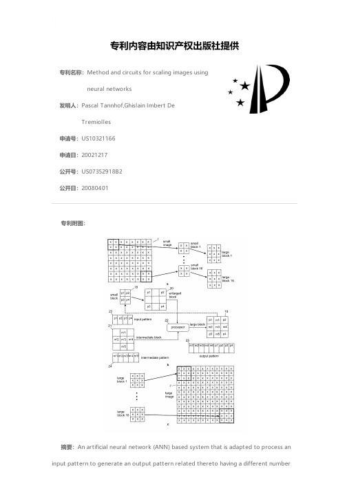
专利名称:Method and circuits for scaling images usingneural networks发明人:Pascal Tannhof,Ghislain Imbert DeTremiolles申请号:US10321166申请日:20021217公开号:US07352918B2公开日:20080401专利内容由知识产权出版社提供专利附图:摘要:An artificial neural network (ANN) based system that is adapted to process an input pattern to generate an output pattern related thereto having a different numberof components than the input pattern. The system () is comprised of an ANN () and a memory (), such as a DRAM memory, that are serially connected. The input pattern () is applied to a processor (), where it can be processed or not (the most general case), before it is applied to the ANN and stored therein as a prototype (if learned). A category is associated with each stored prototype. The processor computes the coefficients that allow the determination of the estimated values of the output pattern, these coefficients are the components of a so-called intermediate pattern (). Assuming the ANN has already learned a number of input patterns, when a new input pattern is presented to the ANN in the recognition phase, the category of the closest prototype is output therefrom and is used as a pointer to the memory. In turn, the memory outputs the corresponding intermediate pattern. The input pattern and the intermediate pattern are applied to the processor to construct the output pattern () using the coefficients. Typically, the input pattern is a block of pixels in the field of scaling images.申请人:Pascal Tannhof,Ghislain Imbert De Tremiolles地址:Fontainebleau FR,Saint Paul FR国籍:FR,FR代理机构:Heslin Rothenberg Farley & Mesiti, P.C.代理人:William H. Steinberg, Esq.,Kevin P. Radigan, Esq.更多信息请下载全文后查看。
机器学习算法在分子结构预测中的应用

机器学习算法在分子结构预测中的应用近年来,随着机器学习领域的不断发展,其在化学领域的应用也越来越广泛。
其中之一的应用就是在分子结构预测中,利用机器学习算法对分子进行预测和模拟,以提高化学领域的研究效率及准确性。
本文将探讨机器学习算法在分子结构预测中的应用,包括现有研究中的案例分析,其中的涉及原理与方法、技术特征、优缺点以及未来发展方向。
一、机器学习算法在分子结构预测中的原理与方法1.1 机器学习算法原理传统的模拟方法,对于计算分子结构的结构、性质、反应等各方面参数往往需要花费大量的精力和计算资源,因此需要发展更加高效、准确和智能化的预测算法。
机器学习算法据此而生,它是对归纳学习和统计学习的综合应用,通过从大量数据中自动提取有价值的特征,并通过训练模型来预测未知数据的方法。
具体而言,机器学习算法需要从大量数据中自动学习分析规律,并且根据新数据更新其模型,以提高预测精度。
1.2 机器学习算法在分子结构预测中的主要方法机器学习算法有许多不同的方法,包括回归、聚类、分类和深度学习等。
在分子结构预测中,回归分析技术、支持向量机和人工神经网络等都有广泛的应用。
(1)回归分析技术:回归分析是一种统计学上的方法,其主要目的是为了确定两个或多个变量之间的关系。
这种方法通常会基于数学公式和数据进行计算,以求出每个参数(自变量)与指定的数据属性之间的关系。
在分子结构预测中,回归分析常被用来拟合一个数学模型,以通过预测的方法预测未知的数据值。
(2)支持向量机:支持向量机(SVM)是一种常见的分类算法,用于建立数据的非线性模型,以便在将来预测数据。
SVM的基本思想是将数据映射到高维空间中,使其能够更好地进行分类。
在分子结构预测中,SVM常用来分类分子,以拟合特定系统中的结构、性质和反应等数据集。
(3)人工神经网络:人工神经网络是一种利用神经元之间互相连接的系统来帮助解决复杂任务的算法。
它借鉴人类大脑的结构与功能,能够通过自适应和归纳学习来提高预测精度。
机器学习在分子设计中的应用

机器学习在分子设计中的应用随着人类对分子结构及其影响力的理解逐渐加深,分子设计已成为人类探索科学与技术的重要途径之一。
在分子设计过程中,人们通常会利用软件进行分子模拟并进行分子设计。
传统的分子设计方法大多需要经验、反复试验和大量时间,效率低下,而机器学习技术则提供了一种更高效的分子设计方法。
机器学习在分子设计中的应用,以其高效、精准和快速的特点受到了广泛的关注。
机器学习是一种通过训练计算机算法并自动实现任务的人工智能技术。
在分子设计领域,机器学习技术可用于生成新的高效药物、材料或催化剂。
机器学习技术大大减少了模拟和实验所需的时间和成本,同时还可以提高设计的成功率。
根据需要进行训练后,机器学习可以自动识别、分类和生成新的分子,从而使多个样本得以快速筛选,并最终得到最合适的设计方案。
机器学习在分子设计中的应用可以分为两种基本类型:有监督学习和无监督学习。
有监督学习是指已经有一些“标准”的样本的情况下,通过计算机的辨认学习,使其对未知的样本进行更好的辨别、分类、回归等等任务。
有监督学习在分子设计中可以用于寻找给定性质的新材料,通过计算机的学习和推理,自动预测其特性,从而实现最优组合的优化。
对于无监督学习,训练数据中存在着相互独立但含有足够多信息的样本数据,其目标是发现数据的固有结构,并分析数据间的潜在相似性和联系,无监督在分子设计中可以用于从大量数据中搜索相似分子候选组合,在最优组合的基础上进行分子生成和设计。
例如,近些年来,基于机器学习的自动驱动分子生成工具已经成为研究分子设计中的关键工具。
这种自动分子生成工具可以基于机器学习对分子进行自主设计,进而自动搜索更多分子。
其准确性和速度比以往的分子设计方法都高得多。
同时,这种工具可以帮助研究人员探索新型化合物,扩大探索范围,也有利于找到隐藏在数据中的新的关联信息。
此外,机器学习算法也可以用于生成和优化分子的三维结构。
该技术包括神经网络、核磁共振计算、蒙特卡罗模拟和多种优化算法等等。
一种改进的混合遗传算法

一种改进的混合遗传算法[提要]为了提高遗传算法的搜索效率,给出了一种改进的遗传算法。
该算法提出了新的交叉操作和仿粒子群变异,扩大了搜索范围。
通过经典函数的测试表明,改进算法与一般自适应遗传算法相比较,在函数最优值、平均收敛代数、收敛概率等方面都取得了令人满意的效果。
关键词:自适应遗传算法;适应度函数;交叉操作;仿粒子群变异中图分类号:TP3 文献标识码:A收录日期:2012年1月12日一、引言遗传算法(GA)由美国Michigan大学的Holland教授于1975年首先提出,后经De Jong、GoldBerg等人改进推广,广泛应用于各类问题。
它是一种模拟自然界生物进化过程与机制的全局概率优化搜索方法。
早期遗传算法在进化过程中易出现早熟收敛和局部收敛性差等问题,为了克服上述问题,人们提出了多种改进算法,本文针对遗传算法的不足,采用实数编码对遗传算法中的交叉和变异操作进行改进,提高了算法全局搜索能力,最后使用改进的算法进行仿真实验,结果表明本算法具有收敛概率高和平均收敛代数少的优点。
二、改进的遗传算法1、改进的交叉操作。
本文遗传算法采用实数编码,改进的交叉操作是先在交叉前产生三个服从均匀分布的随机数a∈[0,1]、b∈[-1,1]、c∈[-1,1],然后假设x1,x2是要交叉的两个父代,个体变量为m维,则x1,x2可以表示为x1=(x11,x12,…,x1m),x2=(x21,x22,…,x2m),其中为位移变量,其中?驻ij=min{(xij-),(-xij)}(i=1,2;j=1,2,…m),最后进行两次操作得:x1’=x1+b•?驻1x2’=x2+c•?驻2 (1)x1’’=ax1’+(1-a)x2’x2’’=ax2’+(1-a)x1’ (2)x1’,x2’,x1’’,x2’’分别为两次操作所产生的子代,从这4个子代中选取适应度大的两个保留到下一代。
通过这种操作可以有效地避免两个数值相近的个体进行“近亲繁殖”(数值相近的个体若只进行(2)式的操作会导致种群多样性快速下降),同时由于b,c的选取,生成的x1’,x2’是两个不相干的个体,彼此之间独立,由(2)式决定的后代还可以使子代遗传父代的某些有用因素,同时由于(1)式的位移调整,使得(2)式生成的后代比一般的算数交叉产生后代的范围扩大,提高算法的搜索范围,避免搜索陷入一个局部区域而出现“早熟”,最后再引入竞争机制在这四个后代中选出两个最好后代个体,这样在保证多样性的同时可以加快收敛的速度。
神经元模式分类器学习的进化计算算法

神经元模式分类器学习的进化计算算法
刘健勤;魏敏洁
【期刊名称】《计算机应用与软件》
【年(卷),期】2000(017)010
【摘要】本文提出了一种用于神经元模式分类器学习的进化计算算法.该算法综合了非确定有限自动机和次群体的动态数据结构,可有效地完成神经网络模式分类器的结构学习,以获得最优的求解结果.该算法的有效性已由计算机仿真实验所证实,可被认为是一种很有发展前途的模式分类系统的机器学习算法.
【总页数】5页(P34-38)
【作者】刘健勤;魏敏洁
【作者单位】中南工业大学自动控制工程系长沙 410083;中南工业大学自动控制工程系长沙 410083
【正文语种】中文
【中图分类】TP31
【相关文献】
1.基于向量机学习算法的多模式分类器的研究及改进 [J], 柳长源;毕晓君;韦琦
2.基于进化计算的贝叶斯网络结构复合学习算法 [J], 刘霄;李海军;尉建华
3.采用进化计算的BP神经网络学习算法研究 [J], 皮亦鸣;李毓生;黄顺吉
4.局部二值模式分类器耦合特征脸的人脸识别算法 [J], 樊颖军
5.一种用于模式分类的多层感知机模型和学习算法 [J], 姜文彬
因版权原因,仅展示原文概要,查看原文内容请购买。
