A signal subspace approach for speech enhancement

合集下载

ESPRIT算法

ESPRIT 算法(Estimating Signal Parameters via Rotational Invariance Techniques)利用子空间旋转方法估计噪声中复正弦信号的频率和幅度, ESPRIT 方法利用了两个时间上互相位移的数据集张成的信号子空间的旋转不变性, 通过广义特征值估计复正弦信号的频率.预备知识: 广义特征值和特征向量设A 和B 是两个n n ⨯的矩阵, 具有形式B A λ-的所有矩阵组称为矩阵束(Matrix pencil)(也表示成(A,B)), λ是任意复数, 矩阵束的广义特征值集合),(B A λ定义为:{}0)det(),(=-∈=zB A C z B A λ更一般的定义: 使(A-zB)降秩的z 值集合若),(B A λλ∈, 如果有一矢量0x x ≠,, 满足x x B A λ= 则称x 是矩阵束B A λ-的广义特征矢量.ESPRIT 算法:信号模型为)()(1k n e s k x d i jk i i +=∑=ω(1)这里, ),(ππω-∈i 是归一化频率, i s 是第i 个复正弦的复幅度值. n(k)是零均值平稳的复高斯白噪声, 目的是通过观察数据估计各复正弦的频率和幅度.为了利用复正弦信号的相关矩阵的性质, 定义x(n)的时间位移信号y(n).y(n)=x(n+1)并定义如下m 维矢量(这里要求m>d )[][][][]T T T T m k x k x m k y k y k m k n k n k m k x k x k )(,),1()1(,),()()1(,),()()1(,),()(++=-+=-+=-+= y n x (2) 由信号模型(1), 我们可以得到如下矩阵表示.)1()()()(++Φ=+=k A k k A k n s y n s x 这里, Td s s ],[1 =s 是复正弦的幅度矢量, Φ是d ⨯d 矩阵, 它反映了x 和y 之间的时移关系,又称为旋转算子.它可以写成],[1d j j e e diag ωω =ΦA 是m ⨯d V andermonde 矩阵, 它的列矢量{}d i i ,1);(=ωa 定义为:[]Tm j j i i i e e ωωω)1(,,1)(-= a . 通过这些表示, x 的自相关矩阵可以写成:[]I ASA k k E R H H xx 2)()(σ+==x x 这里, S 是d ⨯d 对角矩阵, 每个元素对应于一个复正弦的功率, 即 []221,d s s diag S =但实际上ESPRIT 算法并不要求S 一定是对角矩阵, 它只要是非奇异的. 类似地, x 和y 的互相关矩阵为:[]Z A AS k k E R H H H xy 2)()(σ+Φ==y x注意, [])1()(2+=k k E Z H n n σ, Z 是m ⨯m 矩阵, 它的次对角元素为1, 其它元素为零, 即⎥⎥⎥⎥⎥⎥⎦⎤⎢⎢⎢⎢⎢⎢⎣⎡=010********* Z 两个相关矩阵分别可以写成:[][]**)()(i j j i ij xx r r j x i x E R --=== 即⎥⎥⎥⎥⎥⎦⎤⎢⎢⎢⎢⎢⎣⎡=----021*201*1*10r r r r r r r r r R m m m m xx 互相关[][]1*)1()(--=+=j i ij xy r j x i x E R ⎥⎥⎥⎥⎥⎦⎤⎢⎢⎢⎢⎢⎣⎡=---*132*1*10**2*1r r r r r r r r r R m m m m xy 根据这些模型关系和一组相关值, 估计复正弦参数.估计算法的基础是如下定理, 这个定理的证明主要依赖于x 和y 矢量构成的信号子空间的旋转不变性.定理:定义矩阵束{}xy xx C C ,, 这里I R C xx xx min λ-=和Z R C xy xy min λ-=, min λ是xx R 的最小特征值. 定义Γ是矩阵束的广义特征值矩阵, 如果S 是非奇异的, 则Φ和Γ具备如下关系:⎥⎦⎤⎢⎣⎡Φ=Γ000 该式中Φ的元素可能是重排列的.#证明:A 是满秩矩阵, S 是非奇异的, 故H ASA 的秩是d , 因此xx R 具有m-d 阶特征值2σ, 它是最小特征值, 因此,H H xy xy xy Hxx xx xx AAS Z R Z R C ASA I R I R C Φ=-=-==-=-=2min 2min σλσλ 现在考虑矩阵束H H xy xx A I AS C C )(Φ-=-γγ容易检查, H ASA 和H H A AS Φ的列空间是一致的, 对一般的γ取值, H H xy xx A I AS C C )(Φ-=-γγ的秩为d, 只有当i j e ωγ=, )(H I Φ-γ的第i 行为零, H H xy xx A I AS C C )(Φ-=-γγ的秩降为d-1, 按定义, i j e ωγ=是矩阵束的一个广义特征值, 这样的特征值有d 个, 其余m-d 个广义特征值为零.#由如上定理, 得到ESPRIT 算法如下:1) 由观测数据得到{}m r r r ,,10的估计值.2) 由{}m r r r ,,10构造自相关和互相关矩阵xy xx R R ,3) 对xx R 作特征分解, 对于m>d, 最小特征值是2σ4) 计算(xy xx C C ,), (H ASA ,H H A AS Φ)5) 计算矩阵束(xy xx C C ,)= (H ASA ,H H A AS Φ)的广义特征值, 在单位圆上的对应复正弦的频率, 其它为0.6) 设广义特征值i γ的特征矢量记为:i v , 由()0=Φ-i H H i A I AS v γ可以导出:)(2i H i i xx H i i C s ωa v v v =实际中,由于只有估计的自相关序列值, 因此, 如上理论只是被近似满足, 在这些限制条件下, 有一些改进方法已经用于ESPRIT估计算法中.参考文献:1.R. Roy, A. Paulraj, and T. Kailath, “ESPRIT—A Subspace rotation approach to estimation ofparameters of cissoids in noise”, IEEE Trans. On Acoustics, Speech, and Signal Processing, V ol. 34, No.5, Oct. 19862.R. Roy, and T. Kailath, “ESPRIT—Estimation of Signal Parameters Via RotationalInvariance Techniques”, IEEE Trans. On Acoustics, Speech, and Signal Processing, V ol.37, No.7, July 1989.。

Subspace Pursuit for Compressive Sensing Signal

a r X i v :0803.0811v 3 [c s .N A ] 8 J a n 2009Subspace Pursuit for Compressive Sensing SignalReconstructionWei Dai and Olgica MilenkovicDepartment of Electrical and Computer EngineeringUniversity of Illinois at Urbana-ChampaignAbstract —We propose a new method for reconstruction of sparse signals with and without noisy perturbations,termed the subspace pursuit algorithm.The algorithm has two important characteristics:low computational complexity,comparable to that of orthogonal matching pursuit techniques when applied to very sparse signals,and reconstruction accuracy of the same order as that of LP optimization methods.The presented analysis shows that in the noiseless setting,the proposed algorithm can exactly reconstruct arbitrary sparse signals provided that the sensing matrix satisﬁes the restricted isometry property with a constant parameter.In the noisy setting and in the case that the signal is not exactly sparse,it can be shown that the mean squared error of the reconstruction is upper bounded by constant multiples of the measurement and signal perturbation energies.Index Terms —Compressive sensing,orthogonal matching pur-suit,reconstruction algorithms,restricted isometry property,sparse signal reconstruction.I.I NTRODUCTIONCompressive sensing (CS)is a sampling method closely connected to transform coding which has been widely used in modern communication systems involving large scale data samples.A transform code converts input signals,embedded in a high dimensional space,into signals that lie in a space of signiﬁcantly smaller dimensions.Examples of transform coders include the well known wavelet transforms and the ubiquitous Fourier transform.Compressive sensing techniques perform transform cod-ing successfully whenever applied to so-called compressible and/or K -sparse signals,i.e.,signals that can be represented by K ≪N signiﬁcant coefﬁcients over an N -dimensional basis.Encoding of a K -sparse,discrete-time signal x of dimension N is accomplished by computing a measurement vector y that consists of m ≪N linear projections of the vector x .This can be compactly described viay =Φx .Here,Φrepresents an m ×N matrix,usually over the ﬁeld of real numbers.Within this framework,the projection basis is assumed to be incoherent with the basis in which the signal has a sparse representation [1].Although the reconstruction of the signal x ∈R N from the possibly noisy random projections is an ill-posed problem,theThis work is supported by NSF Grants CCF 0644427,0729216and the DARPA Young Faculty Award of the second author.Wei Dai and Olgica Milenkovic are with the Department of Electrical and Computer Engineering,University of Illinois at Urbana-Champaign,Urbana,IL 61801-2918USA (e-mail:weidai07@;milenkov@).strong prior knowledge of signal sparsity allows for recovering x using m ≪N projections only.One of the outstanding results in CS theory is that the signal x can be reconstructed using optimization strategies aimed at ﬁnding the sparsest signal that matches with the m projections.In other words,the reconstruction problem can be cast as an l 0minimization problem [2].It can be shown that to reconstruct a K -sparse signal x ,l 0minimization requires only m =2K random pro-jections when the signal and the measurements are noise-free.Unfortunately,the l 0optimization problem is NP-hard.This issue has led to a large body of work in CS theory and practice centered around the design of measurement and reconstruction algorithms with tractable reconstruction complexity.The work by Donoho and Candès et.al.[1],[3],[4],[5]demonstrated that CS reconstruction is,indeed,a polynomial time problem –albeit under the constraint that more than 2K measurements are used.The key observation behind these ﬁndings is that it is not necessary to resort to l 0optimization to recover x from the under-determined inverse problem;a much easier l 1optimization,based on Linear Programming (LP)techniques,yields an equivalent solution,as long as the sampling matrix Φsatisﬁes the so called restricted isometry property (RIP)with a constant parameter.While LP techniques play an important role in designing computationally tractable CS decoders,their complexity is still highly impractical for many applications.In such cases,the need for faster decoding algorithms -preferably operating in linear time -is of critical importance,even if one has to increase the number of measurements.Several classes of low-complexity reconstruction techniques were recently put forward as alternatives to linear programming (LP)based recovery,which include group testing methods [6],and al-gorithms based on belief propagation [7].Recently,a family of iterative greedy algorithms received signiﬁcant attention due to their low complexity and simple geometric interpretation.They include the Orthogonal Match-ing Pursuit (OMP),the Regularized OMP (ROMP)and the Stagewise OMP (StOMP)algorithms.The basic idea behind these methods is to ﬁnd the support of the unknown signal sequentially.At each iteration of the algorithms,one or several coordinates of the vector x are selected for testing based on the correlation values between the columns of Φand the regularized measurement vector.If deemed sufﬁciently reliable,the candidate column indices are subsequently added to the current estimate of the support set of x .The pursuit algorithms iterate this procedure until all the coordinates inthe correct support set are included in the estimated support set.The computational complexity of OMP strategies depends on the number of iterations needed for exact reconstruction:standard OMP always runs through K iterations,and there-fore its reconstruction complexity is roughly O(KmN)(see Section IV-C for details).This complexity is signiﬁcantly smaller than that of LP methods,especially when the signal sparsity level K is small.However,the pursuit algorithms do not have provable reconstruction quality at the level of LP methods.For OMP techniques to operate successfully,one requires that the correlation between all pairs of columns ofΦis at most1/2K[8],which by the Gershgorin Circle Theorem[9]represents a more restrictive constraint than the RIP.The ROMP algorithm[10]can reconstruct all K-sparse signals provided that the RIP holds with parameter δ2K≤0.06/√log K.The main contribution of this paper is a new algorithm, termed the subspace pursuit(SP)algorithm.It has provable reconstruction capability comparable to that of LP methods, and exhibits the low reconstruction complexity of matching pursuit techniques for very sparse signals.The algorithm can operate both in the noiseless and noisy regime,allowing for exact and approximate signal recovery,respectively.For any sampling matrixΦsatisfying the RIP with a constant parameter independent of K,the SP algorithm can recover arbitrary K-sparse signals exactly from its noiseless mea-surements.When the measurements are inaccurate and/or the signal is not exactly sparse,the reconstruction distortion is upper bounded by a constant multiple of the measurementand/or signal perturbation energy.For very sparse signals√with K≤const·3 the main result of the paper pertaining to the noiseless setting:a formal proof for the guaranteed reconstruction performanceand the reconstruction complexity of the SP algorithm.Sec-tion V contains the main result of the paper pertaining to thenoisy setting.Concluding remarks are given in Section VI,while proofs of most of the theorems are presented in theAppendix of the paper.II.P RELIMINARIESpressive Sensing and the Restricted Isometry PropertyLet supp(x)denote the set of indices of the non-zerocoordinates of an arbitrary vector x=(x1,...,x N),and let|supp(x)|= · 0denote the support size of x,or equivalently,its l0norm1.Assume next that x∈R N is an unknown signalwith|supp(x)|≤K,and let y∈R m be an observation of xvia M linear measurements,i.e.,y=Φx,whereΦ∈R m×N is henceforth referred to as the samplingmatrix.We are concerned with the problem of low-complexityrecovery of the unknown signal x from the measurement y.A natural formulation of the recovery problem is within an l0norm minimization framework,which seeks a solution to theproblemmin xsubject to y=Φx.Unfortunately,the above l0minimization problem is NP-hard,and hence cannot be used for practical applications[3],[4].One way to avoid using this computationally intractable for-mulation is to consider a l1-regularized optimization problem,min x1subject to y=Φx,wherex 1=N i=1|x i|denotes the l1norm of the vector x.The main advantage of the l1minimization approach is thatit is a convex optimization problem that can be solved efﬁ-ciently by linear programming(LP)techniques.This methodis therefore frequently referred to as l1-LP reconstruction[3],[13],and its reconstruction complexity equals O m2N3/2 when interior point methods are employed[14].See[15],[16],[17]for other methods to further reduce the complexity of l1-LP.The reconstruction accuracy of the l1-LP method is de-scribed in terms of the restricted isometry property(RIP),formally deﬁned below.Deﬁnition1(Truncation):LetΦ∈R m×N,x∈R N and I⊂{1,···,N}.The matrixΦI consists of the columns of Φwith indices i∈I,and x I is composed of the entries of x indexed by i∈I.The space spanned by the columns ofΦI is denoted by span(ΦI).Deﬁnition2(RIP):A matrixΦ∈R m×N is said to satisfythe Restricted Isometry Property(RIP)with parameters(K,δ) 1We interchangeably use both notations in the paper.for K≤m,0≤δ≤1,if for all index sets I⊂{1,···,N} such that|I|≤K and for all q∈R|I|,one has(1−δ) q 22≤ ΦI q 22≤(1+δ) q 22.We deﬁneδK,the RIP constant,as the inﬁmum of all parametersδfor which the RIP holds,i.e.δK:=inf δ:(1−δ) q 22≤ ΦI q 22≤(1+δ) q 22,∀|I|≤K,∀q∈R|I| .Remark1(RIP and eigenvalues):If a sampling matrix Φ∈R m×N satisﬁes the RIP with parameters(K,δK),then for all I⊂{1,···,N}such that|I|≤K,it holds that 1−δK≤λmin(Φ∗IΦI)≤λmax(Φ∗IΦI)≤1+δK, whereλmin(Φ∗IΦI)andλmax(Φ∗IΦI)denote the minimal and maximal eigenvalues ofΦ∗IΦI,respectively.Remark2(Matrices satisfying the RIP):Most known fam-ilies of matrices satisfying the RIP property with optimal or near-optimal performance guarantees are random.Examples include:1)Random matrices with i.i.d.entries that follow eitherthe Gaussian distribution,Bernoulli distribution with zero mean and variance1/n,or any other distribution that satisﬁes certain tail decay laws.It was shown in[13]that the RIP for a randomly chosen matrix fromsuch ensembles holds with overwhelming probability wheneverK≤Cm(log N)6,where C depends only on the RIP constant.There exists an intimate connection between the LP recon-struction accuracy and the RIP property,ﬁrst described by Candés and Tao in[3].If the sampling matrixΦsatisﬁes the RIP with constantsδK,δ2K,andδ3K,such thatδK+δ2K+δ3K<1,(1) then the l1-LP algorithm will reconstruct all K-sparse signals exactly.This sufﬁcient condition(1)can be improved toδ2K<√4Lemma1(Consequences of the RIP):1)(Monotonicity ofδK)For any two integers K≤K′,δK≤δK′.2)(Near-orthogonality of columns)Let I,J⊂{1,···,N} be two disjoint sets,I J=φ.Suppose thatδ|I|+|J|<1.For arbitrary vectors a∈R|I|and b∈R|J|,| ΦI a,ΦJ b |≤δ|I|+|J| a 2 b 2,andΦ∗IΦJ b 2≤δ|I|+|J| b 2.The lemma implies thatδK≤δ2K≤δ3K,which conse-quently simpliﬁes(1)toδ3K<1/3.Both(1)and(2)represent sufﬁcient conditions for exact reconstruction.In order to describe the main steps of the SP algorithm,we introduce next the notion of the projection of a vector and its residue.Deﬁnition3(Projection and Residue):Let y∈R m and ΦI∈R m×|I|.Suppose thatΦ∗IΦI is invertible.The projection of y onto span(ΦI)is deﬁned asy p=proj(y,ΦI):=ΦIΦ†I y,whereΦ†I:=(Φ∗IΦI)−1Φ∗Idenotes the pseudo-inverse of the matrixΦI,and∗stands for matrix transposition.The residue vector of the projection equalsy r=resid(y,ΦI):=y−y p.Weﬁnd the following properties of projections and residues of vectors useful for our subsequent derivations.Lemma2(Projection and Residue):1)(Orthogonality of the residue)For an arbitrary vectory∈R m,and a sampling matrixΦI∈R m×K of full column rank,let y r=resid(y,ΦI).ThenΦ∗I y r=0.2)(Approximation of the projection residue)Consider amatrixΦ∈R m×N.Let I,J⊂{1,···N}be two disjoint sets,I J=φ,and suppose thatδ|I|+|J|<1.Furthermore,let y∈span(ΦI),y p=proj(y,ΦJ)and y r=resid(y,ΦJ).Theny p 2≤δ|I|+|J|1−δmax(|I|,|J|) y 2≤ y r 2≤ y 2.(4) The proof of Lemma2can be found in Appendix B.III.T HE SP A LGORITHMThe main steps of the SP algorithm are summarized below.2 Input:K,Φ,yInitialization:1)T0={K indices corresponding to the largest magni-tude entries in the vectorΦ∗y}.2)y0r=resid y,ΦˆT0 .Iteration:At theℓth iteration,go through the following steps 1)˜Tℓ=Tℓ−1 {K indices corresponding to the largestmagnitude entries in the vectorΦ∗yℓ−1r .2)Set x p=Φ†˜Tℓy.3)Tℓ={K indices corresponding to the largest elementsof x p}.4)yℓr=resid(y,ΦTℓ).5)If yℓr 2> yℓ−1r 2,let Tℓ=Tℓ−1and quit theiteration.Output:1)The estimated signalˆx,satisfyingˆx{1,···,N}−Tℓ=0andˆx Tℓ=Φ†Tℓy.5(a)Iterations in OMP,Stagewise OMP,and Regularized OMP:in each iteration,one decides on a reliable set of candidate indices to be added into the list T ℓ−1;once a candidate is added,it remains in the list until the algorithmterminates.(b)Iterations in the proposed Subspace Pursuit Algorithm:a list of K can-didates,which is allowed to be updated during the iterations,is maintained.Figure 1:Description of reconstruction algorithms for K -sparse signals:though both approaches look similar,the basic ideas behind them are quite different.exact reconstruction for the Gaussian random matrix ensemble.The steps of the testing strategy are listed below.1)For given values of the parameters m and N ,choose a signal sparsity level K such that K ≤m/2;2)Randomly generate a m ×N sampling matrix Φfrom the standard i.i.d.Gaussian ensemble;3)Select a support set T of size |T |=K uniformly at random,and generate the sparse signal vector x by either one of the following two methods:a)Draw the elements of the vector x restricted to T from the standard Gaussian distribution;we refer to this type of signal as a Gaussian signal.Or,b)set all entries of x supported on T to ones;we refer to this type of signal as a zero-one signal.Note that zero-one sparse signals are of special interest for the comparative study,since they represent a partic-ularly challenging case for OMP-type of reconstruction strategies.4)Compute the measurement y =Φx ,apply a recon-struction algorithm to obtain ˆx,the estimate of x ,and compare ˆxto x ;5)Repeat the process 500times for each K ,and then simulate the same algorithm for different values of m and N .The improved reconstruction capability of the SP method,compared with that of the OMP andROMP algorithms,is illustrated by two examples shown in Fig.2.Here,the signals are drawn both according to the Gaussian and zero-one model,and the benchmark performance of the LP reconstruction(a)Simulations for Gaussian sparse signals:OMP and ROMP start to fail when K ≥19and when K ≥22respectively,ℓ1-LP begins to fail when K ≥35,and the SP algorithm fails only when K ≥45.(b)Simulations for zero-one sparse signals:both OMP and ROMP starts to fail when K ≥10,ℓ1-LP begins to fail when K ≥35,and the SP algorithm fails when K ≥29.Figure 2:Simulations of the exact recovery rate:compared with OMPs,the SP algorithm has signiﬁcantly larger critical sparsity.technique is plotted as well.Figure 2depicts the empirical frequency of exact reconstruc-tion.The numerical values on the x -axis denote the sparsity level K ,while the numerical values on the y -axis represent the fraction of exactly recovered test signals.Of particular interest is the sparsity level at which the recovery rate drops below 100%-i.e.the critical sparsity -which,when exceeded,leads to errors in the reconstruction algorithm applied to some of the signals from the given class.The simulation results reveal that the critical sparsity of the SP algorithm by far exceeds that of the OMP and ROMP techniques,for both Gaussian and zero-one inputs.The re-construction capability of the SP algorithm is comparable to that of the LP based approach:the SP algorithm has a slightly higher critical sparsity for Gaussian signals,but also a slightly6 lower critical sparsity for zero-one signals.However,the SPalgorithms signiﬁcantly outperforms the LP method whenit comes to reconstruction complexity.As we analyticallydemonstrate in the exposition to follow,the reconstructioncomplexity of the SP algorithm for both Gaussian and zero-onesparse signals is O(mN log K),whenever K≤O √1−2δ3K yℓ−1r 2< yℓ−1r 2,(7)where2δ3K(1+δ3K)c K=x T−Tℓ−1 2.(1−δ3K)2The proof of the theorem is postponed to Appendix D.Theorem4:The following inequality is validx T−Tℓ 2≤1+δ3K7 Furthermore,according to Lemmas1and2,one hasyℓr 2= resid(y,ΦTℓ) 2= resid(ΦT−Tℓx T−Tℓ,ΦTℓ)+resid(ΦTℓx Tℓ,ΦTℓ)2D3= resid(ΦT−Tℓx T−Tℓ,ΦTℓ)+02(4)≤ ΦT−Tℓx T−Tℓ 2(6)≤1−δK ΦT−Tℓ−1x T−Tℓ−1 2≥1−2δ2K1−δK x T−Tℓ−1 2≥1−2δ2K1−δKx T−Tℓ−1 2.(10) Upon combining(9)and(10),one obtains the following upper boundyℓr 2≤ 1−2δ2K c K yℓ−1r 2L1≤11−2δ3K<1,which completes the proof of Theorem2.A.Why Does Correlation Maximization Work for the SP Algorithm?Both in the initialization step and during each iteration of the SP algorithm,we select K indices that maximize the correlations between the column vectors and the residual measurement.Henceforth,this step is referred to as correlation maximization(CM).Consider the ideal case where all columns ofΦare orthogonal3.In this scenario,the signal coefﬁcients can be easily recovered by calculating the correlations v i,y -i.e.,all indices with non-zero magnitude are in the correct support of the sensed vector.Now assume that the sampling matrixΦsatisﬁes the RIP.Recall that the RIP(see Lemma 1)implies that the columns are locally near-orthogonal.Con-sequently,for any j not in the correct support,the magnitude of the correlation v j,y is expected to be small,and more precisely,upper bounded byδK+1 x 2.This seems to provide a very simple intuition why correlation maximization allows for exact reconstruction.However,this intuition is not easy 3Of course,in this case no compression is possible.to analytically justify due to the following fact.Although it is clear that for all indices j/∈T,the values of| v j,y |areupper bounded byδK+1 x ,it may also happen that for all i∈T,the values of| v i,y |are small as well.Dealing withmaximum correlations in this scenario cannot be immediately proved to be a good reconstruction strategy.The following example illustrates this point.Example1:Without loss of generality,let T={1,···,K}.Let the vectors v i(i∈T)be orthonormal, and let the remaining columns v j,j/∈T,ofΦbe constructed randomly,using i.i.d.Gaussian samples.Consider the following normalized zero-one sparse signaly=1K i∈T v i.Then,for K sufﬁciently large,| v i,y |=1K≪1,for all1≤i≤K.It is straightforward to envision the existence of an index j/∈T,such that| v j,y |≈δK+1>1K.The latter inequality is critical,because achieving very small values for the RIP constant is a challenging task.This example represents a particularly challenging case for the OMP algorithm.Therefore,one of the major constraints imposed on the OMP algorithm is the requirement that maxi∈T| v i,y |=1K>maxj/∈T|v j,y |≈δK+1.To meet this requirement,δK+1has to be less than1/√8and at least one correct element of the support of x isinT0.This phenomenon is quantitatively described in Theorem5. Theorem5:After the initialization step,one hasx T0T T 2≥1−δK−2δ2K8δ2K−8δ22Kx 2=min1≤i≤K|x i|K i=1x2i.(12)Let n it denote the number of iterations of the SP algorithm needed for exact reconstruction of x.Then the following theorem upper bounds n it in terms of c K andρmin.It can be viewed as a bound on the complexity/performance trade-off for the SP algorithm.Theorem6:The number of iterations of the SP algorithm is upper bounded byn it≤min −logρmin−log c K .This result is a combination of Theorems7and(12),4 described below.4The upper bound in Theorem7is also obtained in[12]while the one in Theorem8is not.9 Theorem7:One hasn it≤−logρmin−log c K.The proof of Theorem7is intuitively clear and presentedbelow,while the proof of Theorem8is more technical andpostponed to Appendix F.Proof of Theorem7:The theorem is proved by contra-diction.Consider Tℓ,the estimate of T,withl= −logρmini∈T−Tℓx2i≥min i∈T|x i|(12)=ρmin x 2.However,according to Theorem2,x T−Tℓ 2≤(c K)ℓ x 2<ρmin x 2,where the last inequality follows from our choice ofℓsuchthat(c K)ℓ<ρmin.This contradicts the assumption T Tℓand therefore proves Theorem7.2.Noting thatρmin 2−10,Theorem6impliesthatn it≤11.Indeed,if we take a close look at the steps of the SP algorithm, we can verify thatn it≤1.After the initialization step,by Theorem5,it can be shown thatx T−T0 2≤ 1+δ2K x 2<0.95 x 2.As a result,the estimate T0must contain the index one and x T−T0 2≤1.After theﬁrst iteration,sincex T−T1 2≤c K x T−T0 <0.95<min i∈T|x i|,we have T⊂T1.This example suggests that the upper bound(7)can be tightened when the signal components decay fast.Based on the idea behind this example,another upper bound on n it is described in Theorem8and proved in Appendix F.It is clear that the number of iterations required for exact re-construction depends on the values of the entries of the sparse signal.We therefore focus our attention on the following three particular classes of sparse signals.1)Zero-one sparse signals.As explained before,zero-onesignals represent the most challenging reconstruction category for OMP algorithms.However,this class of signals has the best upper bound on the convergence rate of the SP algorithm.Elementary calculations reveal thatρmin=1/√2log(1/c K).2)Sparse signals with power-law decaying entries(alsoknown as compressible sparse signals).Signals in this category are deﬁned via the following constraint|x i|≤c x·i−p,for some constants c x>0and p>pressible sparse signals have been widely considered in the CS literature,since most practical and naturally occurring signals belong to this class[13].It follows from Theo-rem7that in this casen it≤p log Klog(1/c K)(1+o(1))if0<p≤1.51.5K10Figure5:Convergence of the subspace pursuit algorithm fordifferent signals.In each iteration,CM requires mN computations in general.For some measurement matrices with special structures,for ex-ample,sparse matrices,the computational cost can be reducedsigniﬁcantly.The cost of computing the projections is of theorder of O K2m ,if one uses the Modiﬁed Gram-Schmidt (MGS)algorithm[20,pg.61].This cost can be reducedfurther by“reusing”the computational results of past iterations within future iterations.This is possible because most practical sparse signals are compressible,and the signal support set estimates in different iterations usually intersect in a large number of indices.Though there are many ways to reduce the complexity of both the CM and projection computation steps,we only focus on the most general framework of the SP algorithm,and assume that the complexity of each iteration equals O mN+mK2 .As a result,the total complexity of the SP algorithm is given by O m N+K2 log K for compressible sparse signals,and it is upper bounded by O m N+K2 K for arbitrary sparse signals.When the signal is very sparse,in particular,when K2≤O(N),the total complexity of SP reconstruction is upper bounded by O(mNK)for arbitrary sparse signals and by O(mN log K) for compressible sparse signals(we once again point out that most practical sparse signals belong to this signal category [13]).The complexity of the SP algorithm is comparable to OMP-type algorithms for very sparse signals where K2≤O(N). For the standard OMP algorithm,exact reconstruction always requires K iterations.In each iteration,the CM operation costs O(mN)computations and the complexity of the projection is marginal compared with the CM.The corresponding total complexity is therefore always O(mNK).For the ROMP and StOMP algorithms,the challenging signals in terms of convergence rate are also the sparse signals with exponentially decaying entries.When the p in(13)is sufﬁciently large,it can be shown that both ROMP and StOMP also need O(K)iter-ations for reconstruction.Note that CM operation is required in both algorithms.The total computational complexity is then O(mNK).The case that requires special attention during analysisis K2>O(N).Again,if compressible sparse signals are considered,the complexity of projections can be signiﬁcantly reduced if one reuses the results from previous iterations at thecurrent iteration.If exponentially decaying sparse signals areconsidered,one may want to only recover the energetically most signiﬁcant part of the signal and treat the residual ofthe signal as noise—reduce the effective signal sparsity to K′≪K.In both cases,the complexity depends on the speciﬁc implementation of the CM and projection operationsand is beyond the scope of analysis of this paper.One advantage of the SP algorithm is that the number of iterations required for recovery is signiﬁcantly smaller than that of the standard OMP algorithm for compressible sparse signals.To the best of the authors’knowledge,there are no known results on the number of iterations of the ROMP and StOMP algorithms needed for recovery of compressible sparse signals.V.R ECOVERY OF A PPROXIMATELY S PARSE S IGNALSFROM I NACCURATE M EASUREMENTSWeﬁrst consider a sampling scenario in which the signal x is K-sparse,but the measurement vector y is subjected to an additive noise component,e.The following theorem gives a sufﬁcient condition for convergence of the SP algorithm in terms of the RIP constantδ3K,as well as an upper bounds on the recovery distortion that depends on the energy(l2-norm) of the error vector e.Theorem9(Stability under measurement perturbations): Let x∈R N be such that|supp(x)|≤K,and let its corresponding measurement be y=Φx+e,where e denotes the noise vector.Suppose that the sampling matrix satisﬁes the RIP with parameterδ3K<0.083.(14) Then the reconstruction distortion of the SP algorithm satisﬁesx−ˆx 2≤c′K e 2,wherec′K=1+δ3K+δ23K11Thenx −ˆx 2≤c ′2Ke 2+Kx −x K 1.The proof of this corollary is given in SectionV-B.Asopposed to the standard case where the input sparsity level of the SP algorithm equals the signal sparsity level K ,one needs to set the input sparsity level of the SP algorithm to 2K in order to obtain the claim stated in the above corollary.Theorem 9and Corollary 1provide analytical upper bounds on the reconstruction distortion of the noisy version of the SP algorithm.In addition to these theoretical bounds,we performed numerical simulations to empirically estimate the reconstruction distortion.In the simulations,we ﬁrst select the dimension N of the signal x ,and the number of measurements m .We then choose a sparsity level K such that K ≤m/2.Once the parameters are chosen,an m ×N sampling matrix with standard i.i.d.Gaussian entries is generated.For a given K ,the support set T of size |T |=K is selected uniformly at random.A zero-one sparse signal is constructed as in the previous section.Finally,either signal or a measurement perturbations are added as follows:1)Signal perturbations :the signal entries in T are kept un-changed but the signal entries outside of T are perturbed by i.i.d.Gaussian N 0,σ2s samples.2)Measurement perturbation s:the perturbation vector e is generated using a Gaussian distribution with zero meanand covariance matrix σ2e I m ,where I m denotes the m ×m identity matrix.We ran the SP reconstruction process on y ,500times foreach K ,σ2s and σ2e .The reconstruction distortion x −ˆx2is obtained via averaging over all these instances,and the results are plotted in Fig.6.Consistent with the ﬁndings of Theorem 9and Corollary 1,we observe that the recovery dis-tortion increases linearly with the l 2-norm of the measurement error.Even more encouraging is the fact that the empirical reconstruction distortion is typically much smaller than the corresponding upper bounds.This is likely due to the fact that,in order to simplify the expressions involved,many constants and parameters used in the proof were upper bounded.A.Recovery Distortion under Measurement Perturbations The ﬁrst step towards proving Theorem 9is to upper boundthe reconstruction error for a given estimated support set ˆT,as succinctly described in the lemma to follow.Lemma 3:Let x ∈R N be a K -sparse vector, x 0≤K ,and let y =Φx +e be a measurement for which Φ∈R m ×Nsatisﬁes the RIP with parameter δK .For an arbitrary ˆT ⊂{1,···,N }such that ˆT≤K ,deﬁne ˆxas ˆx ˆT =Φ†ˆT y ,andˆx {1,···,N }−ˆT =0.Thenx −ˆx2≤11−δ3Ke 2.Figure 6:Reconstruction distortion under signal or measure-ment perturbations:both perturbation level and reconstruction distortion are described via the l 2norm.The proof of the lemma is given in Appendix G.Next,we need to upper bound the norm x T −T ℓ 2in the ℓthiteration of the SP algorithm.To achieve this task,we describe in the theorem to follow how x T −T ℓ 2depends on the RIP constant and the noise energy e 2.Theorem 10:It holds that x T −˜T ℓ 2≤2δ3K 1−δ3Ke 2,(15)x T −T ℓ 2≤1+δ3K1−δ3Ke 2,(16)and therefore, x T −T ℓ 2≤2δ3K (1+δ3K )(1−δ3K )2e 2.(17)Furthermore,suppose thate 2≤δ3K x T −T ℓ−1 2.(18)Then one has y ℓr 2< y ℓ−1r 2wheneverδ3K <0.083.Proof:The upper bounds in Inequalities (15)and (16)areproved in Appendix H and I,respectively.The inequality (17)is obtained by substituting (15)into (16)as shown below:x T −T ℓ 2≤2δ3K (1+δ3K )(1−δ3K )2e 2≤2δ3K (1+δ3K )(1−δ3K )2e 2.。

现代语言学前五章课后习题答案

Chapter 1 Introduction1.Explain the following definition of linguistics: Linguistics is the scientific study oflanguage. 请解释以下语言学的定义:语言学是对语言的科学研究。

Linguistics investigates not any particular languagebut languages in general.Linguistic study is scientific because it is baxxxxsed on the systematic investigation of authentic language data.No serious linguistic conclusion is reached until after the linguist has done the following three things: observing the way language is actually usedformulating some hypothesesand testing these hypotheses against linguistic facts to prove their validity.语言学研究的不是任何特定的语言，而是一般的语言。

语言研究是科学的，因为它是建立在对真实语言数据的系统研究的基础上的。

只有在语言学家做了以下三件事之后，才能得出严肃的语言学结论:观察语言的实际使用方式，提出一些假设，并用语言事实检验这些假设的正确性。

1.What are the major branches of linguistics? What does each of them study?语言学的主要分支是什么?他们每个人都研究什么?Phonetics-How speech sounds are produced and classified语音学——语音是如何产生和分类的Phonology-How sounds form systems and function to convey meaning音系学——声音如何形成系统和功能来传达意义Morphology-How morphemes are combined to form words形态学——词素如何组合成单词Sytax-How morphemes and words are combined to form sentences句法学-词素和单词如何组合成句子Semantics-The study of meaning ( in abstraction)语义学——意义的研究(抽象)Pragmatics-The study of meaning in context of use语用学——在使用语境中对意义的研究Sociolinguistics-The study of language with reference to society社会语言学——研究与社会有关的语言Psycholinguistics-The study of language with reference to the workings of the mind心理语言学:研究与大脑活动有关的语言Applied Linguistics-The application of linguistic principles and theories to language teaching and learning应用语言学——语言学原理和理论在语言教学中的应用1.What makes modern linguistics different from traditional grammar?现代语言学与传统语法有何不同?Modern linguistics is descxxxxriptive;its investigations are baxxxxsed on authenticand mainly spoken language data.现代语言学是描述性的，它的研究是基于真实的，主要是口语数据。

信号子空间语音增强和它的应用对噪声语音识别研究文章

研究文章回顾信号子空间语音增强和它的应用对噪声语音识别克里斯赫墨思,帕特里克，和雨果·范·哈默电机工程学系，天主教鲁汶大学，比利时鲁汶赫维2005年10月收到24份修订于2006年3月2006年4月30日由三颗针科斯塔斯卡推荐本文的目的有三个方面：（1）提供了广泛的审查，（2）派生的信号子空间语音增强这些技术的性能的上限，（3）提出了全面的研究子空间的潜力过滤，以增加对固定加性噪声失真自动语音识别器的特性。

子空间滤波方法是基于嘈杂的讲话观测空间的正交分解成信号子空间和噪声子空间。

这种分解可以用于语音模型的低秩的假设下，对是否有可用的估计的噪声相关矩阵。

我们提出了一个广泛的概述可用的估计，并从中获得了理论估计实验评估的上限的性能，可以实现由任何基于子空间的方法。

与噪声数据的自动语音识别（ASR）的实验表明，基于子空间的语音增强显着提高这些系统的特性添加剂有色噪声环境。

获得最佳性能如果没有明确的嘈杂的Hankel矩阵降秩进行。

虽然此策略可能增加的电平残留噪声，它减少了识别器的后端取出必要的信号信息的风险。

最后，它也示出子空间滤波相比，毫不逊色知名谱减法技术。

这是一个开放的文章，分布在Creative Commons Attribution许可下，允许无限制地使用，分配，任何媒体，提供了原来的工作是正确的引用。

1.简介一类特殊的语音增强技术，已经获得了很多关注的是信号子空间过滤。

在这种方法，非参数的线性估计联合国干净的已知语音信号获得基于在减压位置观察到的噪声信号相互orthog的onal信号和噪声子空间。

这种分解是pos-低等级的线性模型的假设下可与浇口语音和一个不相关的添加剂（白）噪声干扰高效。

在这些条件下，能量的相关性不噪声遍及整个观察空间，而连接相关的语音分量的能量集中在其子空间。

此外，在信号子空间可以回收一贯从喧闹的数据。

一种引入延迟的语音增强算法

一种引入延迟的语音增强算法刘翔;高勇【摘要】针对传统语音增强算法中,只采用当前帧和当前帧以前的信息对当前帧语音谱进行估计而造成变电平噪声和音乐噪声的问题,采用一种改进的引入延迟的语音增强算法.通过引入延迟,可以在对当前帧语音谱进行估计时使用当前帧以后帧的信息,在噪声估计冲采用类似路径搜索的双向搜索方法消除变电平噪声的影响,在先验信噪比估计中采用改进的非因果先验信噪比估计算法,消徐低信噪比平滑不足带来的音乐噪声,在此基础上构建了一个完整的语音增强算法.实验结果表明,该算法基本不受变电平噪声的影响,而且音乐噪声和残留背景噪声都得到了很好的抑制.%Since traditional speech enhancement algorithms usually only use the information of the current frame and the previous frame for estimation of the speech spectrum, which may cause variable level noises and music noise, a improved speech enhancement algorithm with leading-in delay is proposed to solve this problem.By using the information of the frame after the current frame, a two-way search method which is similar to the method of path search can be adopted to eliminate the influence of variable level noises and music noise.An improved non-causal priori SNR estimation method is employed in the priori SNR estimation to eliminate the music noise caused by the inadequate of smooth in low SNR.Based on this, a complete speech enhancement algorithm is constructed.The experimental results show that the proposed algorithm is noy affected by the variable level noise, but can suppress the music noise and residual background noise effectively.【期刊名称】《现代电子技术》【年(卷),期】2011(034)005【总页数】4页(P85-88)【关键词】语音增强;延迟;噪声谱估计;先验信噪比【作者】刘翔;高勇【作者单位】四川大学电子信息学院,四川成都610065;四川大学电子信息学院,四川成都610065【正文语种】中文【中图分类】TN911-340 引言语音增强是信号处理技术中一个重要的分支，语音增强的目的是从带噪语音中尽可能地提取纯净语音，消除背景噪声，改善语音质量。

外文翻译---自适应维纳滤波方法的语音增强

附录ADAPTIVE WIENER FILTERING APPROACH FOR SPEECHENHANCEMENTM. A. Abd El-Fattah*, M. I. Dessouky , S. M. Diab and F. E. Abd El-samie #Department of Electronics and Electrical communications, Faculty of ElectronicEngineering Menoufia University, Menouf, EgyptE-mails:************************,#*********************ABSTRACTThis paper proposes the application of the Wiener filter in an adaptive manner inspeech enhancement. The proposed adaptive Wiener filter depends on the adaptation of the filter transfer function from sample to sample based on the speech signal statistics(meanand variance). The adaptive Wiener filter is implemented in time domain rather than infrequency domain to accommodate for the varying nature of the speech signal. Theproposed method is compared to the traditional Wiener filter and spectral subtractionmethods and the results reveal its superiority.Keywords: Speech Enhancement, Spectral Subtraction, Adaptive Wiener Filter1 INTRODUCTIONSpeech enhancement is one of the most important topics in speech signal processing.Several techniques have been proposed for this purpose like the spectral subtraction approach, the signal subspace approach, adaptive noise canceling and the iterative Wiener filter[1-5] . The performances of these techniques depend on quality andintelligibility of the processed speech signal. The improvement of the speech signal-tonoise ratio (SNR) is the target of most techniques.Spectral subtraction is the earliest method for enhancing speech degraded by additive noise[1]. This technique estimates the spectrum of the clean(noise-free) signal by the subtraction of the estimated noise magnitude spectrum from the noisy signal magnitude spectrum while keeping the phase spectrum of the noisy signal. The drawback of this technique is the residual noise.Another technique is a signal subspace approach [3]. It is used for enhancing a speech signal degraded by uncorrelated additive noise or colored noise [6,7]. The idea of this algorithm is based on the fact that the vector space of the noisy signal can be decomposed into a signal plus noise subspace and an orthogonal noise subspace.Processing is performed on the vectors in the signal plus noise subspace only, while the noise subspace is removed first. Decomposition of the vector space of the noisy signal is performed by applying an eigenvalue or singular value decomposition or by applying the Karhunen-Loeve transform (KLT)[8]. Mi. et. al. have proposed the signal / noise KLT based approach for colored noise removal[9]. The idea of this approach is that noisy speech frames are classified into speech-dominated frames and noise-dominated frames. In the speech-dominated frames, the signal KLT matrix is used and in the noise-dominated frames, the noise KLT matrix is used.In this paper, we present a new technique to improve the signal-to-noise ratio in the enhanced speech signal by using an adaptive implementation of the Wiener filter. This implementation is performed in time domain to accommodate for the varying nature of the signal.The paper is organized as follows: in section II, a review of the spectral subtraction technique is presented. In section III, the traditional Wiener filter in frequency domain is revisited. Section IV, proposes the adaptive Wiener filtering approach for speech enhancement. In section V, a comparative study between the proposed adaptive Wiener filter, the Wiener filter in frequency domain and the spectral subtraction approach ispresented.2 SPECTRAL SUBTRACTIONSpectral subtraction can be categorized as a non -parametric approach, which simply needs an estimate of the noise spectrum. It is assume that there is an estimate of the noise spectrum that is typically estimated during periods of speaker silence. Let x (n ) be a noisy speech signal :x (n ) = s (n ) + v (n ) (1) where s (n ) is the clean (the noise -free) signal, and v (n ) is the white gaussian noise. Assume that the noise and the clean signals are uncorrelated. By applying the spectral subtraction approach that estimates the short term magnitude spectrum of the noise -freesignal ()ωS by subtraction of the estimated noise magnitude spectrum )(ˆωVfrom the noisy signal magnitude spectrum ()ωX It is sufficient to use the noisy signal phase spectrum as an estimate of the clean speech phase spectrum,[10]:()()()()()()ωωωωX j N X S ∠-=exp ˆˆ (2) The estimated time -domain speech signal is obtained as the inverse Fourier transform of ()ωSˆ. Another way to recover a clean signal s (n ) from the noisy signal x(n ) using the spectral subtraction approach is performed by assuming that there is an the estimate of the power spectrum of the noise Pv ( ω) , that is obtained by averaging over multiple frames of a known noise segment. An estimate of the clean signal short -time squared magnitude spectrum can be obtained as follow [8]:()()()()()⎪⎩⎪⎨⎧≥--=otherwisev P X if v P X S ,00ˆ,ˆˆ222ωωωωω (3) It is possible combine this magnitude spectrum estimate with the measured phase and then get the Short Time Fourier Transform (STFT) estimate as follows:()()()ωωωX j e S S∠=ˆˆ (4) A noise -free signal estimate can then be obtained with the inverse Fourier transform. This noise reduction method is a specific case of the general technique given by Weiss, et al. and extended by Berouti , et al.[2,12].The spectral subtraction approach can be viewed as a filtering operation where high SNR regions of the measured spectrum are attenuated less than low SNR regions. This formulation can be given in terms of the SNR defined as:()()ωωv P X SNR ˆ2= (5) Thus, equation (3) can be rewritten as:()()()()()1222211ˆˆ-⎥⎦⎤⎢⎣⎡+≈-=SNR X X v P X S ωωωωω (6) An important property of noise suppression using spectral subtraction is that the attenuation characteristics change with the length of the analysis window. A common problem for using spectral subtr action is the musicality that results from the rapid coming and going of waves over successive frames [13].3 WIENER FILTER IN FREQUNCY DOMAINThe Wiener filter is a popular technique that has been used in many signal enhancement methods. The basic principle of the Wiener filter is to obtain a clean signal from that corrupted by additive noise. It is required estimate an optimalfilter for the noisy input speech by minimizing the Mean Square Error (MSE) between the desired signal s(n) and the estimated signal s ˆ(n ) . The frequency domain solution to this optimization problem is given by[13]:()()()()ωωωωPv Ps Ps H += (7) where Ps (ω) and Pv (ω) are the power spectral densities of the clean and the noise signals, respectively. This formula can be derived considering the signal s and the noise signal v as uncorrelated and stationary signals. The signal -to -noise ratio is defined by[13]:()()ωωv P Ps SNR ˆ= (8) This definition can be incorporated to the Wiener filter equation as follows:()111-⎥⎦⎤⎢⎣⎡+=SNR H ω (9) The drawback of the Wiener filter is the fixed frequency response at all frequencies and the requirement to estimate the power spectral density of the clean signal and noise prior to filtering.4 THE PROPOSED ADAPTIVE WIENER FILTERThis section presents and adaptive implementation of the Wiener filter which benefits from the varying local statistics of the speech signal. A block diagram of the proposed approach is illustrated in Fig. (1). In this approach, the estimated speech signal mean x mand variance 2x σare exploited.Figure 1: Typical adaptive speech enhancement system for additive noise reductionIt is assumed that the additive noise v(n) is of zero mean and has a white nature withvariance of 2x σ.Thus, the power spectrum Pv (ω) can be approximated by:()2v Pv σω= (10)Consider a small segment of the speech signal in which the signal x(n) is assumed to be stationary, The signal x(n) can be modeled by:()()n m n x x x ωσ+= (11)where x m and x σ are the local mean and standard deviation of x(n). w(n) is a unit variance noise.Within this small segment of speech, the Wiener filter transfer function can be approximated by:()()()()222vs s Pv Ps Ps H σσσωωωω+=+= (12) From Eq.(12), because H(ω) is constant over the small segment of speech, the impulse response of the Wiener filter can be obtained by:()()n n h vs s δσσσ222+= (13) From Eq.(13), the enhanced speech ()n Sˆ within this local segment can be expressed as:()()()()()()x v s s x v s s x x m n x m n m n x m n S -++=+*-+=222222ˆσσσδσσσ (14)If it is assumed that mx and σ s are updated at each sample, we can say:()()()()()()()n m n x n n n m n S x v s s x -++=222ˆσσσ (15) In Eq.(15), the local mean mx (n ) and (x (n ) − mx (n )) are modified separately fromsegment to segment and then the results are combined. If 2v σ is much larger than 2v σ theoutput signal s ˆ(n ) is assumed to be primarily due to x(n) and the input signal x (n) is not attenuated. If 2s σ is smaller than 2v σ , the filtering effect is performe.Notice that mx is identical to ms when mv is zero. So, we can estimate mx (n) in Eq.(15) from x (n) by:()()()()∑+-=+==M n Mn k x s k x M n m n m 121ˆˆ (16) where (2M +1) is the number of samples in the short segment used in the estimation.To measure the local signal statistics in the system of Figure 1, the algorithm developed uses the signal variance 2s σ. The specific method used to designing thespace -variant h(n) is given by(17.b).Since 222v s x σσσ+= may be estimated from x (n) by:()()()⎩⎨⎧>-=otherwise n if n n v v v x s,0ˆˆ,ˆˆˆ22222σσσσσ (17.a)Where()()()()()∑+-=-+=M n M n k x xn m k x M n 22ˆ121ˆσ (17.b) By this proposed method, we guarantee that the filter transfer function is adapted from sample to sample based on the speech signal statistics.5 EXPERIMENTAL RESULTSFor evaluation purposes, we use different speech signals like the handel, laughter and gong signals. White Gaussian noise is added to each speech signal with different SNRs. The different speech enhancement algorithms such as the spectral subtraction method, the Weiner filter in frequency domain and the proposed adaptive Wiener filter are carried out on the noisy speech signals. The peak signal to noise ratio (PSNR)results for each enhancement algorithm are compared.In the first experiment , all the above-mentioned algorithms are carried out on the Handle signal with different SNRs and the output PSNR results are shown in Fig. (2). The same experiment is repeated for the Laughter and Gong signals and the results are shown in Figs.(3) and (4), respectively.From these figures, it is clear that the proposed adaptive Wiener filter approach has the best performance for different SNRs. The adaptive Wiener filter approach gives about 3-5 dB improvement at different values of SNR. The nonlinearity between input SNR and output PSNR is due to the adaptive nature of the filter.Figure 2:PSNR results for white noise case at-10 dB to +35 dB SNR levels for Handle signalFigure 3: PSNR results for white noise case at -10 dB to +35 dB SNR levels for Laughter signalFigure 4:PSNR results for white noise case at -10 dB to +35 dB SNR levels for Gong signalThe results of the different enhancement algorithms for the handle signal with SNRs of 5,10,15 and 20 dB in the both time and frequency domain are given in Figs. (5) to (12). These results reveal that the best performance is that of the proposed adaptive Wiener filter.Figure 5: Time domain results of the Handel sig. At SNR = +5dB (a) original sig. (b) noisy sig. (c) spectral subtraction. (d) Wiener filtering. (e) adaptive WienerFiltering.Figure 6:The spectrum of the Handel sig. in Fig.(5) (a) original sig. (b) noisy sig. (c) spectral subtraction. (d) Wiener filtering. (e) adaptive Wiener filtering.Figure 7: Time domain results of the Handel sig. At SNR = 10 dB (a) original sig. (b) noisy sig. (c) spectral subtraction. (d) Wiener filtering. (e) adaptive Wiener filtering.Figure 8: The spectrum of the Handel sig. in Fig.(7)(a) original sig. (b) noisy sig. (c) spectral subtraction. (d)Wiener filtering. (e) adaptive Wiener filtering.Figure 9: Time domain results of the Handel sig. At SNR = 15 dB (a) original sig. (b) noisy sig. (c) spectral subtraction. (d) Wiener filtering. (e) adaptive Wiener filtering.Figure 10: The spectrum of the Handel sig. in Fig.(9)(a) original sig. (b) noisy sig. (c) spectral subtraction. (d)Wiener filtering. (e) adaptive Wiener filtering.Figure 11: Time domain results of the Handel sig. At SNR = 20 dB (a) original sig. (b) noisy sig. (c) spectral subtraction. (d) Wiener filtering. (e) adaptive WienerFiltering.Figure 12:The spectrum of the Handel sig. in Fig.(11)(a) original sig. (b) noisy sig. (c) spectral subtraction. (d)Wiener filtering. (e) adaptive Wiener filtering.6 CONCLUSIONAn adaptive Wiener filter approach for speech enhancement is proposed in this papaper. This approach depends on the adaptation of the filter transfer function from sample to sample based on the speech signal statistics(mean and variance). This results indicates that the proposed approach provides the best SNR improvementamong the spectral subtraction approach and the traditional Wiener filter approach in frequency domain. The results also indicate that the proposed approach can treat musical noise better than the spectral subtraction approach and it can avoid the drawbacks of Wiener filter in frequency domain .自适应维纳滤波方法的语音增强摘要本文提出了维纳滤波器的方式应用在自适应语音增强。

Speech Emotion Recognition

I. INTRODUCTION Speech signal conveys not only words and meanings but also emotions. Besides human facial expressions speech has proven another promising modality for the recognition of human emotions. In interactive speech scenario, it would be helpful if computer can recognize the emotion expressed in a given utterance and incorporate the same in its response. Speech emotion recognition has also gain interest in areas like detection of lies, security systems, video games and psychiatric aids. Humans are capable of recognizing subtle difference implied in an utterance. It is currently hard to imagine artificial system reaching such high degree of discrimination. A technical approach for classification would rely on kind and number of emotions allowed. It seems reasonable to limit this number and kind of recognizable emotions depending upon the requirements of the application. Though there in no common opinion exists about their number and naming, most literature addressed six states of emotions: anger, disgust, fear, joy, sadness and surprise [1]. The absence of these states is often addressed as neutral. In this initial work, we have limited this number to three states: happy/excited, sad/depressed and neutral for classification. II.LITERATURE SURVEY Selection of feature set in a classification problem is one of the important steps. So far, a large number of different features have been proposed to recognize emotional states. These features can be categorized broadly into acoustic features and linguistic features. The acoustics feature can be further divided into prosodic feature, spectral feature and voice quality feature. Prosodic feature consists of statistics derived from fundamental frequency and energy contours. DFT coefficients Mel frequencies, and MFCCs forms the feature set under spectral category. Statistics of jitter, shimmer and harmonic-to-noise ratio (HNR) are features

Speaker segmentation and clustering in meetings

SPEAKER SEGMENTATION AND CLUSTERING IN MEETINGS Qin Jin,Kornel Laskowski,Tanja Schultz,and Alex WaibelInteractive Systems LaborotaryCarnegie Mellon Universityqjin,kornel,tanja,ahw@ABSTRACTThis paper describes the issue of automatic speaker seg-mentation and clustering for natural,multi-speaker meeting conversations.Two systems were developed and evaluated in the NIST RT-04S Meeting Recognition Evaluation,the Multiple Distant Microphone(MDM)system and the Indi-vidual Headset Microphone(IHM)system.The MDM sys-tem achieved a speaker diarization performance of28.17%. This system also aims to provide automatic speech seg-ments and speaker grouping information for speech recog-nition,a necessary prerequisite for subsequent audio pro-cessing.A44.5%word error rate was achieved for speech recognition.The IHM system is based on the short-time crosscorrelation of all personal channel pairs.It requires no prior training and executes in oneﬁfth real time on mod-ern architectures.A35.7%word error rate was achieved for speech recognition when segmentation was provided by this system.1.INTRODUCTIONIn recent years,the study of multispeaker meeting audio has seen a surge of activity at many levels of speech processing, as exempliﬁed by the appearance of large meeting speech corpora from several groups,important observations avail-able in the literature[1][2],and the ground-breaking eval-uation paradigm launched by NIST,the Rich Transcription Evaluation on Meetings.The full automatic transcription of meetings is consid-ered an AI-complete,as well as an ASR-complete,problem [3].It includes transcription,meta-data extraction,sum-marization and so on.Automatic speaker segmentation and clustering is one type of meta-information extraction. NIST started the“Who Spoke When”speaker diarization evaluation(which is the speaker segmentation and cluster-ing task)on telephone conversations and Broadcast News in2002.However,it is more challenging to segment and cluster speakers involved in meetings with speaking overlap and with distant microphones.Therefore,NIST initiated the same evaluation on meetings in the spring of2004[4].Speaker segmentation and clustering consists of identi-fying who is speaking and when,in a long meeting con-versation.Ideally,a speaker segmentation and clustering system will discover how many people are involved in the meeting,and output clusters corresponding to each speaker. This paper describes the automatic speaker segmentation and clustering of meetings based on multiple distant micro-phones.For the personal close-talking microphone condi-tion,it is actually a speech/silence detection task.How-ever,unexpectedly,even with close-talking microphones, due to unbalanced calibration and small inter-speaker dis-tance,each participant’s personal microphone picks up sig-niﬁcant levels of activity from the other participants,mak-ing independent energy thresholding an unviable approach. The presence of extraneous speech activity in a given per-sonal channel leads to a high word error rate due in large part to faulty insertion.Furthermore,portable microphones are subject to low frequency noise such as breathing and speaker(head)motion.We propose an algorithm for deal-ing with this issue based on the short-time crosscorrelation of all channel pairs.To our knowledge,the only work which speciﬁcally addresses the simultaneous multispeaker seg-mentation problem is[5]at ICSI.While our conclusions are very similar to those in the ICSI study,the algorithm we propose is architecturally simpler.Speciﬁcally,it does not employ acoustic models for speech and non-speech states and thus requires no prior training.The remainder of this paper is organized as follows.In section2we brieﬂy describe the data we used for the evalu-ation of our systems.In section3we introduce the speaker segmentation and clustering system based on multiple dis-tant microphones and show experimental results.In sec-tion4we describe the crosscorrelation-based multispeaker speech activity detection system for multiple personal mi-crophones and report experimental results.Conclusions fol-low in section5.2.DATAThe experiments throughout this paper were conducted on the RT-04S meeting data.Each meeting was recorded withTable1.Development datasetMeetingID(abbreviation)#Skrs cMic#dMic CMU20020319-1400(CMU1)6L1 CMU20020320-1500(CMU2)4L1 ICSI20010208-1430(ICSI1)7H4 ICSI20010322-1450(ICSI2)7H4 LDC20011116-1400(LDC1)3L8 LDC20011116-1500(LDC2)3L8 NIST20020214-1148(NIST1)6H7 NIST20020305-1007(NIST2)7H6 personal microphones for each participant(close-talking microphones),as well as room microphones(distant micro-phones)placed on the conference table.In this paper we focus on two tasks:1)automatic speaker segmentation and clustering based on distant microphone channels only;2) automatic segmentation of all personal microphone chan-nels,that is,the discovery of portions where a participant is speaking in his/her personal microphone channel.Both the development and the evaluation datasets from the NIST RT-04S evaluation were used.The data were col-lected at four different sites,including CMU,ICSI,LDC, and NIST[6][7][8][9].The development dataset consists of 8meetings,two per site.Ten minute excerpts of each meet-ing were transcribed.The evaluation dataset also consists of8meetings,two per site.Eleven minute excerpts of each meeting were selected for testing.All of the acoustic data used in this work is of16kHz,16-bit quality.Table1gives a detailed description of the RT-04S development dataset,on which we report detailed performance numbers.“cMic”is the type of close-talking microphones used and“#dMic”is the number of distant microphones provided for each meet-ing.Theﬁnal speaker diarization performance and speech recognition performance on the RT-04S evaluation dataset is also presented.3.MDM SYSTEM3.1.System OverviewThe MDM system consists of following steps:1)initial speech/non-speech segmentation for each channel;2)uni-ﬁcation of the initial segmentations across multiple chan-nels;3)best channel selection for each segment;4)speaker change detection in long segments;5)speaker clustering on all segments;6)smoothing.Initial speech/non-speech segmentation is produced based on the acoustic segmentation software CMUseg0.5. We removed the classiﬁcation and clustering components and used it as a segmenter.A detailed description of the algorithms used in this software can be found in[10].t1 t2 t3 t4 t5 t6 t7 t8timechannelBchannelAFig.1.Multiple Channel UniﬁcationIn the multiple channel uniﬁcation step,the segment boundaries are uniﬁed across multiple channels.Figure1 shows an example for two distant microphone channels. The initial segmentation produces two speech segments on channel A,(t2,t3)and(t5,t7);and two segments,(t1,t4) and(t6,t8),on channel B.After uniﬁcation,the segments across the two channels are(t1,t2),(t2,t3),(t3,t4),(t5,t6), (t6,t7)and(t7,t8).We conduct best channel selection for each of the seg-ments produced during the uniﬁcation step.We compute the minimum energy(),maximum energy(), and the signal-to-noise ratio()within each segment on all channels.We select the best channel for each segment according to following criterion,(1)Speaker change detection is applied to any segment that is longer than5seconds.We choose5seconds because this was found to give optimal segmentation accuracy via cross-validation on the development set.Speaker cluster-ing is then performed on all segments.We will discuss the speaker change detection and speaker clustering modules in detail in the following two sections.In theﬁnal smoothing step,we merge any two segments that belong to the same speaker and have less than a0.3 seconds gap between them.This is based on our experience in the RT-03S evaluation.3.2.Speaker SegmentationFor any segment that is longer than5seconds,we use a speaker change detection procedure to check whether there exist speaker turn changes that have not been detected.The procedure is shown in Figure2.Weﬁrst compute the distance between two neighboring windows.The window size is one second each and it is shifted every10ms.The distance between andis deﬁnded as(2)Fig.2.Speaker Change Detection where,,and are feature vectors in,in ,and in the contatenation of and,re-spectively.,,and are statistical models built on ,,and,respectively.We can see from(2)that the larger the distance,the more likely a speaker turn change exists at the boundary between and.We assume a speaker turn change exists if the local max-imum of distances satisﬁes(3) where refers to the local maxiamum distance value and and refer to the left and right local min-imum distance values around the local maximum. refers to the index of the local minimum.The third inequal-ity in(3)considers not only the value of the local maxi-mum but also its shape.and are constant thresholds, for which we found optimal values via cross-validation on the development set.is equal to the variance of all the dis-tance values times a factor of0.5.is set to5.Our approach differs from other approaches,such as[11][12],because in our implementation we build a Tied GMM(TGMM)using the entire speech segments and generate a GMM for each segment by adapting the TGMM.The advantage is that a more reliable model can be estimated with a TGMM.3.3.Speaker ClusteringFor speaker clustering,we use a hierachical,agglomerative clustering technique called TGMM-GLR.Weﬁrst train a TGMM,,based on all speech segments.Adapting to each segment generates a GMM for that segment.The def-inition of the GLR distance between two segments is the same as in(2).A symmetric distance matrix is built by com-puting the pairwise distances between all segments.At each clustering step,the two segments which have the smallestare merged,and the distance matrix is updated.We the Bayesian Information Criterion as a stopping crite-Bayesian Information CriterionBayesian Information Criterion(BIC)is a model selec-criterion widely used in statistics.It was introduced for clustering in[11].The Bayesian Information Cri-states that the quality of model to represent datais given by(4) with representing the likelihood of model and representing the complexity of model ,equal to the number of free model parameters.Theoret-ically,should equal to1,but it is a tunable parameter in practice.The problem of determining if there is a speaker change at point in data can be converted into a model selection problem.The two alternative mod-els are:(1)model assumes that is generated by a multi-Gaussian process,that is, or(2)model assumes that is generated by two multi-Gaussian processes,that isThe BIC values for the two models areThe difference between the two BIC values isA negative value of means that model provides a betterﬁt to the data,that is there is a speaker change at point.Therefore,we continue merging segments until the value of for the two closest segments(candidates for merging)is negative.3.4.MDM Experiments3.4.1.Speaker Segmentation PerformanceA good speaker segmentation algrithm should provide only the correct speaker changes.As a result,each segment should contain exactly one speaker.There are two types of errors related to speaker change detection:insertion errors (when a speaker change is detected but it does not exist in reference)and deletion errors(an existing speaker change is not detected).These two types of errors have a different im-pact depending upon the application.In our system,the seg-mentation stage is followed by a clustering stage.Therefore, insertion errors(resulting in oversegmentation)are less crit-ical than deletion errors,since the clustering procedure has the opportunity to correct the insertion errors by grouping the segments related to the same speaker.On the other hand, deletion errors cannot be corrected in the clustering stage.A reference of speaker change is required for analyz-ing these errors.The reference was generated from a man-ual transcription.However,the exact speaker change point is not very accurate in the reference,since the perception of speaker change is very subjective.Therefore,we deﬁne an accuracy window around the reference speaker change point;following[13],it is set to1second.For example, if and are sample indices of reference and hypoth-esized speaker change points respectively,they are mapped to one-another and we call the hypothesis a hit if(1)is the hypothesized change point closest to and(2)is the reference change point closest to and(3)the dis-tance between and is less than1second.From the formed mapping between reference and hypothesis,we can determine the precision(percentage of a hit from among all the hypothesized change points)and recall(percentage of a hit from among all the reference change points).Deletion errors will directly lower the recall.Insertion errors will re-duce the precision.Generally we seek systems that exhibit both high recall and high precision.However,as mentioned previously,deletion errors are more critical than insertion errors;we are more concerned about the recall value.Table2.Speaker Segmentation Performance(in%) System Stage Precision RecallInitial86.8311.60Uniﬁcation87.7419.00Change Detection85.1776.41 Table2shows the speaker segmentation performance at different system steps.Not surprisingly,the low recall of the initial segmentation indicates high deletion errors,which means that a lot of speaker changes are missed.Multiple channel uniﬁcation compensates a little for the deletion er-rors.Speaker change detection leads to a big improvement in recall while suffering only a small decrease in precision.3.4.2.Speaker Diarization PerformanceWe use a standard performance measurement,speaker di-arization error,for speaker segmentation and clustering as used in the NIST RT-03S evaluation[14].The overall speaker segmentation and clustering performance can be ex-pressed in terms of the miss rate(speaker in reference but not in system hypothesis),false alarm rate(speaker in sys-tem hypothesis but not in reference),and speaker error rate (mapped reference speaker is not the same as the hypothe-sized speaker).The speaker diarization score is the sum of these three components and can be calculated using where is the overall speaker diarization error, is the duration of the segment,is numberof reference speakers in the segment,is the num-ber of system speakers in the segment,and is the number of reference speakers in the segment for which are also hypothesized by the system.This formula allows the entire audio to be evaluated,including regions of over-lapping speech.In the following tables,we use abbrevi-ations“Miss”,“FA”,“SpkrErr”,and“DiaErr”to represent miss rate,false alarm rate,speaker error rate,and diarization error rate,respectively.Table3.Speaker Diarization Performance(in%)Error Development Set Evaluation SetInclude Exclude Include Exclude Miss8.70.019.80.4FA 3.3 2.9 2.6 4.1SpkrErr25.126.717.823.4DiaErr37.1129.5940.1928.17Table3shows the overall speaker diarization perfor-mance on the development set and on the evaluation set, both when including the regions of overlapping speech and when excluding the regions of overlapping pa-rable results are achieved on both datasets.The dominant error among the three error components is speaker error.In Table4we show the speaker diarization performance on individual meetings of the development set.The results exhibit large variability over meetings collected at differ-ent sites.We think that this variability may be due to un-quantiﬁed meeting characteristics such as overall degree of crosstalk,general meeting geometry including room acous-tics and microphone variability within a meeting.However,Table4.Speaker Diarization Performance on individual meeting in dev set including overlapping speech(in%) Meeting Miss FA SpkrErr DiaErr#refCMU112.6 4.330.347.1264 CMU2 3.4 5.016.324.7242 ICSI1 4.7 2.935.042.6274 ICSI29.8 1.137.047.9273 LDC1 6.2 2.69.017.7833 LDC217.3 1.111.029.4133 NIST17.27.111.726.0162 NIST2 6.5 3.149.559.0472 we noticed that our system often underestimates the number of speakers involved in a meeting.Although on meetingsCMU2and NIST1the system underestimates the number of speakers,it still achieves better performance compared to most other meetings.This is due to the fact that both these two meetings have a dominant speaker who talks for more than70%of the time.We compute the speaker speaking time entropy for each meeting,where is the number speakers invovled in the meeting.is the total time that speaker speaks.is the percentage of time(ie.probability)that speaker speaks.The lower the entropy,the more biased is the dis-tribution of the speaker speaking time in the meeting.As,it becomes more likely that there is only one dominant speaker in the meeting.Figure3shows the speaker diarization error on each in-dividual meeting in the development set versus its speaker speaking time entropy.We can see from theﬁgure that our system tends to produce lower speaker diarization error on meetings that have lower speaker speaking time entropy.We also conducted an experiment as follows.We as-sume a one-to-one mapping between channel and speaker. We use the best channel information only,which was pro-vided in the channel selection step described in section3.1. We do not perform speaker clustering.For any two seg-ments,if the channel selection process produces the same best channel for them,we assume these two segments be-long to the same speaker.This yields55.45%and52.23% speaker diarization error under the conditions of including and excluding overlapping speech,respectively.It indicates that there is rich information that can be used to aid in Fig.3.Speaker speaking time entropy vs.diarization error. speaker segmentation and clustering from the multi-channel recordings.Our current system utilizes such information implicitly by doing best channel selection.In future work, we plan to explore more efﬁcient use of the information pro-vided by multi-channel recordings,such as timing informa-tion,which relates to speaker location.3.4.3.Speech Recognition PerformanceOur speech recognition system achieved a44.5%word er-ror rate on the evaluation set when using segments pro-vided by this system;refer to[15]for details.We have no-ticed that speech recognition has a different requirement for speaker segmentation and clustering.In speech recognition, the goal of speaker segmentation and clustering is to pro-vide clean single speaker segmetns for speaker adaptation. Speaker adaptation is concerned more with the regression of speakers,not the strict classiﬁcation of speakers.So if two speakers sound similar,they can be considered as equal and grouped into one cluster.It actually would be rather desirable for speech recognition to group similar speakers together,so that it can get more data for adaptation.There-fore,a speciﬁc speaker segmentation and clustering system tuned for speech recognition may achieve better word error rate even if speaker diarization performance is worse.4.IHM SYSTEM4.1.Algorithms4.1.1.Conceptual FrameworkIn contrast to the MDM condition,the audio for a single meeting consists of time-aligned mono channels,where.....................Fig.4.Architectural depiction of the IMTD algorithmis the number of speakers.The response at microphone ,,is a combina-tion of signals from every acoustic source in the room,both delayed and attenuated.We restrict our atten-tion to exactlypossible sources,namely the vocal ap-parata of thespeakers wearing the microphones;we ig-nore the existence of other potential sound sources which we group at each microphone into a white noise term .Furthermore we assume that the mouth-to-microphone dis-tance for each speaker is negligible compared to the min-imum inter-microphone distance;ie..This as-sumption is patently false but it allows for a simpliﬁed anal-ysis involving the relative positions of onlypoints in a two-dimensional plane.Eachis delayed and attenuated as a function of the distance between its source and microphone .The delay ,measured in samples,is linearly proportional to the distance,(5)whereis the sampling frequency and is the speed of sound.For simplicity,we assume that is a linear com-bination(6)where is a noise term.In the general case,all are positive,ie.all micro-phones pick up all speakers to some extent.4.1.2.BaselineThe straightforward approach to this problem is obviously to use energy thresholding on each personal microphone channel.Our baseline system uses this approach.The en-ergy threshold is equal to the average of the 200lowest en-ergies multiplied by a factor of 2.Any frame that has energy beyond the threshold will be considered as the participant’s speech in that channel.As we will show in the experimental results section,the baseline system yields very poor perfor-mance.4.1.3.Inter-microphone Time Differences (IMTD)In our ﬁrst experiment,we consider the use of inter-microphone time differences much as humans use interau-ral time differences to lateralize sources of sound [16].In contrast to a single interaural lag in the latter,the meetingscenario offers an ensemble oflags given microphones/speakers,whose magnitudes are governed by much larger distances than head diameter as well as ar-bitrary seating arrangement.Consider the general case with exactly one person speaking during the current analysis frame.Then for eachpair of microphone signals,,the short-time crosscorrelation(7)exhibits a distinct peak at a lag corresponding to the differ-ence in distance .Given points,we can computedistance differences.If the noise term,,is both small and white,then this overdetermined system of equations will nevertheless be consistent,that is,for any three micro-phones,(8)This deﬁnes an implicit transformation into polar co-ordinates,with speakers arranged radially around a single sound source,and in particular their projection onto the ra-dial direction,spaced apart by the corresponding distance differences.After placing the origin arbitrarily in this sin-gle dimension,we solve for the positions of the listen-ers’microphones relative to that origin using a weighted least squares approximation,with the normalized crosscor-relation as the weight.The magnitude of the approxima-tion errorindicates the degree to which the system of distance difference equations is consis-tent,and therefore the degree to which the hypothesis that a single speaker is speaking holds.We posit the probabil-ity that a single speaker is speaking (in a somewhat ad hoc fashion)as(9)........................Fig.5.Architectural depiction of the JMXC algorithmwhich we can threshold as desired.Furthermore,the micro-phone whose abscissa is smallest is hypothesised as being worn by the speaker.In situations where multiple speakers are speaking,maxima in the crosscorrelation spectra will not in general lead to a consistent system of distance difference equations;therefore will be high.Likewise,during pauses,maxima in the spectra will occur at random lags since the micro-phone signals will be uncorrelated under the assumptions of our framework;likewise in this case,will tend to be high.The three main functional blocks of this algorithm,com-putation of all crosscorrelations,weighed least squares ap-proximation and probability thresholding,are shown in Fig-ure 4.In addition,we apply preemphasis to all channel sig-nals,using a simple IIR ﬁlter (),to reduce their low frequency contribution.Microphone motion and breathing both exhibit signiﬁcant activity at low frequencies,and this method leads to signiﬁcant reduction in the miss rate due to these phenomena on channels other than the foreground speaker’s.4.1.4.Joint Maximum Crosscorrelation (JMXC)In a second competing algorithm,we employ the peak mag-nitude of the crosscorrelation between microphone signalsas opposed to the lag at which it occurs.After locating the peak in the crosscorrelation spectrumbetween two microphone signals ,we compute the quantity(10)where theis the power of in the current analysis frame.If speaker is speaking and speaker is silent,then will be positive,since will be due to thepower in,not the distant,attenuated copy .If both and are speaking,then their crosscorrelation spec-trum will exhibit two peaks (symmetric about zero),but our search for a single peak will miss this bimodality and will only locate that which is higher.Under circumstances wherethe microphone gains are approximately equal,will be positive if is the dominant speaker in the current analysis frame.For every speaker,we compute the sum(11)Per analysis frame,we hypothesize that is speaking only if .Otherwise,we assume that the power in is due entirely to some other distant speaker(s),whose microphone signal contains more power.This algorithm is depicted in Figure 5.4.1.5.SmoothingThe purpose of smoothing is to ﬁll in the gaps between segments as we found that there is a high fraction of very short segments with short gaps between them.Therefore,we merge any two segments which have less than a 1.2s gap between them;this was found to give optimal segmentation accuracy.Also,since it is hard to detect the exact begin-ning and ending points for each segment,we padded each segment with 0.5s at the start and end.4.2.IHM ExperimentsIn this section,we present our segmenation results and the speech recognition results based on segments provided by our algorithms.We use the miss rate (MS)and false alarm rate (FA)to measure segmentation performance.Given the hypothetical confusion matrix over segment durations forone channelin Table 5,and .Generally we seek systems which exhibit both a low miss rate and a low false alarm rate.Table 5.Hypothetical confusion matrix System Output ReferenceSpeech Non-speechSpeech Non-speechWhen reporting results for an entire meeting,we com-pute the overall miss rate(12) and the overall false alarm rate(13)The run-time performance for both algorithms is ap-proximately0.2times real-time,as measured on a2.8GHz Pentium4machine.4.2.1.Segmentation ExperimentsSegmentation results are shown in Table6.As mentioned earlier,the performance of the baseline suffers from a high false alarm rate due to other speaker pickup.Our initial explorations were guided primarily by a desire to lower the false alarm rate.Table6.Segmentation performance on devset(in%) System no smoothing smoothingMS FA MS FAbaseline7.266.2——IMTD54.823.838.030.6JMXC33.2 4.216.913.0 IMTD with smoothing signiﬁcantly reduces the false alarm rate,but at the expense of a large increase in the miss rate.This is due to the algorithm’s inability to pos-tulate simulataneous speakers.In addition,meetings which exhibit very little channel crosstalk result in high errors be-cause there are no clear peaks in the crosscorrelation.JMXC signiﬁcantly decreases both types of error rela-tive to IMTD.This is due to its ability to postulate multiple speakers speaking simultaneosly.Also,the peak crosscor-relation value is a more robust feature than the sample lag at which it occurs.In Table7,we show the performance of the JMXC sys-tem on individual meetings.This data exhibits large vari-ability,which appears uncorrelated with the microphone type and number of speakers.We think that this variabil-ity may be due to unquantiﬁed meeting characteristics such as overall degree of crosstalk,general meeting geometry including room acoustics,mean and standard deviation of signal-to-noise ratios and/or microphone variability within a meeting.We have tabulated the segmentation performance sepa-rately for lapel and headset microphone meetings in Table8.Table7.JMXC segmentation performance(in%) Meeting ID no smoothing smoothingMS FA MS FA CMU20020319-140041.9 2.219.813.5 CMU20020320-150028.8 5.711.817.4 ICSI20010208-143022.3 4.811.116.1 ICSI20010322-145022.18.79.017.2 LDC20011116-140018.9 3.58.88.8 LDC20011116-150036.1 3.123.113.3 NIST20020214-114845.00.922.57.5 NIST20020305-100747.0 3.225.59.1 Table8.JMXC segmentation performance per mic type(in %)Meeting ID no smoothing smoothingMS FA MS FAlapel32.0 3.516.513.1headset34.4 4.917.212.9The numbers suggest that the difference in performance is negligible if at all signiﬁcant.We note that both of the explored algorithms actually perform non-silence detection;this includes speech as well as non-verbal sounds such as laughter.Other sources may also be picked up provided their acoustic distance to one microphone is much smaller than to any of the others.We expect that to some degree,non-verbal phenomena com-ing from the speaker may appear in the transcription and be useful to subsequent components of a meeting transcription system.4.2.2.Application to Speech RecognitionTable9compares theﬁrst pass speech recognition perfor-mance based on different segmentation systems with the “ideal”segmentation using human labels.We also compute the performance gap in word error rate relative to the ideal.Table9.Speech recognition performance.System Word Error Rate Performance Gapbaseline49.6%25.3%IMTD68.6%73.2%JMXC43.6%10.1%human39.6%—JMXC was used to provide segmentation under the In-dividual Headset Microphone(IHM)condition for the ISL。

时延估计算法地方法很多

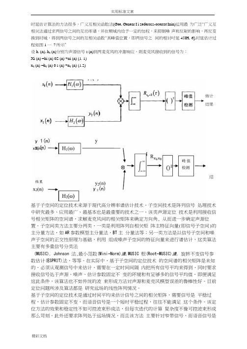
时延估计算法的方法很多，广义互相关函数法(Gee, Genear I i zedeross-ocerrat Inin)运用最为广泛"广义互相关法通过求两信号之间的互功率谱，并在频域内给予一定的加权，来抑制噪声和反射的影响，再反变换到时域，得到两信号之间的互相关函数"其峰值位置，即两信号之间的相对吋延45IH, 6],时延估计过程如图1 一7所示”设h. (n), h2 (n)分别为声源信号s (n)到两麦克风的冲激响应，則麦克风接收到的信号为：Xi (n) =hi (n) 0S (n) +ni (n) (1. 1)x2 (n) =h2 (n) 0 s (n) +n2 (n) (1.2)佈计结果结基于子空间的定位技术来源于现代高分辨率谱估计技术。

子空间技术是阵列信号处理技术中研究最多、应用最广、最基本也是最重要的技术之一。

该类声源定位技术是利用接收信号相关矩阵的空间谱，求解麦克风间的相关矩阵来确定方向角, 从而进一步确定声源位置。

子空间类方法主要分两类，一类是利用阵列自相关矩阵主特征向量(即信号子空间)的主分量方法，如AR参数模型主分量法，BT主分量法等；另一类方法是以信号子空间和噪声子空间的正交性原理为基础，利用组成噪声子空间的特征向量来进行谱估计，这类算法主要有多重信号分类法(MUSIC), Johnson 法,最小范数(Mini-Norm)法,MUSIC 根(Root-MUSIC)法, 旋转不变信号参数估计(ESPRIT)法，等等。

在实际中，基于子空间的定位技术的空间谱的相关矩阵是未知的，必须从观测信号中来估计，需要在一定时间间隔内把所有信号平均来得到，同时要求接收信号处于声源、噪声、估计参数固定不变的环境和有足够多的信号平均值。

即便满足这此条件，该算法也不如传统的波束形成方法对声源和麦克风模型误差的鲁棒性好。

目前定位问题所涉及算法都是研究远场的线性阵列情况。

基于子空间的定位技术是通过时间平均来估计信号之间的相关矩阵，需要信号是平稳过程，估计参数固定不变，而语音信号是一个短时平稳过程，往往不能满足这个条件。

Evaluation of Objective Measures for Speech Enhancement

2. Speech corpus and subjective quality evaluations
In our objective evaluations, we considered distortions introduced by speech enhancement algorithms and background noise. The list of speech enhancement algorithms considered in our study can be found in [4]. Noise was artiﬁcially added to the speech signal as follows. The Intermediate Reference System (IRS) ﬁlter used in ITU-T P.862 [5] for evaluation of the PESQ measures was independently applied to the clean and noise signals. The active speech level of the ﬁltered clean speech signal was ﬁrst determined using method B of ITU-T P.56 [6]. A noise segment of the same length as the speech signal was randomly cut out of the noise recordings taken from the AURORA database [7], appropriately scaled to reach the desired SNR level and ﬁnally added to the ﬁltered clean speech signal. A total of 16 sentences corrupted in four background noise environments (car, street, babble and train) at two SNR levels (5dB and 10dB) were processed by the 13 speech enhancement algorithms. These sentences were produced by two male and two female speakers.

开题报告6基于子空间方法的语音增强处理

[10]张雪英.数字语音处理及MATLAB仿真[M].北京:电子工业出版社, 2010.
[11]吴周桥,谈新权.基于子空间方法的语音增强算法研究[J].声学与电子工程, 2005.
指导教师批阅意见
指导教师(签名)：年月日
注：可另附A4纸
[5] K. K. Paliwal, A. Basu. A speech enhancement based on Kalman filtering[J]. Proc. ICASSP, pp. 177-180, Dec. 1987.
[6] Y. Ephraim, H. L. Van Trees. A signal subspace approach for speech enhancement[J]．IEEE Trans Speech and Audio Processing，Vol. 3,no. 4,pp. 251-266,Dec.1995.
[3] R. J. Mcaulay, M. L. Malpass. Speech enhancement using a soft-decision noise suppression filter[J]. IEEE Trans. Acoust, Speech, Signal Processing, Vol. ASSP-28, no. 2, pp. 137-145, Dec.1980.
[4] Y. Ephraim, D. Malah. Speech enhancement using a minimum mean-square error short-time spectral amplitude estimator[J]. IEEE Trans. Acoust, Speech, Signal Process, Vol. ASSP-32, no. 6, pp. 1109-1121, Dec. 1984.

摘要模板

摘要蛙人水下语音通信系统主要用于蛙人与蛙人之间、蛙人与母船或岸基之间的信息交互，其中的语音编码技术是实现语音通信的必要组成部分，为水下语音信息的顺利传输提供保障。

针对水下语音通信中遇到的水声信道的影响、水声通信技术对高速率的限制等问题，蛙人语音编码需要采用低速率语音编码技术，在有限的通信速率下实现水下的语音通信。

本文以触点传导送话器作为蛙人语音信号的采集器，分析蛙人语音信号的特性，采用混合激励线性预测(MELP)算法，实现2.4kbps 的低速率语音编码的仿真研究和在DSP 平台上的算法移植，并结合子空间语音增强技术，提高了水下语音通信系统的听觉质量。

MELP 语音编码算法具体借鉴了混合激励的形式并结合了多带的思想，本文对算法的编码和解码的基本原理进行仿真，并在TMS320C6747 DSP 平台上实现软件开发，获得的合成语音信号完整地保留了说话人的主要特征，具有良好的语音质量。

此外，本文引入触点传导送话器从信源处提高蛙人语音信号的抗干扰能力，引入子空间语音增强技术用来消除含噪信号中的噪声成分，并对线性估计器进行时域和频域上的改进，使得降噪处理的适用范围更广泛，效果更显著。

本文将MELP 语音编码技术与水声通信技术相结合，使用基于子空间的后置增强处理，在信道水池、外场水域进行了试验研究，实现了表面声道中语音信号的传输，获得了具有良好的清晰度和可懂度的合成语音，满足水下语音通信系统对语音编码的要求。

关键词：低速率语音编码；MELP；触点传导送话器；语音增强；DSPABSTRACTFrogman underwater speech communication system is mainly used to communicatebetween frogman and frogman, frogman and ship. Speech coding technology is the necessary component of this system, and guarantees the transmission of underwater speech signal successfully. For the influence of underwater acoustic channel and the limit of high data ratefor underwater acoustic communication technology, the low bit rate speech coding is neededin the limited communication rate.In this paper, frogman speech signal is acquired by contact conduction microphone, andits characteristics are analyzed. The low bit rate speech coding of 2.4kbps is achieved bymixed excitation linear prediction (MELP) algorithm, and developed in the DSP platform.The subspace-based speech enhancement is introduced to improve auditory quality of underwater speech communication. The technology of MELP speech coding has the form of mixed excitation and the idea of multiband. The basic principles of coding and encoding are simulated by MATLAB, and developed in the TMS320C6747 DSP. The results show themain characteristics of speaker are retained in the synthesized speech signal. In addition, the capability of avoiding interference of frogman speech signal is improved by contact conduction microphone, the noise component in the noisy signal is eliminated by subspace approach of speech enhancement. The constrained estimator is improved in the time and frequency domains, and the noise elimination has wider scope and more significant effect.The technologies of MELP speech coding, underwater acoustic communication andsubspace-based speech enhancement are combined, and the system is experimented in the laboratory and lake. The transmission of speech signal is achieved in the surface acoustic channel, and the results show the synthesized speech has well quality of intelligibility and clarity, which satisfies the demand of underwater speech coding.Key words: low bit rate speech coding; MELP; contact conduction microphone; speech enhancement; DSP。

Incorporating a psychoacoustical model in frequency domain speech enhancement

270IEEE SIGNAL PROCESSING LETTERS, VOL. 11, NO. 2, FEBRUARY 2004Incorporating a Psychoacoustical Model in Frequency Domain Speech EnhancementYi Hu, Student Member, IEEE, and Philipos C. Loizou, Member, IEEEAbstract—A frequency domain optimal linear estimator is proposed which incorporates the masking properties of the human auditory system to make the residual noise distortion inaudible. The use of wavelet-thresholded multitaper spectra is also proposed for frequency-domain speech enhancement methods as an alternative to the traditional fast Fourier transform (FFT)-based magnitude spectra. Experiments with multitalker babble noise indicated that the proposed estimator outperformed the minimum mean-square error log-spectral amplitude estimator (MMSE-LSA), particularly when wavelet-thresholded multitaper spectra were used in place of the FFT spectra. Index Terms—Multitaper method, musical noise, power spectrum estimation, psychoacoustical model, speech enhancement, wavelet thresholding.II. PROPOSED FREQUENCY DOMAIN SPEECH ENHANCEMENT METHOD A. Principles of Proposed Method We assume that the noise signal is additive and uncorrelated , where , and with the speech signal, i.e., are the -dimensional noisy speech, clean speech and noise vectors, respectively. By denoting the -point discrete Fourier transform matrix by , the Fourier transform of the noisy speech vector can then be written as , where and are the vectors containing the spectral components of the clean speech vector and the noise vector , respectively. be the linear estimator of , where is Let matrix. The error signal obtained in this estimation a , where is given by represents the spectrum of the speech distortion and represents the spectrum of the residual noise. Next, we define the energy of the frequency domain speech distortion as and the th spectral component of the residual noise as , where is a selector choosing the th and is defined as component ofI. INTRODUCTIONTHE KNOWN phenomenon of auditory masking has been successfully applied and used in wideband audio coding. In an effort to make the residual noise perceptually inaudible, more speech enhancement methods today are exploiting the auditory masking properties [1]–[4]. In the subtractive-type approach proposed by Virag [1], for instance, a psychoacoustical model was used to guide the derivation of the spectral subtractive parameters. Heuristic rules were used in [2] to derive spectral subtractive equations that incorporated masking thresholds. A simplified constrained minimization approach was used in [3] to derive a spectral weighting rule which was a function of the masking thresholds. In most of the above speech enhancement methods, the incorporation of auditory masking was done heuristically. This letter formulates speech enhancement in the frequency domain as a constrained minimization problem and includes the masking thresholds as the constraints. The psychoacoustical model is thereby integrated in the derived spectral weighting function. We further investigate the importance of using good (low variance) spectrum estimators in speech enhancement. This letter is organized as follows. In Section II, the proposed approach is described. Implementation details are presented in Section III, experimental results are given in Section IV, and the conclusions are given in Section V.The proposed linear estimator minimizes the frequency domain speech distortion subject to constraints on components of the spectrum of the residual noise. More specifically, we require be smaller than or equal to some that the spectral energy of , for . As we will preset threshold show later, these thresholds can be set equal to the masking thresholds. The estimator is obtained by solving the following constrained optimization problem:subject to(1)Manuscript received March 31, 2002; revised June 4, 2003. This work was supported in part by the National Institute of Deafness and Other Communication Disorders/National Institutes of Health (NIDCD/NIH) under Grant R01 DC03421. The associate editor coordinating the review of this manuscript and approving it for publication was Dr. See-May Phoong. The authors are with Department of Electrical Engineering, University of Texas at Dallas, Richardson, TX 75083-0688 USA (e-mail: yihuyxy@; loizou@). Digital Object Identifier 10.1109/LSP.2003.821714. where Problem (1) is a convex programming problem, and its solution can be found using the method of Lagrangian multipliers. Specifically, is a stationary feasible point if it satisfies the gradient equation of the objective function (2) and for (3)1070-9908/04$20.00 © 2004 IEEEHU AND LOIZOU: INCORPORATING A PSYCHOACOUSTICAL MODEL IN FREQUENCY DOMAIN SPEECH ENHANCEMENT271where is the th Lagrangian multiplier for the constraint on the th component of . From we have (4)Plugging (6) into the above equation, with the condition that , can be obtained byIn terms of the a priori SNR, Let diag be a diagonal matrix defined as , then the above equation can be rewritten ascan also be expressed as(7) (5) To simplify matters, we assume that is a diagonal matrix, i.e., we assume that the gain is applied to each frequency component and are asympindividually. The matrices and are Toeplitz) totically diagonal [5] (assuming that and are and the diagonal elements of the power spectrum components and of the clean speech vector and noise vector , respectively. Denoting the th diagonal element of by , (5) can be rewritten as for The gain function therefore obtained by for the th frequency component is Now, plugging the above equation into (6), as can be rewritten(8)It is clear from the above equation, that if the spectrum of the residual noise falls below the masking threshold, the gain is set to 1, i.e., no attenuation is performed since the th residual noise spectral component is masked. It should be noted that a similar gain function was derived in [3] using a simplified constrained minimization approach. Unlike our method, their approach was heuristic and was not based on the minimization of an error criterion. III. IMPLEMENTATION The computation of the spectral weighting function in (8) is critical for the performance of the proposed algorithm. It depends largely on accurate estimation of the clean speech spectrum and the noise spectrum. In the following sections, we discuss the computation of the clean and noise spectra. A. Spectrum Estimation Pilot informal listening tests indicated that the computation of is sensitive to the type of spectrum estimator used. In this letter, we focused on finding spectrum estimators that have low variance. More specifically, we considered using the multitaper method proposed by Thomson [7] for spectrum estimation. To further refine the spectrum estimate, the log multitaper spectrum is wavelet thresholded as in [8]. The multitaper spectrum estimator of a signal vector is given by (9) with (10) where is the number of tapers, and is the th data taper . These tapers are chosen used for the spectral estimate(6) where is defined as the a priori SNR at frequency . The above equation reduces to the Wiener filter when for all . The values, in general, control the steepness of the suppression curves (spectral attenuation vs. SNR level) producing much attenuation at low SNR with large values of levels and small values of producing less attenuation. The values need therefore to be chosen carefully to avoid speech disbased on the a posteriori tortion. One possibility is to chose SNR of the th spectral component. In the following section, based on a psychoacoustic model. we show how to chose B. Incorporating a Psychoacoustical Model One can optimally select the values by exploiting the masking properties of the human auditory system. The human listener will not perceive any noise distortion as long as the power spectrum density of the distortion lies below the masking threshold (the masking thresholds can be obtained by performing critical band analysis of the speech signal [6]). If we constrain the th spectral component of the residual noise to be lower than the masking threshold, denoted as , in values that meet this frequency bin we can compute the in (1) are set equal constraint. Assuming that the constraints to the masking thresholds , and the equality in (1) is satisfied, then implies that for272IEEE SIGNAL PROCESSING LETTERS, VOL. 11, NO. 2, FEBRUARY 2004to be orthonormal, and in this letter, we chose the sine tapers proposed by Riedel and Sidorenko [9] (11) The sine tapers were shown in [9] to produce smaller local bias than the Slepian tapers [7] with roughly the same spectral concentration. It was further shown in [8] that if is chosen to and ) the logabe at least 5, for all (except near rithm of the multitaper power spectrum in (9) plus a constant can be written as the true log power spectrum with zero mean and known plus a nearly Gaussian noise denotes the digamma function. More variance [8], where is defined as specifically, if (12) then (13) The model in (13) is well suited for wavelet denoising techniques for eliminating the “noise” term and obtaining a better estimate of the log spectrum. The idea behind refining the multitaper spectrum by wavelet thresholding can be summarized in the following four steps. 1) Obtain the multitaper spectrum using (9)–(11), and calusing (12). culate 2) Apply a standard, periodic discrete wavelet transform to get the empirical DWT (DWT) out to level to at each level , where is specified in coefficients advance [10]. (the scaling coef3) Apply a thresholding procedure to ficients are kept intact). 4) Apply the inverse DWT to the thresholded wavelet coefficients to obtain the refined log spectrum. We denote the wavelet denoised multitaper spectrum as . It should be pointed out that the wavelet denoising is not done to remove the additive noise, but rather to obtain a better (lower variance) estimate of the spectrum. B. Noise Spectrum Estimation For nonstationary environments (e.g., multitalker babble) it is imperative to update the estimate of the noise spectrum very often. One such noise estimation method, which was found to work well for nonstationary environments, is the minimum-statistics method originally proposed by Martin [11] and later modified by Cohen and Berdugo [12]. Because of its simplicity, the latter method was chosen in this letter for noise spectrum tracking. The minimum tracking is based on a recursively smoothed spectrum which is estimated using first-order recursive averagingFig. 1. Comparative performance, in terms of mean MBSD and segmental SNR measures, for 60 HINT sentences corrupted by multitalker babble at 0–20 dB SNR. The + symbols indicate performance obtained with proposed method using wavelet-thresholded multitaper spectra, and the open square symbols indicate performance obtained with the proposed method using FFT magnitude spectra.factor, and is the wavelet-thresholded multitaper spectrum of the noisy speech [note that a different method was used in [12] to obtain a smoothed version of the noisy speech spectrum, in ]. The noise spectrum is obtained by tracking place of over frames using a simplified verthe minimum of sion of the minimum statistics algorithm [12]. The estimated at frame is updated according to noise spectrum (14) is a time-varying where is an averaging parameter, and is smoothing factor, the conditional signal presence probability updated as in [12]. IV. EXPERIMENTAL RESULTS The proposed estimator was applied to 32-ms duration frames of the noisy signal with 50% overlap between frames. The enhanced speech signal was combined using the overlap and add were computed from the approach. The masking thresholds using the apestimated clean signal spectrum proach outlined in [6]. The following parameter values were used in the noise spec, , , trum estimation algorithm: , and the duration of the search window for minwere used imum tracking was set to 1 s. Five tapers in multitaper spectrum estimation. Level-dependent soft thresholding was used in the wavelet thresholding procedure as described in [8], [13] with the wavelet decomposition level set to 5. For evaluation purposes, we used 60 sentences from the Hearing in Noise Test (HINT) database [14]. For nonstationary noise, we used multitalker babble (two male and two female talkers) added to the clean speech files at 0–20 dB SNR. The modified bark spectral distortion (MBSD) measure [15] andwhere is the th component of the smoothed noisy speech spectrum at frame , is a smoothingHU AND LOIZOU: INCORPORATING A PSYCHOACOUSTICAL MODEL IN FREQUENCY DOMAIN SPEECH ENHANCEMENT273the segmental SNR measures were used for evaluation of the proposed approach. The MBSD measure is an improved version of the Bark spectral distortion (BSD) [16], which was found to be highly correlated with speech quality [15]. For comparative purposes, we also implemented and evaluated the MMSE-LSA method proposed by Ephraim and Malah [17].1 In order to make a fair comparison, the same noise spectrum estimation method was used in the MMSE-LSA estimator. Finally, in order to assess the individual contribution of the spectrum estimation method, we implemented the proposed approach using the fast Fourier transform (FFT) magnitude spectra in place of the wavelet-thresholded multitaper spectra. Fig. 1 presents the mean results in terms of the MBSD and segmental SNR measures for 60 HINT sentences corrupted by the multitalker babble noise at 0–20 dB SNR. As can be seen, the proposed approach outperformed the MMSE-LSA estimator in terms of the MBSD and segmental SNR measures. The benefit in using wavelet thresholded multitaper spectra in the computation of the gain function is also evident from Fig. 1, particularly at low SNR levels (0–5 dB). Informal listening tests confirmed that the proposed method obtained better quality with significantly lower noise distortion than the MMSE-LSA speech enhancement method. V. SUMMARY AND CONCLUSION An optimal frequency domain estimator was derived based on the masking properties of the human auditory system. The use of wavelet-thresholded multitaper spectrum estimators was shown to yield better performance in low SNR levels compared to the traditional FFT-based spectrum estimators. This advantage was attributed to the lower variance associated with multitaper spectrum estimation. Experiments with multitalker babble demonstrated improved performance, in terms of objective measures, over the MMSE-LSA speech enhancement method.REFERENCES[1] N. Virag, “Single channel speech enhancement based on masking properties of the human auditory system,” IEEE Trans. Speech Audio Processing, vol. 7, pp. 126–137, Mar. 1999. [2] D. E. Tsoukalas, J. N. Mourjopoulos, and G. Kokkinakis, “Speech enhancement based on audible noise suppression,” IEEE Trans. Speech Audio Processing, vol. 5, pp. 479–514, Nov. 1997. [3] S. Gustafsson, P. Jax, and P. Vary, “A novel psychoacoustically motivated audio enhancement algorithm preserving background noise characteristics,” in Proc. IEEE Int. Conf. Acoustics, Speech, Signal Processing, 1998, pp. 397–400. [4] F. Jabloun and B. Champagne, “A perceptual signal subspace approach for speech enhancement in colored noise,” in Proc. IEEE Int. Conf. Acoustics, Speech, Signal Processing, vol. 1, 2002, pp. 569–572. [5] R. Gray, “On the asymptotic eigenvalue distribution of Toeplitz matrices,” IEEE Trans. Inform. Theory, vol. IT-18, pp. 725–730, 1972. [6] J. D. Johnston, “Transform coding of audio signals using perceptual noise criteria,” IEEE J. Select. Areas Commun., vol. 6, pp. 314–323, Feb. 1988. [7] D. J. Thomson, “Spectrum estimation and harmonic analysis,” Proc. IEEE, vol. 70, pp. 1055–1096, Sept. 1982. [8] A. T. Walden, D. B. Percival, and E. J. McCoy, “Spectrum estimation by wavelet thresholding of multitaper estimators,” IEEE Trans. Signal Processing, vol. 46, pp. 3153–3165, Dec. 1998. [9] K. S. Riedel and A. Sidorenko, “Minimum bias multiple taper spectral estimation,” IEEE Trans. Signal Processing, vol. 43, pp. 188–195, Jan. 1995. [10] S. G. Mallat, “A theory for multiresolution signal decomposition: The wavelet presentation,” IEEE Trans. Pattern Anal. Machine Intell., vol. 11, pp. 674–693, July 1989. [11] R. Martin, “Noise power spectral density estimation based on optimal smoothing and minimum statistics,” IEEE Trans. Speech Audio Processing, vol. 9, pp. 504–512, July 2001. [12] I. Cohen and B. Berdugo, “Noise estimation by minima controlled recursive averaging for robust speech enhancement,” IEEE Signal Processing Lett., vol. 9, pp. 12–15, Jan. 2002. [13] I. M. Johnstone and B. W. Silverman, “Wavelet threshold estimators for data with correlated noise,” J. R. Statist. Soc. B, vol. 59, pp. 319–351, 1997. [14] M. Nilsson, S. Soli, and J. Sullivan, “Development of the hearing in noise test for the measurement of speech reception thresholds in quiet and in noise,” J. Acoust. Soc. Amer., vol. 95, pp. 1085–1099, 1994. [15] W. Yang, M. Benbouchta, and R. Yantorno, “Performance of the modified bark spectral distortion as an objective speech quality measure,” in Proc. IEEE Int. Conf. Acoustics, Speech, Signal Processing, 1998, pp. 541–544. [16] S. Wang, A. Sekey, and A. Gersho, “An objective measure for predicting subjective quality of speech coders,” IEEE J. Select. Areas Commun., vol. 10, pp. 819–829, June 1992. [17] Y. Ephraim and D. Malah, “Speech enhancement using a minimum mean-square error log-spectral amplitude estimator,” IEEE Trans. Acoust., Speech, Signal Processing, vol. ASSP-33, pp. 443–445, 1985. [18] I. Cohen, “Optimal speech enhancement under signal presence uncertainty using log-spectral amplitude estimator,” IEEE Signal Processing Lett., vol. 9, pp. 113–116, Apr. 2002. [19] N. Kim and J. Chang, “Spectral enhancement based on global soft decision,” IEEE Signal Processing Lett., vol. 7, pp. 108–110, May 2000.1Note that several new algorithms were proposed recently (e.g., [18] and [19]) providing improvements to the MMSE-LSA estimator, however, those algorithms incorporated signal-presence uncertainty in their spectral estimator, and our proposed estimator does not. For that reason, we only compare the performance of our estimator against the performance of the MMSE-LSA estimator.。

A SUBSPACE METHOD FOR SPEECH ENHANCEMENT IN THE MODULATION DOMAIN(13)

A SUBSPACE METHOD FOR SPEECH ENHANCEMENT IN THE MODULATION DOMAINYu Wang and Mike BrookesDepartment of Electrical and Electronic Engineering,Exhibition Road,Imperial College London,UKEmail:{yw09,mike.brookes}@ABSTRACTWe present a modulation-domain speech enhancement al-gorithm based on a subspace method.We demonstrate that in the modulation domain,the covariance matrix of clean speech is rank deﬁcient.We also derive a closed-form expression for the modulation-domain covariance matrix of colored noise in each frequency bin that depends on the analysis window shape and the noise power spectral ing this,we combine a noise power spectral density estimator with an efﬁcient subspace method using a time domain constrained (TDC)estimator of the clean speech spectral envelope.The performance of the novel enhancement algorithm is evaluated using the PESQ measure and shown to outperform competit-ive algorithms for colored noise.Index Terms-speech enhancement,subspace,modula-tion domain,covariance matrix estimation1.INTRODUCTIONWith the increasing use of hands-free telephony,especially within cars,it is often the case that speech signals are con-taminated by the addition of unwanted background acoustic noise.The goal of a speech enhancement algorithm is to re-duce or eliminate this background noise without distorting the speech signal.Over the past several decades,numerous speech enhancement algorithms have been proposed includ-ing a class of algorithms,introduced in[1],in which the space of noisy speech vectors is decomposed into a signal subspace containing both speech and noise and a noise subspace con-taining only noise.The clean speech is estimated by project-ing the noisy speech vectors onto the signal subspace using a linear estimator that minimizes the speech signal distor-tion while applying either a time domain constraint(TDC) or spectral domain constraint(SDC)to the residual noise en-ergy.The enhancer in[1],which assumed white or whitened noise,was extended to cope with colored noise in[2].Differ-ent decompositions were applied in[3]to speech-dominated and noise-dominated frames since the latter do not require prewhitening.In a generalization of the approach,[4]apply a non-unitary transformation to the noisy speech vectors that simultaneously diagonalizes the covariance matrices of both speech and colored noise.There is increasing evidence that information in speech is carried by the modulation of the spectral envelopes rather than by the envelopes themselves[5,6,7].Consequently several recently proposed enhancers act in the short-time modulation domain using minimum mean-square error(MMSE)estima-tion[8],spectral subtraction[9]or Kalmanﬁltering[10,11].This paper extends the subspace enhancement approach to the modulation domain and shows that,in this domain,the normalized noise covariance matrix can be taken to beﬁxed. The remainder of this paper is organized as follows.In Sec.2 the principle of enhancement in the short-time modulation do-main is described and in Sec.3we derive the noise covariance matrix estimate in this domain.Finally in Sec.4and Sec.5 we evaluate the algorithm and give our conclusions.2.SUBSPACE METHOD IN THE SHORT-TIMEMODULATION DOMAINThe block diagram of the proposed modulation-domain sub-space enhancer is shown in Fig.2.The noisy speech y(r) isﬁrst transformed into the acoustic domain using a short-time Fourier transform(STFT)to obtain a sequence of spec-tral envelopes Y(n,k)e j✓(n,k)where Y(n,k)is the spectral amplitude of frequency bin k in frame n.The sequence Y(n,k)is now divided into overlapping windowed modu-lation frames of length L with a frame increment J giving Y l(n,k)=p(n)Y(lJ+n,k)for n=0,···,L 1where p(n)is a Hamming window.A TDC subspace enhancer is applied independently to each frequency bin within each modulation frame to obtain the estimated clean speech spec-tral amplitudes b S l(n,k)in frame l.The modulation frames are combined using overlap-addition to obtain the estim-ated clean speech envelope sequence b S(n,k)and these are then combined with the noisy speech phases✓(n,k)and an inverse STFT(ISTFT)applied to give the estimated clean speech signalˆs(r).Following[12,10]we assume a linear model in the spec-tral amplitude domainY l(n,k)=S l(n,k)+W l(n,k)(1) where S and W denote the spectral amplitudes of clean speech and noise respectively.Since each frequency bin isEUSIPCO 2013 1569743759noisy speechoverlapping frames modulation frameoverlap-addSTFTISTFTphase spectrumenhanced speechy lenhanced magnitude spectrum y (r )ˆs(r )θ(n ,k )σ2(n ,k )Y (n ,k )ˆs l ˆS(n ,k )noise estimateTDC estimatorH lDiagram modulation domainsubspace enhancer.as dir-12 in-the in 3that thethere-en-Ween-lowal-thetheusing PESQ and shown that,for colored noise,it outperforms a time-domain subspace enhancer and modulation-domain spectral-subtraction enhancer.6.REFERENCES[1]Y.Ephraim and H.L.Van Trees.A signal subspaceapproach for speech enhancement.IEEE Trans.Speech Audio Process.,3(4):251–266,July1995.[2]H.Lev-Ari and Y.Ephraim.Extension of the signal sub-space speech enhancement approach to colored noise.IEEE Signal Process.Lett.,10(4):104–106,April2003.[3]U.Mittal and N.Phamdo.Signal/noise KLT basedapproach for enhancing speech degraded by colored noise.IEEE Trans.Speech Audio Process.,8(2):159–167,March2000.[4]Y.Hu and P.C.Loizou.A generalized subspace ap-proach for enhancing speech corrupted by colored noise.IEEE Trans.Speech Audio Process.,11(4):334–341, July2003.[5]H.Hermansky.The modulation spectrum in the auto-matic recognition of speech.In Automatic Speech Re-cognition and Understanding,Proceedings.,pages140–147,December1997.[6]R.Drullman,J.M.Festen,and R.Plomp.Effect of re-ducing slow temporal modulations on speech reception.J.Acoust.Soc.Am.,95(5):2670–2680,1994.[7]C.H.Taal,R.C.Hendriks,R.Heusdens,and J.Jensen.A short-time objecitve intelligibility measure for time-frequency weighted noisy speech.In Proc.IEEE Intl.Conf.on Acoustics,Speech and Signal Processing (ICASSP),pages4214–4217,2010.[8]Kuldip Paliwal,Belinda Schwerin,and Kamil Wójcicki.Speech enhancement using a minimum mean-square er-ror short-time spectral modulation magnitude estimator.Speech Commun.,54:282–305,February2012.[9]Kuldip Paliwal,Kamil Wójcicki,and Belinda Schwerin.Single-channel speech enhancement using spectral sub-traction in the short-time modulation domain.Speech Commun.,52:450–475,May2010.[10]S.So and K.K.Paliwal.Suppressing the inﬂuenceof additive noise on the kalman gain for low residual noise speech enhancement.Speech Communication, 53(3):355–378,2011.[11]Yu Wang and Mike Brookes.Speech enhancement us-ing a robust Kalmanﬁlter post-processor in the modu-lation domain.to appear in the Proc.IEEE Intl.Conf.on Acoustics,Speech and Signal Processing(ICASSP), May2013.[12]S.Boll.Suppression of acoustic noise in speech usingspectral subtraction.IEEE Trans.Acoust.,Speech,Sig-nal Process.,27(2):113–120,April1979.[13]S.So,K.K.Wójcicki,and K.K.Paliwal.Single-channelspeech enhancement using Kalmanﬁltering in the mod-ulation domain.In Eleventh Annual Conference of the International Speech Communication Association, 2010.[14]Y.Ephraim and D.Malah.Speech enhancement usinga minimum-mean square error short-time spectral amp-litude estimator.IEEE Trans.Acoust.,Speech,Signal Process.,32(6):1109–1121,December1984.[15]Kenneth S plex stochastic processes:anintroduction to theory and application.Addison-Wesley Publishing Company,Advanced Book Program,1974.[16]F.Olver,D.Lozier,R.F.Boiszert,and C.W.Clark,edit-ors.NIST Handbook of Mathematical Functions:Com-panion to the Digital Library of Mathematical Func-tions.Cambridge University Press,2010.[17]Y.Avargel and I.Cohen.On multiplicative transfer func-tion approximation in the short-time Fourier transform domain.IEEE Signal Process.Lett.,14(5):337–340, 2007.[18]R.Martin.Noise power spectral density estimationbased on optimal smoothing and minimum statistics.IEEE Trans.Speech Audio Process.,9:504–512,July 2001.[19]T.Gerkmann and R.C.Hendriks.Unbiased MMSE-based noise power estimation with low complexity and low tracking delay.IEEE Trans.Audio,Speech,Lang.Process.,20(4):1383–1393,May2012.[20]H.J.M.Steeneken and F.W.M.Geurtsen.Descriptionof the RSG.10noise data-base.Technical Report IZF 1988–3,TNO Institute for perception,1988.[21]P.C.Loizou.Speech databases and MATLAB codec.In Speech Enhancement Theory and Practice,chapter Appendix C,pages589–599.Taylor&Francis,2007.[22]J.S.Garofolo.Getting started with the DARPA TIMITCD-ROM:An acoustic phonetic continuous speech database.Technical report,National Institute of Stand-ards and Technology(NIST),Gaithersburg,Maryland, December1988.[23]D.M.Brookes.VOICEBOX:A speech processing tool-box for MATLAB./hp/ staff/dmb/voicebox/voicebox.html,1998-2012.。

麦克风阵列基本原理英文教材

where r = |r| is the radial distance from the source, and k is the scalar wavenumber, given by 2π /λ. The spherical wave solution shows that the signal amplitude decays at a rate proportional to the distance from the source. This dependence of the amplitude on the distance has important implications for array processing algorithms when the source is in the near-ﬁeld, as will be discussed in later sections. While sound waves are typically spherical in nature, they may be considered as plane waves at a suﬃcient distance from the source, and this approximation is often used to simplify mathematical analysis. The plane wave solution in Equation 3 is expressed in terms of two variables, time and space. Due to the well deﬁned propagation of the signal, these two variables are linked by a simple relation, and thus the solution can be expressed as function of a single variable. If we formulate the plane wave solution as x(t, r) = Aej ω(t−β·r) where β = as

Procedings of the IASTED International Conference APPLIED SIMULATION AND MODELLING

Procedings of the IASTED International ConferenceAPPLIED SIMULATION AND MODELLINGSeptember3-5,2003,Marbella,SpainA time-frequency approach to blind separation of under-determinedmixture of sourcesA.MANSOURLab.E I,ENSIETA,29806Brest cedex09,(FRANCE).mansour@M.KAW AMOTODept.of Electronic andControl Systems Eng.,Shimane University,Shimane690-8504,(JAPAN)kawa@ecs.shimane-u.ac.jpC.PuntonetDepartamento de Arquitectura yTecnologia de computadores,Universidad de Granada,18071Granada,(SPAIN).carlos@atc.ugr.esABSTRACTThis paper deals with the problem of blind separation of under-determined or over-complete mixtures(i.e.more sources than sensors).Atﬁrst a global scheme to sepa-rate under-determined mixtures is presented.Then a new approach based on time-frequency representations(TFR) is discussed.Finally,some experiments are conducted and some experimental results are given.KEY WORDSICA,BSS,Time-Frequency domain,over-complete or under-determined mixtures1.IntroductionBlind separation of sources problem is a recent and an im-portant signal processing problem.This problem involves recovering unknown sources by only observing some mixed signals of them[1].Generally,researchers assume that the sources are statistically independent from each other and at most one of them can be a Gaussian signal[2]. Other assumptions can be also founded in the literature concerning the nature of the transmission channel(i.e.an instantaneous or a memoryless channel,a convolutive or a memory channel,and a non-linear channel).In addition,a widely used assumption considers that the number of sen-sors should be equal or greater(for subspace approaches) than the number of sources.These assumptions are fairly satisﬁed in many divers applications such as robotics, telecommunication,biomedical engineering,radars,etc., see[3].In recent applications linked to special scenarios in telecommunication(as satellite communication in double-talk mode),robotics(for exemple,robots which imitate human behavior)or radar(in ELectronic INTelli-gence”ELINT”applications),the assumption about the number of sensors can not be satisﬁed.In fact,in the latter applications the number of sensors is less than the number of sources and often we should deal with a mono-sensor system with two or more sources.Recently,few authors have considered the under-determined mixtures.Thus by using overcomplete repre-sentations,Lewicki and Sejnowski in[4]present an algo-rithms to learn overcomplete basis.Their algorithm uses a Gaussian approximation of probability density function (PDF)to maximize the probability of the data given the model.Their approach can be considered as a generaliza-tion of the Independent Component Analysis(ICA)[2]in the case of instantaneous mixtures.However,in this ap-proach,the sources should be sparse enough to get good ex-perimental results,otherwise the sources are being mapped down to a smaller subspace and there is necessary a loss of ing the previous approach,Lee et al.[5] separate successfully three speech signals using two micro-phones.On the other hand,When the sources are sparsely distributed,at any time t,at most one of sources could be signiﬁcantly different from zero.In this case,estimating the mixing matrix[6,7,8]consists ofﬁnding the direc-tions of maximum data density by simple clustering ing Reimannian metrics and Lie group structures on the manifolds of over-complet mixture matrices,Zhang et al.[9]present a theoretical approach and develop an al-gorithm which can be considered as a generalization of the one presented in[10].The algorithm of Zhang et al.up-date the weight matrix by minimizing a kullback-Leibler divergence by using natural learning algorithm[11].In the general case,one can consider that separation of over-complete mixtures still a real challenge for the sci-entiﬁc community.However,some algorithms have been proposed to deal with particular applications.Thus for bi-nary signals used in digital communication,Diamantaras and Chassioti[12,13]propose an algorithm based on the PDF of the observed mixed signals.The pdf of the ob-servation signals have been modeled by Gaussian pdf and estimated from the histogram of the observed -ing differential correlation function,Deville and Savoldelli [14]propose an algorithm to separate two sources from noisy convolutive mixtures.The proposed approach re-quires the sources to be long-term non-stationary signals and the noise should be long-terme stationary ones.The previous statement means that the sources(resp.noise) should have different(resp.identically)second order statis-tics at different instances separated by a long period.2.Channel ModelHereinafter,we consider that the sources are non Gaus-sian signals and statistically independent from each other.In addition,we assume that the noise is an additive whiteGaussian noise (AWGN).Letdenote the source vector at any time t,is mixing vector and is a AWGN vector.The channel is represented by a full rank real and constant matrix ().H ( )Channel+B(t)S(t)Figure 1.General structure.The separation is considered achieved when the sources are estimated up to a scale factor and a permuta-tion.That means the global matrix can be written as:here,is a weight matrix,is a permutation matrix and is a non-zero diagonal matrix.For a sake of simplic-ity and without loss of generality,we will consider in the following that:Where is an invertible matrix and is a full rankrectangular matrix.3.A Separation SchemeIn the case of over-complete mixtures (),the invert-ibility of the mixing matrix becomes an ill-conditioned problem.That means the Independent Component Analy-sis (ICA)will be reduced to extract independent signals which are not necessarily the origine sources,i.e.the sep-aration can not give a unique solution.Therefore,further assumptions should be considered and in consequence suit-able algorithms could be developed.Thus,two strategies can be considered:At ﬁrst one can identify the mixing matrix then us-ing this estimated matrix along with important infor-mation about the nature or the distributions of the sources,we should retrieve the original sources.In many applications (such as speech signals,telecom-munications,etc ),one can assume the sources havespecial features (constant modulus,frequency prop-erties,etc ).Using sources’speciﬁcs,the separation becomes possible in the classic manner,i.e.up to per-mutation and a scale factor.Beside the algorithms cited and discussed in the intro-duction of our manuscript,few more algorithms can be founded in the literature.The latter publications are dis-cussed in this section.3.1Identiﬁcation &SeparationOne of the ﬁrst publications on the identiﬁcation of under-determined mixtures was proposed by Cardoso [15].In his manuscript,Cardoso proposed an algorithm based only on fourth-order cumulant.In fact,using the symmetries of quadricovariance tensor,an identiﬁcation method based on the decomposition of the quadricovariance was proposed.Recently,Comon [16]proved using an algebraic approach,that the identiﬁcation of static MIMO (Multiple Inputs Multiple Outputs)with fewer outputs than inputs is possible.In other words,he proved that the CANonical Decomposition (CAND)of a fourth-order cross-cumulant tensor can be considered to achieve the identiﬁcation.In addition,he proved that ICA is a symmetric version of ing a Sylveter’s theorem in multilinear algebra and the fourth order cross cumulant tensor,he proposed an algorithm to identify the mixing matrix in the general case.To recover d-psk sources,comon proposes alsoa non-linear inversion ofby adding some non-linear equations and using the fact that the d-psk signals satisfyspecial polynomial properties (i.e.).Later on,Comon and Grellier [17]proposed an extension of the previous algorithm to deal with different communication signals (MSK,QPSK and QAM4).Similar approach was also proposed by De Lathauwer et al.,see [18].Finally,Taleb [19]proposes a blind identiﬁcation al-gorithm of M-inputs and 2-outputs channel.He proved thatthe coefﬁcients of the mixing matrixare the roots of a polynomial equations based on the derivative of the sec-ond characteristic function of the observed signals.The uniqueness of the solution is proved using Darmois’Theo-rem [20].3.2Direct SeparationHere,we discuss methods to separate special signals.As it is mentioned in the previous subsection that Comon et al.[16,17]proposed an algorithm to separate communication signals.Nakadai et al.[21,22]addressed the problem of a blind separation of three mixed speech signals with the help of two microphones by integrating auditory and vi-sual processing in real world robot audition systems.Theirapproach is based on direction pass-ﬁlters which are imple-mented using the interaural phase difference and the inter-aural intensity difference in each sub-band -ing Dempster-Shafer theory,they determine the direction of each sub-band frequency.Finally,the waveform of one sound can be obtained by a simple inverse FFT applied to the addition of the sub-band frequencies issued by the spe-ciﬁc direction of that speaker.Their global system can per-form sound source localization,separation and recognition by using audio-visual integration with active movements.4.Time-Frequency ApproachThe algorithm proposed in this section is based on time-frequency distributions of the observed signals.To our knowledge,few time-frequency methods have been devoted to the blind separation of MIMO channel.In fact,for MIMO channel with more sensors than sources, Belouchrani and Moeness[23]proposed a time-frequency separation method exploiting the difference in the time-frequency signatures of the sources which are assumed to be nonstationary multi-variate process.Their idea consists on achieving a joint diagonalization of a combined set of spatial time-frequency distributions which have been deﬁned in their paper.It is clear from the discussion of the previous sections that the identiﬁcation of MIMO channel is possible.How-ever,the separation is not evident in the general case.The few published algorithms for the under-determined matter are very linked to signal features of theirs applications.In our applications,an instantaneous static under-determined mixture of speech signals is considered.This problem can be divided into two steps:Atﬁrst an identiﬁcation algorithm should be applied.For the moment,we didn’t develop a speciﬁc identi-ﬁcation algorithm.Therefore,any identiﬁcation algo-rithms previously mentioned can be used.Let us assume that the coefﬁcient of the mixing matrixhave been estimated.The question becomes How can we recover the sources from fewer sensors?To answer this question,we consider in this section the separation of a few speech signals(for the instance, we are considering just two or at most three sources) using the output of a single microphone(i.e.Multiple Inputs Single output,MISO channel).Recently,time-frequency representations(TFR) have been developed by many researchers[24]and they are considered as very powerful signal processing tools.In the literature,many different TFR have been developed as Wigner-Ville,Pseudo-Wigner-Ville,Smooth Pseudo-Wigner-Ville,Cho-Willims,Born-Jordan,etc.In a previous study[25],we found that for simplicity and performance reasons,the Pseudo-Wigner-Ville can be considered as a good TFR candidate.Here we present a new algorithm based on time-frequency representations of the observed signals(TFR)to separate a MISO channel with speech sources.It is known that speech signals are non-stationary signals.However within phonemes(about80ms of duration)the statistics of the signal are relatively constant[26].On the other hand,It is well known that voiced speech are quasi-periodic signals and the non-voiced signals can be considered as white ﬁltered noise[27].Within a small window corresponding to51ms,the pitch can be slightly change.Therefore,one can use this property to pick up the frequency segments of a speaker.The pitch can be estimated using divers techniques[28].Using the previous facts and Pseudo-Wigner-Ville representations,one can separate up to three speech signals from one observed mixed signal of them.To achieve that goal,we assume that the time-frequency signatures of the sources are disjoints.Atﬁrst,one should calculate the TFR of the observed signal.Then,in the time-frequency space, we plot a regular grilled.The dimensions of the a small cell of the grilled are evaluated based on the properties of the speech signals and the sampling frequency.Therefore, these dimensions can be considered as10to20ms in length (i.e.time axis)and5to10%of the sampling frequency value in the vertical axis.Once we plot the grilled,we estimate the energy average in each cell and a threshold is applied to distinguish noisy cells from other.Then the cell with the maximum energy is considered as a potential pitch of one speaker and it is pointed out.After that,we merge in a set of cells,all cells with high level of energy in the neighborhood of the previous cell.At least one har-monic of the pitch should be also selected.The previous steps should repeated as necessary.Finally,the obtained map can be considered as a bi-dimensional time-frequency ﬁlters which should be applied on the mixed -ing a simple correlation maximization algorithm,one can ﬁnd the different pieces corresponding to the speech of one speaker.5.Experimental ResultsTo demonstrate the validity of the proposed algorithm men-tioned in section4,many computer simulations were con-ducted.Some results are shown in this section.We consid-ered the following two-input and one-output system.(1)The sources were male and female voices which were recorded by8[KHz]sampling fre-quency.The TFR was calculated by using128data of the observed signal.Figure2shows the results obtained by applying the proposed algorithm(last paragraph in section4)to the ob-served signal.From thisﬁgure,one might think that the estimated signals are different from the original signals. However,if one hear the estimated signals,one can see that the two original sources and are separated from the observed signal by the proposed algorithm.6.ConclusionThis paper deals with the problem of blind separation of under-determined(or over-complete)mixtures(i.e.more sources than sensors).Atﬁrst,a survey on blind separation algorithms for under-determined mixtures is given.A sep-aration scheme based on identiﬁcation or direct separation is discussed.A new time-frequency algorithm to separate speech signals has been proposed.Finally,some experi-ments have been conducted and the some experimental re-sults are given.Actually,we are working on a project con-cern the separation of under-determined mixtures.Further results will be the subject of future communications.References[1]A.Mansour, A.Kardec Barros,and N.Ohnishi,“Blind separation of sources:Methods,assumptions and applications.,”IEICE Transactions on Funda-mentals of Electronics,Communications and Com-puter Sciences,vol.E83-A,no.8,pp.1498–1512, August2000.[2]on,“Independent component analysis,a newconcept?,”Signal Processing,vol.36,no.3,pp.287–314,April1994.[3]A.Mansour and M.Kawamoto,“Ica papers classi-ﬁed according to their applications&performances.,”IEICE Transactions on Fundamentals of Electronics, Communications and Computer Sciences,vol.E86-A,no.3,pp.620–633,March2003.[4]M.Lewicki and T.J.Sejnowski,“Learning non-linear overcomplete representations for efﬁcient cod-ing,”Advances in neural Information Processing Sys-tems,vol.10,pp.815–821,1998.[5]T.W.Lee,M.S.Lewicki,M.Girolami,and T.J.Se-jnowski,“Blind source separation of more sources than mixtures using overcomplete representations,”IEEE Signal Processing Letters,vol.6,no.4,pp.87–90,April1999.[6]P.Boﬁll and M.Zibulevsky,“Blind separation ofmore sources than mixtures using sparsity of their short-time fourier transform,”in International Work-shop on Independent Component Analysis and blind Signal Separation,Helsinki,Finland,19-22June 2000,pp.87–92.[7]P.Boﬁll and M.Zibulevsky,“Underdetermined blindsource separation using sparse representations,”Sig-nal Processing,vol.81,pp.2353–2363,2001. [8]P.Boﬁll,“Undetermined blind separation of delayedsound sources in the frequency domain,”NeuroCom-puting,p.To appear,2002.[9]L.Q.Zhang,S.I.Amari,and A.Cichocki,“Nat-ural gradient approach to blind separation of over-and under-complete mixtures,”in First International Workshop on Independent Component Analysis and signal Separation(ICA99),J.F.Cardoso,Ch.Jutten, and Ph.loubaton,Eds.,Aussois,France,11-15Jan-uary1999,pp.455–460.[10]M.Lewicki and T.J.Sejnowski,“Learning overcom-plete representations,”Neural Computation,vol.12, no.2,pp.337–365,2000.[11]S.I.Amari,A.Cichocki,and H.H.Yang,“A newlearning algorithm for blind signal separation,”in Neural Information Processing System8,Eds.D.S.Toureyzky et.al.,1995,pp.757–763.[12]K.Diamantaras and E.Chassioti,“Blind separationof n binary sources from one observation:A deter-ministic approach,”in International Workshop on In-dependent Component Analysis and blind Signal Sep-aration,Helsinki,Finland,19-22June2000,pp.93–98.[13]K.Diamantaras,“Blind separation of multiple binarysources using a single linear mixture,”in Proceed-ings of International Conference on Acoustics Speech and Signal Processing2001,ICASSP2000,Istanbul, Turkey,Jun2000,pp.2889–2892.[14]Y.Deville and S.Savoldelli,“A second order dif-ferential approach for underdetermined convolutive source separation,”in Proceedings of International Conference on Acoustics Speech and Signal Process-ing2001,ICASSP2001,Salt Lake City,Utah,USA, May7-112001.[15]J.F.Cardoso,“Super-symetric decomposition of thefourth-order cumulant tensor.blind identiﬁcation of more sources than sensors.,”in Proceedings of Inter-national Conference on Speech and Signal Process-ing1991,ICASSP’91,Toronto-Canada,May1991, pp.3109–3112.[16]on,“Blind channel identiﬁcation and extrac-tion of more sources than sensors,”in In SPIE Confer-ence on Advanced Algorithms and Architectures for Signal Processing,San Diego(CA),USA,July19-24 1998,pp.2–13,Keynote address.[17]on and O.Grellier,“Non-linear inversion ofunderdetermined mixtures,”in First International Workshop on Independent Component Analysis andFigure2.Simulations Results:(a)Source signal(b)Source signal(c)Observed signal(d)Estimated signal of(e)Estimated signal ofsignal Separation(ICA99),J.F.Cardoso,Ch.Jut-ten,and Ph.loubaton,Eds.,Aussois,FRANCE,11-15 January1999,pp.461–465.[18]L.De Lathauwer,on,B.De Moor,and J.Van-dewalle,“ICA algorithms for3sources and2sen-sors,”in IEEE SP Int Workshop on High Order Statis-tics,HOS99,Caeserea,Israel,12-14June1999,pp.116–120.[19]A.Taleb,“An algorithm for the blind identiﬁcation ofn independent signals with2sensors,”in Sixth Inter-national Symposium on Signal Processing and its Ap-plications(ISSPA2001),M.Deriche,Boashash,and W.W.Boles,Eds.,Kuala-Lampur,Malaysia,August 13-162001.[20]G.Darmois,“Analyse g´e n´e rale des liaisons stochas-tiques,”Rev.Inst.Intern.Stat.,vol.21,pp.2–8,1953.[21]K.I.Nakadai,K.Hidai,H.G.Okuno,and H.ki-tano,“Real-time speaker localization and speech sep-aration by audio-visual integration,”in17th inter-national Joint Conference on Artiﬁcial Intelligence (IJCAI-01),Seatle,USA,August2001,pp.1425–1432.[22]H.G.Okuno,K.Nakadai,T.Lourens,and H.kitano,“Separating three simultaneous speeches with two microphones by integrating auditory and visual pro-cessing,”in European Conference on Speech Process-ing,Aalborg,Denmark,September2001,pp.2643–2646.[23]A.Belouchrani and M.G.Amin,“Blind source sep-aration based on time-frequency signal representa-tions,”IEEE Trans.on Signal Processing,vol.46, no.11,pp.2888–2897,1998.[24]P.Flandrin,Time-Frequency/Time-Scale analysis,Academic Press,Paris,1999.[25]D.Le Guen and A.Mansour,“Automatic recogni-tion algorithm for digitally modulated signals,”in6th Baiona workshop on signal processing in communi-cations,Baiona,Spain,25-28June2003,p.To ap-pear.[26]J.Thiemann,Acoustic noise suppression for speechsignals using auditory masking effects,Ph.D.thesis, Department of Electrical&Computer Engineering, McGill University,Canada,July2001.[27]R.Le Bouquin,Traitemnet pour la reduction du bruitsur la parole application aux communications radio-mobiles.,Ph.D.thesis,L’universit´e de Rennes I,July 1991.[28]A.Jefremov and B.Kleijn,“Sline-based continuous-time pitch estimation,”in Proceedings of Interna-tional Conference on Acoustics Speech and Signal Processing2002,ICASSP2002,Orlando,Florida, U.S.A,13-17May2002.。

声学中srbw 的意思

声学中srbw 的意思英文回答：SRBW stands for Speech Recognition by Waveform. It is a technique used in acoustic signal processing for speech recognition. In SRBW, the speech signal is analyzed by extracting various features from the waveform, such as pitch, intensity, and spectral content. These features are then used to train a machine learning model, such as a Hidden Markov Model (HMM), to recognize and classify different speech patterns.One example of SRBW is the use of Mel-frequency cepstral coefficients (MFCCs) as the feature extraction technique. MFCCs are a representation of the short-term power spectrum of a sound, based on a linear cosine transform of the logarithm of the power spectrum. By extracting MFCCs from the speech waveform, we can capture important information about the spectral content of the speech signal.To illustrate the use of SRBW, let's say we want to build a speech recognition system for a virtual assistant. We can collect a dataset of spoken commands, such as "play music", "set an alarm", and "send a message". We then extract features from the waveform of these spoken commands using SRBW techniques, such as MFCCs. We can use these features to train a machine learning model to recognize and classify the spoken commands.Once the model is trained, we can use it to recognize spoken commands in real-time. For example, when a user says "play music", the speech signal is processed using SRBW techniques to extract features, which are then fed into the trained model. The model then predicts the spoken command, and the virtual assistant can take appropriate actions, such as playing music.中文回答：SRBW是声学信号处理中的一种技术，全称为Speech Recognition by Waveform（声波语音识别）。

基于相空间重构的语音增强

(天津大学电子信息工程学院, 天津, 300072)
摘要: 将相空间降噪方法应用于语音增强之中。由于语音信号集中在有限空间, 而随机噪声则分散在各个分量中, 通过找到信号能量集中的信号空间, 去除噪声能量集中的冗余空间, 达到减少噪声的目的。针对语音信号的特点, 本文对相空间降噪基本算法中邻点的选取方法进行了改进, 在没有增加太多运算量的前提下, 提高了对不同信噪比信号的适应性。另外, 应用改进后的算法, 本文分别对汉语单个音素和连续语音进行了相空间语音增强测试。实验结果显示, 改进邻域选择后的相空间语音增强方法可以显著提高信噪比。关键词: 语音增强; 相空间重构; 相空间降噪中图分类号: TN 912. 35 文献标识码:A
[ 12 3]
1 相空间重构及 Ta ken s 定理
常见的混沌信号降噪算法有相空间重构、小波降噪、扩展卡尔曼滤波器降噪、正反向迭代降噪和神经网络建模等方法 [4 ] , 其中基于相空间重构的方法应用最为普遍。最初提出相空间重构的目的在于在高维相空间中恢复混沌吸引子。混沌吸引子作为混沌系统的特征之一 , 体现着混沌系统的规律性, 意味着混沌系统最终会落入某一特定的轨迹之中 , 这种特定的轨迹就是混沌吸引子。文献 [5 ] 建议用原始系统中的某变量的延迟坐标来重构相空间, 文献 [ 6 ] 的 Takens 定理证明了可以找到一个合适的嵌入维 ,
引言
语音增强的研究目的主要是如何尽量减少被噪声污染的语音信号中的噪声成分, 并尽量减小语音信号的失真度, 增加其可懂度和舒适度。语音信号可以看作短时平稳信号 , 常用的语音增强方法有: 噪声对消法、谐波增强法、基于语音生成模型的增强算法和基于短时谱估计的增强算法等。此外, 语音信号也具有混沌学特征

大学英语四级词汇活记活用（第二十六期）

A language is a signaling system which operates with symbolic vocal sounds (语声), and which is used by a group of people for the purpose of communication. Let’s look at this __1__ in more detail because it is language, more than anything else, __2__ distinguishes man from the rest of the __3__ world. Other animals, it is true, communicate with one another by __4__ of cries: for example, many birds utter __5__ calls at the approach of danger; monkeys utter __6__ cries, such as expressions of anger, fear and pleasure. __7__ these various means of communication differ in important ways __8__ human language. For instance, animals’ cries do not __9__ thoughts and feelings clearly. This means, basically, that they lack structure. They lack the kind of structure that __10__ us to divide a human utterance into __11__. We can change an utterance by __12__ one word in it with __13__: a good illustration of this is a soldier who can say, e.g., “tanks approaching from the north“, __14__ who can change one word and say aircraft approaching from the north” or “tanks approaching from the west”; but a bird has a single alarm cry, __15__ means “danger!” This is why the number of __16__ that an animal can make is very limited: the great tit (⼭雀) is a case __17__ point; it has about twenty different calls, __18__ in human language the number of possible utterances is __19__. It also explains why animal cries are very __20__ in meaning. 1.A) classification B) definition C) function D) perception 2.A) that B) it C) as D) what 3.A) native B) human C) physical D) animal 4.A) ways B) means C) methods D) approaches 5.A) mating B) exciting C) warning D) boring 6.A) identical B) similar C) different D) unfamiliar 7.A) But B) Therefore C) Afterwards D) Furthermore 8.A) about B) with C) from D) in 9.A) infer B) explain C) interpret D) express 10.A) encourages B) enables C) enforces D) ensures 11.A) speeches B) sounds C) words D) voices 12.A) replacing B) spelling C) pronouncing D) saying 13.A) ours B) theirs C) another D) others 14.A) so B) and C) but D) or 15.A) this B) that C) which D) it 16.A) signs B) gestures C) signals D) marks 17.A) in B) at C) of D) for 18.A) whereas B) since C) anyhow D) somehow 19.A) boundless B) changeable C) limitless D) ceaseless 20.A) ordinary B) alike C) common D) general 1,When I was very young, I was terribly frightened of school, but I soon______________(克服了这种⼼理). 2,Please don’t stand in the kitchen, you’re________________（挡路了）. 3,How close parents are to their children_________________ __(有很强的影响) the character of the children. 4,Mark often____________________________(试图逃脱罚款) whenever he breaks traffic regulations. 5,In the Chinese household, grandparents and other relatives_____________(起着不可缺少的作⽤) in raising children. 答案解析：1. C2. A3. D4. B5. C6. C7. A8. C9. D 10. B 11. C 12. A 13. C 14. B 15. C 16. C 17. A 18. A 19. C 20. D 1,语境题.本题的解答需要对⽂章的第⼀段进⾏理解.第⼀段主要讲到了声⾳的作⽤,注意到本句中的more detail,即更多的细节,这说明本句话是对上⼀段的补充说明,所以应该选择表⽰作⽤意思的function. 2,语法题.分析本句话Let’s look at this __1__ in more detail because it is language, more than anything else, __2__ distinguishes man from the rest of the __3__ world.将本句中的主句及插⼊结构拿开不管,本题所考察的句⼦应该是it is language__2__ distinguishes man from the rest of the __3__ world.分析可知本句话是⼀个强调句.由此本题应该选择that. 3,词汇搭配题.分析本句话it is language, more than anything else, __2__ distinguishes man from the rest of the __3__ world.本句话的意思是是语⾔,⽽不是别的什么东西,把⼈和...世界区别开来.考察四个选项,根据常理,应该选择animal,即动物世界. 4,词汇搭配题.本题主要考查的是固定搭配by means of...意思为以...⽅式.⽽其他三个词语的搭配为:way ＋ to do/of doing sth. ,method ＋of,approach to＋名词.这四个词组都表⽰...的⽅法,⽅式的意思. 5,语境题.分析本句话many birds utter __5__ calls at the approach of danger.由句中的标志词danger可知应该选择warning. 6,语境题.分析本句话monkeys utter __66__ cries, such as expressions of anger, fear and pleasure.猴⼦的叫声所表达的是⽣⽓,恐惧,⾼兴三种情绪,所以应该选择different. 7,语境题.本题考查两句话之间的逻辑关系.前⼀个句⼦讲鸟和猴⼦⽤叫声表达情绪,后⼀个句⼦讲交流的多种⽅法在⽅式上不同于⼈类的语⾔. 8,词汇搭配题.本题考查固定搭配differ...from...意思为与...不同. 9,语境题.本题运⽤复现结构的⽅法解题.在前⾯已经提到monkeys utter different cries, such as expressions of anger, fear and pleasure.本句中animals’ cries do not __9__ thoughts and feelings clearly.前⾯讲猴⼦⽤不同的叫声表达⽣⽓,恐惧,⾼兴,这⼀句⼜讲动物的叫声不能清楚的...想法和感觉.由此可知应该选择表达的动词形式express. 10,词汇搭配题.本题所填词汇需要满⾜两个条件,⾸先满⾜结构*(动词) sb.to do sth.,另外要符合上下⽂的意思.由此可以确定应该选择enable,enable sb.to do sth.的意思是使某⼈能... 11,语境题.分析本句话divide a human utterance into __11__.意思是将⼈类语⾔划分为...,由divide...into...这个词组可以知道所填⼊的词语与human utterance是相关的词语.考察四个选项,speech的意思是说话,说话⽅式或演讲,由此可以排除该选项,因为两者意思相同.sound的意思是声⾳,word的意思是字,话,消息,词,诺⾔,命令,代码,voice的意思是声⾳,由此可以确定应该选择word. 12,语境题.本题应⽤到复现结构解答本题.分析本句话,We can change an utterance by __12__ one word in it with __13__,由by引导的部分是⽂章的⽅式状语,其实是与主句所表达意思是相近的.根据主句中的词语change,可以确定应该选择与其意思相近的replace,意思为代替. 13,搭配题.⾸先分析句⼦We can change an utterance by __12__ one word in it with __13__,注意到⽂章中的one word,并且分析后⾯的内容可知,后⾯主要是讲⼈们的某⼀表达中,⽤⼀个词语代替另⼀个词语.由one可知,本题答案为another,即另⼀个. 14,语境题.本题是考查两句话之间的逻辑关系.分析句⼦a good illustration of this is a soldier who can say, e.g., “tanks approaching from the north“, __14__ who can change one word and say aircraft approaching from the north”句中含有两个并列的定语从句,⽽两个从句之间的意思是相近的,所以应该选择and. 15,语法题.本题考查⾮限定性定语从句.分析句⼦a bird has a single alarm cry, __75__ means “danger!”由句中的逗号,以及句⼦的结构可以判断出是⾮限定性定语从句,由此可以确定选择which. 16,语境题.分析本句话,This is why the number of __16__ that an animal can make is very limited.本题所要求填⼊的词语是定语从句的先⾏词,由定语从句分析可知,从句所表达的意思与⽂章第⼆段所表达的动物的特殊的表达⽅式很有限意思是相同的.所以本题应该选择符合⽂章意思的表⽰动物特殊的表达⽅式,也就是信号的意思,由此确定选择signal. 17,词汇搭配题.本题考查固定搭配in point,意思为相关的,适⽤的. 18,语境题.本句主要考查两个句⼦之间的逻辑关系.分析本句话it has about twenty different calls, __18__ in human language the number of possible utterances is __19__.由分析可知,前半句是讲⼤⼭雀的,后半句话是将⼈的,本⽂的⼤意就是⽐较⼈类和动物语⾔的区别.由此可以确定选择表⽰然⽽意思的whereas. 19,语境题.本题的解答需要理解本⽂的⼤意.本⽂主要讲动物的语⾔表达很有限,只能表达笼统的意思,⽽⼈类的语⾔很丰富,可以表达特定的意思.⽽本句前半句讲⼤⼭雀的20种叫声,⽽含半句是与前半句形成强对⽐的,所以应该选择含有⽆限的意思的limitless. 20,语境题.本句话是⽂章的最后⼀句话,⼜总结全⽂的意思.所以本题的解答依旧需要根据全⽂的⼤意来解题.由上⼀题分析可知⼈的语⾔可以表达具体特定的意思,⽽动物发出了声⾳只能表达笼统的意思.所以本题应该选择general. 1,overcame it/got over it 2,in the way 3,has a strong influence on 4,attempts to escape being fined 5,play indispensable roles。

1、下载文档前请自行甄别文档内容的完整性，平台不提供额外的编辑、内容补充、找答案等附加服务。
2、"仅部分预览"的文档,不可在线预览部分如存在完整性等问题,可反馈申请退款(可完整预览的文档不适用该条件!)。
3、如文档侵犯您的权益，请联系客服反馈,我们会尽快为您处理(人工客服工作时间：9:00-18:30)。