北京大学CCER-中级微观经济学-尼克尔森教材课后习题答案 综述
中级微观经济学习题答案
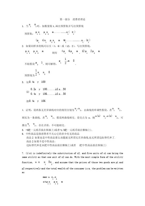
第一部分 消费者理论1. 当11xx 时,加数量税t,画出预算集并写出预算线预算集:).....(. (1)12211x x m x p x p).........(..........)(1112211x x x t m x p x t p2. 如果同样多的钱可以买(4,6)或(12,2),写出预算线。
mx p x p 2211 则有mp p 2164,mp p 21212不妨假设12 p ,则可解得:8,211 m p 。
预算线为82121 x x 3.(1)0.4100x y(2)0.2100.............300.4106.............30x y if x x y if x(3)0.4106x y4. 证明:设两条无差异曲线对应的效用分别为21,uu ,由曲线的单调性假设,若21uu ,则实为一条曲线。
若21uu ,假设两曲线相交,设交点为x,则21)(,)(ux u u x u ,可推出21uu ,存在矛盾,不可能相交。
5. -5(把一元纸币放在纵轴上)或者-1/5(把一元纸币放在横轴上),6. 中性商品是指消费者不关心它的多少有无的商品商品2 如果也是中性商品那么该题就无所谓无差异曲线,也无所谓边际替代率了. 商品2如果不是中性商品:边际替代率是0(把中性商品放在横轴上)或者 (把中性商品放在纵轴上)7. (1)x1 is indefinitely the substitution of x2, and five units of x1 can bring the same utility as that one unit of x2 can do. With the most simple form of the utilityfunction,125u x x x , and assume that the prices of those two goods are p1 and p2 respectively and the total wealth of the consumer is m, the problem can be writtenas121112max ,..u x xst p x p x m③ Because 5p1=p2, any bundle 12,x x which satisfies the budget constraint, is thesolution of such problem.(2) A cup of coffee is absolutely the complement of two spoons of sugar. Let x1 and x2 represent these two kinds of goods, then we can write the utility function as12121,min ,2u x x x xThe problem of the consumer is121112max ,..u x xst p x p x mAny solution should satisfies the rule that 1212x x , and the budget constraint.So replace x1 with (1/2)(x2) in the budget constraint and we can get 1122mx p p,and 21222mx p p.8. (1) Because the preference is Cobb-Douglas utility, we can simplify thecomputation by the formula that the standardized parameter of one commodity means its share of total expenditure.So directly, the answer is 1123m x p , 213mx p.(详细方法见8(2)). (2)库恩-塔克定理。
中级微观经济学习题解答最终版5资料讲解
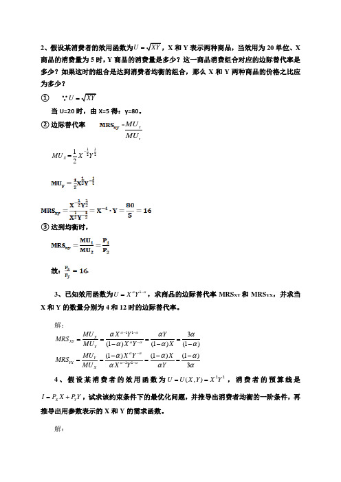
2、假设某消费者的效用函数为U XY =,X 和Y 表示两种商品,当效用为20单位、X 商品的消费量为5时,Y 商品的消费量是多少?这一商品消费组合对应的边际替代率是多少?如果这时的组合是达到消费者均衡的组合,那么X 和Y 两种商品的价格之比应为多少?① ∵U XY =当U=20时,由X=5得:y=80。
② 边际替代率Y X MU MU11221=2X MU X Y -③ 达到均衡时,故:. 3、已知效用函数为1U X Y αα-=,求商品的边际替代率MRS XY 和MRS YX ,并求当X 和Y 的数量分别为4和12时的边际替代率。
解:11113(1)(1)(1)(1)(1)(1)3X XY Y Y YX X MU X Y Y MRS MU X Y X MU X Y X MRS MU X Y Y αααααααααααααααααααα------====------====4、假设某消费者的效用函数为22(,)U U X Y X Y ==,消费者的预算线是X Y I P X P Y =+,试求该约束条件下的最优化问题,并推导出消费者均衡的一阶条件,再推导出用参数表示的X 和Y 的需求函数。
解:22max ..X Y U X Y s t I P X P Y ⎧=⎨=+⎩ 22()X Y L X Y I P X P Y λ=+--220X L XY P Xλ∂=-=∂……(1) 220Y L X Y P Yλ∂=-=∂……(2) 0X Y L I P X P Y λ∂=--=∂……(3) (1)除于(2)可得:X YP Y X P =……(4) 由(4)得:X YP Y X P =……(5) 将(5)代入(3)得:2XI X P =……(6) 将(6)代入(5)得: 2Y I Y P =……(7) 答:(4)式为一阶条件,(6)、(7)式为需求函数。
5、一个消费者每期收入为192元,他有两种商品可以选择:商品A 和B ,他对两种商品的效用函数为U AB =,PA 为12元,PB 为8元。
(完整版)中级微观经济学第七次习题参考答案最终版
《中级微观经济学》第七次习题参考答案1. 请判断下列说法的对错,并简要说明理由。
(1)在囚徒困境中,如果每一个囚犯都相信另一个囚犯会抵赖,那么两个人都会抵赖。
【答案】错误,在单期博弈中,无论另一个囚犯招供不招供,这个囚犯都会招供,招供是其占优策略。
在无限重复博弈中,所有个体理性点都可能构成纳什均衡。
(2)因为零和博弈中博弈方之间的关系都是竞争性的、对立的,因此零和博弈就是非合作博弈。
【答案】错误。
非合作博弈是指各个成员单独进行决策,“零和博弈中博弈方之间的关系都是竞争性的、对立的”与“零和博弈是非合作博弈”并无直接因果关系,即便是零和博弈也可能存在合作博弈的可能。
(3)囚徒的困境博弈中两个囚徒之所以会处于困境,无法得到较理想的结果,是因为两囚徒都不在乎坐牢时间长短本身,只在乎不能比对方坐牢的时间更长。
【答案】错误。
囚徒困境里的参与者均是从自身利益出发,尽量使自身收益最大化,而不去考虑是否让对方收益最小化。
因为理想的结果在单次博弈中不是纳什均衡。
(4)有限次重复博弈的子博弈完美纳什均衡的最后一次重复必定是单次博弈的一个纳什均衡。
【答案】正确,最后一次博弈的条件和原博弈的条件是一致的,因此有限次重复博弈的子博弈完美纳什均衡的最后一次重复必定是原博弈的一个纳什均衡。
(5)触发策略所构成的均衡都是子博弈完美纳什均衡。
【答案】错误,在无限次重复博弈中,触发策略所构成的均衡是否是子博弈完美纳什均衡要受到贴现因子的影响。
只有当触发策略有更高的预期收益时,参与者才会选择触发策略,不然参与者直接选择非合作。
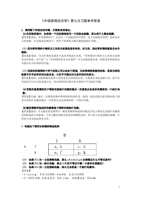
2. 考虑如下图所示的博弈得益矩阵(1)如果(T,L)为一占优策略均衡,那么a,b,c,d,e,f,,g,h必须满足什么不等式条件?(2)如果(T,L)为一纳什均衡,那么(1)中的不等式中哪一个条件必须满足?(3)如果(T,L)为一占优策略均衡,那么它必然是一个纳什均衡吗、【答案】(1)a>e, c>g T是占优策略;b>d, f>h L是占优策略(2)对纳什均衡, 如果A选T,则有a>=e;如果B选L,则b>=d。
尼科尔森微观经济学第11版笔记和课后习题答案
尼科尔森《微观经济理论——基本原理与扩展》(第11版)笔记和课后习题详解内容简介尼科尔森著作的《微观经济理论基本原理与扩展》(第11版)是世界上最受欢迎的中级微观经济学教材之一,被国内部分院校(如北京大学、中国人民大学、南京大学等)列为考研考博重要参考书目。
为了帮助学员更好地学习这本教材,我们精心编著了它的配套辅导用书(手机端及电脑端均可同步使用):1.尼科尔森《微观经济理论——基本原与扩展》(第11版)笔记和课后习题详解2.尼科尔森《微观经济理论—基本原理与扩展》(第11版)课后习题详解3.尼科尔森《微观经济理论基本原理与扩展》(第11版)配套题库【课后习题章节题库(含名校考研真题)+模拟试题】本书是尼科尔森《微观经济理论基本原理与扩展》(第11版)教材的配套电子书,严格按照教材内容编写,共分19章,主要包括以下内容(1)整理复习笔记,浓缩内容精华。
每章的复习笔记以尼科尔森《微观经济理论基本原理与扩展》(第11版)为主,并结合其他微观经济学经典教材对各章的重难点进行了整理,因此,本书的内容几乎浓缩了经典教材的知识精华。
(2)解析课后习题,提供详尽答案。
本书参考大量相关辅导资料对尼科尔森著作的《微观经济理论基本原理与扩展》(11版)的课后习题进行了详细的分析和解答,并对相关重要知识点进行了延伸和归纳。
目录第一篇引言第1章经济模型1.1 复习笔记1.2 课后习题详解第2章微观经济学中的数学工具2.1 复习笔记2.2 课后习题详解第二篇选择与需求第3章偏好与效用3.1 复习笔记3.2 课后习题详解第4章效用最大化与选择4.1 复习笔记4.2 课后习题详解第5章收入效应与替代效应5.1 复习笔记5.2 课后习题详解第6章商品间的需求关系6.1 复习笔记6.2. 课后习题详解第三篇不确定性与策略第7章不确定性7.1 复习笔记7.2 课后习题详解第8章博弈论8.1 复习笔记8.2 课后习题详解第四篇生产与供给第9章生产函数9.1 复习笔记9.2 课后习题详解第10章成本函数10.1 复习笔记10.2 课后习题详解第11章利润最大化11.1 复习笔记11.2 课后习题详解第五篇竞争性市场第12章竞争性价格决定的局部均衡模型12.1 复习笔记12.2 课后习题详解第13章一般均衡和福利13.1 复习笔记13.2 课后习题详解第六篇市场势力第14章垄断14.1 复习笔记14.2 课后习题详解第15章不完全竞争15.1 复习笔记15.2 课后习题详解第七篇要素市场定价第16章劳动力市场16.1 复习笔记16.2 课后习题详解第17章资本和时间17.1 复习笔记17.2 课后习题详解第八篇市场失灵第18章不对称信息18.1 复习笔记18.2 课后习题详解第19章外部性与公共品19.1 复习笔记19.2 课后习题详解第二章微观经济学中的数学工具1.已知U(x,y)=4x2+3y2。
中级微观经济学习题及答案
中级微观经济学习题及答案ANSWERS1 The Market1. Suppose that there were 25 people who had a reservation price of $500, and the 26th person had a reservation price of $200. What would the demand curve look like?1.1. It would be constant at $500 for 25 apartments and then drop to $200.2. In the above example, what would the equilibrium price be if there were 24 apartments to rent? What if there were 26 apartments to rent?What if there were 25 apartments to rent?1.2. In the ?rst case, $500, and in the second case, $200. In the third case, the equilibrium price would be any price between $200 and $500.3. If people have di?erent reservation prices, why does the market demand curve slope down?1.3. Because if we want to rent one more apartment, we have to o?er a lower price. The number of people who have reservation prices greater than p must always increase as p decreases.4. In the text we assumed that the condominium purchasers came from the inner-ring people—people who were already rentingapartments. What would happen to the price of inner-ring apartments if all of the condominium purchasers were outer-ring people—the people who were not currently renting apartments in the inner ring? 1.4. The price of apartments in the inner ring would go up since demand for apartments would not change but supply would decrease.5. Suppose now that the condominium purchasers were all inner-ring people, but that each condominium was constructed from two apartments. What would happen to the price of apartments?1.5. The price of apartments in the inner ring would rise.6. What do you suppose the e?ect of a tax would be on the number of apartments that would be built in the long run?1.6. A tax would undoubtedly reduce the number of apartments supplied in the long run.7. Suppose the demand curve is D(p) = 100?2p. What price would the monopolist set if he had 60 apartments? How many would he rent? What price would he set if he had 40 apartments? How many would he rent?1.7. He would set a price of 25 and rent 50 apartments. In the second case he would rent all 40 apartments at the maximum price the marketwould bear. This would be given by the solution to D(p) = 100?2p = 40, which is p? = 30.8. If our model of rent control allowed for unrestricted subletting, who would end up getting apartments in the inner circle? Would the outcome be Pareto e?cient?1.8. Everyone who had a reservation price higher than the equilibrium price in the competitive market, so that the ?nal outcome would be Pareto e?cient.(Of course in the long run there would probably be fewer new apartments built, which would lead to another kind of ine?ciency.)2 Budget Constraint1. Originally the consumer faces the budget line p1x1 + p2x2 = m. Then the price of good 1 doubles, the price of good 2 becomes 8 times larger, and income becomes 4 times larger. Write down an equation for the new budget line in terms of the original prices and income.2.1. The new budget line is given by 2p1x1 +8p2x2 =4m.2. What happens to the budget line if the price of good 2 increases, but the price of good 1 and income remain constant? 2.2. The vertical intercept (axis) decreases and the horizontalx2intercept (axis) stays the same. Thus the budget line becomes ?atter.x13. If the price of good 1 doubles and the price of good 2 triples, does the budget line become ?atter or steeper?2.3. Flatter. The slope is ?2/3.p1p24. What is the de?nition of a numeraire good?2.4. A good whose price has been set to 1; all other goods’ prices are measured relative to the numeraire good’s price.5. Suppose that the government puts a tax of 15 cents a gallon on gasoline and then later decides to put a subsidy on gasoline at a rate of 7 cents a gallon. What net tax is this combination equivalent to?2.5. A tax of 8 cents a gallon.6. Suppose that a budget equation is given by += m. Thep1x1p2x2 government decides to impose a lump-sum tax of u, a quantity tax on good 1 of t, and a quantity subsidy on good 2 of s. What is the formula for the new budget line?2.6. (+ t)+(?s)= m?u.p1x1p2x27. If the income of the consumer increases and one of the prices decreases at the same time, will the consumer necessarily be at leastas well-o??2.7. Yes, since all of the bundles the consumer could a?ord before are a?ordable at the new prices and income.3 Preferences1. If we observe a consumer choosing (,) when (,) is availablex1x2y1y2one time, are we justi?ed in concluding that (,)>(,)?x1x2y1y23.1. No. It might be that the consumer was indi?erent between the two bundles. All we are justi?ed in concluding is that (,)> (,).x1x2y1y22. Consider a group of people A, B, C and the relation “at least as tall as,” as in “A is at least as tall as B.” Is this relation transitive? Is it complete?3.2. Yes to both.3. Take the same group of people and consider the relation “strictly taller than.” Is this relation transitive? Is it re?exive? Is it complete? 3.3. It is transitive, but it is not complete—two people might be the same height. It is not re?exive since it is false that a person is strictly taller than himself.4. A college football coach says that given any two linemen A and B, he always prefers the one who is bigger and faster. Is this preferencerelation transitive? Is it complete?3.4. It is transitive, but not complete. What if A were bigger but slower than B? Which one would he prefer?5. Can an indi?erence curve cross itself? For example, could Figure 3.2 depict a single indi?erence curve?3.5. Yes. An indi?erence curve can cross itself, it just can’t cross another distinct indi?erence curve.6. Could Figure 3.2 be a single indi?erence curve if preferences are monotonic?3.6. No, because there are bundles on the indi?erence curve that have strictly more of both goods than other bundles on the (alleged) indi?erence curve.7. If both pepperoni and anchovies are bads, will the indi?erence curve have a positive or a negative slope?3.7. A negative slope. If you give the consumer more anchovies, you’ve made him worse o?, so you have to take away some pepperoni to get him back on his indi?erence curve. In this case the direction of increasing utility is toward the origin.8. Explain why convex preferences means that “averages are preferred to extremes.”3.8. Because the consumer weakly prefers the weighted average of two bundles to either bundle.9. What is your marginal rate of substitution of $1 bills for $5 bills?3.9. If you give up one $5 bill, how many $1 bills do you need to compensate you? Five $1 bills will do nicely. Hence the answer is ?5 or?1/5, depending on which good you put on the horizontal axis.10. If good 1 is a “neutral,” what is its marginal rate of substitution for good 2?3.10. Zero—if you take away some of good 1, the consumer needs zero units of good 2 to compensate him for his loss. ANSWERS A1311. Think of some other goods for which your preferences might be concave.3.11. Anchovies and peanut butter, scotch and Kool Aid, and other similar repulsive combinations.4 Utility1. The text said that raising a number to an odd power was amonotonic transformation. What about raising a number to an even power? Is this a monotonic transformation? (Hint: consider the case f(u)=u^2.)4.1. The function f(u)=u^2 is a monotonic transformation for positive u, but not for negative u.2. Which of the following are monotonic transformations?(1) u =2 v?13;(2) u = ?1/v^2;(3)u =1/v^2; (4)u = ln v; (5)u = ?e^?v; (6)u = v^2; (7) u = v^2 for v>0; (8) u = v^2 for v<0.4.2. (1) Yes. (2) No (works for v positive). (3) No (works for v negative).(4) Yes (only de?ned for v positive). (5) Yes. (6) No. (7) Yes. (8) No.3. We claimed in the text that if preferences were monotonic, then a diagonal line through the origin would intersect each indi?erence curve exactly once. Can you prove this rigorously? (Hint: what would happen if it intersected some indi?erence curve twice?)4.3. Suppose that the diagonal intersected a given indi?erence curve at two points, say (x,x) and (y,y). Then either x>y or y>x, which means that one of the bundles has more of both goods. But if preferences are monotonic, then one of the bundles would have to be preferred to the other.4. What kind of preferences are represented by a utility function of thex1+x2form u(x1,x2)=? What about the utility function v(x1,x2)= 13x1 + 13x2?4.4. Both represent perfect substitutes.5. What kind of preferences are represented by a utility function of thex2x2 form u(x1,x2)=x1 +? Is the utility function v(x1,x2)=x2 1 +2x1+x2 a monotonic transformation of u(x1,x2)?4.5. Quasilinear preferences. Yes.x1x26. Consider the utility function u(x1,x2)=. What kind of pref- erences does it represent? Is the function v(,)= ax1x2x12x22 monotonic transformation of u(,)? Is the function w(,) =x1x2x1x2x12a monotonic transformation of u(,)?x22x1x24.6. The utility function represents Cobb-Douglas preferences. No. Yes.7. Can you explain why taking a monotonic transformation of a utility function doesn’t change the marginal rate of substitution?4.7. Because the MRS is measured along an indi?erence curve, and utility remains constant along an indi?erence curve.5 Choice1. If two goods are perfect substitutes, what is the demand function forgood 2?5.1.=0 when>, = m/when <, and anything betweenx2 p2p1x2p2p2p10 and m/p2 when = .p1p22. Suppose that indi?erence curves are described by straight lines witha slope of ?b. Given arbitrary prices and money income p1, p2, and m, what will the consumer’s optimal choices look like?5.2. The optimal choices will be x1 = m/p1 and x2 = 0 ifp1/p2 b, and any amount on the budget line if p1/p2 = b.3. Suppose that a consumer always consumes 2 spoons of sugar with each cup of co?ee. If the price of sugar is p1 per spoonful and the price of co?ee is p2 per cup and the consumer has m dollars to spend on co?ee and sugar, how much will he or she want to purchase?5.3. Let z be the number of cups of co?ee the consumer buys. Then we know that 2z is the number of teaspoons of sugar he or she buys. We must satisfy the budget constraint2z + z = m.p1p2Solving for z we havez =m2p1+ p2.4. Suppose that you have highly nonconvex preferences for ice cream and olives, like those given in the text, and that you face prices p1, p2 and have m dollars to spend. List the choices for the optimal consumption bundles.5.4. We know that you’ll either consume all ice cream or all olives. Thus the two choices for the optimal consumption bundles will be x1 = m/,p1 x2 = 0, or x1 = 0, x2 = m/.p25. If a consumer has a utility function u(x1,x2)=x1x4 2, what fraction of her income will she spend on good 2?5.5. This is a Cobb-Douglas utility function, so she will spend 4/(1 + 4) = 4/5 of her income on good 2.6. For what kind of preferences will the consumer be just as well-o?facing a quantity tax as an income tax?5.6. For kinked preferences, such as perfect complements, where the change in price doesn’t induce any change in demand.6 Demand1. If the consumer is consuming exactly two goods, and she is always spending all of her money, can both of them be inferior goods?6.1. No. If her income increases, and she spends it all, she must be purchasing more of at least one good.2. Show that perfect substitutes are an example of homotheticpreferences.6.2. The utility function for perfect substitutes is u(,)=+ .x1 x2 x1 x2Thus if u(,) >u (,), we have + >+ . It follows x1 x2 y1 y2 x1 x2 y1y2that t+ t> t+ t, so that u(t,t) >u (t, t).x1 x2 y1y2 x1 x2 y1y23. Show that Cobb-Douglas preferences are homothetic preferences.6.3. The Cobb-Douglas utility function has the property that u(t,t)=x1 x2= 2 = t 2 = t*u(x1,). ( t x1)a( t x2)1?a t a t1?a x1a x21?a x1a x21?a x2Thus if u(,) >u (,), we know that u(t,t) >u (t,), so x1 x2 y1 y2 x1 x2 y1t y2that Cobb-Douglas preferences are indeed homothetic.4. The income o?er curve is to the Engel curve as the price o?er curveis to ...?6.4. The demand curve.5. If the preferences are concave will the consumer ever consume bothof the goods together?6.5. No. Concave preferences can only give rise to optimal consumptionbundles that involve zero consumption of one of the goods.。
尼科尔森《微观经济理论—基本原理与扩展》(第9版)课后习题详解
尼科尔森《微观经济理论—基本原理与扩展》(第9版)课后习题详解第1篇引言第1章经济模型本章没有课后习题。
本章是全书的一个导言,主要要求读者对微观经济模型有一个整体了解,然后在以后各章的学习中逐渐深化认识。
第2章最优化的数学表达1.假设。
(1)计算偏导数,。
(2)求出上述偏导数在,处的值。
(3)写出的全微分。
(4)计算时的值——这意味着当保持不变时,与的替代关系是什么?(5)验证:当,时,。
(6)当保持时,且偏离,时,和的变化率是多少?(7)更一般的,当时,该函数的等高线是什么形状的?该等高线的斜率是多少?解:(1)对于函数,其关于和的偏导数分别为:,(2)当,时,(1)中的偏微分值分别为:,(3)的全微分为:(4)当时,由(3)可知:,从而可以解得:。
(5)将,代入的表达式,可得:。
(6)由(4)可得,在,处,当保持不变,即时,有:(7)当时,该函数变为:,因而该等高线是一个中心在原点的椭圆。
由(4)可知,该等高线在(,)处的斜率为:。
2.假定公司的总收益取决于产量(),即总收益函数为:;总成本也取决于产量():。
(1)为了使利润()最大化,公司的产量水平应该是多少?利润是多少?(2)验证:在(1)中的产量水平下,利润最大化的二阶条件是满足的。
(3)此处求得的解满足“边际收益等于边际成本”的准则吗?请加以解释。
解:(1)由已知可得该公司的利润函数为:利润最大化的一阶条件为:从而可以解得利润最大化的产量为:;相应的最大化的利润为:。
(2)在处,利润最大化的二阶条件为:,因而满足利润最大化的二阶条件。
(3)在处,边际收益为:;边际成本为:;因而有,即“边际收益等于边际成本”准则满足。
3.假设。
如果与的和是1,求此约束下的最大值。
利用代入消元法和拉格朗日乘数法两种方法来求解此问题。
解:(1)代入消元法由可得:,将其代入可得:。
从而有:,可以解得:。
从而,。
(2)拉格朗日乘数法的最大值问题为:构造拉格朗日函数为:一阶条件为:从而可以解得:,因而有:。
北大ccer考研历年试题含答案微观题目

一、简答题(共15分)1、(5分)如果生产函数是不变规模报酬的生产函数,企业长期平均成本曲线是否一定是下降的?为什么?2、(5分)有人说,在出现了污染这种外部性的条件下,没有政府的干预,就不可能达到帕累托效率条件。
这种说法是否正确?为什么?3、(5分)即使不存在逆选择问题,财产保险公司通常也不开办旨在为投保人提供全额赔偿的保险。
为什么?二、计算题(共35分)1、(8分)假定某垄断厂商可以在两个分隔的市场上实行价格歧视。
两个分隔的市场上,该厂商所面临的需求曲线分别表示如下:市场1:q1=a1-b1p1; 市场2:q2=a2-b2p2假定厂商的边际成本与平均成本为常数c。
请证明,垄断者无论是实行价格歧视(在两个市场上收取不同的价格),还是不实行价格歧视(在两个市场上收取相同的价格),这两种定价策略下的产出水平都是相同的。
2、(5分)如果某种股票的β值是1.2;整个股票市场的年盈利率是20%;无风险资产的年盈利率是10%。
按照资本资产定价模型,该种资产的期望年盈利率是多高?如果该股票一年后的期望值是20元,该股票的现在市场价格应该是多少?3、(8分)假定某种产品市场上有两个寡头,两寡头生产相同产品,进行产量竞争。
两个寡头的行为遵从斯泰克伯格模型。
寡头1为领导者,寡头2为跟从者。
产品的市场价格为:p=200-(q1+q2),其中,q1、q2分别为寡头1与寡头2的产量。
如果两个寡头边际成本与平均成本相同,并保持不变,即AC=MC=60。
求两个寡头利润最大化的产量。
4、(6分)在竞赛者1与竞赛者2所进行的二人竞赛中,竞赛者1可以采取上或下两种策略,竞赛者2可以采取左或右两种策略。
两竞赛者的支付矩阵如下:竞赛者2竞赛者1左右上(9,14) (5,2)下(7,-10) (17,-15)问,竞赛者1是否存在优势策略,为什么?5、(8分)对某钢铁公司某种钢X的需求受到该种钢的价格Px、钢的替代品铝的价格Py,以及收入M的影响。
中级微观课后思考题答案

中级微观课后思考题答案1名词解释1、需求的价格弹性:一种商品的需求量对它自身价格变化的反映灵敏度。
2、经济学:经济学是研究人和社会如何进行选择,来使用可以有其他用途的稀缺的资源,以便生产各种商品,并在现在或者将来把商品分配给社会各种成员或集团以供消费者之用的科学。
3、消费者剩余:需求曲线和价格曲线之间的面积,衡量消费者在市场交易中得到的福利(净好处)。
愿意支付的价格与实际支付价格之差。
5、实证经济学:客观描述和分析经济现象和规律。
(像经济学家一样思考)6、需求定理:在其他条件不变的情况下,商品的需求量和商品自身的价格呈反向变动的关系。
即价格越低、需求量越大。
7、市场均衡:当市场上需求和供给双方的力量势均力敌,从而市场上产品价格和产品量处于相对稳定的状态。
均衡,意味着在某一价格下全体消费者愿意且能够购买的量刚好等于全体厂商愿意且能够提供的量,是市场出清状态。
8、价格上限简答题:1、经济学的基本问题是什么?三大问题生产什么和生产多少?如何生产?为谁生产?(分配)解决方法计划经济(指令经济)市场经济(效率)混合经济(市场为主,政府为辅)2、政府的基本职能是什么?弥补市场经济的缺陷1、促进效率(1)不完全竞争市场(垄断)。
(2)外部性(3)公共品(4)不完全信息,不对称信息2、促进经济公平3、保证宏观经济的稳定和增长(财政政策,货币政策)3、什么是完全竞争市场?市场上有大量的买者和卖者,以至于每个人对市场价格的影响的微乎其微的市场结构。
4、影响需求的因素有那些?商品自身的价格互补品相关商品的价格替代品正常品消费者的收入低档品消费者的偏好消费者的价格和收入预期5、什么是供给的变动?什么是供给量的变动?6、什么是税收归宿?7、简述弹性和总收益的关系。
论述题:1、竞争性市场是如何实现均衡的?为什么说竞争性的市场均衡是有效率的?2、如果政府对农产品实施保护价格,请分析保护价格对经济的影响。
支持价格是指为了避免市场自发形成的均衡价格太低而损害生产者的利益,政府对产品制定高于均衡价格的最低价格。
尼科尔森《微观经济理论-基本原理与扩展》(第9版)课后习题详解(第4章 效用最大化与选择)
尼科尔森《微观经济理论-基本原理与扩展》(第9版)第4章 效用最大化与选择课后习题详解跨考网独家整理最全经济学考研真题,经济学考研课后习题解析资料库,您可以在这里查阅历年经济学考研真题,经济学考研课后习题,经济学考研参考书等内容,更有跨考考研历年辅导的经济学学哥学姐的经济学考研经验,从前辈中获得的经验对初学者来说是宝贵的财富,这或许能帮你少走弯路,躲开一些陷阱。
以下内容为跨考网独家整理,如您还需更多考研资料,可选择经济学一对一在线咨询进行咨询。
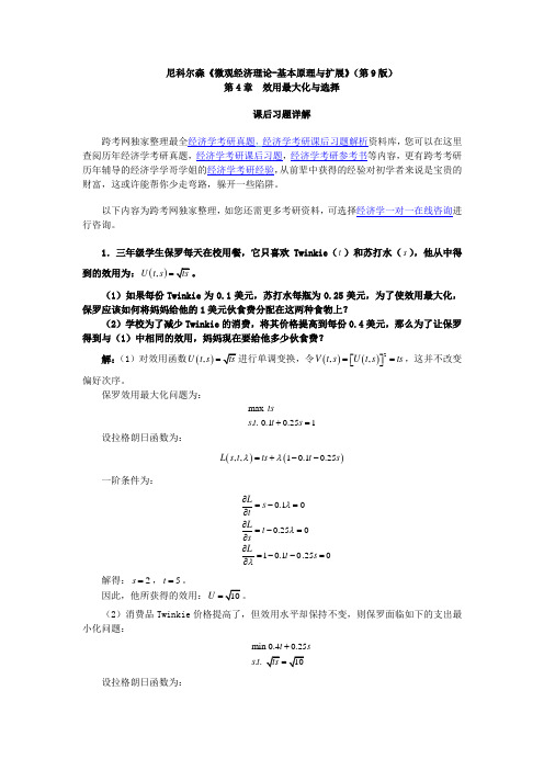
1.三年级学生保罗每天在校用餐,它只喜欢Twinkie (t )和苏打水(s ),他从中得到的效用为:(),U t s ts =。
(1)如果每份Twinkie 为0.1美元,苏打水每瓶为0.25美元,为了使效用最大化,保罗应该如何将妈妈给他的1美元伙食费分配在这两种食物上?(2)学校为了减少Twinkie 的消费,将其价格提高到每份0.4美元,那么为了让保罗得到与(1)中相同的效用,妈妈现在要给他多少伙食费?解:(1)对效用函数(),U t s ts =进行单调变换,令()()2,,V t s U t s ts ==⎡⎤⎣⎦,这并不改变偏好次序。
保罗效用最大化问题为:max .. 0.10.251tss t t s +=设拉格朗日函数为:()(),,10.10.25L s t ts t s λλ=+--一阶条件为:0.100.25010.10.250Ls t Lt s Lt s λλλ∂=-=∂∂=-=∂∂=--=∂ 解得:2s =,5t =。
因此,他所获得的效用:10U =(2)消费品Twinkie 价格提高了,但效用水平却保持不变,则保罗面临如下的支出最小化问题:min 0.40.25..10t s s tts +=设拉格朗日函数为:()(),,0.40.2510L s t t s ts λλ=++-一阶条件为:0.40Ls tλ∂=-=∂ (1) 0.25Lt sλ∂=-=0∂ (2) 100Lts λ∂=-=∂ (3) 由上述三式解得 2.5t =,4s =,则最小支出为:10.4 2.50.2542m =⨯+⨯=,所以妈妈现在要给他2美元伙食费使他的效用水平保持不变。
中级微观经济学课后习题

中级微观经济学课后习题(总18页)--本页仅作为文档封面,使用时请直接删除即可----内页可以根据需求调整合适字体及大小--第2章预算约束1.消费者的最初预算线是p1x1+p2x2=m。
接着,商品1的价格提高了1倍,商品2的价格提高了7倍,收入增加了3倍。
根据原先的价格和收入写出新的预算线的方程。
2.如果商品2的价格上涨了,而商品1的价格和收入保持不变,预算线会有什么变化3.如果商品1的价格上涨了1倍,商品2的价格上涨了2倍,预算线是变得平缓了还是变得陡峭了4.计价物的定义是什么5.假设政府起初对每加仑汽油征税15美分,后来,又决定对每加仑汽油补贴7美分。
这两种方法混合运用后的税收是多少6.假设预算方程是p1x1+p2x2=m。
如果政府决定征收u单位的总额税、对商品1征收t单位的从量税,以及对商品2进行从量补贴s,新预算线的公式是什么7.如果消费者的收入增加了,同时有一种商品的价格下降了,那么消费者的境况会与原来一样好吗第3章偏好1.如果我们有一次看到,某消费者在(y1,y2)可以同时得到的情况下选择了(x1,x2),那么,(x1,x2)>(y1,y2)的结论正确吗2.假设有三个人A,B和C,身高关系为“至少和…一样高”,比如“A至少和B 一样高”。
这样的关系是传递的吗是完备的吗3.假设有三个人A,B和C,身高关系为“严格高于”。
这样的关系是传递的吗是反身的吗是完备的吗4.某大学橄榄球教练说,任意给定两个前锋比如A和B,他永远偏好身材更高大和速度更快的那个。
他的这种偏好关系是传递的吗是完备的吗5.某条无差异曲线能否与自身相交例如,图能否是一条无差异曲线而不是两条6.如果偏好是单调的,能否把图看成一条无差异曲线而不是两条7.如果辣香肠和凤尾鱼都是厌恶品,那么无差异曲线的斜率为正还是负8.解释为什么凸偏好意味着“平均束好于端点束”。
11.举例说明你的偏好在什么样的情形下为凹的。
第4章效用1.课文中说,将某数字变为它的奇次幂是一种单调变换。
尼克尔森微观经济学课后答案
尼克尔森微观经济学课后答案CHAPTER 2THE MATHEMATICS OF OPTIMIZATIONThe problems in this chapter are primarily mathematical. They are intended to give students some practice with taking derivatives and using the Lagrangian techniques, but the problems in themselves offer few economic insights. Consequently, no commentary is provided. All of the problems are relatively simple and instructors might choose from among them on the basis of how they wish to approach the teaching of the optimization methods in class.Solutions2.1 22(,)43=+U x y x y a.86 U U = x , = y x y b.8, 12 c. 86??=?? U U dU dx + dy = x dx + y dy x y d. for 0 8 6 0=+=dy dU x dx y dy dx 8463--dy x x = = dx y ye.1,2413416===?+?=x y U f.4(1)2/33(2)-==-dy dx g. U = 16 contour line is an ellipse centered at the origin.With equation 224316+=x y , slope of the line at (x, y ) is43=-dy x dx y.2.2 a. Profits are given by 2240100π=-=-+-R C q q*44010π=-+=d q q dq2*2(1040(10)100100)π=-+-= b. 224π=-d dq so profits are maximized c. 702==-dR MR q dq 230==+dC MCq dq so q * = 10 obeys MR = MC = 50.2.3 Substitution:21 so =-==-y x f xy x x120?=-=?f x x0.50.5,0.25x =, y = f =Note: 20''=-Lagrangian Method: ?1)λ=+--xy x y£λ?-? = y = 0x£λ?-? = x = 0yso, x = y.using the constraint gives 0.5,0.25===x y xy2.4 Setting up the Lagrangian: ?0.25)λ=++-x y xy .£1£1λλ?=-??=-?y x x ySo, x = y . Using the constraint gives 20.25,0.5====xy x x y .2.5 a. 2()0.540=-+f t gt t*40400,=-+==df g t t dt g . b.Substituting for t*, *2()0.5(40)40(40)800=-+=f t g g g g . *2()800?=-?f t g g. c. 2*1()2=-f t g depends on g because t * depends on g . so*222408000.5()0.5()?-=-=-=?f t g g g . d. 8003225,80032.124.92==, a reduction of .08. Notice that 22800800320.8-=≈-g so a 0.1 increase in g could bepredicted to reduce height by 0.08 from the envelope theorem.2.6 a. This is the volume of a rectangular solid made from a piece ofmetal which is x by 3x with the defined corner squares removed. b. 22316120?=-+=?V x xt t t. Applying the quadratic formula to this expressionyields1610.60.225, 1.1124±===x x t x x . Todetermine true maximum must look at second derivative --221624?=-+?V x t twhich is negative only for the first solution.c. If 33330.225,0.67.04.050.68=≈-+≈t x V x x x x so V increaseswithout limit.d. This would require a solution using the Lagrangian method. Theoptimal solution requires solving three non-linear simultaneousequations —a task not undertaken here. But it seems clear thatthe solution would involve a different relationship between tand x than in parts a-c.2.7 a. Set up Lagrangian 1212?ln ()λ=++--x x k x x yields the first order conditions: 12212£10?0£0λλλ?=-=??=-=??=--=?x x x k x xHence, 2215 or 5λ===x x . With k = 10, optimal solution is 12 5.==x xb. With k = 4, solving the first order conditions yields215, 1.==-x xc. Optimal solution is 120,4,5ln 4.===x x y Any positive value forx 1 reduces y.d. If k = 20, optimal solution is 1215, 5.==x x Because x 2provides a diminishing marginal increment to y whereas x 1 doesnot, all optimal solutions require that, once x 2 reaches 5, anyextra amounts be devoted entirely to x 1.2.8 The proof is most easily accomplished through the use of the matrixalgebra of quadratic forms. See, for example, Mas Colell et al.,pp. 937–939. Intuitively, because concave functions lie belowany tangent plane, their level curves must also be convex. Butthe converse is not true. Quasi-concave functions may exhibit“increasing returns to scale”; even though their level curvesare convex, they may rise above the tangent plane when allvariables are increased together.2.9 a.11210.βαα-=> f x x 11220βαβ-=> f .x x21111(1)0.βααα-=-< f x x21222(1)0.βαββ-=-< f x x111212210.βααβ--==> f f x xClearly, all the terms in Equation 2.114 are negative. b.If 12βα==y c x x /1/21αββ-= x c x since α, β > 0, x 2 is a convex function of x 1 .c.Using equation 2.98, 222222222221122111222(1)()(1)ββααααβββα-----=--- f f f x x x x= 222212(1)βααββα---- x x which is negative for α + β > 1.2.10 a.Since 0,0'''>Because 1122,0y is quasi-concave as is γy . But γy is not concave for γ > 1. All of these results can be shown by applying the various definitions to the partial derivatives of y .CHAPTER 3PREFERENCES AND UTILITYThese problems provide some practice in examining utility functions by looking at indifference curve maps. The primary focus is on illustrating the notion of a diminishing MRS in various contexts. The concepts of the budget constraint and utility maximization are not used until the next chapter.Comments on Problems3.1 This problem requires students to graph indifference curves for a varietyof functions, some of which do not exhibit a diminishing MRS.3.2 Introduces the formal definition of quasi-concavity (from Chapter 2) to beapplied to the functions in Problem 3.1.3.3 This problem shows that diminishing marginal utility is not required toobtain a diminishing MRS. All of the functions are monotonic transformations of one another, so this problem illustrates that diminishing MRS is preserved by monotonic transformations, but diminishing marginal utility is not.3.4 This problem focuses on whether some simple utility functions exhibit convexindifference curves.3.5 This problem is an exploration of the fixed-proportions utility function.The problem also shows how such problems can be treated as a composite commodity.3.6 In this problem students are asked to provide a formal, utility-basedexplanation for a variety of advertising slogans. The purpose is to get students to think mathematically about everyday expressions.3.7 This problem shows how initial endowments can be incorporated into utilitytheory.3.8This problem offers a further exploration of the Cobb-Douglas function.Part c provides an introduction to the linear expenditure system. This application is treated in more detail in the Extensions to Chapter 4.。
尼库尔森《微观经济学》课后答案ch18
CHAPTER 18UNCERTAINTY AND RISK AVERSIONMost of the problems in this chapter focus on illustrating the concept of risk aversion. That is, they assume that individuals have concave utility of wealth functions and therefore dislike variance in their wealth. A difficulty with this focus is that, in general, students will not have been exposed to the statistical concepts of a random variable and its moments (mean, variance, etc.). Most of the problems here do not assume such knowledge, but the Extensions do show how understanding statistical concepts is crucial to reading applications on this topic.Comments on Problems18.1 Reverses the risk-aversion logic to show that observed behavior can be used to placebounds on subjective probability estimates.18.2 This problem provides a graphical introduction to the idea of risk-taking behavior. TheFriedman-Savage analysis of coexisting insurance purchases and gambling could bepresented here.18.3 This is a nice, homey problem about diversification. Can be done graphically althoughinstructors could introduce variances into the problem if desired.18.4 A graphical introduction to the economics of health insurance that examines cost-sharingprovisions. The problem is extended in Problem 19.3.18.5 Problem provides some simple numerical calculations involving risk aversion andinsurance. The problem is extended to consider moral hazard in Problem 19.2.18.6 This is a rather difficult problem as written. It can be simplified by using a particularutility function (e.g., U(W) = ln W). With the logarithmic utility function, one cannot use the Taylor approximation until after differentiation, however. If the approximation isapplied before differentiation, concavity (and risk aversion) is lost. This problem can,with specific numbers, also be done graphically, if desired. The notion that fines aremore effective can be contrasted with the criminologist’s view that apprehension of law-breakers is more effective and some shortcomings of the economic argument (i.e., nodisutility from apprehension) might be mentioned.18.7 This is another illustration of diversification. Also shows how insurance provisions canaffect diversification.18.8 This problem stresses the close connection between the relative risk-aversion parameterand the elasticity of substitution. It is a good problem for building an intuitive9798 Solutions Manualunderstanding of risk-aversion in the state preference model. Part d uses the CRRAutility function to examine the “equity-premium puzzle.”18.9 Provides an illustration of investment theory in the state preference framework.18.10 A continuation of Problem 18.9 that analyzes the effect of taxation on risk-takingbehavior.Solutions18.1 p must be large enough so that expected utility with bet is greater than or equal to thatwithout bet: p ln(1,100,000) + (1 –p)ln(900,000) > ln(1,000,000)13.9108p +13.7102(1 –p) > 13.8155, .2006p > .1053 p > .52518.2This would be limited by the individual’s resources: he or she could run out of wealth since unfair bets are continually being accepted.18.3 a.Strategy One Outcome Probability12 Eggs .50 Eggs .5Expected Value = .5∙12 + .5∙0 = 6Strategy Two Outcome Probability12 Eggs .256 Eggs .50 Eggs .25Expected Value = .25 ∙12 + .5 ∙ 6 + .25∙ 0= 3 + 3 = 6Chapter 18/Uncertainty and Risk Aversion 99b.18.4 a. E(L) = .50(10,000) = $5,000, soWealth = $15,000 with insurance, $10,000 or $20,000 without.b. Cost of policy is .5(5000) = 2500. Hence, wealth is 17,500 with no illness, 12,500with the illness.18.5 a. E(U) = .75ln(10,000) + .25ln(9,000) = 9.1840b. E(U) = ln(9,750) = 9.1850 Insurance is preferable.c. ln(10,000 – p ) = 9.184010,000 – p = e 9.1840 = 9,740p = 26018.6 Expected utility = pU(W – f) + (1 – p)U(W). ,[()()]/U p U pU W f U W p U e p U∂=⋅=--⋅∂,()/U f U fp U W f f U e f U∂'=⋅=-⋅-⋅∂100 Solutions Manual,,()()1()U p U fU W f U W e f U W f e --=<'-- by Taylor expansion,So, fine is more effective.If U (W ) = ln W then Expected Utility = p ln (W – f ) + (1 – p ) ln W .,/[ln ()ln ]U pp p f WW f W e U U -=--⋅≈ ,/()/()U ff p f W f p U W f e U U--=--⋅= ,,1U p U fW fe W e -=<18.7 a. U (wheat) = .5 ln(28,000) + .5 ln(10,000) = 9.7251 U (corn) = .5 ln(19,000) + .5 ln(15,000) = 9.7340 Plant corn. b. With half in eachY NR = 23,500Y R = 12,500U = .5 ln(23,500) + .5 ln(12,500) = 9.7491Should plant a mixed crop. Diversification yields an increased variance relative to corn only, but takes advantage of wheat’s high yield.c. Let α = percent in wheat. U = .5 ln[ (28,000) + (1 – α )(19,000)] + .5 ln[α (10,000) + (1 – α )(15,000)] = .5 ln(19,000 + 9,000α) + .5 ln(15,000 – 5,000α)45002500019,0009,00015,0005,000dU d ααα=-=+- 45(150 – 50α) = 25(190 + 90α) α = .444 U = .5 ln(22,996) + .5 ln(12,780) = 9.7494. This is a slight improvement over the 50-50 mix. d. If the farmer plants only wheat,Y NR = 24,000Y R = 14,000U = .5 ln(24,000) + .5 ln(14,000) = 9.8163so availability of this insurance will cause the farmer to forego diversification.Chapter 18/Uncertainty and Risk Aversion 10118.8 a. A high value for 1 – R implies a low elasticity of substitution between states of theworld. A very risk-averse individual is not willing to make trades away from the certainty line except at very favorable terms.b. R = 1 implies the individual is risk-neutral. The elasticity of substitution between wealth in various states of the world is infinite. Indifference curves are linear with slopes of –1. If R =-∞, then the individual has an infinite relative risk-aversion parameter. His or her indifference curves are L-shaped implying an unwillingness to trade away from the certainty line at any price.c. A rise in b p rotates the budget constraint counterclockwise about the W g intercept. Both substitution and income effects cause W b to fall. There is a substitution effect favoring an increase in W g but an income effect favoring a decline. The substitution effect will be larger the larger is the elasticity of substitution between states (the smaller is the degree of risk-aversion).d. i. Need to find R that solves the equation:R R R W W W )955.0(5.0)055.1(5.0)(000+=This yields an approximate value for R of –3, a number consistent with some empirical studies.ii. A 2 percent premium roughly compensates for a ±10 percent gamble. That is:303030)12.1()92(.)(---+≈W W W .The “puzzle” is that the premium rate of return provided by equities seems to be much higher than this.18.9 a. See graph.Risk free option is R , risk option is R '. b. Locus RR' represents mixed portfolios.c. Risk-aversion as represented by curvature of indifference curves will determine equilibrium in RR' (say E ).102 Solutions Manuald. With constant relative risk-aversion, indifference curve map is homothetic so locus ofoptimal points for changing values of W will be along OE.18.10 a. Because of homothetic indifference map, a wealth tax will cause movement along OE(see Problem 18.9).b. A tax on risk-free assets shifts R inward to Rt (see figure below). A flatter RR t'provides incentives to increase proportion of wealth held in risk assets, especially for individuals with lower relative risk-aversion parameters. Still, as the “note” implies, it is important to differentiate between the after tax optimum and the before taxchoices that yield that optimum. In the figure below, the no-tax choice is E on RR'.* EW represents the locus of points along which the fraction of wealth held in risky assets is constant. With the constraint RR t' choices are even more likely to be to the right of EW* implying greater investment in risky assets.c. With a tax on both assets, budget constraint shifts in a parallel way to RR tt'. Even in this case (with constant relative risk aversion) the proportion of wealth devoted to risky assets will increase since the new optimum will lie along OE whereas a constant proportion of risky asset holding lies along EW O.103。
北京大学中心中级微观经济学习题和答案 11

− 4cF 2
) ⇒ cF
= 0,U
= 80
显然,前一种生产方式最终的效用最大.故 social planner 会按照前一种生产方式安排生 产,并将最后的产出分配给 Robison 或者 Friday 中的一个.
如果,F 只生产 FF ,则
U
则最后的效用函数可以表示为:
=
16 (
− cR 2
)cR
maxU ⇒ cR = 13, FR = 3 / 2, FF = 5.,U = 169 / 2
如果,C 只生产 cR
光华人 向上的精神
U
则最后的效用函数可以表示为:
=
(16
+
cF
)(10
•ω
4 A
2.设商品 2 的价格为 1,商品 1 的价格为 p.
A : max
x1A
⋅
x
2 A
,
st,
px1A
+
x
2 A
=
3p
+
2
L
=
x1A
⋅
x
2 A
+
λ(3 p
+
2
−
px1A
−
x
2 A
)
⇒
x1A
=
3p + 2p
2
,
x
2 A
=
3p + 2
2
B : max x1B
⋅
x
2 B
,
st,
px1B
+
x
2 B
=
况.
讨论: ① 当 1/2<p<2 时
有 cR' =16, FF' =5
尼科尔森《微观经济理论——基本原理与扩展》课后习题详解-要素市场定价【圣才出品】

第6篇要素市场定价第16章劳动市场1.假定一年中有8000小时(实际上有8760小时),某人的潜在市场工资为5美元/小时。
(1)此人的最高临界收入是多少?如果他(或她)选择将75%的收入用于休闲,则他将工作多少小时?(2)假定此人的一个富有的叔叔去世了,留给了他(或她)一笔每年4000美元的收入。
如果他(或她)继续将其最高临界收入的75%用于休闲,则他将工作多少小时?(3)如果市场工资从5美元/小时提高至10美元/小时,则你对(2)的答案有何变化?(4)画出(2)和(3)所揭示的个人劳动供给曲线。
解:(1)此人全部收入为:8000540000⨯=(美元/年);其中,用于休闲的支出为:0.754000030000⨯=(美元/年);因而此人每年用于闲暇的时间为:30000/56000=(小时);用于工作的时间为:800060002000-=(小时)。
(2)在此人得到遗产后,他的全收入为:40000400044000+=(美元/年);其中,用于休闲的支出为:0.754400033000⨯=(美元/年);因而此人每年用于闲暇的时间为:33000/56600=(小时);用于工作的时间为:800066001400-=(小时)。
(3)如果市场工资提高后,他的全收入为:800010400084000⨯+=(美元/年);其中,用于休闲的支出为:0.758400063000⨯=(美元/年);因而此人每年用于闲暇的时间为:63000/106300=(小时);用于工作的时间为:800063001700-=(小时)。
(4)此人的劳动供给曲线如图16-1所示,当w 上升时,劳动供给趋近于2000小时。
图16-1个人劳动供给曲线2.假定某人对消费和闲暇的效用函数采取柯布-道格拉斯形式:()1,U c h c h αα-=。
支出最小化问题为:()()1min 24..,c w h s t U c h c h Uαα---==(1)利用此方法来得出支出函数。
尼克尔森微观经济学课后答案

CHAPTER 2THE MATHEMATICS OF OPTIMIZATIONThe problems in this chapter are primarily mathematical. They are intended to give students some practice with taking derivatives and using the Lagrangian techniques, but the problems in themselves offer few economic insights. Consequently, no commentary is provided. All of the problems are relatively simple and instructors might choose from among them on the basis of how they wish to approach the teaching of the optimization methods in class.Solutions2.122(,)43=+U x y x ya. 86∂∂∂∂ U U= x , = y x yb. 8, 12c. 86∂∂=∂∂ U UdU dx + dy = x dx + y dy x yd.for 0 8 6 0=+=dydU x dx y dy dx8463--dy x x = = dx y ye. 1,2413416===⋅+⋅=x y Uf. 4(1)2/33(2)-==-dy dx g.U = 16 contour line is an ellipse centered at the origin. With equation 224316+=x y , slope of the line at (x, y ) is43=-dy x dx y.2.2 a. Profits are given by 2240100π=-=-+-R C q q*44010π=-+=d q q dq2*2(1040(10)100100)π=-+-=b.224π=-d dqso profits are maximized c. 702==-dRMRq dq230==+dCMCq dqso q * = 10 obeys MR = MC = 50.2.3Substitution:21 so =-==-y x f xy x x120∂=-=∂fx x0.50.5,0.25x =, y = f =Note: 20''=-<f . This is a local and global maximum. Lagrangian Method: ?1)λ=+--xy x y £λ∂-∂= y = 0x£λ∂-∂= x = 0yso, x = y.using the constraint gives 0.5,0.25===x y xy 2.4Setting up the Lagrangian: ?0.25)λ=++-x y xy .£1£1λλ∂=-∂∂=-∂y xx ySo, x = y . Using the constraint gives 20.25,0.5====xy x x y .2.5a. 2()0.540=-+f t gt t *40400,=-+==df g t t dt g. b. Substituting for t*, *2()0.5(40)40(40)800=-+=f t g g g g .*2()800∂=-∂f t g g. c.2*1()2∂=-∂f t g depends on g because t * depends on g . so*222408000.5()0.5()∂-=-=-=∂f t g g g.d. 8003225,80032.124.92==, a reduction of .08. Noticethat 22800800320.8-=≈-g so a 0.1 increase in g could be predicted to reduce height by 0.08 from the envelope theorem.2.6 a. This is the volume of a rectangular solid made from a piece ofmetal which is x by 3x with the defined corner squares removed. b. 22316120∂=-+=∂V x xt t t . Applying the quadratic formula tothis expressionyields1610.60.225, 1.1124±===x x t x x. Todetermine true maximum must look at second derivative --221624∂=-+∂Vx t twhich is negative only for the first solution.c. If 33330.225,0.67.04.050.68=≈-+≈t x V x x x x so V increases without limit.d. This would require a solution using the Lagrangian method. Theoptimal solution requires solving three non-linear simultaneous equations —a task not undertaken here. But it seems clear that the solution would involve a different relationship between t and x than in parts a-c. 2.7a. Set up Lagrangian 1212ln ()λ=++--x x k x x yields the firstorder conditions:12212£10?0£0λλλ∂=-=∂∂=-=∂∂=--=∂x x x k x xHence, 2215 or 5λ===x x . With k = 10, optimal solution is12 5.==x xb. With k = 4, solving the first order conditions yields215, 1.==-x xc. Optimal solution is 120,4,5ln 4.===x x y Any positive value forx 1 reduces y.d. If k = 20, optimal solution is 1215, 5.==x x Because x 2provides a diminishing marginal increment to y whereas x 1 doesnot, all optimal solutions require that, once x 2 reaches 5, any extra amounts be devoted entirely to x 1.2.8The proof is most easily accomplished through the use of the matrix algebra of quadratic forms. See, for example, Mas Colell et al., pp. 937–939. Intuitively, because concave functions lie below any tangent plane, their level curves must also be convex. But the converse is not true. Quasi-concave functions may exhibit “increasing returns to scale”; even though their level curves are convex, they may rise above the tangent plane when all variables are increased together.2.9 a.11210.βαα-=> f x x 11220βαβ-=> f .x x21111(1)0.βααα-=-< f x x21222(1)0.βαββ-=-< f x x111212210.βααβ--==> f f x xClearly, all the terms in Equation 2.114 are negative. b.If 12βα==y c x x/1/21αββ-= x c x since α, β > 0, x 2 is a convex function ofx 1 .c.Using equation 2.98,222222222221122111222(1)()(1)ββααααβββα-----=--- f f f x x x x= 222212(1)βααββα---- x x which is negative for α + β >1.2.10a. Since 0,0'''><y y , the function is concave.b.Because 1122,0<f f , and 12210==f f , Equation 2.98 is satisfied and the function is concave. c.y is quasi-concave as is γy . But γy is not concave for γ > 1. All of these results can be shown by applying the various definitions to the partial derivatives of y .CHAPTER 3PREFERENCES AND UTILITYThese problems provide some practice in examining utility functions by looking at indifference curve maps. The primary focus is on illustrating the notion of a diminishing MRS in various contexts. The concepts of the budget constraint and utility maximization are not used until the next chapter.Comments on Problems3.1 This problem requires students to graph indifference curves for a varietyof functions, some of which do not exhibit a diminishing MRS.3.2 Introduces the formal definition of quasi-concavity (from Chapter 2) to beapplied to the functions in Problem 3.1.3.3 This problem shows that diminishing marginal utility is not required toobtain a diminishing MRS. All of the functions are monotonic transformations of one another, so this problem illustrates that diminishing MRS is preserved by monotonic transformations, but diminishing marginal utility is not.3.4 This problem focuses on whether some simple utility functions exhibit convexindifference curves.3.5 This problem is an exploration of the fixed-proportions utility function.The problem also shows how such problems can be treated as a composite commodity.3.6 In this problem students are asked to provide a formal, utility-basedexplanation for a variety of advertising slogans. The purpose is to get students to think mathematically about everyday expressions.3.7 This problem shows how initial endowments can be incorporated into utilitytheory.3.8This problem offers a further exploration of the Cobb-Douglas function.Part c provides an introduction to the linear expenditure system. This application is treated in more detail in the Extensions to Chapter 4.3.9This problem shows that independent marginal utilities illustrate one situation in which diminishing marginal utility ensures a diminishing MRS .3.10 This problem explores various features of the CES function with weightingon the two goods.Solutions3.1 Here we calculate the MRS for each of these functions: a. 31==x y MRS f f — MRS is constant. b. 0.50.50.5()0.5()-===xy y x MRS f f y x y x — MRS is diminishing.c. 0.50.51-==x y MRS f f x — MRS is diminishingd.220.5220.50.5()20.5()2--==-⋅-⋅=x y MRS f f x y x x y y x y— MRS isincreasing. e. 2222()()()()+-+-===++x y x y y xy x y x xyMRS f f y x x y x y — MRS is diminishing. 3.2 Because all of the first order partials are positive, we must only check thesecond order partials. a. 112220===f f f Not strictly quasiconcave. b. 112212,0,0<>f f f Strictly quasiconcave c. 1122120,0,0<==f f f Strictly quasiconcaved. Even if we only consider cases where ≥x y , both of the own second order partials are ambiguous and therefore the function is not necessarily strictly quasiconcave. e. 112212,00<>f f f Strictly quasiconcave.3.3 a. ,0,,0,=====x xx y yy U y U U x U MRS y x . b. 22222,2,2,2,=====x xx y yy U xy U y U x y U x MRS y x .c. 221,1,1,1,==-==-=x xx y yy U x U x U y U y MRS y xThis shows that monotonic transformations may affect diminishing marginal utility, but not the MRS .3.4 a. The case where the same good is limiting is uninteresting because111222121212(,)(,)[()2,()2]()2=====++=+U x y x k U x y x U x x y y x x . If thelimiting goods differ, then 1122. y x k y x >==< Hence,1212()/2 and ()/2x x k y y k +>+>so the indifference curve is convex.b. Again, the case where the same good is maximum is uninteresting. If the goods differ, 11221212.()/2,()/2<==>+<+<y x k y x x x k y y k so the indifference curve is concave, not convex.c. Here 11221212()()[()/2,()/2]+==+=++x y k x y x x y y so indifference curve is neither convex or concave – it is linear.3.5 a. (,,,)(,2,,0.5)=U h b m r Min h b m r .b. A fully condimented hot dog.c. $1.60d. $2.10 – an increase of 31 percent.e. Price would increase only to $1.725 – an increase of 7.8 percent.f. Raise prices so that a fully condimented hot dog rises in price to $2.60. This would be equivalent to a lump-sum reduction in purchasing power.3.6 a. (,)=+U p b p b b.20.∂>∂∂Ux cokec. (,)(1,)>U p x U x for p > 1 and all x .d. (,)(,)>U k x U d x for k = d .e. See the extensions to Chapter 3.3.7 a.b. Any trading opportunities that differ from the MRS at ,x y will provide the opportunity to raise utility (see figure).c. A preference for the initial endowment will require that trading opportunities raise utility substantially. This will be more likely if the trading opportunities and significantly different from the initial MRS (see figure).3.8 a. 11/(/)/βαβαααββ--∂∂===∂∂U x x y MRS y x U y x yThis result does not depend on the sum α + β which, contrary to productiontheory, has no significance in consumer theory because utility is unique only up to a monotonic transformation.b. Mathematics follows directly from part a. If α > β the i ndividual values x relatively more highly; hence, 1>dy dx for x = y .c. The function is homothetic in 0()-x x and 0()-y y , but not in x and y .3.9 From problem 3.2, 120=f implies diminishing MRS providing 1122,0<f f .Conversely, the Cobb-Douglas has 1211220,,0><f f f , but also has a diminishingMRS (see problem 3.8a).3.10 a. 111/(/)/δδδααββ---∂∂===∂∂U x x MRS y x U y y so this function is homothetic.b. If δ = 1, MRS = α/β, a constant.If δ = 0, MRS = α/β (y/x ), which agrees with Problem 3.8. c. For δ < 11 – δ > 0, so MRS diminishes.d. Follows from part a, if x = y MRS = α/β.e. With 0.5.5,(.9)(.9).949ααδββ=== MRS0.5(1.1)(1.1) 1.05ααββ==MRSWith 21,(.9)(.9).81ααδββ=-== MRS2(1.1)(1.1) 1.21ααββ==MRSHence, the MRS changes more dramatically when δ = –1 than when δ = .5; the lower δ is, the more sharply curved are the indifference curves. When δ=-∞, the indifference curves are L-shaped implying fixed proportions.CHAPTER 3PREFERENCES AND UTILITYThese problems provide some practice in examining utility functions by looking at indifference curve maps. The primary focus is on illustrating the notion of a diminishing MRS in various contexts. The concepts of the budget constraint and utility maximization are not used until the next chapter.Comments on Problems3.1This problem requires students to graph indifference curves for a variety of functions, some of which do not exhibit a diminishing MRS .3.2Introduces the formal definition of quasi-concavity (from Chapter 2) to be applied to the functions in Problem 3.1.3.3This problem shows that diminishing marginal utility is not required to obtain a diminishing MRS . All of the functions are monotonic transformations of one another, so this problem illustrates that diminishing MRS ispreserved by monotonic transformations, but diminishing marginal utility is not.3.4 This problem focuses on whether some simple utility functions exhibit convexindifference curves.3.5 This problem is an exploration of the fixed-proportions utility function. The problem also shows how such problems can be treated as a composite commodity.3.6 In this problem students are asked to provide a formal, utility-based explanation for a variety of advertising slogans. The purpose is to get students to think mathematically about everyday expressions.3.7 This problem shows how initial endowments can be incorporated into utility theory.3.8 This problem offers a further exploration of the Cobb-Douglas function. Part c provides an introduction to the linear expenditure system. This application is treated in more detail in the Extensions to Chapter4. 3.9This problem shows that independent marginal utilities illustrate one situation in which diminishing marginal utility ensures a diminishing MRS . 3.10 This problem explores various features of the CES function with weightingon the two goods.Solutions3.1 Here we calculate the MRS for each of these functions:a. 31==x y MRS f f — MRS is constant.b. 0.50.50.5()0.5()-===x y y x MRS f f y x y x — MRS is diminishing.c. 0.50.51-==x y MRS f f x — MRS is diminishingd. 220.5220.50.5()20.5()2--==-⋅-⋅=x y MRS f f x y x x y y x y— MRS is increasing. e. 2222()()()()+-+-===++x y x y y xyx y x xy MRS f f y x x y x y — MRS is diminishing.3.2 Because all of the first order partials are positive, we must only check thesecond order partials.a. 112220===f f f Not strictly quasiconcave.b. 112212,0,0<>f f f Strictly quasiconcavec. 1122120,0,0<==f f f Strictly quasiconcaved. Even if we only consider cases where ≥x y , both of the own second orderpartials are ambiguous and therefore the function is not necessarily strictly quasiconcave.e. 112212,00<>f f f Strictly quasiconcave.3.3 a. ,0,,0,=====x xx y yy U y U U x U MRS y x . b. 22222,2,2,2,=====x xx y yy U xy U y U x y U x MRS y x . c. 221,1,1,1,==-==-=x xx y yy U x U x U y U y MRS y xThis shows that monotonic transformations may affect diminishing marginal utility, but not the MRS .3.4 a. The case where the same good is limiting is uninteresting because111222121212(,)(,)[()2,()2]()2=====++=+U x y x k U x y x U x x y y x x . If thelimiting goods differ, then 1122. y x k y x >==< Hence,1212()/2 and ()/2x x k y y k +>+>so the indifference curve is convex.b. Again, the case where the same good is maximum is uninteresting. If thegoods differ, 11221212.()/2,()/2<==>+<+<y x k y x x x k y y k so the indifference curve is concave, not convex.c. Here 11221212()()[()/2,()/2]+==+=++x y k x y x x y y so indifference curve is neither convex or concave – it is linear.3.5 a. (,,,)(,2,,0.5)=U h b m r Min h b m r.b. A fully condimented hot dog.c. $1.60d. $2.10 – an increase of 31 percent.e. Price would increase only to $1.725 – an increase of 7.8 percent.f. Raise prices so that a fully condimented hot dog rises in price to $2.60.This would be equivalent to a lump-sum reduction in purchasing power.3.6 a. (,)=+U p b p bb.20.∂>∂∂Ux cokec. (,)(1,)>U p x U x for p > 1 and all x.d. (,)(,)>U k x U d x for k = d.e. See the extensions to Chapter 3.3.7 a.b. Any trading opportunities that differ from the MRS at ,x y will providethe opportunity to raise utility (see figure).c. A preference for the initial endowment will require that tradingopportunities raise utility substantially. This will be more likely ifthe trading opportunities and significantly different from the initialMRS (see figure).3.8 a. 11/(/)/βαβαααββ--∂∂===∂∂U x x y MRS y x U y x y This result does not depend on the sum α + β which, contrary to production theory, has no significance in consumer theory because utility is unique only up to a monotonic transformation.b. Mathematics follows directly from part a. If α > β the individu al values x relatively more highly; hence, 1>dy dx for x = y .c. The function is homothetic in 0()-x x and 0()-y y , but not in x and y .3.9 From problem 3.2, 120=f implies diminishing MRS providing 1122,0<f f .Conversely, the Cobb-Douglas has 1211220,,0><f f f , but also has a diminishing MRS (see problem 3.8a).3.10 a. 111/(/)/δδδααββ---∂∂===∂∂U x x MRS y x U y y so this function is homothetic.b. If δ = 1, MRS = α/β, a constant. If δ = 0, MRS = α/β (y/x ), which agrees with Problem 3.8.c. For δ < 1 1 – δ > 0, so MRS diminishes.d. Follows from part a, if x = y MRS = α/β.e. With 0.5.5,(.9)(.9).949ααδββ=== MRS 0.5(1.1)(1.1) 1.05ααββ==MRSWith 21,(.9)(.9).81ααδββ=-== MRS2(1.1)(1.1) 1.21ααββ==MRS Hence, the MRS changes more dramatically when δ = –1 than when δ = .5;the lower δ is, the more sharply curved are the indifference curves. When δ=-∞, the indifference curves are L-shaped implying fixed proportions.CHAPTER 4UTILITY MAXIMIZATION AND CHOICEThe problems in this chapter focus mainly on the utility maximization assumption. Relatively simple computational problems (mainly based on Cobb–Douglas and CES utility functions) are included. Comparative statics exercises are included in a few problems, but for the most part, introduction of this material is delayed until Chapters 5 and 6.Comments on Problems4.1 This is a simple Cobb–Douglas example. Part (b) asks students to computeincome compensation for a price rise and may prove difficult for them. Asa hint they might be told to find the correct bundle on the originalindifference curve first, then compute its cost.4.2 This uses the Cobb-Douglas utility function to solve for quantity demandedat two different prices. Instructors may wish to introduce the expenditure shares interpretation of the function's exponents (these are covered extensively in the Extensions to Chapter 4 and in a variety of numerical examples in Chapter 5).4.3 This starts as an unconstrained maximization problem—there is no incomeconstraint in part (a) on the assumption that this constraint is not limiting.In part (b) there is a total quantity constraint. Students should be asked to interpret what Lagrangian Multiplier means in this case.4.4 This problem shows that with concave indifference curves first orderconditions do not ensure a local maximum.4.5 This is an example of a “fixed proportion” utility function. The problemmight be used to illustrate the notion of perfect complements and the absence of relative price effects for them. Students may need some help with the min ( ) functional notation by using illustrative numerical values for v and g and showing what it means to have “excess” v or g.4.6 This problem introduces a third good for which optimal consumption is zerountil income reaches a certain level.4.7 This problem provides more practice with the Cobb-Douglas function by askingstudents to compute the indirect utility function and expenditure functionin this case. The manipulations here are often quite difficult for students, primarily because they do not keep an eye on what the final goal is.4.8 This problem repeats the lessons of the lump sum principle for the case ofa subsidy. Numerical examples are based on the Cobb-Douglas expenditure function.4.9 This problem looks in detail at the first order conditions for a utilitymaximum with the CES function. Part c of the problem focuses on how relative expenditure shares are determined with the CES function.4.10 This problem shows utility maximization in the linear expenditure system (seealso the Extensions to Chapter 4).Solutions4.1a. Set up Lagrangian1.00.10.25) t s .λ=+--0.50.5£(/).10£(/).25s t t t s sλλ∂=-∂∂=-∂ £ 1.00.10.250 t s λ∂=--=∂ Ratio of first two equations implies 2.5 2.5t t s s== Hence1.00 = .10t + .25s = .50s . s = 2 t = 5ts = 10 and .255.408t s ==58s t = Substituting into indifference curve:25108s = s 2 = 16 s = 4 t = 2.5Cost of this bundle is 2.00, so Paul needs another dollar.4.2 Use a simpler notation for this solution: 2/31/3(,)300U f c I fc ==a. 2/31/3300204) f c f c λ=+-- 1/32/3£2/3(/)20£1/3(/)4c f f f c cλλ∂=-∂∂=-∂Hence, 52,25c c f f ==Substitution into budget constraint yields f = 10, c = 25.b. With the new constraint: f = 20, c = 25Note: This person always spends 2/3 of income on f and 1/3 on c . Consumption of California wine does not change when price of French wine changes. c. In part a, 23132313(,)102513.5U f c f c ===. In part b,213(,)202521.5U f c ==. To achieve the part b utility with part a prices, this person will need more income. Indirect utility is231323132231321.5(23)(1(2204fc Ip p I ----==. Solving this equation for the required income gives I = 482. With such an income, this person would purchasef = 16.1, c = 40.1, U = 21.5.4.322(,)20183U c b c c b b =-+- a. U = 20 2c = 0, c = 10c ∂-∂ | U = 18 6b = 0, b = 3b∂-∂So, U = 127.b. Constraint: b + c = 5220183(5)c c b b c b λ=-+-+-- £ = 20 2c = 0c λ∂--∂ £ = 18 6b = 0b λ∂--∂ £5 = c b = 0λ∂--∂ c = 3b + 1 so b + 3b + 1 = 5, b = 1, c = 4, U = 794.4 220.5(,)()U x y x y =+Maximizing U 2 in will also maximize U .a. 225034)x y x y λ=++-- £23 = 2x 3 = 0 = x x λλ∂-∂ £2 = 2y 4 = 0 = y y λλ∂-∂ £500 = 3x 4y λ∂--=∂ First two equations give 4y x =. Substituting in budget constraintgives x = 6,y = 8 , U = 10.b. This is not a local maximum because the indifference curves do not havea diminishing MRS (they are in fact concentric circles). Hence, we have necessary but not sufficient conditions for a maximum. In fact the calculated allocation is a minimum utility. If Mr. Ball spends all income on x , say, U = 50/3.4.5()(,)[2,]U m U g v Min g v == a. No matter what the relative price are (i.e., the slope of the budgetconstraint) the maximum utility intersection will always be at the vertex of an indifference curve where g = 2v .b. Substituting g = 2v into the budget constraint yields:2g v p v p v I += or g v I v = 2p +p .Similarly, g v 2I g = 2p +pIt is easy to show that these two demand functions are homogeneous of degree zero in P G , P V , and I . c. 2U g v == so,Indirect Utility is (,,)g v g v I V p p I 2p +p =d. The expenditure function is found by interchanging I (= E ) and V , (,,)(2)g v g v E p p V p p V =+.4.6 a. If x = 4 y = 1 U (z = 0) = 2.If z = 1 U = 0 since x = y = 0. If z = 0.1 (say) x = .9/.25 = 3.6, y = .9.U = (3.6).5 (.9).5 (1.1).5 = 1.89 – which is less than U (z = 0)b. At x = 4 y = 1 z =0x y x y M / = M / = 1p p U Uz z M / = 1/2p U So, even at z = 0, the marginal utility from z is "not worth" the good'sprice. Notice here that the “1” in the utility function causes this individual to incur some diminishing marginal utility for z before any is bought. Good z illustrates the principle of “complementary slackness discussed in Chapter 2.c. If I = 10, optimal choices are x = 16, y = 4, z = 1. A higher income makesit possible to consume z as part of a utility maximum. To find the minimal income at which any (fractional) z would be bought, use the fact that with the Cobb-Douglas this person will spend equal amounts on x , y , and (1+z ). That is:(1)x y z p x p y p z ==+ Substituting this into the budget constraint yields:2(1)32z z z z p z p z I or p z I p ++==-Hence, for z > 0 it must be the case that 2 or 4z I p I >>.4.71(,)U x y x y αα-= a. The demand functions in this case are ,(1)x y x I p y I p αα==-.Substituting these into the utility function gives(1)(,,)[][(1)]x y x y x yV p p I I p I p BIp p ααααα---=-= where (1)(1)B αααα-=-.b. Interchanging I and V yields 1(1)(,,)x y x y E p p V B p p V αα--=.c. The elasticity of expenditures with respect to x p is given bythe exponent α. That is, the more important x is in the utility function the greater the proportion that expenditures must be increased to compensate for a proportional rise in the price of x .4.8 a.b. 0.50.5(,,)2x y x y E p p U p p U =. With 1,4,2,8x y p p U E ====. To raise utility to 3 would require E = 12 – that is, an income subsidy of 4.c. Now we require 0.50.50.5824 3 or 81223xx E p p ====. So 49x p = -- that is, each unit must be subsidized by 5/9. at the subsidized price this person chooses to buy x = 9. So total subsidy is 5 – one dollar greater than in part c.d. 0.30.7(,,) 1.84x y x y E p p U p p U =. With 1,4,2,9.71x y p p U E ====. Raising U to 3would require extra expenditures of 4.86. Subsidizing good x alone would require a price of 0.26x p =. That is, a subsidy of 0.74 per unit. With this low price, this person would choose x = 11.2, so total subsidy would be 8.29.4.9 a. 1()x y U/x MRS == x y = p /p U/yδ-∂∂∂∂ for utility maximization.Hence, 1(1)()() where 1(1)x y x y x/y = p p p p δσσδ--==-.b. If δ = 0, so y x x y x y p p p x p y ==.c. Part a shows 1()x y x y p x p y p p σ-=Hence, for 1σ< the relative share of income devoted to good x is positively correlated with its relative price. This is a sign of low substitutability. For 1σ> the relative share of income devoted to good x is negatively correlated with its relative price – a sign of high substitutability.d. The algebra here is very messy. For a solution see the Sydsaeter, Strom, and Berck reference at the end of Chapter 5.4.10 a. For x < x 0 utility is negative so will spend p x x 0 first. With I- p x x 0 extraincome, this is a standard Cobb-Douglas problem:000()(),()x x y x p x x = I p x p y I p x αβ--=-b. Calculating budget shares from part a yields 0(),y x x x p y x p 1 p x p x = + I II Iαβαβ-=-lim(),lim()y x p y xp I I I Iαβ→∞=→∞=.CHAPTER 12GENERAL EQUILIBRIUM AND WELFAREThe problems in this chapter focus primarily on the simple two-good general equilibrium model in which “supply” is represented by the production p ossibility frontier and “demand” by a set of indifference curves. Because it is probably impossible to develop realistic general equilibrium problems that are tractable, students should be warned about the very simple nature of the approach used here. Specifically, none of the problems does a very good job of tying input and output markets, but it is in that connection that general equilibrium models may be most needed. The Extensions for the chapter provide a very brief introduction to computable general equilibrium models and how they are used.Problems 12.1–12.5 are primarily concerned with setting up general equilibrium conditions whereas 12.6–12.10 introduce some efficiency ideas. Many of these problems can be best explained with partial equilibrium diagrams of the two markets. It is important for students to see what is being missed when they use only a single-good model.Comments on Problems12.1 This problem repeats examples in both Chapter 1 and 12 in which the productionpossibility frontier is concave (a quarter ellipse). It is a good starting problem because it involves very simple computations.12.2 A generalization of Example 12.1 that involves computing the productionpossibility frontier implied by two Cobb-Douglas production functions.Probably no one should try to work out all these cases analytically. Use of computer simulation techniques may offer a better route to a solution (it is easy to program this in Excel, for example). It is important here to see the connection between returns to scale and the shape of the production possibility frontier.12.3 This is a geometrical proof of the Rybczynski Theorem from internationaltrade theory. Although it requires only facility with the production box diagram, it is a fairly difficult problem. Extra credit might be given for the correct spelling of the discoverer’s name.。
尼克尔森中级微观经济学答案Nicholson2

∂£ = y − λ =0 ∂x ∂£ = x − λ =0
∂y
so, x = y. using the constraint gives x = y = 0.5, xy = 0.25
2.2 Setting up the Lagrangian: £ = x + y + λ(0.25 − xy) . ∂£ = 1− λ y ∂x ∂£ = 1− λx ∂y So, x = y. Using the constraint gives xy = x2 = 0.25, x = y = 0.5 .
d. Assuming profit maximization, we have p = MC(q) p = q +1⇒ q = p −1
π
=
pq − ( q 2 2
+
q + 98)
=
p(
p
−
1)
−
⎜⎜⎝⎛
(
p
− 1) 2
2
+ ( p −1) + 98⎟⎟⎠⎞
=
(p
− 1) 2 2
− 98
e. i. Using the above equation, π(20) - π(15) = 82.5
c. If t = 0.225x, V ≈ 0.67x3 − .04x3 + .05x3 ≈ 0.68x3 so V increases without
limit.
d. This would require a solution using the Lagrangian method. The optimal solution requires solving three non-linear simultaneous equations – a task not undertaken here. But it seems clear that the solution would involve a different relationship between t and x than in parts a-c.
尼科尔森《微观经济理论-基本原理与扩展》(第9版)课后习题详解(第9章--利润最大化)

尼科尔森《微观经济理论-基本原理与扩展》(第9版)课后习题详解(第9章--利润最大化)尼科尔森《微观经济理论-基本原理与扩展》(第9版)第9章利润最大化课后习题详解跨考网独家整理最全经济学考研真题,经济学考研课后习题解析资料库,您可以在这里查阅历年经济学考研真题,经济学考研课后习题,经济学考研参考书等内容,更有跨考考研历年辅导的经济学学哥学姐的经济学考研经验,从前辈中获得的经验对初学者来说是宝贵的财富,这或许能帮你少走弯路,躲开一些陷阱。
以下内容为跨考网独家整理,如您还需更多考研资料,可选择经济学一对一在线咨询进行咨询。
1.约翰割草服务公司是一个小厂商,它是一个价格接受者(即MR P=)。
修剪草坪的现行市场价格为每亩20美元,约翰割草服务公司的成本为:2=++C q q0.11050其中,q是约翰公司选择的每天修剪草坪的亩数。
(1)为了实现利润最大化,约翰公司每天将选择修剪多少亩草坪?(2)计算约翰公司每天的最大利润额。
(3)图示这些结果,并画出约翰公司的供给曲线。
解:(1)约翰公司的利润函数为:()22200.110500.11050Pq C q q q q q π=-=-++=-+-利润最大化的一阶条件为:d 0.2100d q qπ=-+=,解得*50q =。
且22d 0.20d q π=-<,故为实现利润最大化,约翰公司每天将选择修剪50亩草坪。
(2)约翰公司每天的最大利润额为:220.110500.150105050200q q π=-+-=-⨯+⨯-=(美元)(3)由于约翰公司是价格接受者,则有0.210P MR MC q ===+,此即为约翰公司的供给曲线。
约翰公司的供给曲线如图9-4所示。
图9-4 约翰公司的供给曲线2.固定的一次总付性的利润税会影响利润最大化的产出吗?如果是对利润计征比例税呢?如果按每单位产出征收一定的税对产出有影响吗?对劳动投入征税对产出有影响吗? 答:假设厂商的利润为:()()()q R q C q π=-,利润最大化的一阶条件为:0R C q q q π∂∂∂=-=∂∂∂,即MR MC =。
中级微观经济学题库及答案
一、名词辨析1.规范分析与实证分析;实证分析方法:实证分析不涉及价值判断,只讲经济运行的内在规律,也就是回答“是什么”的问题;实证分析方法的一个基本特征它提出的问题是可以测试真伪的,如果一个命题站得住脚,它必须符合逻辑并能接受经验数据的检验。
规范分析方法:规范分析以价值判断为基础,以某种标准为分析处理经济问题的出发点,回答经济现象“应当是什么”以及“应当如何解决”的问题,其命题无法证明真伪。
2.无差异曲线与等产量线;无差异曲线是指这样一条曲线,尽管它上面的每一点所代表的商品组合是不同的,但消费者从中得到的满足程度却是相同的。
等产量线表示曲线上每一点的产量都相等,是由生产出同一产量的不同投入品组合所形成的曲线。
3.希克斯补偿与斯卢茨基补偿;希克斯补偿是指当商品价格发生变化后,要维持原有效用水平所需补偿的货币数量。
斯卢茨基补偿是指当商品价格发生变化后,要维持原有消费水平所需补偿的货币数量。
4.边际替代率与边际技术替代率;边际替代率是指,消费者在增加额外一单位商品X之后,若要保持满足水平不变而必须放弃的商品Y的数量。
边际替代率就等于无差异曲线在该点的斜率的绝对值。
边际技术替代率是指,当只有一种投入品可变时,要增加产量,企业必须投入更多的另一种投入品;当两种投入品都可变时,企业往往会考虑用一种投入品来替代另一种投入品。
等产量线斜率的绝对值就是两种投入品的边际技术替代率。
5.边际产出与边际收益产出边际产出,就是指在其他生产资源的投入量不变的条件下,由于增加某种生产资源一个单位的投入,相应增加的产出量。
当产出以产量表示时,即为边际产量;当产出以产值表示时,即为边际产值。
边际收益产出是指,额外单位劳动给企业带来的额外收益是劳动的边际产品与产品的边际收益的乘积。
6.显性成本与隐性成本;显性成本:是指厂商在生产要素市场上购买或租用所需要的生产要素的实际支出;隐性成本:是指厂商本身所拥有的且被用于该企业生产过程的那些生产要素的总价格。