A Catalog of 157 X-ray Spectra and 84 Spectral Energy Distributions of Blazars observed wit
RayBio
RayBio® Mouse RANTES IQELISAKitCatalog #: IQM-RANTESUser ManualLast revised August 23, 2021Caution:Extraordinarily useful information enclosedISO 13485 Certified3607 Parkway Lane, Suite 100Norcross, GA 30092 Tel: 1-888-494-8555 (Toll Free) or 770-729-2992, Fax:770-206-2393Web: , Email: *******************RayBiotech, Inc.________________________________________RayBio® Mouse RANTES IQELISA Kit ProtocolTable of ContentsSection Page # I.Introduction3II.Reagents3III.Storage3IV.Additional Materials Required4V.Reagent Preparation4VI.Assay Procedure5VII.Assay Procedure Summary7VIII.Calculation of ResultsA. Typical DataB. Sensitivity and Recovery 8 9 9IX.Troubleshooting Guide10I. INTRODUCTIONThe RayBio®I mmuno Q uantitative E nzyme L inked I mumuno S orbent A ssay (IQELISA) is an innovative new assay that combines the specificity and ease of use of an ELISA with the sensitivity of real-time PCR. This results in an assay that is simultaneously familiar and cutting edge and enables the use of lower sample volumes while also providing more sensitivity. The RayBio® Mouse RANTES IQELISA Kit is a modified ELISA assay with high sensitivity qPCR readout for the quantitative measurement of Mouse RANTES in serum, plasma, and cell culture supernatants. This assay employs an antibody specific for Mouse RANTES coated on a 96-well PCR plate. Standards and samples are pipetted into the wells and RANTES present in a sample is bound to the wells by the immobilized antibody. The wells are washed and a detection affinity molecule is added to the plates. After washing away unbound detection affinity molecule, primers and a PCR master mix are added to the wells and data is collected using qPCR. C t values obtained from the qPCR are then used to calculate the amount of antigen contained in each sample, where lower C t values indicate a higher concentration of antigen.II. REAGENTS1.RANTES PCR Plate: 96-well PCR plate coated with anti-Mouse RANTES2.PCR Plate film3.Wash Buffer I Concentrate (20x): 25 ml of 20x concentrated solution4.Standards: 2 vials of recombinant Mouse RANTES5.Assay Diluent A: 30 ml diluent buffer, 0.09% sodium azide as preservative.6.Assay Diluent B: 15 ml of 5x concentrated buffer.7.Detection Antibody for RANTES: 2 vials of a concentrated solution of anti-MouseRANTES affinity reagent8.IQELISA Detection Reagent: 1.4ml of a 10x concentrated stock9.Primer Solution: 1.7ml vial10.PCR Master Mix: 1.2ml vial11.PCR Preparation buffer: 1ml vial of 10x concentrated buffer12.Final Wash Buffer: 10 ml vial of 10x concentrated bufferIII. STORAGEMay be stored for up to 6 months at 2°to 8°C from the date of shipment. Standard (recombinant protein) should be stored at -20°C or -80°C (recommended at -80°C) after reconstitution. Opened PCR plate or reagents may be stored for up to 1 month at 2° to 8°C. Note: the kit can be used within one year if the whole kit is stored at -20°C. Avoid repeated freeze-thaw cycles.IV. ADDITIONAL MATERIALS REQUIRED1.Real-time PCR instrument, Bio-Rad recommended2.Precision pipettes to deliver 2µl to 1 ml volumes.3.Adjustable 1-25 ml pipettes for reagent preparation.4.100 ml and 1 liter graduated cylinders.5.Absorbent paper.6.Distilled or deionized water.7.Log-log graph paper or computer and software for data analysis.8.Tubes to prepare standard or sample dilutions.9.Heating block or water bath capable of 80°CV. REAGENT PREPARATION1.Bring wash buffer, samples, assay diluents, and PCR plate to room temperature (18 - 25°C) before use. PCR master mix and Primer solution should be kept at 4°C at all times.2.Sample dilution: If your samples need to be diluted, 1x Assay Diluent B should be usedfor dilution of serum/plasma samples. Assay Diluent A maybe used in place if significant matrix affects are seen.Suggested dilution for normal serum/plasma: 20 fold*.*Please note that levels of the target protein may vary between different specimens.Optimal dilution factors for each sample must be determined by the investigator.3.Assay Diluent B should be diluted 5-fold with deionized water.4.Briefly spin the Detection Antibody vial before use. Add 25 µl of 1X Assay Diluent B intothe vial to prepare a detection antibody concentrate. Pipette up and down to mix gently (the concentrate can be stored at 4°C for 5 days). This concentrate should be diluted 80-fold with 1X Assay Diluent B and used in step 4 of the Assay Procedure.5.PCR preparation buffer should be transferred to a 15mL tube and diluted with 9mL ofdeionized or distilled water before use.6.Final Wash Buffer should be transferred to a 15mL tube and diluted with 9mL ofdeionized or distilled water for every 1mL of 10x concentrate used before use.7.Preparation of standard: Preparation of standard: Briefly spin a vial of Standard. Add400 µl 1x Assay Diluent into the vial of Standard to prepare a 50 ng/ml standard.Dissolve the powder thoroughly by a gentle mix. Add 4 µl RANTES standard (50 ng/ml) from the vial of Standard, into a tube with 996 µl 1x Assay Diluent B to prepare a 200 pg/ml standard solution. Pipette 300 µl 1x Assay Diluent B into each tube. Use the 200 pg/ml standard solution to produce a dilution series (shown below). Mix each tubethoroughly before the next transfer. 1x Assay Diluent B serves as the zero standard (0 pg/ml).996 µl + 4 µl100 µl+ 300 µl100 µl+ 300 µl100 µl+ 300 µl100 µl+ 300 µl100 µl+ 300 µl100 µl+ 300 µl2000 pg/ml500pg/ml125pg/ml31.25pg/ml7.813pg/ml1.953pg/ml0.488pg/mlpg/ml8.If the Wash Buffer Concentrate (20x) contains visible crystals, warm to roomtemperature and mix gently until dissolved. Dilute 20 ml of Wash Buffer Concentrate into deionized or distilled water to yield 400 ml of 1x Wash Buffer.9.Prepare the IQELISA detection reagent by calculating how much will be needed. Thismay be accomplished by multiplying the number of wells to be assayed by the volume you plan to use per well. Once the volume of IQELISA detection reagent is known,prepare the reagent by diluting it 1:10 with deionized water and mixing thoroughly.VI. ASSAY PROCEDURE1.Bring all reagents and samples to room temperature (18 - 25°C) before use. It isrecommended that all standards and samples be run in triplicate. Partial plate runs may be accomplished by cutting the PCR plate into the desired number of strips using a pair of sturdy scissors, wire cutters, or shears. The remainder may be saved and used for a later date. If this is done, the PCR Plate Film should also be cut to a suitable size.2.Add 10-25µl of each standard (see Reagent Preparation step 2) and sample intoappropriate wells. Volumes should be consistent between all wells, samples, andstandards. As little as 10µL can be used if sample volume is limited, however thisincreases the chance of technical error. Ensure there are no bubbles present at thebottom of the wells. Dislodge any bubbles with gentle tapping or with a pipette tip being careful not to contact the sides or bottom of the well. Cover well and incubate for 2.5hours at room temperature or overnight at 4°C with gentle shaking.3.Discard the solution and wash 4 times with 1x Wash Solution. Wash by filling each wellwith Wash Buffer (100 µl) using a multi-channel Pipette or autowasher. Completeremoval of liquid at each step is essential to good performance. After the last wash,remove any remaining Wash Buffer by aspirating or decanting. Invert the plate and blot it against clean paper towels.4.Add 25 µl of prepared Detection Antibody (Reagent Preparation step 4) to each well.Incubate for 1 hour at room temperature with gentle shaking.5.Discard the solution. Repeat the wash as in step 3.6.Add 25µL of prepared IQELISA detection reagent and incubate 1 hour with rocking(Reagent Preparation step 9)7.Discard the solution. Repeat the wash as in step 3.8.Add 100µL of Final wash buffer to each well and incubate for 5 minutes with rocking.Remove the solution from each well and repeat an additional 2x.9.Add 100µL of 1x PCR preparation buffer to each well and incubate with rocking for 5minutes before removing the buffer. Blot the plate after the buffer is removed to ensure complete removal of the buffer.10.Add 15µL of the Primer solution to each well of the plate. At this stage the plate can becovered and stored at -20°C for use the next day if needed.11.Add 10µL of PCR Master Mix to each well and pipette thoroughly to mix the well (atleast 3x up and down).12.Cover the plate with the supplied PCR Plate Film, taking care to insure the film iscompletely and even pressed onto the plate, creating an air tight seal around each well of the plate.13.Place the plate into a real-time PCR instrument using a FITC compatible wave length fordetection with the following settings for cycling1.3 minute activation at 95°C2.10 seconds 95°C denaturation3.25 seconds 62°C annealing/extension4.Repeat steps 2 and 3 29xVII. ASSAY PROCEDURE SUMMARY1.Prepare all reagents, samples and standards as instructed.2.Add 25µl standard or sample to each well.Incubate 2.5 hours at room temperature or overnight at 4°C.3.Add 25µl Detection Antibody to each well.Incubate 1 hour at room temperature.4.Add 25µL of IQELISA Detection Reagent to each well. Incubate 1 hour5.Add 15µl Primer solution and 10µL of PCR master mix to each well6.Run real-time PCRVIII. CALCULATION OF RESULTSThe primary data output of the IQELISA kit is C t values. These values represent the number of cycles required for a sample to pass a fluorescence threshold. As the DNA is amplified additional fluorescent signal is produced, with each cycle resulting in an approximate doubling of the DNA. Therefore, higher levels of DNA (directly related to the amount of antigen in the sample) result in lower C t values.Calculate the mean C t for each set of triplicate standards, controls and samples. Subtract the C t value of each sample from the control to obtain the difference between the control and sample (Delta C t). Plot the values of the standards on a graph using a log scale for concentration on the x axis. This graph is the quickest way to visualize results, although not the most accurate. If this method is used the concentration of unknown samples can be estimated using a logarithmic line of best fit.The line of best fit will have an equation y = mln(x)+b, where y is the Delta C t value and x is the concentration. It may be helpful to use 5 significant figures for m and b to minimize rounding errors. To calculate the concentration of unknown sample this can be entered into Excel in the following format=EXP((y-b)/m))Where y is the Delta C t obtained during the assay, and b and m are obtained from the line of best fitAlternatively, for a more accurate representation linear regression may be used. Both the Delta C t and Concentration can be transformed using a log base of 10, plotted on a graph as described above, along with a line of best fit (using a linear model). The equation of this line may be used to calculate the antigen concentration of unknown samples. This is the method used for the analysis spreadsheet for IQELISA available online.A. TYPICAL DATAThese data are for demonstration only. A standard curve must be run with each assay.B. SENSITIVITY and RECOVERYThe minimum quantifiable dose of RANTES is typically 0.48 pg/ml, however levels as lower than 0.48 pg/ml may be detected outside of the quantification range.Serum spike tests show recovery is 97% with a range from 87% to 112%ntraplate CV is below 10% for all samples and Interplate CV is below 15%X. TROUBLESHOOTING GUIDEProblem Cause SolutionPoor standard curve Inaccurate pipettingImproper standard dilutionCheck pipettesBriefly centrifuge standards anddissolve the powder thoroughly bygently mixingLow signal Too brief incubation timesInadequate reagentvolumes or improperdilutionEnsure sufficient incubation time.Assay procedure step 2 may bedone overnightCheck pipettes and ensure correctpreparationLarge CV Uneven pipettingBubbles present in wellsCheck pipettesLightly tap or use pipette tip todislodge from bottom of wellHigh background Plate is insufficientlywashedContaminated washbufferImproper TmReview the manual for proper wash.If using a plate washer, ensure thatall ports are unobstructed.Make fresh wash bufferCheck run parameters and calibrateinstrumentLow sensitivity Improper storage of theIQELISA kitImproper TmStore your standard at <-20°C afterreconstitution, others at 4°C.Check run parameters and calibrateinstrumentThis product is for research use only.©2019 RayBiotech, Inc11。
大学物理课件 光学第三十一章衍射
The condition of two objects are barely resolved by this criterion of an angle separation R (最小分辨角 ): 1.22l R arcsin d d Increasing l For a small angle, l R 1.22 (Rayleigh’s criterion) d Resolving power lf RP f 1.22 d R 1 d Resolvability(分辨本领): R 1.22l
Difference of interference & diffraction? No diffraction:
I I0
Lens
θ
3l l l l 0 2d d 2d 2d
l d
3l 2d
λ
a d
θ
θ
I
设双缝缝宽均为a,在 夫琅禾费衍射下,每缝 衍射图样位置相重叠
f
Considering the diffraction of light.
1. Diffraction (衍射) by a single slit
screen shadow screen
When the slit is wide, light travels in straight lines. When the slit gets narrow, light produces a diffraction pattern on the screen.
is called diffraction of light (P703).
Introduction to Hyperspectral Imaging

Introduction to Hyperspectral ImagingHyperspectral ImagingwithTNTmips®Introduction toI N T R O T O H Y P E R S Pbands.Spectral PlotWavelength (micrometers)0.00.20.40.6 2.21.71.20.7Introduction to Hyperspectral Imaging ground-resolutioncell.Introduction to Hyperspectral ImagingSpectral ReflectanceIn reflected-light spectroscopy the fundamental property that we want to obtain is spectral reflectance : the ratio of reflected energy to incident energy as a func-tion of wavelength. Reflectance varies with wavelength for most materials because energy at certain wavelengths is scattered or absorbed to different degrees. These reflectance variations are evident when we compare spectral reflectance curves (plots of reflectance versus wavelength) for different materials, as in the illustra-tion below. Pronounced downward deflections of the spectral curves mark the wavelength ranges for which the material selectively absorbs the incident energy.These features are commonly called absorption bands (not to be confused with the separate image bands in a multispectral or hyperspectral image). The overall shape of a spectral curve and the position and strength of absorption bands in many cases can be used to identify and discriminate different materials. For example, vegetation has higher reflectance in the near infrared range and lower reflectance of red light than soils.Representative spectral reflectance curves for several common Earth surface ma-terials over the visible light to reflected infrared spectral range. The spectral bands used in several multispectral satellite remote sensors are shown at the top for comparison. Reflectance is a unitless quantity that ranges in value from 0 to 1.0,or it can be expressed as a percentage, as in this graph. When spectral measure-ments of a test material are made in the field or laboratory, values of incident energy are also required to calculate the material’s reflectance. These values are either measured directly or derived from measurements of light reflected (under the same illumination conditions as the test material) from a standard reference material with known spectral reflectance.VegetationDry soil (5% water)R e dG r nB l u eNear Infrared Middle InfraredLandsat TM BandsSPOT XS Multispectral Bands123457123Wavelength (micrometers)R e f l e c t a n c e (%)1.02.00.6 1.2 1.4 1.6 1.8 2.2 2.40.80.4Reflected InfraredWet soil (20% water)Clear lake waterTurbid river water0204060Introduction to Hyperspectral ImagingReflectance spectra of some representative minerals (naturally occurring chemical compounds that are the major components of rocks and soils).Wavelength (micrometers)HematiteMontmorilloniteCalciteKaoliniteOrthoclase Feldspar1.02.00.6 1.2 1.4 1.6 1.8 2.2 2.40.80.4Introduction to Hyperspectral ImagingPlant SpectraReflectance spectra of different types of green vegetation compared to a spectral curve for senescent (dry, yellowed) leaves. Different portions of the spectral curves for green vegetation are shaped by different plant components, as shown at the top.The spectral reflectance curves of healthy green plants also have a characteristic shape that is dictated by various plant attributes. In the visible portion of the spectrum, the curve shape is governed by absorption effects from chlorophyll and other leaf pigments. Chlorophyll absorbs visible light very effectively but absorbs blue and red wavelengths more strongly than green, producing a charac-teristic small reflectance peak within the green wavelength range. As a consequence, healthy plants appear to us as green in color. Reflectance rises sharply across the boundary between red and near infrared wavelengths (some-times referred to as the red edge ) to values of around 40 to 50% for most plants.This high near-infrared reflectance is primarily due to interactions with the inter-nal cellular structure of leaves. Most of the remaining energy is transmitted, and can interact with other leaves lower in the canopy. Leaf structure varies signifi-cantly between plant species, and can also change as a result of plant stress. Thus species type, plant stress, and canopy state all can affect near infrared reflectance measurements. Beyond 1.3 µm reflectance decreases with increasing wavelength,except for two pronounced water absorption bands near 1.4 and 1.9 µm.At the end of the growing season leaves lose water and chlorophyll. Near infra-red reflectance decreases and red reflectance increases, creating the familiar yellow,brown, and red leaf colors of autumn.Wavelength (micrometers)R e f l e c t a n c e (%)GrassWalnut tree canopy Fir treeDry, yellowed grassVisible Near Infrared ChlorophyllCell Structure WaterWaterMiddle Infrared1.02.00.6 1.2 1.4 1.6 1.8 2.2 2.40.80.40204060Introduction to Hyperspectral ImagingSpectral LibrariesSample spectra from the ASTER Spectral Library.ASTER will be one of the instruments on the planned EOS AM-1satellite, and will record image data in 14 channels from the visible through thermal infrared wavelength regions as part of NASA’s EarthScience Enterprise program.Several libraries of reflectance spectra of natural and man-made materials are available for public use. These libraries provide a source of reference spectra that can aid the interpretation of hyperspectral and multispectral images.ASTER Spectral Library This library has been made available by NASA as part of the Advanced Spaceborne Thermal Emission and Reflection Radiometer (AS-TER) imaging instrument program. It includes spectral compilations from NASA’s Jet Propulsion Laboratory, Johns Hopkins University, and the United States Geo-logical Survey (Reston). The ASTER spectral library currently contains nearly 2000 spectra, including minerals, rocks, soils, man-made materials, water, and snow. Many of the spectra cover the entire wavelength region from 0.4 to 14 µm.The library is accessible interactively via the Worldwide Web at . You can search for spectra by category, view a spectral plot for any of the retrieved spectra, and download the data for individual spectra as a text file. These spectra can be imported into a TNTmips spectral library. You can also order the ASTER spectral library on CD-ROM at no charge from the above web address.USGS Spectral Library The United States Geological Survey Spectroscopy Lab in Denver, Colorado has compiled a library of about 500 reflectance spectra of minerals and a few plants over the wavelength range from 0.2 to 3.0 µm. This library is accessible online at/spectral.lib04/spectral-lib04.html .You can browse individual spectra online, or download the entire library. The USGS Spectral library is also included as a standard reference library in the TNTmips Hyperspectral Analysis process.Wavelength (micrometers)R e f l e c t a n c e (%)GraniteConcreteAsphalt roof shinglesBasaltVisible Near Infrared Middle Infrared1.02.00.6 1.2 1.4 1.6 1.8 2.2 2.40.80.4020406080Introduction to Hyperspectral ImagingIntroduction to Hyperspectral ImagingWavelength (micrometers)0.40.60.8 1.01.2 1.4 1.6 1.8 2.0 2.22.4ABC C = 60% A + 40% BExample of a composite spectrum (C) that is a linearAveraged measuredbrightness for a portionof playa surface (redsquare at right).0.5 1.0 1.5 2.0 2.5Wavelength, (micrometers)This spectrum does not bear much resemblance to the reflectance spectra illus-trated previously. This is because the sensor has simply measured the amount of reflected light reaching it in each wavelength band (spectral radiance), in this case from an altitude of 20 kilometers. The spectral reflectance of the surface materials is only one of the factors affecting these measured values. The spectral reflectance curve for the sample area is actually relatively flat and featureless. In addition to surface reflectance, the spectral radiance measured by a remoteAtmospheric Effects Even a relatively clear atmosphere interacts with incom-ing and reflected solar energy. For certain wavelengths these interactions reduce the amount of incoming energy reaching the ground and further reduce the amount of reflected energy reaching an airborne or satellite sensor. The transmittance of the atmosphere is reduced by absorption by certain gases and by scattering by gas molecules and particulates. These effects combine to produce the transmittance curve illustrated below. The pronounced absorption features near 1.4 and 1.9µm, caused by water vapor and carbon dioxide, reduce incident and reflected energy almost completely, so little useful information can be obtained from im-age bands in these regions. Not shown by this curve is the effect of light scattered upward by the atmosphere. This scattered light adds to the radiance measured by the sensor in the visible and near-infrared wavelengths, and is called path radi-ance . Atmospheric effects may also differ between areas in a single scene if atmospheric conditions are spatially variable or if there are significant ground elevation differences that vary the path length of radiation through the atmo-sphere.Sensor Effects A sensor converts detected radiance in each wavelength channel to an electric signal which is scaled and quantized into discrete integer values that represent “encoded” radiance values. Variations between detectors within an array, as well as temporal changes in detectors, may require that raw measure-ments be scaled and/or offset to produce comparable values.Plot of atmospheric transmittance versus wavelength for typical atmospheric con-ditions. Transmittance is the proportion of the incident solar energy that reaches the ground surface. Absorption by the labeled gases causes pronounced lows in the curve, while scattering is responsible for the smooth decrease in transmittance with decreasing wavelength in the near infrared through visible wavelength range.Atmospheric and Sensor EffectsWavelength (micrometers)T r a n s m i t t a n c e H 2O H 2O,CO 2H 2OH 2OCO 2H 2O H 2O 1.00.80.60.40.200.5 1.0 1.5 2.0 2.5O 2O 2O 3Visible Near Infrared Middle Infrared CO 2CO 2O 2H 2O,CO 2Reflectance Conversion IIn order to directly compare hyperspectral image spectra with reference reflec-tance spectra, the encoded radiance values in the image must be converted to reflectance. A comprehensive conversion must account for the solar source spec-trum, lighting effects due to sun angle and topography, atmospheric transmission, and sensor gain. In mathematical terms, the ground reflectance spectrum is mul-tiplied (on a wavelength per wavelength basis) by these effects to produce the measured radiance spectrum. Two other effects contribute in an additive fashion to the radiance spectrum: sensor offset (internal instrument noise) and path radi-ance due to atmospheric scattering. Several commonly used reflectance conversion strategies are discussed below and on the following page. Some strategies use only information drawn from the image, while others require varying degrees of knowledge of the surface reflectance properties and the atmospheric conditions at the time the image was acquired.Flat Field Conversion This image-based method requires that the image in-clude a uniform area that has a relatively flat spectral reflectance curve. The mean spectrum of such an area would be dominated by the combined effects of solar irradiance and atmospheric scattering and absorption The scene is con-verted to “relative” reflectance by dividing each image spectrum by the flat field mean spectrum. The selected flat field should be bright in order to reduce the effects of image noise on the conversion. Since few if any materials in natural landscapes have a completely flat reflectance spectrum, finding a suitable “flat field” is difficult for most scenes. For desert scenes, salt-encrusted dry lake beds present a relatively flat spectrum, and bright man-made materials such as con-crete may serve in urban scenes. Any significant spectral absorption features in the flat field spectrum will give rise to spurious features in the calculated relative reflectance spectra. If there is significant elevation variation within the scene, the converted spectra will also incorporate residual effects of topographic shad-ing and atmospheric path differences.Average Relative Reflectance Conversion This method also normalizes image spectra by dividing by a mean spectrum, but derives the mean spectrum from the entire image. Before computing the mean spectrum, the radiance values in each image spectrum are scaled so that their sum is constant over the entire image. This adjustment largely removes topographic shading and other overall bright-ness variations. The method assumes that the scene is heterogeneous enough that spatial variations in spectral reflectance characteristics will cancel out, produc-ing a mean spectrum similar to the flat field spectrum described above. This assumption is not true of all scenes, and when it is not true the method will produce relative reflectance spectra that contain spurious spectral features.Match Each Image SpectrumOne approach to analyzing a hyperspectral image is to attempt to match each image spectrum individually to one of the reference reflectance spectra in a spec-tral library. This approach requires an accurate conversion of image spectra to reflectance. It works best if the scene includes extensive areas of essentially pure materials that have corresponding reflectance spectra in the reference library. An observed spectrum will typically show varying degrees of match to a number of similar reference spectra. The matching reference spectra must be ranked using some measure of goodness of fit, with the best match designated the “winner.”Spectral matching is compli-cated by the fact that most hyperspectral scenes includemany image pixels that repre-sent spatial mixtures of differentmaterials (see page 10). The re-sulting composite image spectra may match a variety of “pure” reference spectra to varying degrees, perhaps in-cluding some spectra of materials that are not actuallypresent. If the best-matching reference spectrum has a sufficient fit to the image spectrum, then this material is probably the dominant one in the mixture and the pixel is assigned to this material. If no reference spectrum achieves a sufficient match, then no endmember dominates, and the pixel should be left unassigned.The result is a “material map” of the image that portrays the dominant material for most of the image cells, such as the example shown below. Sample mixed spectra can be included in the library to improve the mapping, but it is usually not possible to include all possible mixtures (and all mixture proportions) in the ref-erence library.Mineral map for part of the Cuprite AVIRIS scene,created by matching image spectra to mineral spectra in the USGS Spectral Library. White areas did not produce a sufficient match to any of the selected reflectance spectra, and so are leftunassigned.AluniteKaoliniteAlunite + KaoliniteMontmorilloniteChalcedony MineralsSample image spectrum and a matched spectrumof the mineral alunite from the USGS Spectral Library (goodness of fit = 0.91). 2.42.1 2.2 2.3Wavelength (micrometers)1.00.80.60.40.2R e f l e c t a n c e Image LibrarySpectral Matching MethodsReflectance spectrum for the mineral gypsum (A) with several absorption features. Curve B shows thecontinuum for the spectrum, and C the spectrum after removal of the continuum.0.5 1.5 2.51.00.80.60.40.20Wavelength (µm)R e f l e c t a n c eA B C 1.0 2.0The shape of a reflectance spectrum can usually be broken down into two com-ponents: broad, smoothly changing regions that define the general shape of the spectrum and narrow, trough-like absorption features. This distinction leads to two different approaches to matching image spectra with reference spectra.Many pure materials, such as minerals, can be recognized by the position, strength (depth), and shape of their absorption features. One common matching strategy attempts to match only the absorption features in each candidate reference spec-trum and ignores other parts of the spectrum. A unique set of wavelength regions is therefore examined for each reference candidate, determined by the locations of its absorption features. The local position and slope of the spectrum can affect the strength and shape of an absorption feature, so these parameters are usually determined relative to the continuum : the upper limit of the spectrum’s general shape. The continuum is computed for each wavelength subset and removed by dividing the reflectance at each spectral channel by its corresponding continuum value. Absorption features can then be matched using a set of derived values (including depth and the width at half-depth), or by using the complete shape of the feature. These typesof procedures have been organized into an expert system by researchers atthe U.S. Geological Sur-vey Spectroscopy Lab (Clark and others, 1990).Many other materials,such as rocks and soils,may lack distinctive ab-sorption features. Thesespectra must be character-ized by their overall shape.Matching procedures uti-lize full spectra (omittingnoisy image bands severely affected by atmospheric absorption) or a uniform wavelength subset for all candidate materials. One approach to matching seeks the spectrum with the minimum difference in reflectance (band per band) from the image spectrum (quantified by the square root of the sum of the squared errors).Another approach treats each spectrum as a vector in spectral space and finds the reference spectrum making the smallest angle with the observed image spec-trum.Linear UnmixingPortion of an AVIRIS scene with forest, bare and vegetated fields,and a river, shown with a color-infrared band combination (vegetation is red). Fraction images from linear unmixing are shown below.Vegetation fraction Water / shade fractionSoil fractionLinear unmixing is an alternative approach to simplespectral matching. Its underlying premise is that a sceneincludes a relatively small number of common materi-als with more or less constant spectral properties.Furthermore, much of the spectral variability in a scenecan be attributed to spatial mixing, in varying propor-tions, of these common endmember components. Ifwe can identify the endmember spectra, we can math-ematically “unmix” each pixel’s spectrum to identifythe relative abundance of each endmember material.The unmixing procedure models each image spectrumas the sum of the fractional abundances of theendmember spectra, with the further constraint that thefractions should sum to 1.0. The best-fitting set of frac-tions is found using the same spectral-matchingprocedure described on the previous page. A fractionimage for each endmember distills the abundance in-formation into a form that is readily interpreted andmanipulated. An image showing the residual error foreach pixel helps identify parts of the scene that are notadequately modeled by the selected set of endmembers.The challenge in linear unmixing is to identify a set ofspectral endmembers that correspond to actual physi-cal components on the surface. Endmembers can bedefined directly from the image using field informationor an empirical selection technique such as the oneoutlined on the next page can be used. Alternatively,endmember reflectance spectra can be selected from areference library, but this approach requires that theimage has been accurately converted to reflectance.Variations in lighting can be included directly in themixing model by defining a “shade” endmember thatcan mix with the actual material spectra. A shade spec-trum can be obtained directly from a deeply shadowedportion of the image. In the absence of deep shadows,the spectrum of a dark asphalt surface or a deep waterbody can approximate the shade spectrum, as in theexample to the right.Introduction to Hyperspectral ImagingPartial Unmixing Some hyperspectral image applications do not require finding the fractional abun-dance of all endmember components in the scene. Instead the objective may be to detect the presence and abundance of a single target material. In this case a complete spectral unmixing is unnecessary. Each pixel can be treated as a poten-tial mixture of the target spectral signature and a composite signature representing all other materials in the scene. Finding the abundance of the target component is then essentially a partial unmixing problem.Methods for detecting a target spectrum against a background of unknown spec-tra are often referred to as matched filters, a term borrowed from radio signal processing. Various matched filtering algorithms have been developed, includ-ing orthogonal subspace projection and constrained energy minimization (Farrand and Harsanyi, 1994). All of these approaches perform a mathematical transfor-mation of the image spectra to accentuate the contribution of the target spectrum while minimizing the background. In a geometric sense, matched filter methods find a projection of the n-dimensional spectral space that shows the full range of abundance of the target spectrum but “hides” the variability of the background. In most instances the spectra that contribute to the background are unknown, so most matched filters use statistical methods to estimate the composite background signature from the image itself. Some methods only work well when the target material is rare and does not contribute significantly to the background signature.A modified version of matched filtering uses derivatives of the spectra rather than the spectra themselves, which improves the matching of spectra with differ-ing overall brightness.Fraction images produced by Matched Filtering (left) and Derivative Matched Filtering (right) for a portion of the Cuprite AVIRIS scene. The target image spectrum represents the mineral alunite. Brighter tones indicate pixels with higher alunite fractions. The image produced by Derivative Matched Filtering shows less image noise, sharper boundaries, and better contrast between areas with differing alunite fractions.Introduction to Hyperspectral ImagingReferencesGeneralKruse, F.A. (1999). Visible-Infrared Sensors and Case Studies. In Renz, Andrew N. (ed), Remote Sensing for the Earth Sciences: Manual of Remote Sens-ing (3rd ed.), V ol 3. New York: John Wiley & Sons, pp. 567-611. Landgrebe, David (1999). Information Extraction Principles and Methods for Mul-tispectral and Hyperspectral Image Data. In Chen, C.H. (ed.), Information Processing for Remote Sensing. River Edge, NJ: World Scientific Publish-ing Company, pp. 3-38.V ane, Gregg, Duval, J.E., and Wellman, J.B. (1993). Imaging Spectroscopy of the Earth and Other Solar System Bodies. In Pieters, Carle M. and Englert, Peter A.J. (eds.), Remote Geochemical Analysis: Elementatl and Miner-alogic Composition. Cambridge, UK: Cambridge University Press, pp.121-143.Vane, Gregg, and Goetz, A.F.H. (1988). Terrestrial Imaging Spectroscopy. Re-mote Sensing of Environment, 24, pp. 1-29.Spectral Reflectance SignaturesBen-Dor, E., Irons, J.R., and Epema, G.F. (1999). Soil Reflectance. In Renz, Andrew N. (ed), Remote Sensing for the Earth Sciences: Manual of Remote Sens-ing (3rd ed.), V ol 3. New York: John Wiley & Sons, pp. 111-188. Clark, Roger N. (1999). Spectroscopy of Rocks and Minerals, and Principles of Spectroscopy. In Renz, Andrew N. (ed), Remote Sensing for the Earth Sciences: Manual of Remote Sensing (3rd ed.), V ol 3. New York: John Wiley & Sons, pp. 3-58.Ustin, S.L., Smith, M.O., Jacquemoud, S., V erstraete, M., and Govaerts, Y. (1999).Geobotany: Vegetation Mapping for Earth Sciences. In Renz, Andrew N.(ed), Remote Sensing for the Earth Sciences: Manual of Remote Sensing (3rd ed.), V ol 3. New York: John Wiley & Sons, pp. 189-248.Reflectance ConversionFarrand, William H., Singer, R.B., and Merenyi, E., 1994, Retrieval of Apparent Surface Reflectance from A VIRIS Data: A Comparison of Empirical Line, Radiative Transfer, and Spectral Mixture Methods. Remote Sensing of Environment, 47, 311-321.Introduction to Hyperspectral ImagingReferences Goetz, Alexander F.H., and Boardman, J.W. (1997). Atmospheric Corrections: On Deriving Surface Reflectance from Hyperspectral Imagers. In Descour, Michael R. and Shen, S.S. (eds.), Imaging Spectrometry III: Proceedings of SPIE, 3118, 14-22.van der Meer, Freek (1994). Calibration of Airborne Visible/Infrared Imaging Spectrometer Data (AVIRIS) to Reflectance and Mineral Mapping in Hydrothermal Alteration Zones: An Example from the “Cuprite Mining District”. Geocarto International, 3, 23-37.Hyperspectral Image AnalysisAdams, John B., Smith, M.O., and Gillespie, A.R. (1993). Imaging Spectros-copy: Interpretation Based on Spectral Mixture Analysis. In Pieters, Carle M. and Englert, Peter A.J. (eds.), Remote Geochemical Analysis: Elementatl and Mineralogic Composition. Cambridge, UK: Cambridge University Press, pp. 145-166.Clark, R.N., Gallagher, A.J., and Swayze, G.A. (1990). Material absorption band depth mapping of imaging spectrometer data using a complete band shape least-squares fit with library reference spectra. Proceedings of the Sec-ond Airborne Visible/Infrared Imaging Spectrometer (AVIRIS) Workshop, JPL Publication 90-54, pp. 176-186.Cloutis, E.A., (1996). Hyperspectral Geological Remote Sensing: Evaluation of Analytical Techniques. International Journal of Remote Sensing, 17, 2215-2242.Farrand, William H., and Harsanyi, J.C. (1994). Mapping Distributed Geologi-cal and Botanical Targets through Constrained Energy Minimization.Proceedings of the Tenth Thematic Conference on Geological Remote Sensing, San Antonio, Texas, 9-12 May 1994, pp. I-419 - I-429. Green, Andrew A., Berman, M., Switzer, P., and Craig, M.D. (1988). A Trans-formation for Ordering Multispectral Data in Terms of Image Quality with Implications for Noise Removal. IEEE Transactions on Geoscience and Remote Sensing, 26, 65-74.Mustard, John F., and Sunshine, J.M. (1999). Spectral Analysis for Earth Sci-ence: Investigations Using Remote Sensing Data. In Renz, Andrew N.(ed), Remote Sensing for the Earth Sciences: Manual of Remote Sensing (3rd ed.), V ol 3. New York: John Wiley & Sons, pp. 251-306.Introduction to Hyperspectral Imaging Advanced Software for Geospatial Analysis MicroImages,Inc.11th Floor - Sharp Tower206 South 13th StreetLincoln, Nebraska 68508-2010 USAIndexabsorptionbands..................................................5-7atmospheric...................................13,18atmosphereabsorption by...........................13,18scattering by (13)continuum (18)illumination..........................................11,12imaging spectrometer........................4,10,16irradiance, solar (12)linear unmixing....................................19-21matched filtering (21)matching, spectral................................17,18minimum noise fraction transform (20)pixel purity index (20)resolution, spatial (10)scattering.............................................4,5,13sensor effects (13)shadowing (12)spectral libraries..........................................8spectral radiance.........................................11spectral reflectance.................................5-11converting image to.........................14-15curve See spectrum defined.................................................5spectral space..............................................9spectrometer..................................................4spectroscopy.........................................4,5spectrum (spectra)endmember....................................19,20image....................................3,17-20in library.........................................8mineral......................................6mixed.................................................10plant.....................................................7plotting.................................................9reflectance.......................................5-11soil.......................................................5solar...................................................12water. (5)MicroImages, Inc. publishes a complete line of professional software for advanced geospatial data visualization, analysis, and publishing. Contact us or visit our web site for detailed prod-uct information.TNTmips TNTmips is a professional system for fully integrated GIS, image analysis, CAD,TIN, desktop cartography, and geospatial database management.TNTedit TNTedit provides interactive tools to create, georeference, and edit vector, image,CAD, TIN, and relational database project materials in a wide variety of formats.TNTview TNTview has the same powerful display features as TNTmips and is perfect for those who do not need the technical processing and preparation features of TNTmips.TNTatlas TNTatlas lets you publish and distribute your spatial project materials on CD-ROM at low cost. TNTatlas CDs can be used on any popular computing platform.TNTserver TNTserver lets you publish TNTatlases on the Internet or on your intranet.Navigate through geodata atlases with your web browser and the TNTclient Java applet.TNTlite TNTlite is a free version of TNTmips for students and professionals with small projects. You can download TNTlite from MicroImages’ web site, or you can order TNTlite on CD-ROM.。
安捷伦科技贸易(上海)有限公司 LC MS Forensic Toxicology Test Mix

LC/MS Forensic Toxicology Test Mixture, Part Number 5190-0470*************(24小时)化学品安全技术说明书GHS product identifier 应急咨询电话(带值班时间)::供应商/ 制造商:安捷伦科技贸易(上海)有限公司中国(上海)外高桥自由贸易试验区英伦路412号(邮编:200131)电话号码: 800-820-3278传真号码: 0086 (21) 5048 2818LC/MS Forensic Toxicology Test Mixture, Part Number 5190-0470化学品的推荐用途和限制用途5190-0470部件号:物质用途:仅限法医使用 (FFU)5190-0470-1 LC/MS Forensic Toxicology Test Mixture 3 x 1 ml(毫升)安全技术说明书根据 GB/ T 16483-2008 和 GB/ T 17519-2013GHS化学品标识:LC-MS 毒理学测试混合物,部件号 5190-0470有关环境保护措施,请参阅第 12 节。
物质或混合物的分类根据 GB13690-2009 和 GB30000-2013紧急情况概述液体。
无色。
无气味的。
如接触到或有疑虑: 呼叫解毒中心或医生。
如误吸入: 呼叫解毒中心或医生。
如误吞咽: 立即呼叫解毒中心/医生。
如皮肤沾染: 如感觉不适,呼叫解毒中心或医生。
H225 - 高度易燃液体和蒸气。
H301 + H311 + H331 - 吞咽、皮肤接触或吸入中毒。
H370 - 会损害器官。
物理状态:颜色:气味:GHS危险性类别警示词:危险危险性说明:H225 - 高度易燃液体和蒸气。
H301 + H311 + H331 - 吞咽、皮肤接触或吸入中毒。
H370 - 会损害器官。
:防范说明标签要素象形图H225易燃液体 - 类别 2H301急性毒性 (口服) - 类别 3H311急性毒性 (皮肤) - 类别 3H331急性毒性 (吸入) - 类别 3H370特异性靶器官毒性 一次接触 - 类别 1P210 - 远离热源、热表面、火花、明火及其他点火源。
Fluke 热成像设备说明书

Reliability matters.Image quality matters.Performance matters.UPTIME OR DOWNTIME YOUR RESULTS MATTER• F rees you from having to leave the site to send images and/or reports •S end reports wirelessly when they’re needed, where they’re needed• C omplete more inspections in a day • On-site analysis• G et instant feedback from others or next steps approved immediately• R eal-time report previewing— instant gratification • U ser interface is optimized for each mobile device (iOS, iPhone ® and iPad ®)SmartView ® MobileFluke CNX ™ Wireless System• Capture up to five additional measurements with CNX wireless modules • M ultiple tools report to your CNX enabled Fluke infrared camera • Q uicker readings means less time finding problems and more time solving them • Capture measurements from as far as 20-meters away• T he list of Fluke test tools that can connect wirelessly continues to growYOUR WORLD. YOUR TOOLS.CONNECTED.Sending a comprehensive report to a supervisor’s or customer’s mobile phone… Analyzing and reporting from the field without having to go back to the office… Multiple tools that report to you simultaneously… This is the world of SmartView ® Mobile app and CNX ™ Wireless System. Available only from Fluke—where your results matter.FOCUS is the single most important thing to ensure when conducting an INFRARED INSPECTION.Many inspection sites are difficult for certain auto focus systemsPassive auto focus systems often only capture the near-field subject, in this case the chain link fenceFluke LaserSharp ™ Auto Focus clearly captures what you want to inspect. Every. Single. Time. The red dot from the laser confirms what the camera is Without an in-focus image, temperature measurements may not be as accurate (sometimes as much as 20 degrees off) and you could miss a problem.Fluke provides customers with two superior focusing solutions—LaserSharp ™ Auto Focus (see page 5) and IR-OptiFlex ™ Focus System (see page 7) and still gives you the flexibility of using manual if you wish.Ti400 Ti300 Ti200Ti400Ti300Ti200ACCURACY MATTERSOptimized for Industrial, Electrical and Building ApplicationsA new generation of tools with next generation performance.Technology changes. The last thing we want is for you to feel like you’re missing out on critical innovations, so Fluke has engineered all three new infrared cameras to adapt to change. Being future-ready is part of their DNA. You can test and measure with wireless speed and ease, and connect with other wireless devices. If there’s an infrared camera in your future, make sure it’s one with a future.Your confidence level is about to go up a notch. With precision laser technology, you can focus on your target with pinpoint accuracy and know you’re getting the correct image and temperature measurements you need. Troubleshooting has never been easier. This isn’t hit-and-miss technology. This is point-and-shoot-and-get-it-right every single time performance.Fluke introduces the only infrared cameras withLaserSharp ™ Auto Focus for consistently in-focus images.EVERY . SINgLE. TIME.IR-PhotoNotes ™ Annotation SystemGet an exact reference to your problem area by capturing multiple photos per file. Add images of equipment, motor nameplates, workroom doors or any other useful or critical information.Multi-mode video recordingTroubleshoot with the industry’s only infrared camera that offers the proprietary IR-Fusion ® Technology and records focus-free video in visible light and infrared. Monitor processes over time, easily create infrared video reports, and troubleshoot frame-by-frame. Easily download to PCs for video viewing and analysis.Ti125TiR125Ti110TiR110Ti105TiR105Ti100Ti125Ti110Ti105Ti100TiR125TiR110TiR105SIMPLICITY MATTERSBuilding ApplicationsIndustrial/Electrical Fluke innovation makes it easier to do more in less time.EASY TO CHOOSE. EASY TO USE.HARD TO BEAT .When you’re budget-conscious (and who isn’t these days?), the fact that you can get Fluke quality at an affordable price means you can breathe a sigh of relief. At Fluke, ‘affordable’ doesn’t mean sacrificing quality to give you a lower price. It means we’ve found a way to give you the most camera for your money. In this case, a suite of the lightest, most rugged, easiest-to-use professional infrared cameras you can buy.IR-Fusion ® TechnologyEnjoy the industry’s only point-and-shoot IR-Fusion infraredcameras that provide five different user-selectable modes for greater clarity. Our patented technology blends digital and infrared images into a single image to precisely document problem areas. Fluke exclusive AutoBlend ™ Mode generates a partially transparent image to make problem detection and communication fast and easy.R ugged one-hand operationExperience the most rugged and reliable, lightweight professional infrared camera around. One-touch focus, laser pointer, and torch. Point-and-shoot simplicity and the ergonomic design details that matter.Electronic compassMake sure you and others know the location of the problem. Compass readings easily appear in images and reports.IR-OptiFlex ™ Focus SystemDiscover issues significantly faster with Fluke’s revolutionary, ultra-rugged focus system. The IR-OptiFlex ™ Focus System gives you optimum focus by combining focus-free ease-of-use with the flexibility of manual focus on the same camera!For more than 65 years, Fluke isDesigned better. Built tougher.Superior image qualityThere’s a reason Fluke is so passionate about image quality. Clearer, cleaner, crisper images result in better information and more informed solutions. The better the image, the better you look when you show the images to your managers and customers. Our newest models of infrared cameras are the only ones where you can find IR-Fusion ® Technology and LaserSharp ™ Auto Focus. The Ti400, Ti300 and Ti200 also come fully loaded with a 5 MP digital camera, a HDMI video output, and a 640x480 high resolution LCD display.Legendary ruggednessand reliabilityFluke has earned their reputation as a tool of choice for electrical, industrial and building professionals. Whatever the job andwherever you work, when there’s a Fluke infrared camera in your hand, you’re prepared for the worst and ready to do your best. Fluke infrared cameras are designed to withstand a 2 meter drop (6.5 ft) and engineered to resist water and dust (IP54 Rating) so that your camera works without compromise..5 m 1 m 1.5 m 5 ft3.25 ft1.6 ft2 m6.5 fthow qUALITY IS MEASUREDBecause your results matter ™.Ease of useOur customers would rather spend time preventing and solving issues—not figuring out how their infrared camera works. We’ve gained a few other insights after spending thousands of hours in the trenches with them. That time and knowledge has allowed our engineers to develop breakthroughs in design, like buttons you can use when you’re wearing work gloves, and simple-to-use, on-camera functions such as voice annotation, so that you don’t have to stop to take notes with pen and paper. More recent innovations include:•L aserSharp ™ Auto Focus to ensure the best focus every single time •C NX ™ Wireless System to allow your CNX test modules to communicate additional measurements to your camera •I R Fusion ® Technology with Auto Blend ™ Mode to more easily locate, understand and report what the problem could be • C onnectivity to wirelessly transfer images to your PC, Apple ® iPad ® and iPhone ®All of these innovations can help you quickly understand what the current state is, create a report, determine next steps or begin a preventive maintenance program; all while the factory and processes are still up and running.Innovation that works for youFluke engineers know you’re not interested in the bells and whistles other manufacturers like to tout, so they focus solely on features you really need to help you work better, faster, and smarter.The groundbreaking features that you’ve come toknow, like IR-Fusion ® Technology, AutoBlend ™ Mode, voice annotation, IR PhotoNotes ™ Annotation System, and now LaserSharp ® Auto Focus help you get better results faster and easier. Get into the best position possible to get the results that matter to you and your customers with SmartView ® Software and SmartView ® Mobile.Ti400Ti300Ti200Ti125 Product Specifications Optimized for Industrial, Electrical and Buildings InspectionsTemperature measurement range (not calibrated below -10 °C) -20 °C to +1200 °C(-4 °F to +2192 °F) -20 °C to +650 °C (-4 °F to +1202 °F)-20 °C to +350 °C(-4 °F to +662 °F)Detector type 320 x 240 pixels240 X 180 pixels200 X 150 pixelThermal sensitivity (NETD)≤ 0.05 °C at 30 °C target temp (50 mK) ≤ 0.075 °C at 30 °Ctarget temp (75 mK)Field of view24 ° x 17 °Spatial resolution (IFOV) 1.31 mRad 1.75 mRad 2.09 mRadCustomizable logo options Users can brand their infrared images with a Fluke logo,upload their own company logo or no logo.Primary focusing system LaserSharp™ Auto Focus IR-OptiFlex™ Focu Manual focus YesIR-Fusion® Technology YesCNX™ Wireless enabled (Availableas country certification areapproved—notifications made viaSmartView® Software)Voice annotation60 seconds maximum recording time per image; reviewable playback on imagerIR-PhotoNotes™Yes (5 images)Yes (3 images)Wi-Fi® connectivity Yes, to PC and Apple® iPhone® and iPad®Streaming video Via USB to PC and HDMI to HDMI compatible device Streaming USB-to-PCvideo outputMulti-mode video recording*Yes (fully-radiometric .IS3 and standard MPEG-encoded .AVI)Yes (fully-radiometric.IS3 and standard MPEG-encoded .AVI) M8-point cardinal compass* Yes YesRuggedized touchscreen display (capacitive)8.9 cm (3.5 in) diagonal landscape color VGA (640 x 480)LCD with backlightSoftware SmartView® full analysis and r Warranty11Ti110Ti105Ti100TiR125TiR110TiR105Optimized for Industrial and Electrical InspectionsOptimized for Building Inspections -20 °C to +250 °C (-4 °F to +482 °F)-20 °C to +150 °C (-4 °F to +302 °F)160 X 120 pixels≤ 0.10 °C at 30 °C target temp (100 mK)≤ 0.08 °C at 30 °C target temp (80 mK)22.5 °H x 31 ° V 3.39 mRad—™ Focus System Focus-free 1.2 m (4 ft) and beyondIR-OptiFlex ™ Focus SystemFocus-free 1.2 m (4 ft)and beyond—Yes——YesYes—60 seconds maximum recording time per image; reviewable playback on imager ——Yes (3 images)———Streaming USB-to-PCvideo output—Yes (Standard MPEG-encoded .AVI)——Yes (fully-radiometric.IS3 and standardMPEG-encoded .AVI)Yes (StandardMPEG-encoded .AVI)—Yes—YesYes——nd reporting software included with free download of SmartView ® Mobile app2 years, Instrument Care Plans are also available.* Features marked with an asterisk are coming soon in a firmware download from SmartView ® software.1.800.868.7495********************Fluke -Direct .caFor more information call:In the U.S.A. (800) 443-5853 or Fax (425) 446-5116In Europe/M-East/Africa +31 (0) 40 2675 200 or Fax +31 (0) 40 2675 222In Canada (800)-36-FLUKE or Fax (905) 890-6866From other countries +1 (425) 446-5500 or Fax +1 (425) 446-5116Web access: ©2013 Fluke Corporation.Specifications subject to change without notice.All trademarks are the property of their respective owners. Printed in U.S.A. 08/2013 2674264M_ENFluke CorporationPO Box 9090, Everett, WA 98206 U.S.A.Fluke Europe B.V.PO Box 1186, 5602 BD Eindhoven, The NetherlandsModification of this document is notpermitted without written permission from Fluke Corporation.Dedicated supportquestions? Call 1-800-760-4523 or contact us via our chat function on our website at /thermography to request your free product demonstration. We’ll be happy to answer your questions, ship a unit for you to test for a week or send out a representative if you need on-site support.Fluke accessoriesEnhance your infrared camera’s performance with Fluke accessories. Choose car chargers,additional smart batteries or smart battery chargers to keep you up and running in the field. For special applications select optional lenses, a visor for outside inspections or a tripod mounting accessory.Fluke also offers specialized instrument CarePlans—ask your Fluke representative or distributor for additional information.Fluke trainingGet additional information and training at the Fluke Training web page. Take advantage of free on-line seminars and for those who seek more advanced training and professional mentoring, contact our Fluke training partner, The Snell Group, the most respected name in infrared education.Fluke authorized training is provided by our partner,1.800.868.7495********************Fluke -Direct .ca。
光学设计常用术语解释及英汉对照翻译

光学设计常⽤术语解释及英汉对照翻译第⼀部分最基本的术语及英汉对照翻译1、时谱:time-spectrumIn this paper, the time-spectrum characteristics of temporal coherence on the double-modes He-Ne laser have been analyzed and studied mainly from the theory, and relative time-spectrum formulas and experimental results have been given. Finally, this article still discusses the possible application of TC time-spectrum on the double-mode He-Ne Iaser.本⽂重点从理论上分析研究了双纵模He-Ne激光时间相⼲度的时谱特性(以下简称TC 时谱特性),给出了相应的时谱公式与实验结果,并就双纵模He-Ne激光TC时谱特性的可能应⽤进⾏了初步的理论探讨。
2、光谱:SpectraStudy on the Applications of Resonance Rayleigh Scattering Spectra in Natural Medicine Analysis共振瑞利散射光谱在天然药物分析中的应⽤研究3、光谱仪:spectrometerStudy on Signal Processing and Analysing System of Micro Spectrometer微型光谱仪信号处理与分析系统的研究4、单帧:single frameComposition method of color stereo image based on single fram e image基于单帧图像的彩⾊⽴体图像的⽣成5、探测系统:Detection SystemResearch on Image Restoration Algorithms in Imaging Detection System成像探测系统图像复原算法研究6、超光谱:Hyper-SpectralResearch on Key Technology of Hyper-Spectral Remote Sensing Image Processing超光谱遥感图像处理关键技术研究7、多光谱:multispectral multi-spectral multi-spectrumSimple Method to Compose Multi spectral Remote Sensing Data Using BMP Image File⽤BMP 图像⽂件合成多光谱遥感图像的简单⽅法8、⾊散:dispersionResearches on Adaptive Technology of Compensation for Polarization Mode Dispersion偏振模⾊散动态补偿技术研究9、球差:spherical aberrationThe influence of thermal effects in a beam control system and spherical aberration on the laser beam quality光束控制系统热效应与球差对激光光束质量的影响10、慧差:comaThe maximum sensitivity of coma aberration evaluation is about λ/25;估值波⾯慧差的极限灵敏度为λ/25;11、焦距:focal distanceAbsolute errors of the measured output focal distance range from –120 to 120µm.利⽤轴向扫描法确定透镜出⼝焦距时的绝对误差在–120—120µm之间。
标准红外光谱图谱

Go to: home • ir • proton nmr • carbon nmr• mass specTable of Contents - IRI. HydrocarbonsII. Halogenated HydrocarbonsIII. Nitrogen Containing CompoundsIV. Silicon Containing Compounds (Except Si-O)V. Phosphorus Containing Compounds (Except P-O And P(=O)-O) VI. Sulfur Containing CompoundsVII. Oxygen Containing Compounds (Except -C(=O)-)VIII. Compounds Containing Carbon To Oxygen Double BondsI. HydrocarbonsA. Saturated Hydrocarbons1. Normal Alkanes2. Branched Alkanes3. Cyclic AlkanesB. Unsaturated Hydrocarbons1. Acyclic Alkenes2. Cyclic Alkenes3. AlkynesC. Aromatic Hydrocarbons1. Monocyclic (Benzenes)2. PolycyclicII. Halogenated HydrocarbonsA. Fluorinated Hydrocarbons1. Aliphatic2. AromaticB. Chlorinated Hydrocarbons1. Aliphatic2. Olefinic3. AromaticC. Brominated Hydrocarbons1. Aliphatic2. Olefinic3. AromaticD. Iodinated Hydrocarbons1. Aliphatic and Olefinic2. AromaticIII. Nitrogen Containing CompoundsA. Amines1. Primarya. Aliphatic and Olefinicb. Aromatic2. Secondarya. Aliphatic and Olefinicb. Aromatic3. Tertiarya. Aliphatic and Olefinicb. AromaticB. PyridinesC. QuinolinesD. Miscellaneous Nitrogen HeteroaromaticsE. HydrazinesF. Amine SaltsG. Oximes (-CH=N-OH)H. Hydrazones (-CH=N-NH2)I. Azines (-CH=N-N=CH-)J. Amidines (-N=CH-N)K. Hydroxamic AcidsL. Azo Compounds (-N=N-)M. Triazenes (-N=N-NH-)N. Isocyanates (-N=C=O)O. Carbodiimides (-N=C=N-)P. Isothiocyanates (-N=C=S)Q. Nitriles (-C≡N)1. Aliphatic2. Olefinic3. AromaticR. Cyanamides (=N-C≡N)S. Thiocyanates (-S-C≡N)T. Nitroso Compounds (-N=O)U. N-Nitroso Compounds (=N-N=O)V. Nitrites (-O-N=O)W. Nitro Compounds (-NO2)1. Aliphatic2. AromaticX. N-Nitro-Compounds (=N-NO2)IV. Silicon Containing Compounds (Except Si-O)V. Phosphorus Containing Compounds (Except P-O and P(=O)-O) VI. Sulfur Containing CompoundsA. Sulfides (R-S-R)1. Aliphatic2. Heterocyclic3. AromaticB. Disulfides (R-S-S-R)C. Thiols1. Aliphatic2. AromaticD. Sulfoxides (R-S(=O)-R)E. Sulfones (R-SO2-R)F. Sulfonyl Halides (R-SO2-X)G. Sulfonic Acids (R-SO2-OH)1. Sulfonic Acid Salts (R-SO2-O-M)2. Sulfonic Acid Esters (R-SO2-O-R)3. Sulfuric Acid Esters (R-O-S(=O)-O-R)H. Thioamides (R-C(=S)-NH2)I. Thioureas (R-NH-C(=S)-NH2)J. Sulfonamides (R-SO2-NH2)K. Sulfamides (R-NH-SO2-NH-R)VII. Oxygen Containing Compounds (Except -C(=O)-)A. Ethers1. Aliphatic Ethers (R-O-R)2. Acetals (R-CH-(-O-R)2)3. Alicyclic Ethers4. Aromatic Ethers5. Furans6. Silicon Ethers (R3-Si-O-R)7. Phosphorus Ethers ((R-O)3-P)8. Peroxides (R-O-O-R)B. Alcohols (R-OH)1. Primarya. Aliphatic and Alicyclicb. Olefinicc. Aromaticd. Heterocyclic2. Secondarya. Aliphatic and Alicyclicb. Olefinicc. Aromatic3. Tertiarya. Aliphaticb. Olefinicc. Aromatic4. Diols5. Carbohydrates6. PhenolsVIII. Compounds Containing Carbon To Oxygen Double BondsA. Ketones (R-C(=O)-R)1. Aliphatic and Alicyclic2. Olefinic3. Aromatic4. α-Diketones and β-DiketonesB. Aldehydes (R-C(=O)-H)C. Acid Halides (R-C(=O)-X)D. Anhydrides (R-C(=O)-O-C(=O)-R)E. Amides1. Primary (R-C(=O)-NH2)2. Secondary (R-C(=O)-NH-R)3. Tertiary (R-C(=O)-N-R2)F. Imides (R-C(=O)-NH-C(=O)-R)G. Hydrazides (R-C(=O)-NH-NH2)H. Ureas (R-NH-C(=O)-NH2)I. Hydantoins, Uracils, BarbituratesJ. Carboxylic Acids (R-C(=O)-OH)1. Aliphatic and Alicyclic2. Olefinic3. Aromatic4. Amino Acids5. Salts of Carboxylic AcidsK. Esters1. Aliphatic Esters of Aliphatic Acids2. Olefinic Esters of Aliphatic Acids3. Aliphatic Esters of Olefinic Acids4. Aromatic Esters of Aliphatic Acids5. Esters of Aromatic Acids6. Cyclic Esters (Lactones)7. Chloroformates8. Esters of Thio-Acids9. Carbamates10. Esters of Phosphorus AcidsPublished by Bio-Rad Laboratories, Inc., Informatics Division. © 1978-2004 Bio-Rad Laboratories, Inc. All Rights Reserved.Go to: home • ir • proton nmr • carbon nmr• mass specTable of Contents - Proton NMRI. HydrocarbonsII. Halogenated HydrocarbonsIII. Nitrogen Containing CompoundsIV. Silicon Containing Compounds (Except Si-O)V. Phosphorus Containing Compounds (Except P-O and P(=O)-O) VI. Sulfur Containing CompoundsVII. Oxygen Containing Compounds (Except -C(=O)-)VIII. Compounds Containing Carbon To Oxygen Double BondsI. HydrocarbonsA. Saturated Hydrocarbons1. Normal Alkanes2. Branched Alkanes3. Cyclic AlkanesB. Unsaturated Hydrocarbons1. Acyclic Alkenes2. Cyclic Alkenes3. AlkynesC. Aromatic Hydrocarbons1. Monocyclic (Benzenes)2. PolycyclicII. Halogenated HydrocarbonsA. Fluorinated Hydrocarbons1. Aliphatic2. AromaticB. Chlorinated Hydrocarbons1. Aliphatic2. AromaticC. Brominated Hydrocarbons1. Aliphatic2. AromaticD. Iodinated Hydrocarbons1. Aliphatic2. AromaticIII. Nitrogen Containing CompoundsA. Amines1. Primarya. Aliphaticb. Aromatic2. Secondarya. Aliphaticb. Aromatic3. Tertiarya. Aliphaticb. AromaticB. PyridinesC. Quaternary Ammonium SaltsD. HydrazinesE. Amine SaltsF. Ylidene Compounds (-CH=N-)G. Oximes (-CH=N-OH)H. Hydrazones (-CH=N-NH2)I. Azines (-CH=N-N=CH-)J. Amidines (-N=CH-N)K. Hydroxamic AcidsL. Azo Compounds (-N=N-)M. Isocyanates (-N=C=O)N. Carbodiimides (-N=C=N-)O. Isothiocyanates (-N=C=S)P. Nitriles (-C≡N)1. Aliphatic2. Olefinic3. AromaticQ. Cyanamides (=N-C≡N)R. Isocyanides (-N≡C )S. Thiocyanates (-S-C≡N)T. Nitroso Compounds (-N=O)U. N-Nitroso Compounds (=N-N=O)V. Nitrates (-O-NO2)W. Nitrites (-O-N=O)X. Nitro Compounds (-NO2)1. Aliphatic2. AromaticY. N-Nitro-Compounds (=N-NO2)IV. Silicon Containing Compounds (Except Si-O)V. Phosphorus Containing Compounds (Except P-O and P(=O)-O) VI. Sulfur Containing CompoundsA. Sulfides (R-S-R)1. Aliphatic2. AromaticB. Disulfides (R-S-S-R)C. Thiols1. Aliphatic2. AromaticD. Sulfoxides (R-S(=O)-R)E. Sulfones (R-SO2-R)F. Sulfonyl Halides (R-SO2-X)G. Sulfonic Acids (R-SO2-OH)1. Sulfonic Acid Salts (R-SO2-O-M)2. Sulfonic Acid Esters (R-SO2-O-R)3. Sulfuric Acid Esters (R-O-S(=O)-O-R)4. Sulfuric Acid Salts (R-O-SO2-O-M)H. Thioamides (R-C(=S)-NH2)I. Thioureas (R-NH-C(=S)-NH2)J. Sulfonamides (R-SO2-NH2)VII. Oxygen Containing Compounds (Except -C(=O)-)A. Ethers1. Aliphatic Ethers (R-O-R)2. Alicyclic Ethers3. Aromatic Ethers4. Furans5. Silicon Ethers (R3-Si-O-R)6. Phosphorus Ethers ((R-O)3-P)B. Alcohols (R-OH)1. Primarya. Aliphaticb. Olefinicc. Aromatic2. Secondarya. Aliphaticb. Aromatic3. Tertiarya. Aliphaticb. Aromatic4. Diols and Polyols5. Carbohydrates6. PhenolsVIII. Compounds Containing Carbon To Oxygen Double BondsA. Ketones (R-C(=O)-R)1. Aliphatic and Alicyclic2. Olefinic3. Aromatic4. a-Diketones and b-DiketonesB. Aldehydes (R-C(=O)-H)C. Acid Halides (R-C(=O)-X)D. Anhydrides (R-C(=O)-O-C(=O)-R)E. Amides1. Primary (R-C(=O)-NH2)2. Secondary (R-C(=O)-NH-R)3. Tertiary (R-C(=O)-N-R2)F. Imides (R-C(=O)-NH-C(=O)-R)G. Hydrazides (R-C(=O)-NH-NH2)H. Ureas (R-NH-C(=O)-NH2)I. Hydantoins, Uracils, BarbituratesJ. Carboxylic Acids (R-C(=O)-OH)1. Aliphatic and Alicyclic2. Olefinic3. Aromatic4. Amino Acids5. Salts of Carboxylic AcidsK. Esters1. Aliphatic Esters of Aliphatic Acids2. Olefinic Esters of Aliphatic Acids3. Aromatic Esters of Aliphatic Acids4. Cyclic Esters (Lactones)5. Chloroformates6. Carbamates7. Esters of Phosphorus AcidsPublished by Bio-Rad Laboratories, Inc., Informatics Division. © 1978-2004 Bio-Rad Laboratories, Inc. All Rights Reserved.Go to: home • ir • proton nmr • carbon nmr• mass specTable of Contents - Carbon NMRI. HydrocarbonsII. Halogenated HydrocarbonsIII. Nitrogen Containing CompoundsIV. Silicon Containing Compounds (Except Si-O)V. Phosphorus Containing Compounds (Except P-O And P(=O)-O) VI. Sulfur Containing CompoundsVII. Oxygen Containing Compounds (Except -C(=O)-)VIII. Compounds Containing Carbon To Oxygen Double BondsI. HydrocarbonsA. Saturated Hydrocarbons1. Normal Alkanes2. Branched Alkanes3. Cyclic AlkanesB. Unsaturated Hydrocarbons1. Acyclic Alkenes2. AlkynesC. Aromatic Hydrocarbons1. Monocyclic (Benzenes) and PolycyclicII. Halogenated HydrocarbonsA. Fluorinated Hydrocarbons1. Aliphatic2. AromaticB. Chlorinated Hydrocarbons1. Aliphatic2. AromaticC. Brominated Hydrocarbons1. Aliphatic2. AromaticD. Iodinated Hydrocarbons1. Aliphatic2. AromaticIII. Nitrogen Containing CompoundsA. Amines1. Primarya. Aliphaticb. Aromatic2. Secondarya. Aliphaticb. Aromatic3. Tertiarya. Aliphaticb. AromaticB. PyridinesC. Amine SaltsD. Oximes (-CH=N-OH)E. Quaternary Ammonium SaltsF. Nitriles (-C≡N)1. Aliphatic2. Olefinic3. AromaticG. Thiocyanates (-S-C≡N)H. Nitro Compounds (-NO2)1. Aliphatic2. AromaticIV. Silicon Containing Compounds (Except Si-O)V. Phosphorus Containing Compounds (Except P-O and P(=O)-O) VI. Sulfur Containing CompoundsA. Sulfides (R-S-R)1. Aliphatic2. AromaticB. Disulfides (R-S-S-R)C. Thiols1. Aliphatic2. AromaticD. Sulfones (R-SO2-R)VII. Oxygen Containing Compounds (Except -C(=O)-)A. Ethers1. Aliphatic Ethers (R-O-R)2. Alicyclic Ethers3. Aromatic EthersB. Alcohols (R-OH)1. Primarya. Aliphatic and Alicyclicb. Aromatic2. Secondarya. Aliphatic and Alicyclic3. Tertiarya. Aliphatic4. PhenolsVIII. Compounds Containing Carbon To Oxygen Double BondsA. Ketones (R-C(=O)-R)1. Aliphatic and Alicyclic2. AromaticB. Aldehydes (R-C(=O)-H)C. Acid Halides (R-C(=O)-X)D. Anhydrides (R-C(=O)-O-C(=O)-R)E. Amides1. Primary (R-C(=O)-NH2)2. Secondary (R-C(=O)-NH-R)3. Tertiary (R-C(=O)-N-R2)F. Carboxylic Acids (R-C(=O)-OH)1. Aliphatic and Alicyclic2. AromaticG. Esters1. Aliphatic Esters of Aliphatic Acids2. Olefinic Esters of Aliphatic Acids3. Aromatic Esters of Aliphatic AcidsPublished by Bio-Rad Laboratories, Inc., Informatics Division. © 1978-2004 Bio-Rad Laboratories, Inc. All Rights Reserved.Go to: home • ir • proton nmr • carbon nmr• mass specTable of Contents - MSComing SoonI. HydrocarbonsII. Halogenated HydrocarbonsIII. Nitrogen Containing CompoundsIV. Silicon Containing Compounds (Except Si-O)V. Phosphorus Containing Compounds (Except P-O And P(=O)-O) VI. Sulfur Containing CompoundsVII. Oxygen Containing Compounds (Except -C(=O)-)VIII. Compounds Containing Carbon To Oxygen Double BondsI. HydrocarbonsA. Saturated Hydrocarbons1. Normal Alkanes2. Branched Alkanes3. Cyclic AlkanesB. Unsaturated Hydrocarbons1. Acyclic Alkenes2. Cyclic Alkenes3. AlkynesC. Aromatic Hydrocarbons1. Monocyclic (Benzenes)2. PolycyclicII. Halogenated HydrocarbonsA. Fluorinated Hydrocarbons1. Aliphatic2. AromaticB. Chlorinated Hydrocarbons1. Aliphatic2. Olefinic3. AromaticC. Brominated Hydrocarbons1. Aliphatic2. Olefinic3. AromaticD. Iodinated Hydrocarbons1. Aliphatic and Olefinic2. AromaticIII. Nitrogen Containing CompoundsA. Amines1. Primarya. Aliphatic and Olefinicb. Aromatic2. Secondarya. Aliphatic and Olefinicb. Aromatic3. Tertiarya. Aliphatic and Olefinicb. AromaticB. PyridinesC. QuinolinesD. Miscellaneous Nitrogen HeteroaromaticsE. HydrazinesF. Amine SaltsG. Oximes (-CH=N-OH)H. Hydrazones (-CH=N-NH2)I. Azines (-CH=N-N=CH-)J. Amidines (-N=CH-N)K. Hydroxamic AcidsL. Azo Compounds (-N=N-)M. Triazenes (-N=N-NH-)N. Isocyanates (-N=C=O)O. Carbodiimides (-N=C=N-)P. Isothiocyanates (-N=C=S)Q. Nitriles (-C≡N)1. Aliphatic2. Olefinic3. AromaticR. Cyanamides (=N-C≡N)S. Thiocyanates (-S-C≡N)T. Nitroso Compounds (-N=O)U. N-Nitroso Compounds (=N-N=O)V. Nitrites (-O-N=O)W. Nitro Compounds (-NO2)1. Aliphatic2. AromaticX. N-Nitro-Compounds (=N-NO2)IV. Silicon Containing Compounds (Except Si-O)V. Phosphorus Containing Compounds (Except P-O and P(=O)-O) VI. Sulfur Containing CompoundsA. Sulfides (R-S-R)1. Aliphatic2. Heterocyclic3. AromaticB. Disulfides (R-S-S-R)C. Thiols1. Aliphatic2. AromaticD. Sulfoxides (R-S(=O)-R)E. Sulfones (R-SO2-R)F. Sulfonyl Halides (R-SO2-X)G. Sulfonic Acids (R-SO2-OH)1. Sulfonic Acid Salts (R-SO2-O-M)2. Sulfonic Acid Esters (R-SO2-O-R)3. Sulfuric Acid Esters (R-O-S(=O)-O-R)H. Thioamides (R-C(=S)-NH2)I. Thioureas (R-NH-C(=S)-NH2)J. Sulfonamides (R-SO2-NH2)K. Sulfamides (R-NH-SO2-NH-R)VII. Oxygen Containing Compounds (Except -C(=O)-)A. Ethers1. Aliphatic Ethers (R-O-R)2. Acetals (R-CH-(-O-R)2)3. Alicyclic Ethers4. Aromatic Ethers5. Furans6. Silicon Ethers (R3-Si-O-R)7. Phosphorus Ethers ((R-O)3-P)8. Peroxides (R-O-O-R)B. Alcohols (R-OH)1. Primarya. Aliphatic and Alicyclicb. Olefinicc. Aromaticd. Heterocyclic2. Secondarya. Aliphatic and Alicyclicb. Olefinicc. Aromatic3. Tertiarya. Aliphaticb. Olefinicc. Aromatic4. Diols5. Carbohydrates6. PhenolsVIII. Compounds Containing Carbon To Oxygen Double BondsA. Ketones (R-C(=O)-R)1. Aliphatic and Alicyclic2. Olefinic3. Aromatic4. α-Diketones and β-DiketonesB. Aldehydes (R-C(=O)-H)C. Acid Halides (R-C(=O)-X)D. Anhydrides (R-C(=O)-O-C(=O)-R)E. Amides1. Primary (R-C(=O)-NH2)2. Secondary (R-C(=O)-NH-R)3. Tertiary (R-C(=O)-N-R2)F. Imides (R-C(=O)-NH-C(=O)-R)G. Hydrazides (R-C(=O)-NH-NH2)H. Ureas (R-NH-C(=O)-NH2)I. Hydantoins, Uracils, BarbituratesJ. Carboxylic Acids (R-C(=O)-OH)1. Aliphatic and Alicyclic2. Olefinic3. Aromatic4. Amino Acids5. Salts of Carboxylic AcidsK. Esters1. Aliphatic Esters of Aliphatic Acids2. Olefinic Esters of Aliphatic Acids3. Aliphatic Esters of Olefinic Acids4. Aromatic Esters of Aliphatic Acids5. Esters of Aromatic Acids6. Cyclic Esters (Lactones)7. Chloroformates8. Esters of Thio-Acids9. Carbamates10. Esters of Phosphorus AcidsPublished by Bio-Rad Laboratories, Inc., Informatics Division. © 1978-2004 Bio-Rad Laboratories, Inc. All Rights Reserved.Go to: home • ir • proton nmr • carbon nmr• mass specSaturated HydrocarbonsNormal Alkanes1. C-H stretching vibration:CH3 asymmetric stretching, 2972-2952 cm-1CH3 symmetric stretching, 2882-2862 cm-1CH2 asymmetric stretching, 2936-2916 cm-1CH2 symmetric stretching, 2863-2843 cm-12. C-H bending vibration:CH3 asymmetric bending, 1470-1430 cm-1CH2 asymmetric bending, 1485-1445 cm-1(overlaps band due to CH3 asymmetricbending)3. C-H bending vibration:CH3 symmetric bending, 1380-1365 cm-1(when CH3 is attached to a C atom)4. C-H wagging vibration:CH2 out-of-plane deformations wagging, 1307-1303 cm-1 (weak) 5. CH2 rocking vibration:(CH2)2 in-plane deformations rocking, 750-740 cm-1(CH2)3 in-plane deformations rocking, 740-730 cm-1(CH2)4 in-plane deformations rocking, 730-725 cm-1(CH2) ≥ 6 in-plane deformations rocking, 722 cm-1Splitting of the absorption band occurs in most cases (730 and 720 cm-1) when the long carbon-chain alkane is in the crystalline state (orthorombic or monoclinic form).Coming Soon!Click on a vibrational mode link in the table to the leftor the spectrum above to visualize the vibrational mode here.Published by Bio-Rad Laboratories, Inc., Informatics Division. © 1978-2004 Bio-Rad Laboratories, Inc. All Rights Reserved.Saturated HydrocarbonsBranched Alkanes1. C-H stretching vibration:CH3 asymmetric stretching, 2972-2952 cm-1CH3 symmetric stretching, 2882-2862 cm-1CH2 asymmetric stretching, 2936-2916 cm-1CH2 symmetric stretching, 2863-2843 cm-12. C-H bending vibration:CH3 asymmetric bending, 1470-1430 cm-1CH2 asymmetric bending, 1485-1445 cm-1(overlaps band due to CH3 symmetric bending)3. C-H bending vibration:-C-C(CH3)-C-C- symmetric bending, 1380-1365 cm-1(when CH3 is attached to a C atom)-C-C(CH3)-C(CH3)-C-C- symmetric bending, 1380-1365 cm-1(when CH3 is attached to a C atom)(CH3)2CH- symmetric bending, 1385-1380 cm-1and 1365 cm-1(two bands of about equal intensity)-C-C(CH3)2-C- symmetric bending,1385-1380 cm-1and 1365 cm-1 (two bands of about equal intensity).(CH3)3C- symmetric bending, 1395-1385 cm-1and 1365 cm-1(two bands of unequal intensity with the 1365 cm-1 band as the much stronger component of the doublet).4. Skeletal vibration:-C-C(CH3)-C-C-,1159-1151cm-1-C-C(CH3)-C(CH3)-C-C-,1130-1116 cm-1(CH3)CH-,1175-1165 cm-1 and 1170-1140 cm-1-C-C(CH3)2-C-,1192-1185 cm-1(CH3)3C-, 1255-1245 cm-1 and 1250-1200 cm-15. C-H rocking vibration:(CH2)2 in-plane deformations rocking, 750-740 cm-1(CH2)3 in-plane deformations rocking, 740-730 cm-1(CH2)4 in-plane deformations rocking, 730-725 cm-1(CH2) ≥ 6 in-plane deformations rocking, 722 cm-1Coming Soon!Click on a vibrational mode link in the table to the left or the spectrum above to visualize the vibrational modehere.Published by Bio-Rad Laboratories, Inc., Informatics Division. © 1978-2004 Bio-Rad Laboratories, Inc. All Rights Reserved.Saturated Hydrocarbons Cyclic AlkanesCyclopropanes1. C-H stretching vibration:ring CH 2 asymmetric stretching, 3100-3072 cm -1 ring CH 2 symmetric stretching, 3030-2995 cm -12. Ring deformation vibration:ring deformation, 1050-1000 cm -13. C-H deformation vibration: CH 2 wagging, 860-790 cm -1Cyclobutanes1. C-H stretching vibration:ring CH 2 asymmetric stretching, 3000-2974 cm -1 ring CH 2 symmetric stretching, 2925-2875 cm -12. C-H deformation vibration:ring CH 2 asymmetric bending, ca 1444 cm -13. Ring deformation vibration:ring deformation, 1000-960 cm -1 888-838 cm -14. C-H deformation vibration:ring CH 2 rocking, 950-900 cm -1Cyclopentanes1. C-H stretching vibration:ring CH 2 asymmetric stretching, 2960-2952 cm -1 ring CH 2 symmetric stretching, 2866-2853 cm -1 2. C-H deformation vibration:ring CH 2 asymmetric bending, ca 1455 cm -1 3. Ring deformation vibration:ring deformation, 1000-960 cm -1 4. C-H deformation vibration:ring CH 2rocking, 930-890 cm -1Cyclohexanes1. C-H stretching vibration:ring CH 2 asymmetric stretching, ca 2927 cm -1ring CH 2 symmetric stretching, ca 2854 cm -1 2. C-H deformation vibration:ring CH 2 asymmetric bending, ca 1462 cm -1 3. C-H deformation vibration:ring CH 2 wagging, ca 1260 cm -1 4. Ring deformation vibration:ring deformation, 1055-1000 cm -1 1000- 952 cm -1 5. C-H deformation vibration:ring CH 2 rocking, 890-860 cm -16. The spectra of cyclic alkanes of five or more ring carbons show ring CH 2 stretching frequencies which overlap those of CH 3 and CH 2 groups of their alkyl substituents. These frequencies also overlap thoseof the CH 3 and CH 2 stretching frequencies of acylic alkanes. When samples of unknown composition are examined for the presence of such ring structures, the absorption bands of their spectra at the C-H stretching region should havethe best possible resolution.Coming Soon!Click on a vibrational mode link in the table to the left or the spectrum above to visualize the vibrational modehere.Numerous references cite the spectral region of 2800-2600 cm-1 for obtainingconfirmatory evidence of the presence of saturated simple ring structures. Absorptionat this region consists of a weak band or bands whose pattern and band locations arehelpful in confirming or indicating the presence of these rings. Although such absorptionfeatures have a limited diagnostic value, it is most reliable when the absorption occursin the spectra of simple saturated aliphatic hydrocarbons.Cycloalkanes (8, 9, and 10 C atoms)1 C-H stretching vibration:ring CH2 asymmetric stretching, ca 2930 cm-1ring CH2 symmetric stretching, ca 2850 cm-12. C-H deformation vibration:ring CH2 asymmetric bending, 2 or 3 absorption bands,1487-1443 cm-1Published by Bio-Rad Laboratories, Inc., Informatics Division. © 1978-2004 Bio-Rad Laboratories, Inc. All Rights Reserved.Go to: home • ir • proton nmr • carbon nmr• mass specUnsaturated HydrocarbonsAcyclic AlkenesMonosubstituted Alkenes (vinyl)1. C=C stretching vibration:C=C stretching, 1648-1638 cm-12. C-H deformation vibration:trans CH wagging, 995-985 cm-1CH2 wagging, 910-905 cm-13. C-H stretching vibration:CH2 asymmetric stretching, 3092-3077 cm-1CH2 symmetric stretching and CH stretching, 3025-3012 cm-1 4. C-H deformation vibration:CH2 asymmetric bending, 1420-1412 cm-15. C-H deformation vibration overtone:overtone of CH2 wagging, 1840-1805 cm-1Asymmetric Disubstituted Alkenes (vinylidine)1. C=C stretching vibration:C=C stretching, 1661-1639 cm-12. C-H deformation vibration:CH2 wagging, 895-885 cm-13. C-H stretching vibration:CH2 stretching asymmetric, 3100-3077 cm-14. C-H deformation vibration overtone:overtone of CH2 wagging, 1792- 1775 cm-1Symmetric Disubstituted Alkenes (cis)1. C=C stretching vibration:C=C stretching, 1662- 1631 cm-12. C-H deformation vibration:cis CH wagging, 730- 650 cm-13. C-H stretching vibration:CH stretching, 3050-3000 cm-1Symmetric Disubstituted Alkenes (trans)1. C=C stretching vibration:C=C stretching, ca 1673 cm-1, very weak or absent2. C-H deformation vibration:trans CH wagging, 980-965 cm-13. C-H stretching vibration:CH stretching, 3050-3000 cm-1Trisubstituted Alkenes1. C=C stretching vibration:C=C stretching, 1692-1667 cm-12. C—H deformation vibration:C-H wagging, 840-790 cm-13. C-H stretching vibration:C-H stretching, 3050-2990 cm-1Coming Soon!Click on a vibrational mode link in the table to the left or the spectrum above to visualize the vibrational modehere.Tetrasubstituted Alkenes1. C=C stretching vibration:C=C stretching, 1680-1665 cm-1, very weak or absentNOTES: The C=C stretching vibration of molecules which maintain acenter of symmetry absorbs very weakly, if at all, in the infrared region and,usually, is difficult to detect. This is true of the trans isomers and thetetrasubstitutedC=C linkages.When two or more olefinic groups occur in the hydrocarbon molecule, the infraredabsorption spectrum shows the additive and combined absorption of theunsaturatedgroups. However, if the unsaturated groups are subject to conjugation, the C=Cstretchingfrequency, usually, is lowered and a splitting of the C=C stretching frequencyband occurs.Conjugation also intensifies the C=C stretching frequency of trans unsaturatedgroups.Published by Bio-Rad Laboratories, Inc., Informatics Division. © 1978-2004 Bio-Rad Laboratories, Inc. All Rights Reserved.Go to: home • ir • proton nmr • carbon nmr• mass specUnsaturated Hydrocarbons Cyclic AlkenesEndocyclic C=CEndocyclic C=C corresponds to cis symmetrically disubstituted C=C of acyclic alkenes.1. C=C stretching, vibration:C=C stretching, near 1650 cm -1(except cyclobutene, 1560 cm -1 and cyclopentene, 1611 cm -1)2. C-H deformation vibration: CH wagging, 730- 650 cm -13. C-H stretching vibration:CH stretching, 3075- 3010 cm -1(usually two bands, asymmetric stretching and symmetric stretching for 4, 6, 7, and 8 membered rings)1- substituted endocyclic C=C1- substituted endocyclic C=C corresponds to trisubstituted acyclic alkenes.1. C=C stretching vibration:C=C stretching, near 1650 cm -1 (frequency raised)2. C-H deformation vibration: CH wagging, 840-790 cm -13. C-H stretching vibration:CH stretching, near 3000 cm -11.2- disubstituted endocyclic C=C1. C=C stretching vibration:C=C stretching, 1690-1670 cm -1 (4, 5, and 6 membered rings)Exocyclic C=CH 2Exocyclic C=CH 2 corresponds to the asymmetrically disubstituted C=C of acyclic alkenes (vinylidine).1. C=C stretching,1678-1650 cm -1 (4, 5, and 6 membered rings)2. C-H deformation vibration:=CH 2 wagging, 895-885 cm -13. C-H stretching vibration:=CH 2 stretching, near 3050 cm -1NOTES: The C=C stretching frequency of both the endocyclic HC=CH and the exocyclic C=CH 2 is sensitive to ring strain. As the ring size decreases from 6 to 4 members, the C=C stretching frequency of the endocyclic HC=CH is lowered. However, for the C=C stretching frequency of exocyclic C=CH 2, a gradual increase in the C=C stretching frequency occurs as the ring gets smaller. Substitution of methyl groups for the hydrogens of the endocyclic HC=CH and the exocyclic C=CH 2 cause an increase in the C=C stretching frequency.When two or more C=C groups occur in the hydrocarbon molecule, the infrared absorption spectrum shows the additive and combined absorption effects of the unsaturated groups. If such groups are subject to conjugation, the C=C stretching frequency is lowered and asplitting of the C=C stretching frequency band occurs.Coming Soon!Click on a vibrational mode link in the table to the left or the spectrum above to visualize the vibrational modehere.Published by Bio-Rad Laboratories, Inc., Informatics Division. © 1978-2004 Bio-Rad Laboratories, Inc. All Rights Reserved.Unsaturated Hydrocarbons AlkynesMonosubstituted Alkynes (RC ≡CH)1. C ≡C stretching vibration:C ≡C stretching, 2140-2100 cm -12. C-H stretching vibration:≡CH bending, ca 3300 cm -13. C-H deformation vibration: ≡CH bending, 642-615 cm -14. C-H deformation vibration overtone:overtone of ≡CH deformation, 1260-1245 cm -1Disubstituted Alkynes (RC ≡CR')1. C ≡C stretching vibration:C ≡C stretching, 2260-2190 cm -1 (unconjugated)NOTES: Although the intensity of the absorption band caused bythe C ≡C stretching vibration is variable, it is strongest when the alkyne group is monosubstituted. When this group is disubstituted in open chain compounds, the intensity of the C ≡C stretching vibration band diminishesas its position in the molecule tends to establish a pseudo center of symmetry. In some instances this band is too weak to be detected and, thus, its absence in the spectrum does not, necessarily, establish proof of the absence of this linkage.Occasionally, the spectra of disubstituted alkynes show two or more bands at the C ≡C stretching region.Conjugation with olefinic double bonds or aromatic rings tend to slightly increase the intensity of the C ≡C stretching vibration band and shift it toa lower frequency.Coming Soon!Click on a vibrational mode link in the table to the left or the spectrum above to visualize the vibrational modehere.Published by Bio-Rad Laboratories, Inc., Informatics Division . © 1978-2004 Bio-Rad Laboratories, Inc. All Rights Reserved.。
AGA_5pre

AGA Report No. 5 Natural Gas Energy MeasurementPrepared by Transmission Measurement CommitteeMarch 2009AGA Report No. 5 Natural Gas Energy MeasurementPrepared byTransmission Measurement CommitteeCopyright 2009 © American Gas AssociationAll Rights ReservedCatalog # XQ0901DISCLAIMER AND COPYRIGHTThe American Gas Association’s (AGA) Operations and Engineering Section provides a forum for industry experts to bring collective knowledge together to improve the state of the art in the areas of operating, engineering and technological aspects of producing, gathering, transporting, storing, distributing, measuring and utilizing natural gas.Through its publications, of which this is one, AGA provides for the exchange of information within the gas industry and scientific, trade and governmental organizations. Each publication is prepared or sponsored by an AGA Operations and Engineering Section technical committee. While AGA may administer the process, neither AGA nor the technical committee independently tests, evaluates or verifies the accuracy of any information or the soundness of any judgments contained therein.AGA disclaims liability for any personal injury, property or other damages of any nature whatsoever, whether special, indirect, consequential or compensatory, directly or indirectly resulting from the publication, use of or reliance on AGA publications. AGA makes no guaranty or warranty as to the accuracy and completeness of any information published therein. The information contained therein is provided on an “as is” basis and AGA makes no representations or warranties including any expressed or implied warranty of merchantability or fitness for a particular purpose.In issuing and making this document available, AGA is not undertaking to render professional or other services for or on behalf of any person or entity. Nor is AGA undertaking to perform any duty owed by any person or entity to someone else. Anyone using this document should rely on his or her own independent judgment or, as appropriate, seek the advice of a competent professional in determining the exercise of reasonable care in any given circumstances.AGA has no power, nor does it undertake, to police or enforce compliance with the contents of this document. Nor does AGA list, certify, test or inspect products, designs or installations for compliance with this document. Any certification or other statement of compliance is solely the responsibility of the certifier or maker of the statement.AGA does not take any position with respect to the validity of any patent rights asserted in connection with any items that are mentioned in or are the subject of AGA publications, and AGA disclaims liability for the infringement of any patent resulting from the use of or reliance on its publications. Users of these publications are expressly advised that determination of the validity of any such patent rights, and the risk of infringement of such rights, is entirely their own responsibility.Users of this publication should consult applicable federal, state and local laws and regulations. AGA does not, through its publications intend to urge action that is not in compliance with applicable laws, and its publications may not be construed as doing so.This report is the cumulative result of years of experience of many individuals and organizations acquainted with the measurement of natural gas. However, changes to this report may become necessary from time to time. If changes to this report are believed appropriate by any manufacturer, individual or organization, such suggested changes should be communicated to AGA by completing the last page of this report titled,“Form for Proposal on AGA Report No. 5” and sending it to:Operations & Engineering Section, American Gas Association, 400 North Capitol Street, NW, 4th Floor, Washington, DC 20001, U.S.A.Copyright 2009, American Gas Association, All Rights Reserved.ACKNOWLEDGEMENTSAGA Report No. 5, Natural Gas Energy Measurement, was revised by a Task Group of the American Gas Association’s Transmission Measurement Committee under the joint chairmanshipof Warren Peterson with TransCanada Pipelines Limited and James Witte with El Paso Corporation with substantial contributions from Eric Lemmon with the National Institute of Standards and Technology.Individuals who made considerable contributions to the revision of this document are:Kenneth Starling, Starling Associates, Inc.Paul LaNasa, CPL & AssociatesPaul Kizer, Formerly with ABB, Inc.Other individuals who also contributed to the revision of the document are:Stephen Hall, TransCanada Pipelines LimitedThanh Phan, Spectra Energy Corp.Joe Bronner, Pacific Gas and Electric CompanyHank Poellnitz, Southern Natural Gas CompanyEric Kelner, Formerly with Southwest Research InstituteEd Bowles, Southwest Research InstituteMark Maxwell, Instromet, Inc.Frank Brown, ConsultantAGA acknowledges the contributions of the above individuals and thanks them for their time and effort in getting this document revised.ExecutiveStaffQuraishi,ChristinaSames AliServicesDirector PresidentEngineeringViceandEngineeringOperationsandOperationsEngineeringFOREWORDThis report is published to foster consensus among parties conducting energy-based measurement of natural gas.The report addresses methods, assumptions and criteria relevant to the determination of heating value and heat energy.Gas property measurement has a history of continual refinement. A goal of this report is to provide stabilizing influence through the stewardship of the Transmission Measurement Committee of the American Gas Association.This revision was triggered by technology advancement and heightened industry attention to gas quality issues.This version of AGA Report No. 5 supersedes all prior versions of this document. Users of previous editions are advised to upgrade to this edition.Programs in Excel Spreadsheet for AGA 5 related calculations including heating values both in Imperial and SI units are provided with this report.TABLE OF CONTENTSDISCLAIMER AND COPYRIGHT .......................................................................................... I II ACKNOWLEDGEMENTS .. (IV)FOREWORD (V)TABLE OF CONTENTS (VI)1. SCOPE OF APPLICATION (1)1.1 General (1)1.2 Range Of Application (1)1.2.1 Inclusion Criteria for Fuel Gas Mixtures (1)1.3 Range of Gas Mixture Constituents (2)1.3.1 Concentration of Gas Constituents (2)1.3.2 Directly Supported Constituents (2)1.3.3 Other Constituents (3)1.3.4 Grouped Constituents (3)1.4 Other Composition-Dependent Gas Properties (4)1.5 Range of Contract Base Pressures and Contract Base Temperatures (4)1.6 Compounds in the Liquid State (4)2. DEFINITIONS AND BACKGROUND (5)2.1 British Thermal Unit (Btu) (5)2.2 Calorie (5)2.3 Combustion (5)2.4 Combustion Reference Temperature (7)2.5 Contract Base Conditions (8)2.6 Dekatherm (8)2.7 Dry Gas (8)2.8 Higher Heating Value (HHV), also known as Gross Heating Value (GHV) (8)2.9 Ideal Gas (8)2.10 Motor Octane Number (MON) (9)2.11 Methane Number (MN) (9)2.12 Natural Gas Energy Measurement (9)2.13 Lower Heating Value (LHV), also known as Net Heating Value (NHV) (9)2.14 Real Gas (9)2.15 Relative Density and Specific Gravity (10)2.16 Sensible Heat (10)2.17 Therm (10)2.18 Water Dew Point (10)2.19 Water-Saturated and Partially Water-Saturated Gases (10)2.20 Wobbe Number (WN), also known as Wobbe Index (WI) (11)3. BASIS FOR CUSTODY TRANSFER (12)3.1 Specification of Energy (12)3.2 Specification of Heating Value (12)3.3 Higher (Gross) Versus Lower (Net) Heating Value (12)3.4 Dry Versus Saturated Heating Value (12)3.5 Energy Derived from Volumetric Measurements (13)3.6 Energy Derived from Mass Measurements (13)3.7 Sampling and Off-line Analysis (13)3.8 Compressibility Factor (13)3.9 Enthalpy (14)3.10 Accounting for the Presence of Water (14)4. UNCERTAINTY (16)4.1 Acceptance Criteria (16)5. HEATING VALUE DETERMINATION METHODS (17)5.1 Heating Value from Gas Composition (17)5.1.1 General Requirements (17)5.1.2 Gas Chromatography (17)5.1.3 Mass Spectrometry (17)5.2 Heating Value Measurement (17)5.2.1 General Requirements (17)5.2.2 Calorimeter (17)5.2.3 Fuel/Air Titration (18)5.3 Heating Value from Inferential (Correlative) Methods (18)6. REFERENCES (19)APPENDIX A ............................................................................................................................ A-1 Pre-Calculated Tables of Ideal Gas Gross Heating Value (Volumetric Basis) ................. A-2 Pre-Calculated Tables of Ideal Gas Gross Heating Value (Mass Basis) ........................... A-4 Example Calculation of Volumetric Heating Value (Imperial units) ................................ A-6 Example Calculation of Volumetric Heating Value (SI Units) ......................................... A-8 Standard Enthalpies of Formation ................................................................................... A-10 Stoichiometric Coefficients ............................................................................................. A-11 Balanced Combustion Reaction Equations for Common Hydrocarbons ........................ A-12 Ideal Gas Molar Heating Values at 298.15 K ................................................................. A-12 Enthalpy of Vaporization of Water ................................................................................. A-13 Enthalpy Adjustment ....................................................................................................... A-13 Equation Constants for the Ideal Gas Heat Capacity Correlation ................................... A-15 Calculation of Summations Factors ................................................................................ A-16 Equation Constants for 2nd Virial Coefficients ................................................................ A-18 Summation Factors at Common Reference Temperatures .............................................. A-19 Molar Masses .................................................................................................................. A-21 Table of H/C (Hydrogen to Carbon) Ratios .................................................................... A-22 Example Process for Supporting Additional Compounds ............................................... A-23 Calculating Natural Gas Relative Density and the Compressibility of Air ..................... A-26 Estimation of Water Content from Dew Point Measurements ........................................ A-28 Dew Point Temperature Versus Water Content in Natural Gas ...................................... A-29 APPENDIX B .............................................................................................................................. B-1 FORM FOR PROPOSALS ON AGA REPORT NO. 5, MARCH 2009 ............................... B-11.Scope of Application1.1 GeneralThis report applies specifically to energy-based custody transfer measurement of natural gas.It may or may not be suitable to other applications, as determined by the user.Heating value measurement is used in tandem with volume flow or mass flow measurement, the use of which is guided by other reports and industry standards. This report is not intended to supersede, extend or duplicate the content of flow measurement documents.For ease of use, this report supports two approaches to estimating heating value from composition: simplified ‘table look-up’ or full calculation. The approaches are functionally equivalent because the look-up tables were produced with the calculation methods.The tables A.1.1 and A.1.2 provide pre-calculated heating values of common gas constituents for a range of common reference conditions. The detailed methods and data elsewhere in this report are primarily for traceability.Report No. 5 differs in scope from other documents concerning energy measurement. In addition to technical data and formulas, this report recommends performance criteria.The physical property data reproduced in this report were drawn from widely-accepted industry sources, including NIST[1] and CODATA[12]. Results obtained using this report will agree closely with results from methods sharing its lineage.In keeping with gas industry practice, this report supports both SI and Imperial units of measure.1.2 Range Of ApplicationThis report is focussed on methods for predicting the heat energy resulting from complete combustion of commercially acceptable natural gas.1.2.1 Inclusion Criteria for Fuel Gas MixturesThis report is valid only for fuel gas mixtures meeting the following criteria:•the fuel must be in the gas phase at the specified reference conditions.•air/fuel mixtures must be capable of ignition followed by self-sustaining, exothermic combustion reactions.•hydrocarbon combustion reactions must reach stoichiometric completion, resulting in product water and carbon dioxide.•trace products of combustion, such as NOx and CO, are negligible in the context of heat productionNot in the scope of this report are:•combustion characteristics such as flame geometry and air/fuel ratio•determination of emissions or the products of incomplete combustion•natural Gas Interchangeability indices, other than Wobbe Number, Methane Number (MN) and Motor Octane Number (MON)1。
EnergyDispersiveX-raySpectroscopy

Energy-dispersive X-ray SpectroscopyIntroduction1.Surface/near-surface technique (about 1 µm deep)eful for getting the elemental composition of a selected spot on a solida.Can scan across surface for a 1- or 2- dimensional map of elementconcentrationsPhysical Basis1.Electronic energy “shells” defined by primary quantum number.a.Core shells n = 1, 2, 3 represented by K, L, M, respectivelyb.Transitions to higher or lower energy levels can be achieved via absortionor emission of EM radiation, respectively.i.Frequency of radiation dependent on spacing of energy levels1.Spacing of core levels corresponds to X-rays2.Emission spectra from atomic cores characteristic, butdifficult to observe since K, L tend to already be filled2.Bombardment of sample with electron beam leads to emission of X-raysa.Continuous spectrum from electrons grazing past nucleus – uselessbackground noiseb.If beam electrons knock out core electrons, higher-level electrons fall backto fill the gap => characteristic X-rays emittedInstrumentation and Sample Preparation1.Instrument – basically an SEM with an X-ray detector.a.Detector generally a wafer of ultrapure Si or Si doped with Lii.X-ray impacts move electrons into conducting band => signalii.Cooled by liquid nitrogen to control thermal noise2.Sample should be stable under moderate vacuuma.For qualitative analysis, it otherwise just needs to fit in the instrumentb.Accurate quantitative analysis needs thin sample (several hundredangstroms) with minimal self-absorption/fluorescencei.Spacial resolution improves in all cases if the sample is not overlysensitive to the beam.Data Interpretation1.Qualitative analysis – which elements are present?a.Each element has a characteristic set of Gaussian X-ray emission peaksi.Presence of characteristic peaks provides strong evidence that theelement is present.2.Quantitative analysis – relative abundances of each elementa.Older Be windows to detector make seeing elements lighter than Naimpossiblei.Newer thin/ultrathin polymer windows allow detection down to Beii.Abundance of an element given as percent of the number of atomsthe detector can see in the sample.1.For example, water would register as 100% O.b.Requires standard of known atomic concentration for each element beinganalyzed.i.Ratio of sample concentration to standard = ratio of sample X-rayemission to standard1.Need 40,000 counts to get 2σ precision at ±1% Limitations1.Requires a larger volume of sample than XPS or Augerrger sampling volume also leads to less depth infoi.Can’t see interfaces distinctly, if at all, while the other two surfacetechniques can.2.Can’t see Be or lighter (at best)a.Can see Li and Be with XPS and Auger3.Quantification relies on high-quality standards4.Some combinations of elements produce noticeable differences in absorption orfluorescence from the pure standards => throws off quantificationSources1.Belkoura, Lhoussaine, Luis Liz-Marzán, and John Crawshaw. "Energy DispersiveX-ray Microanalysis." SoftComp Soft Matter Composites. Web. 20 Feb. 2012.</FILES/edx_technique.pdf>.2.Heinrich, Kurt F. J. Electron Beam X-ray Microanalysis. New York: VanNostrand Reinhold, 1981. Print.3."Introduction to Energy Dispersive X-ray Spectroscopy." Central Facility forAdvanced Microscopy and Microanalysis, University of California Riverside.Web. 7 Feb. 2012. </public/manuals/EDS-intro.pdf>.4.Whiston, Clive, and F. Elizabeth Prichard. X-ray Methods. Chichester [WestSussex: Published on Behalf of ACOL, Thames Polytechnic, London, by Wiley, 1987. Print.5.Zhang, Sam, L. Li, and Ashok Kumar. Materials Characterization Techniques.Boca Raton: CRC, 2009. Print.。
开启片剂完整性的窗户(中英文对照)
开启片剂完整性的窗户日本东芝公司,剑桥大学摘要:由日本东芝公司和剑桥大学合作成立的公司向《医药技术》解释了FDA支持的技术如何在不损坏片剂的情况下测定其完整性。
太赫脉冲成像的一个应用是检查肠溶制剂的完整性,以确保它们在到达肠溶之前不会溶解。
关键词:片剂完整性,太赫脉冲成像。
能够检测片剂的结构完整性和化学成分而无需将它们打碎的一种技术,已经通过了概念验证阶段,正在进行法规申请。
由英国私募Teraview公司研发并且以太赫光(介于无线电波和光波之间)为基础。
该成像技术为配方研发和质量控制中的湿溶出试验提供了一个更好的选择。
该技术还可以缩短新产品的研发时间,并且根据厂商的情况,随时间推移甚至可能发展成为一个用于制药生产线的实时片剂检测系统。
TPI技术通过发射太赫射线绘制出片剂和涂层厚度的三维差异图谱,在有结构或化学变化时太赫射线被反射回。
反射脉冲的时间延迟累加成该片剂的三维图像。
该系统使用太赫发射极,采用一个机器臂捡起片剂并且使其通过太赫光束,用一个扫描仪收集反射光并且建成三维图像(见图)。
技术研发太赫技术发源于二十世纪九十年代中期13本东芝公司位于英国的东芝欧洲研究中心,该中心与剑桥大学的物理学系有着密切的联系。
日本东芝公司当时正在研究新一代的半导体,研究的副产品是发现了这些半导体实际上是太赫光非常好的发射源和检测器。
二十世纪九十年代后期,日本东芝公司授权研究小组寻求该技术可能的应用,包括成像和化学传感光谱学,并与葛兰素史克和辉瑞以及其它公司建立了关系,以探讨其在制药业的应用。
虽然早期的结果表明该技术有前景,但日本东芝公司却不愿深入研究下去,原因是此应用与日本东芝公司在消费电子行业的任何业务兴趣都没有交叉。
这一决定的结果是研究中心的首席执行官DonArnone和剑桥桥大学物理学系的教授Michael Pepper先生于2001年成立了Teraview公司一作为研究中心的子公司。
TPI imaga 2000是第一个商品化太赫成像系统,该系统经优化用于成品片剂及其核心完整性和性能的无破坏检测。
光谱仪参数入门
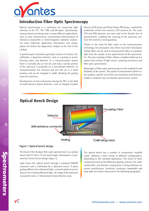
Devices (CCD) Arrays and Photo Diode (PD) Arrays, enabled the production of low cost scanners, CCD cameras etc. The same CCD and PDA detectors are now used in the Avantes line of spectrometers, enabling fast scanning of the spectrum, wit-hout the need of a moving grating.Thanks to the need for fiber optics in the communication technology, low absorption silica fibers have been developed. Similar fibers can be used as measurement fibers to transport light from the sample to the optical bench of the spectrome-ter. The easy coupling of fibers allows a modular build-up of a system that consists of light source, sampling accessories and fiber optic spectrometer.Advantages of fiber optic spectroscopy are the modularity and flexibility of the system. The speed of measurement allows in-line analysis, and the use of low-cost commonly used detectors enable a complete low cost Avantes spectrometer system.Optical spectroscopy is a technique for measuring light intensity in the UV-, VIS-, NIR- and IR-region. Spectroscopic measurements are being used in many different applications, such as color measurement, concentration determination of chemical components or electromagnetic radiation analysis. For more elaborate application information and setups, please see further the Application chapter at the end of this catalog.A spectroscopic instrument generally consists of entrance slit, collimator, a dispersive element, such as a grating or prism, focusing optics and detector. In a monochromator system there is normally also an exit slit, and only a narrow portion of the spectrum is projected on a one-element detector. In monochromators the entrance and exit slits are in a fixed position and can be changed in width. Rotating the grating scans the spectrum.Development of micro-electronics during the 90’s in the field of multi-element optical detectors, such as Charged Coupledmetrical Czerny-Turner design (figure 1).Light enters the optical bench through a standardSMA905 connector and is collimated by a spherical mirror. A plane grating diffracts the collimated light; a second spherical mirror focuses the resulting diffracted light. An image of the spectrum is projected onto a 1-dimensional linear detector array.installed configurations, depending on the intended application. The choice of these components such as the diffraction grating, entrance slit, order sorting filter, and detector coating have a strong influence on system specifications. Sensitivity, resolution, bandwidth and stray light are further discussed in the following paragraphs.Introduction Fiber Optic SpectroscopySpectrometersinfo@ • S p e c t r o m e t e r s •info@Biomedical Technology Chemistry Colorimetry Food Technology Inline Process Control Radiometry Thinfilm AnalysisHow to configure a spectrometer for your application?For optimal UV sensitivity we recommend the back-thinned UV sensitive CCD detector, as implemented in the AvaSpec-2048x14.For the different detector types the photometric sensitivity is given in table 4, the spectral sensitivity for each detector is depicted in figure 5.b. Chemometric SensitivityTo detect two absorbance values, close to each other with maximum sensitivity you need a high Signal to Noise (S/N) performance. The detector with best S/N performance is the 2048x14 pixel back-thinned CCD detector, next to the 256/1024 CMOS detector in the AvaSpec-256/1024. The S/N performance can also be enhanced by averaging over multiple spectra.4. Timing and SpeedThe data capture process is inherently fast with detector arrays and no moving parts. However there is an optimal detector for each application. For fast response applications, we recommend to use the AvaSpec- USB2 platform spectrometers. When datatransfer time is critical we recommend to select a small amount of pixels to be transferred with the UBS2 interface. Data transfer time can be enhanced by selecting the pixel range of interest to be transmitted to the PC; in general the AvaSpec-128 may be considered as the fastest spectrometer with more than 8000 scans per second.The above parameters are the most important in choosing the right spectrometer configuration, please contact our application engi-neers to optimize and fine-tune the system to your needs. On the next page you will find a quick reference table 1 for most common applications, for a more elaborate explanation and configurations, please refer to the applications section in the back of this catalog.In addition we have introduced in this catalog application icons, that will help you to find the right products and accessories for your applications.In the modular AvaSpec design a number of choices have to be made on several optical components and options, depending on the application you want to use the spectrometer for.This section should give you some guidance on how to choose the right grating, slit, detector and other options, installed in the AvaSpec.1. Wavelength RangeIn the determination for the optimal configuration of a spectrometer system the wavelength range is the first important parameter that defines the grating choice. If you are looking for a wide wavelength range, we recommend to take an A-type (300 lines/mm) or B-type (600 lines/mm) grating (see Grating selection table in the spectrometer product section). The other important component is the detector choice, Avantes offers 9 different detector types with each different sensitivity curves (see figure 5). For UV applications the new 2048x14 pixel back-thinned CCD detector, the 256/1024 pixel CMOS detectors or DUV- enhanced 2048 or 3648 pixel CCD detectors may be selected. For the NIR range 3 different InGaAs detectors are available.If you want to combine a wide range with a high resolu-tion, a multiple channel spectrometer may be the best choice.2. Optical ResolutionIf you desire a high optical resolution we recommend to pick a grating that has 1200 or more lines/mm (C,D,E or F types) in combination with a narrow slit and a detector with 2048 or 3648 pixels, for example 10 µm slit for the best resolution on the AvaSpec-2048 (see Resolution table in the spectrometer product section)3. SensitivityTalking about sensitivity, it is very important to distinguish between photometric sensitivity (How much light do I need for a detectable signal?) and chemometric sensitivity (What absorbance difference level can still be detected?) a. Photometric SensitivityIn order to achieve the most sensitive spectrometer in for example Fluorescence or Raman applications we recommend the 2048 pixel CCD detector, as in the AvaSpec-2048. Further we recommend the use of a DCL-UV/VIS detector collection lens, a relatively wide slit (100µm or wider) or no slit and an A type grating. For an A-type grating (300 lines/mm) the light dispersion is minimal, so it has the highest sensitivity of the grating types. Optionally the Thermo-electric cooling of the CCD detector (see product section AvaSpec-2048-TEC, page 30) may be chosen to minimize noise and increase dynamicrange at long integration times (60 seconds).Table 1 Quick reference guide for spectrometer configurationApplication AvaSpec- Grating WL range (nm) Coating SlitFWHM DCL OSF OSCtype Resolution (nm)Biomedical 2048 NB 500-1000 - 50 1.2 - 475 -Chemometry 1024 UA 200-1100 - 50 2.0 - - OSC-UA 128 VA 360-780 - 100 6.4 X/- - -Color 256 VA 360-780 - 50 3.2 - - -2048 BB 360-780 - 200 4.1 X/- - -Fluorescence 2048 VA 350-1100 - 200 8.0 X - OSC Fruit-sugar 128 IA 800-1100 - 50 5.4 X 600 -Gemology 2048 VA 350-1100 - 25 1.4 X - OSC High 2048 VD 600-700 - 10 0.07 - 550 -resolution 3648 VD 600-700 - 10 0.05 - 550 -High UV- 2048x14UC200-450-2002.0---Sensitivity Irradiance 2048 UA 200-1100 DUV 50 2.8 X/- - OSC-UA Laserdiode 2048 NC 700-800 - 10 0.1 - 600 -LED 2048 VA 350-1100 - 25 1.4 X/- - OSC LIBS 2048FT UE 200-300 DUV 10 0.09 - - - 2048USB2 UE 200-300 DUV 10 0.09 - - -Raman 2048TEC NC 780-930 - 25 0.2 X 600 -Thin Films 2048 UA 200-1100 DUV - 4.1 X - OSC-UA UV/VIS/NIR 2048 UA 200-1100 DUV 25 1.4 X/- - OSC-UA 2048x14UA200-1100 - 25 1.4 - - OSC-UA NIR NIR256-1.7 NIRA 900-1750 - 50 5.0 - 1000 - NIR256-2.2 NIRZ 1200-2200 - 50 10.0 - 1000 -NIR256-2.5 NIRY1000-2500-5015.0-1000-info@ • Spectrometers9S p e c t r o m e t e r s • info@For each spectrometer type, a grating selection table is shown in the Spectrometer Platforms section. Table 2 illustrates how to read the grating selection table. The spectral range to select in Table 2 depends on the starting wavelength of the grating Please select Spectral range band-width from the useable Wavelength range, for example: grating UE (200-315nm)*the spectral range depends on the starting wavelength of the grating; the higher the wave-length, the smaller the range.For example grating UE (510-580 nm)The order code is defined by 2 letters: the first is the Blaze (U= 250/300nm or UV for holo-graphic, B=400nm, V=500nm or VIS for holo-graphic, N=750nm, I=1000nm) and the second the nr of lines/mm (Z=150, A=300, B=600, C=1200, D=1800, E=2400, F=3600 lines/mm)Spectrometersinfo@ •Figure 2 Grating Efficiency Curves 300 Lines/mm Gratings600 Lines/mm Gratings1200 Lines/mm Gratings 1800 Lines/mm Gratings2400 Lines/mm Gratings3600 Lines/mm GratingsSpectrometers •info@Figure 3 Grating Dispersion Curves300 Lines/mm Gratings600 Lines/mm Gratings1200 Lines/mm Gratings1800 Lines/mm Gratings2400 Lines/mm Gratings3600 Lines/mm Gratingsinfo@ •SpectrometersThe optical resolution is defined as the minimum difference in wavelength that can be separated by the spectrometer. For separation of two spectral lines it is necessary to image them at least 2 array-pixels apart. Because the grating determines how far different wavelengths are separated (dispersed) at the detector array, it is an important variable for the resolution.The other important parameter is the width of the light beam entering the spectrometer. This is basically the instal-led fixed entrance slit in the spectrometer, or the fiber core diameter when no slit is installed.The slits can be installed with following dimensions: 10, 25 or 50 x 1000 µm high or 100, 200 or 500 µm x 2000 µm high. Its image on the detector array for a given wavelength will cover a number of pixels. For two spectral lines to be separated, it is now necessary that they be dispersed over at least this image size plus one pixel. When large core fibers are used the resoluti-on can be improved by a slit of smaller size than the fiber core. This effectively reduces the width of the entering light beam. The influence of the chosen grating and the effective width of the light beam (fiber core or entrance slit) are shown in the tables at the product information. In Table 3 the typical reso-lution can be found for the AvaSpec-2048. Please note that for the higher lines/mm gratings the pixel dispersion varies along the wavelength range and gets better towards the lon-ger wavelengths (see also Figure 3). The best resolution can always be found for the longest wavelengths. The resolution in this table is defined as F(ull) W(idth) H(alf) M(aximum), which is defined as the width in nm of the peak at 50% of the maximum intensity (see Figure 4).Graphs with information about the pixel dispersion can be found in the gratings section as well, so you can optimally determine the right grating and resolution for your specific application.In combination with a DCL-detector collection lens or thick fibers the actual FWHM value can be 10-20% higher than the value in the table. For best resolution small fibers and no DCLFigure 4 Full Width Half MaximumHow to select optimal Optical Resolution?Slit size (µm)Grating (lines/mm) 10 25 50 100 200 500 300 0.8 1.4 2.4 4.3 8.0 20.0600 0.4 0.7 1.2 2.1 4.1 10.01200 0.1-0.2* 0.2-0.3* 0.4-0.6* 0.7-1.0* 1.4-2.0* 3.3-4.8*1800 0.07-0.12* 0.12-0.21* 0.2-0.36* 0.4-0.7* 0.7-1.4* 1.7-3.3*2400 0.05-0.09* 0.08-0.15* 0.14-0.25* 0.3-0.5* 0.5-0.9* 1.2-2.2*36000.04-0.06*0.07-0.10*0.11-0.16*0.2-0.3*0.4-0.6*0.9-1.4**depends on the starting wavelength of the grating; the higher the wavelength, the bigger the dispersion and the better the resolutionTable 3 Resolution (FWHM in nm) for the AvaSpec-2048Installed Slit in SMA AdapterS p e c t r o m e t e r s •info@The AvaSpec spectrometers can be equipped with several types of detector arrays. Presently we offer silicon-based CCD, back-thinned CCD, CMOS and Photo Diode Arrays for the 200-1100 nm range. A complete overview is given in the next sec-tion “Sensitivity” in table 4. For the NIR range (1000-2500nm) InGaAs arrays are implemented.CCD Detectors (AvaSpec-2048/3648)The Charged Coupled Device (CCD) detector stores the charge, dissipated as photons strike the photoactive surface. At the end of a controlled time-interval (integration time), the remaining charge is transferred to a buffer and then this signal is being transferred to the AD converter. CCD detectors are naturally integrating and therefore have an enormous dynamic range, only limited by the dark (thermal) current and the speed of the AD converter. The 3648 pixel CCD has an integrated electronic shutter function, so an integration time of 10µsec can be achieved.+ Advantages for the CCD detector are many pixels (2048 or 3648), high sensitivity and high speed.- Main disadvantage is the lower S/N ratio.UV enhancementFor applications below 350 nm with the AvaSpec-2048/3648 a special DUV-detector coating is required. The uncoated CCD-response below 350 nm is very poor; the DUV lumo-gen coating enhances the detector response in the region 150-350nm. The DUV coating has a very fast decay time, typ. in ns range and is therefore useful for fast trigger LIBS applications.Back-thinned CCD Detectors (AvaSpec-2048x14)For applications requiring high quantum efficiency in the UV (200-350nm) and NIR (900-1160nm) range, combined with good S/N and a wide dynamic range, the new back-thinned CCD detector may be the right choice. The detector is an area detector of 2048x14 pixels, for which the vertical 14 pixels are binned (electronically added together) to have more sensiti-vity and a better S/N performance. + A dvantage of the back-thinned CCD detector is the good UV and NIR sensitivity, combined with good S/N and dynamic range- Disadvantage is the relative high costPhoto Diode Arrays (AvaSpec-128)A silicon photodiode array consists of a linear array of mul-tiple photo diode elements, for the AvaSpec-128 this is 128 pixels. Each pixel consists of a P/N junction with a positively doped P region and a negatively doped N region. When light enters the photodiode, electrons will become excited and output an electrical signal. Most photodiode arrays have anDetector Arraysintegrated signal processing circuit with readout/integration amplifier on the same chip.+ Advantages for the Photodiode detector are high NIR sensitivity and high speed.- Disadvantages are limited amount of pixels and no UV response.CMOS linear image sensors (AvaSpec-256/1024)These so called CMOS linear image sensors have a lower charge to voltage conversion efficiency than CCD array sensors and are therefore less light sensitive, but have a much better signal to noise ratio.The CMOS detectors have a higher conversion gain than NMOS detectors and also have a clamp circuit added to the internal readout circuit to suppress noise to a low level.+ Advantages for the CMOS detectors are good S/N ratio and good UV sensitivity.- Disadvantages are the low readout speed, low sensitivity, and relative high cost (1024 pixels).InGaAs linear image sensors (AvaSpec-NIR256)The InGaAs linear image sensors deliver high sensitivity in the NIR wavelength range. The detector consists of a charge ampli-fier array with CMOS transistors, a shift register and timing generator. 3 versions of detectors are available:• 256 pixel non-cooled InGaAs detector for the 900-1750nm useable range • 256 pixel 2-stage cooled Extended InGaAs detector for the 1000-2200nm range • 256 pixel 2-stage cooled Extended InGaAs detector for the1000-2500nm rangeDifferent Detector ArraysSensitivityThe sensitivity of a detector pixel at a certain wavelength is defined as the detector electrical output per unit of radia-tion energy (photons) incident to that pixel. With a given A/D converter this can be expressed as the number of counts per mJ of incident radiation.The relation between light energy entering the optical bench and the amount hitting a single detector pixel depends on the optical bench configuration. The efficiency curve of the grating used, the size of the input fiber or slit, the mirror performance and the use of a Detector Collection Lens are the main parameters. With a given set-up it is possible to do measurements over about 6-7 decades of irradiance levels. Some standard detector specifications can be found in Table 4 detector specifications. Optionally a cylindrical Detector Collection Lens (DCL) can be mounted directly on the detec-tor array. The quartz lens (DCL-UV for AvaSpec-2048/3648) will increase the system sensitivity by a factor of 3-5, depen-ding on the fiber diameter used.In Table 4 the overall sensitivity is given for the detector types currently used in the UV/VIS AvaSpec spectrometers as output in counts per ms integration time for a 16-bit AD converter. To compare the different detector arrays we have assumed an optical bench with 600 lines/mm grating and no DCL. The entrance of the bench is an 8 µm core diameter fiber, con-nected to a standard AvaLight-HAL halogen light source. This is equivalent to ca. 1 µWatt light energy input.In table 5 the specification is given for the NIR spectrometers, in figure 5 and figure 6 the spectral response curve for the dif-ferent detector types are depicted.info@ •SpectrometersTable 4 Detector specifications (based on a 16-bit AD converter)Detector TAOS 128 HAM256 HAM1024 SONY2048 TOSHIBA3648 HAM2048x14Type Photo diode array CMOS linear array CMOS linear array CCD linear array CCD linear array Back-thinnedCCD Array # Pixels, pitch 128, 63.5 µm 256, 25 µm 1024, 25 µm 2048, 14 µm 3648, 8 µm 2048x14, 14 µmpixel width x 55.5 x 63.5 25 x 500 25 x 500 14 x 56 8 x 200 14x14 (totalheight (µm)height 196 µm)pixel well depth 250,000 4,000,000 4,000,000 40,000 120,000 250,000(electrons)Sensitivity 100 22 22 240 160 200V/lx.sSensitivity 100 440 440 40 60 50Photons/count@600nmSensitivity 4000 120 120 20,000 14,000 16,000(AvaLight-HAL, (AvaSpec-128) (AvaSpec-256) (AvaSpec-1024) (AvaSpec-2048) (AvaSpec-3648) (Avaspec 2048x14)8 µm fiber)in counts/µW perms integration timePeak wavelength 750 nm 500 nm 500 nm 500 nm 550 nm 650 nmSignal/Noise 500:1 2000 :1 2000 :1 200 :1 350 :1 500:1Dark noise 60 28 60 35 35 50(counts RMS)Dynamic Range 1000 2500 2500 2000 2000 1300PRNU**± 4% ± 3% ±3% ± 5% ± 5% ± 3%Wavelength range 360-1100 200-1000 200-1000 200*-1100 200*-1100 200-1160(nm)Frequency 2 MHz 500 kHz 500 kHz 2 MHz 1 MHz 1.5 MHz* DUV coated** Photo Response Non-Uniformity = max difference between output of pixels when uniformly illuminated, divided by average signalS p e c t r o m e t e r s • info@Figure 5 Detector Spectral sensitivity curves Table 5 NIR Detector SpecificationsDetectorNIR256-1.7 NIR256-2.2NIR256-2.5TypeLinear InGaAs array Linear InGaAs array Linear InGaAs arraywith 2 stage TE cooling with 2 stage TE cooling # Pixels, pitch 256, 50 µm 256, 50 µm 256, 50 µm pixel width x 50 x 50050 x 500 50 x 500height (µm)Pixel well depth 16,000,000 1,500,000 1,500,000(electrons)Sensitivity 350250200(AvaLight-HAL, 8 µm fiber)in counts/µW per ms integration timePeak wavelength 1550 nm 2000 nm 2300 nmSignal/Noise 4000:1 1200 :1 1200 :1Dark noise 12 40 40 (counts RMS)Dynamic Range 5000 1600 1600PRNU** ± 5% ± 5% ± 5%Defective pixels 012 12(max)Wavelength range 900-1750 1000-2200 1000-2500 (nm)Frequency500 kHz500 kHz500 kHz** Photo Response Non-Uniformity = max difference between output of pixels when uniformly illuminated, divided by average signalFigure 6 NIR Detector Sensitivity CurvesSpectrometers Stray light is radiation of the wrong wavelength that activatesa signal at a detector element. Sources of stray light can be:• Ambient light• Scattering light from imperfect optical components orreflections of non-optical components• Order overlapEncasing the spectrometer in a light tight housing eliminatesambient stray light.When working at the detection limit of the spectrometersystem, the stray light level from the optical bench, gratingand focusing mirrors will determine the ultimate limit ofdetection. Most gratings used are holographic gratings,known for their low level of stray light. Stray light measure-ments are being carried out with a laser light, shining into theoptical bench and measuring light intensity at pixels far awayfrom the laser projected beam. Other methods use a halogenlight source and long pass- or band pass filters.Typical stray light performance is <0.05 % at 600 nm; <0.10% at 435 nm; <0.10 % at 250 nm.Second order effects, which can play an important role forgratings with low groove frequency and therefore a widewavelength range, are usually caused by the grating 2ndorder diffracted beam. The effects of these higher orders canoften be ignored, but sometimes need to be taken care of.The strategy is to limit the light to the region of the spectra,where order overlap is not possible. Second order effectscan be filtered out, using a permanently installed long-passoptical filter in the SMA entrance connector or an order sor-ting coating on a window in front of the detector. The ordersorting coatings on the window typically have one long passfilter (590nm) or 2 long pass filters (350 nm and 590 nm),depending on the type and range of the selected grating.In Table 6 a wide range of optical filters for installation in theoptical bench can be found. The use of following long-passfilters is recommended: OSF-475 for grating NB and NC, OSF-515/550 for grating NB and OSF-600 for grating IB.In addition to the order sorting coatings we implement partialDUV coatings on Sony 2048 and Toshiba 3648 detectors toavoid second order effects from UV response and to enhancesensitivity and decrease noise in the Visible range.This partial DUV coating is done automatically for the follo-wing grating types:• UA for 200-1100 nm, DUV400, only first 400 pixelscoated• UB for 200-700 nm, DUV800, only first 800 pixelscoatedStray Light and Second Order EffectsTable 6 Filters installed in the AvaSpec spectrometer seriesOSF-385Permanently installed 1 mm order sorting filter @ 371 nmOSF-475 Permanently installed 1 mm order sorting filter @ 466 nmOSF-515 Permanently installed 1 mm order sorting filter @ 506 nmOSF-550 Permanently installed 1 mm order sorting filter @ 541 nmOSF-600 Permanently installed 1 mm order sorting filter @ 591 nmOSC Order sorting coating with 590nm long pass filter for VA, BB (>350 nm) and VB gratingsin AvaSpec-1024/2048/3648/2048x14OSC-UA Order sorting coating with 350 and 590nm longpass filter for UA gratingsin AvaSpec-1024/2048/3648/2048x14OSC-UB Order sorting coating with 350 and 590nm longpass filter for UB or BB (<350 nm) gratingsin AvaSpec-1024/2048/3648/2048x14Order Sorting Window in holderinfo@ • Product name Electronics Optical bench Detector Housing AvaSpec-128 AS-161 with USB AvaBench-45, allgratings 360-1100 nm TAOS 128AvaSpec-128-USB2 AS-5216 with USB2AvaSpec-256 AS-161 with USB AvaBench-45, allgratings 200-1100 nm HAM 256AvaSpec-256-USB2 AS-5216 with USB2AvaSpec-1024 AS-161 with USB AvaBench-75, allgratings 200-1100 nm HAM 1024AvaSpec-1024-USB2 AS-5216 with USB2AvaSpec-2048 AS-161 with USB AvaBench-75, allgratings 200-1100 nm Sony 2048AvaSpec-2048-USB2 AS-5216 with USB2AvaSpec-3648-USB2 AS-5216 with USB2 AvaBench-75, Toshiba 3648all gratings 200-1100 nmAvaSpec-2048x14-USB2 AS-5216 with USB2 AvaBench-75, HAM 2048x14all gratings 200-1160 nmAvaSpec-NIR256-1.7 AS-5216 with USB2 AvaBench-50, HAM NIR256-1.7grating 900-1750 nmAvaSpec-NIR256-2.2 AS-5216 with USB2 AvaBench-50, HAM NIR256-2.2grating 1000-2200 nmAvaSpec-NIR256-2.5 AS-5216 with USB2 AvaBench-50, HAM NIR256-2.5grating 1000-2500 nmAvaSpec-xxx-2 AS-161 with USB, 2 channels AvaBench-45/75, all TAOS 128xxx = 102/256/1024/ gratings 200-1100 nm HAM 256/10242048 or Sony 2048AvaSpec Multichannel AS-161 with USB1 or AvaBench-45/75, All detectorsas Desktop AS-5216 with USB2 all gratings 200-1100 nmor Rackmount17S p e c t r o m e t e r s • info@。
Quant-iT
Quant-iT ™ 1X dsDNA HS Assay KitCatalog No. Q33232Product informationThe Quant-iT ™ 1X dsDNA HS (High Sensitivity) Assay Kit makes DNA quantitation easy and accurate. The kit includes a ready-to-use assay buffer and DNA standards. To perform the assay, dilute your sample (any volume from 1–20 μL is acceptable) into the 1X working solution provided, then read the concentration using a fluorescence plate reader. The assay is highly selective for double-stranded DNA (dsDNA) over RNA (Figure 4, page 6) and is accurate for initial sampleconcentrations from 10 pg/μL to 100 ng/μL, providing a core detection range of 0.2 ng to 100 ng of DNA in the assay tube. The assay is performed at room temperature, and the signal is stable for 3 hours when the samples are protected from light. Common contaminants such as salts, free nucleotides, solvents, detergents, or protein are well tolerated in the assay (Table 2, page 7).In addition to the Quant-iT ™ 1X dsDNA HS Assay Kit described here, we also offer the Quant-iT ™ 1X dsDNA BR (Broad Range) Assay Kit (Cat. No. Q33267). The Quant-iT ™ 1X dsDNA BR Assay Kit is designed for assaying samples containing 4–2000 ng of DNA. The Qubit ™ dsDNA HS Assay – Lambda standard (Cat. No. Q33233) can be used to create the standard dilution series for the Quant-iT ™ dsDNA HS assay.If you would like to use this kit with the Qubit ™ Fluorometer, we have included instructions under "Perform the Quant-iT ™ 1X dsDNA HS Assay on a Qubit ™ Fluorometer" (page 4).Table 1.Contents and storagePub. No. MAN0017526Rev. C.0Critical assay parametersAssay temperatureThe Quant-iT ™ 1X dsDNA HS Assay delivers optimal performance when all solutions are at room temperature (18–28˚C). Temperature fluctuations can influence the accuracy of the assay (Figure 5, page 6).To minimize temperature fluctuations, insert all assay tubes into the fluorescence microplate reader only for as much time as it takes for the instrument to measure the fluorescence. Do not hold the assay tubes in your hand before reading because this warms the solution and results in a different reading.Incubation timeTo allow the Quant-iT ™ 1X dsDNA HS Assay to reach optimal fluorescence, incubate the tubes for 2 minutes after mixing the sample or the standard with the working solution. After this incubation period, the fluorescence signal is stable for 3 hours at room temperature when samples are protected from light.Photostability of Quant-iT ™reagentsThe Quant-iT ™ reagents exhibit high photostability, showing <0.3% drop in fluorescence after 9 readings and <2.5% drop in fluorescence after 40 readings.Handling and disposalNo data are currently available that address the mutagenicity or toxicity of theQuant-iT ™ 1X dsDNA HS Reagent (the dye in Component A). This reagent is known to bind nucleic acids. Treat the Quant-iT ™ 1X dsDNA HS working solution with the same safety precautions as all other potential mutagens and dispose of the dye in accordance with local regulations.Figure 1. Excitation and emission maxima for the Quant-iT ™1X dsDNA HS reagent when bound to dsDNA.Perform the Quant-iT™ dsDNA HS Assay on a fluorescence microplate readerThis protocol describes the use of the Quant-iT™ 1X dsDNA HS Assay Kit with afluorescence microplate reader that is equipped with either a monochrometer orexcitation and emission filters appropriate for fluorescein or Alexa Fluor™ 488 dye(Figure 1, page 2). Some contaminating substances may interfere with the assay; formore information, see "Contaminants tolerated by the Quant-iT™ 1X dsDNA HS Assay"(page 7). For an overview of this procedure, see Figure 2.Figure 2. The Quant-iT™ dsDNA High-Sensitivity assay.Assay procedure IMPORTANT! For best results, ensure that all materials and reagents are at roomtemperature.1.1 Add 10 μL of each Quant-iT™ 1X dsDNA HS Standard to separate wells. Duplicates ortriplicates of the standards are recommended.1.2 Add 1–20 µL of each unknown DNA sample to separate wells. Duplicates or triplicatesof the unknown samples are recommended.1.3 Load 200 μL of the Quant-iT™ 1X dsDNA working solution into each microplate well.This can be done readily using a multichannel pipettor.If possible, mix your 96-well plate using a plate mixer or using the plate reader for1.4about 3–10 seconds. Following mixing, allow the plate to incubate at room temperaturefor 2 minutes..Measure the fluorescence using a microplate reader (excitation/emission maxima are1.5502/523 nm; see Figure 1, page 2). Standard fluorescein wavelengths (excitation/emission at ~480/530 nm) are appropriate for this dye. The fluorescence signal is stablefor 3 hours at room temperature when protected from light.Use a standard curve to determine the DNA amounts. For the dsDNA standards, plot1.6amount vs. fluorescence, and fit a straight line to the data points.Note: Many curve fitting programs will calculate the y-intercept. However, for bestresults, manually set the y-intercept as the RFU value obtained from the 0 ng/μLdsDNA standard.Data analysis considerations –standard curves and extendedranges The fluorescence of the Quant-iT™ 1X dsDNA HS reagent bound to dsDNA is extremelylinear from 0–100 ng. For best results at the low end of the standard curve, the lineshould be forced through the background point (or through zero, if backgroundhas been subtracted). When 10 μL volumes of the standards are used, the lowestDNA-containing standard represents 5 ng of DNA; nevertheless, highly accuratedeterminations of DNA down to 0.2 ng are attained using the standard curve asdescribed above.To assess the reliability of the assay in the low range, use smaller volumes of thestandards; for example, 2 μL volumes for a standard curve ranging from 0–20 ng.Alternatively, dilute the standards in buffer for an even tighter range. Duringdevelopment of the Quant-iT™ 1X dsDNA HS assay, we were able to detect 0.05 ng ofλ DNA under ideal experimental circumstances (using calibrated pipettors, octuplicatedeterminations, the best microplate readers, and Z-factor1 analysis). Your results mayvary.If desired, the utility of the Quant-iT™ 1X dsDNA HS assay can be extended beyond100 ng, up to 200 ng. For standards in this range, use 20 μL volumes of the providedstandards. Note that the standard curve may not be linear in the range 160–200 ng, andhigh levels of RNA may now interfere slightly with the results.Perform the Quant-iT™ dsDNA HS Assay on a Qubit™ FluorometerThe Quant-iT™ 1X dsDNA Assay Kit can be adapted for use with the Qubit™Fluorometer. The protocol below is abbreviated from the Qubit™ Fluorometer userguide, which is available at /qubit. Although a step-by-step protocoland critical assay parameters are given here, more detail is available in the Qubit™Fluorometer user guide and you are encouraged to familiarize yourself with thismanual before you begin your assay. See Figure 3 for an overview of the procedure.Figure 3. Overview for using the Quant-iT™ 1X dsDNA HS assay in the Qubit™ fluorometer.Assay procedure IMPORTANT! For best results, ensure that all materials and reagents are at roomtemperature.2.1 Set up the required number of 0.5-mL tubes for standards and samples. The Quant-iT™1X dsDNA HS Assay requires 2 standards.Note: Use only thin-wall, clear, 0.5-mL PCR tubes. Acceptable tubes include Qubit™assay tubes (Cat. No. Q32856).2.2 Label the tube lids.Note: Do not label the side of the tube as this could interfere with the sample read. Labelthe lid of each standard tube correctly. Calibration of the Qubit™ Fluorometer requiresthe standards to be inserted into the instrument in the right order.2.3 Add 10 µL of the 0 ng/μL and the 10 ng/μL Quant-iT™ 1X dsDNA HS Standard to theappropriate tube2.4 Add 1–20 µL of each user sample to the appropriate tube.2.5 Add the Quant-iT™ 1X dsDNA HS Working Solution to each tube such that the finalvolume is 200 µL.Note: The final volume in each tube must be 200 µL. Each standard tube requires 190 µLof Quant-iT™ working solution, and each sample tube requires anywhere from180–199 µL.2.6 Mix each sample vigorously by vortexing for 3–5 seconds.2.7 Allow all tubes to incubate at room temperature for 2 minutes, then proceed to read thestandards and samples. Follow the procedure appropriate for your instrument:• Qubit™ Flex Fluorometer• Qubit™ 4 Fluorometer• Qubit™ 3 FluorometerNote: If you are using the Qubit™ 3 Fluorometer, download the 1X dsDNA algorithmand assay button from /qubit, then install it onto your Qubit™Fluorometer.AppendixSelectivity of the Quant-iT™ 1XdsDNA HS AssayFigure 4. DNA selectivity and sensitivity of the Quant-iT™ 1X dsDNA HS Assay (Cat. No. Q33232). Triplicate10-μL samples of λ DNA, E. coli rRNA, or a 1:1 mixture of DNA and RNA were assayed with the Quant-iT™1X dsDNA HS Assay. Fluorescence was measured at 502/532 nm and plotted versus the concentration ofthe RNA or DNA sample alone, or versus the mass of the DNA component in the 1:1 mixture. The variation(CV) of replicate DNA determinations was ≤2%. The inset is an expanded view of the low range of the assayshowing the extreme sensitivity of the assay for DNA. Background fluorescence has not been subtracted.Effect of temperature on theQuant-iT™ 1X dsDNA HSAssayFigure 5. Plot of fluorescence vs. temperature for the Quant-iT™ 1X dsDNA HS Assay. The Quant-iT™assays are designed to be performed at room temperature, as temperature fluctuations can influence theaccuracy of the assay.Contaminants tolerated by the Quant-iT ™ 1X dsDNA HSAssayNote: While the contaminant tolerances of the Quant-iT ™ 1X dsDNA HS assay and theQuant-iT ™ dsDNA HS assay are largely similar, they are not identical.Reference1. J Biomol Screen 4, 67–73 (1999).Table 2. Effect of contaminants in the Quant-iT ™1X dsDNA HS Assay*/support | /askaquestion Limited Product WarrantyLife Technologies Corporation and/or its affiliate(s) warrant their products as set forth in the Life Technologies’ General Terms and Conditions of Sale found on Life Technologies’ website at /us/en/home/global/terms-and-conditions.html . If you have any questions, please contact Life Technologies at /support .Life Technologies Corporation | 29851 Willow Creek Road | Eugene, OR 97402 USAFor descriptions of symbols on product labels or prodoct documents, go to /symbols-definition .The information in this guide is subject to change without notice.DISCLAIMER: TO THE EXTENT ALLOWED BY LAW, LIFE TECHNOLOGIES AND/OR ITS AFFILIATE(S) WILL NOT BE LIABLE FOR SPECIAL, INCIDENTAL,INDIRECT, PUNITIVE, MULTIPLE OR CONSEQUENTIAL DAMAGES IN CONNECTION WITH OR ARISING FROM THIS DOCUMENT, INCLUDING YOUR USE OF IT.Important Licensing Information: These products may be covered by one or more Limited Use Label Licenses. By use of these products, you accept the terms and conditions of all applicable Limited Use Label Licenses.Revision history:Pub. No. MAN0017526©2021 Thermo Fisher Scientific Inc. All rights reserved. All trademarks are the property of Thermo Fisher Scientific and its subsidiaries unless otherwise specified .Ordering informationCat. No. Product name Unit size Q33232Quant-iT™ 1X dsDNA HS Assay Kit.................................................................... 1 kitRelated products Q33267 Quant-iT™ 1X dsDNA BR Assay Kit.................................................................... 1 kit Q33120 Quant-iT™ dsDNA Assay Kit, High Sensitivity............................................................ 1 kit Q33130 Quant-iT™ dsDNA Assay Kit, Broad Range.............................................................. 1 kit Q10213 Quant-iT™ RNA Assay Kit, Broad Range................................................................ 1 kit Q33140 Quant-iT™ RNA Assay Kit, 1000 assays ................................................................ 1 kit Q32882 Quant-iT™ microRNA Assay Kit, 1000 assays............................................................ 1 kit Q33210 Quant-iT™ Protein Assay Kit, 1000 assays .............................................................. 1 kit O11492 Quant-iT™ OliGreen™ ssDNA Assay Kit ................................................................ 1 kit Q33233 Qubit™ 1X dsDNA Assay- Lambda Standard ............................................................ 1 kit Q33238 Qubit™ 4 Fluorometer with WiFi....................................................................... 1 each Q33327 Qubit™ Flex Fluorometer ............................................................................ 1 each Q33252 Qubit™ Flex Assay Tube Strips .................................................................. 125 tube strips M33089 Microplates for fluorescence-based assays, 96-well (black-walled, clear bottom) ................................ 10 plates。
Handbook_of_X-Ray_Spectrometry_CH01

1X-ray PhysicsAndrzej A.MarkowiczVienna,AustriaI.INTRODUCTIONIn this introductory chapter,the basic concepts and processes of x-ray physics that relate to x-ray spectrometry are presented.Special emphasis is on the emission of the continuum and characteristic x-rays as well as on the interactions of photons with matter.In the latter,only major processes of the interactions are covered in detail,and the cross sections for different types of interactions and the fundamental parameters for other processes involved in the emission of the characteristic x-rays are given by the analytical expressions and=or in a tabulated form.Basic equations for the intensity of the characteristic x-rays for the different modes of x-ray spectrometry are also presented(without derivation). Detailed expressions relating the emitted intensity of the characteristic x-rays to the concentration of the element in the specimen are discussed in the subsequent chapters of this handbook dedicated to specific modes of x-ray spectrometry.II.HISTORYX-rays were discovered in1895by Wilhelm Conrad Ro ntgen at the University of Wu rzburg,Bavaria.He noticed that some crystals of barium platinocyanide,near a dis-charge tube completely enclosed in black paper,became luminescent when the discharge occurred.By examining the shadows cast by the rays.Ro ntgen traced the origin of the rays to the walls of the discharge tube.In1896,Campbell-Swinton introduced a definite target (platinum)for the cathode rays to hit;this target was called the anticathode.For his work x-rays,Ro ntgen received thefirst Nobel Prize in physics,in1901.It was thefirst of six to be awarded in thefield of x-rays by1927.The obvious similarities with light led to the crucial tests of established wave optics: polarization,diffraction,reflection,and refraction.With limited experimental facilities, Ro ntgen and his contemporaries couldfind no evidence of any of these;hence,the des-ignation‘‘x’’(unknown)of the rays,generated by the stoppage at anode targets of the cathode rays,identified by Thomson in1897as electrons.The nature of x-rays was the subject of much controversy.In1906,Barkla found evidence in scattering experiments that x-rays could be polarized and must therefore by waves,but W.H.Bragg’s studies of the produced ionization indicated that they werecorpuscular.The essential wave nature of x-rays was established in1912by Laue, Friedrich,and Knipping,who showed that x-rays could be diffracted by a crystal(copper sulfate pentahydrate)that acted as a three-dimensional diffraction grating.W.H.Bragg and W.L.Bragg(father and son)found the law for the selective reflection of x-rays.In 1908,Barkla and Sadler deduced,by scattering experiments,that x-rays contained com-ponents characteristic of the material of the target;they called these components K and L radiations.That these radiations had sharply defined wavelengths was shown by the diffraction experiments of W.H.Bragg in1913.These experiments demonstrated clearly the existence of a line spectrum superimposed upon a continuous(‘‘White’’)spectrum.In 1913,Moseley showed that the wavelengths of the lines were characteristic of the element of the which the target was made and,further,showed that they had the same sequence as the atomic numbers,thus enabling atomic numbers to be determined unambiguously for thefirst time.The characteristic K absorption wasfirst observed by de Broglie and in-terpreted by W.L.Bragg and Siegbahn.The effect on x-ray absorption spectra of the chemical state of the absorber was observed by Bergengren in1920.The influence of the chemical state of the emitter on x-ray emission spectra was observed by Lindh and Lundquist in1924.The theory of x-ray spectra was worked out by Sommerfeld and others.In1919,Stenstro m found the deviations from Bragg’s law and interpreted them as the effect of refraction.The anomalous dispersion of x-ray was discovered by Larsson in 1929,and the extendedfine structure of x-ray absorption spectra was qualitatively in-terpreted by Kronig in1932.Soon after thefirst primary spectra excited by electron beams in an x-ray tube were observed,it was found that secondaryfluorescent x-rays were excited in any material ir-radiated with beams of primary x-rays and that the spectra of thesefluorescent x-rays were identical in wavelengths and relative intensities with those excited when the specimen was bombarded with electrons.Beginning in1932,Hevesy,Coster,and others investigated in detail the possibilities offluorescent x-ray spectroscopy as a means of qualitative and quantitative elemental analysis.III.GENERAL FEATURESX-rays,or Ro ntgen rays,are electromagnetic radiations having wavelengths roughly within the range from0.005to10nm.At the short-wavelength end,they overlap with g-rays,and at the long-wavelength end,they approach ultraviolet radiation.The properties of x-rays,some of which are discussed in detail in this chapter,are summarized as follows:InvisiblePropagated in straight lines with a velocity of36108m=s,as is lightUnaffected by electrical and magneticfieldsDifferentially absorbed while passing through matter of varying composition, density,or thicknessReflected,diffracted,refracted,and polarizedCapable of ionizing gasesCapable of affecting electrical properties of liquids and solidsCapable of blackening a photographic plateAble to liberate photoelectrons and recoil electronsCapable of producing biological reactions(e.g.,to damage or kill living cells and to produce genetic mutations)Emitted in a continuous spectrum whose short-wavelength limit is determined onlyby the voltage on the tubeEmitted also with a line spectrum characteristic of the chemical elementsFound to have absorption spectra characteristic of the chemical elementsIV.EMISSION OF CONTINUOUS RADIA TIONContinuous x-rays are produced when electrons,or other high-energy charged particles,such as protons or a -particles,lose energy in passing through the Coulomb field of a nucleus.In this interaction,the radiant energy (photons)lost by the electron is called bremsstrahlung (from the German bremsen ,to brake,and Strahlung ,radiation;this term sometimes designates the interaction itself).The emission of continuous x-rays finds a simple explanation in terms of classic electromagnetic theory,because,according to this theory,the acceleration of charged particles should be accompanied by the emission of radiation.In the case of high-energy electrons striking a target,they must be rapidly decelerated as they penetrate the material of the target,and such a high negative accel-eration should produce a pulse of radiation.The continuous x-ray spectrum generated by electrons in an x-ray tube is char-acterized by a short-wavelength limit l min ,corresponding to the maximum energy of the exciting electrons:l min ¼hceV 0ð1Þwhere h is Planck’s constant,c is the velocity of light,e is the electron charge,and V 0is the potential difference applied to the tube.This relation of the short-wavelength limit to the applied potential is called the Duane–Hunt law.The probability of radiative energy loss (bremsstrahlung)is roughly proportional to q 2Z 2T =M 20,where q is the particle charge in units of the electron charge e ,Z is the atomic number of the target material,T is the particle kinetic energy,and M 0is the rest mass of the particle.Because protons and heavier particles have large masses compared to the electron mass,they radiate relatively little;for example,the intensity of continuous x-rays generated by protons is about four orders of magnitude lower than that generated by electrons.The ratio of energy lost by bremsstrahlung to that lost by ionization can be approximated bym 0M 0 2ZT 1600m 0c ð2Þwhere m 0the rest mass of the electron.A.Spectral DistributionThe continuous x-ray spectrum generated by electrons in an x-ray tube (thick target)is characterized by the following features:1.Short-wavelength limit,l min [Eq.(1)];below this wavelength,no radiation isobserved.2.Wavelength of maximum intensity l max ,approximately 1.5times l min ;however,the relationship between l max and l min depends to some extent on voltage,voltage waveform,and atomic number.3.Total intensity nearly proportional to the square of the voltage and the firstpower of the atomic number of the target material.The most complete empirical work on the overall shape of the energy distribution curve for a thick target has been of Kulenkampff(1922,1933),who found the following formula for the energy distribution;I ðv Þdv ¼i aZ v 0Àv ðÞþbZ 2ÂÃdvð3Þwhere I ðn Þd n is the intensity of the continuous x-rays within a frequency range ðn ;n þdv Þ;i is the electron current striking the target,Z is the atomic number of the target material,n 0is the cutofffrequency ð¼c =l min Þabove which the intensity is zero,and a and b are constants independent of atomic number,voltage,and cutoffwavelength.The second term in Eq.(3)is usually small compared to the first and is often neglected.The total integrated intensity at all frequencies isI ¼i ða 0ZV 20þb 0Z 2V 0Þð4Þin which a 0¼a ðe 2=h 2Þ=2and b 0¼b ðe =h Þ.An approximate value for b 0=a 0is 16.3V;thus,I ¼a 0iZV 0ðV 0þ16:3Z Þð5ÞThe efficiency Effof conversion of electric power input to x-rays of all frequencies is given byEff ¼I V 0i ¼a 0Z ðV 0þ16:3Z Þð6Þwhere V 0is in volts.Experiments give a 0¼ð1:2Æ0:1ÞÂ10À9(Condon,1958).The most complete and successful efforts to apply quantum theory to explain all features of the continuous x-ray spectrum are those of Kramers (1923)and Wentzel (1924).By using the correspondence principle,Kramers found the following formulas for the energy distribution of the continuous x-rays generated in a thin target:I ðv Þdv ¼16p 2AZ 2e53ffiffi3p m 0V 0c 3dv ;v <v 0I ðv Þdv ¼0;v >v 0ð7Þwhere A is the atomic mass of the target material.When the decrease in velocity of the electrons in a thick target was taken into account by applying the Thomson–Whiddington law (Dyson,1973),Kramers found,for a thick target,I ðv Þdv ¼8p e 2h 3ffiffiffi3p lm 0c 3Z ðv 0Àv Þdv ð8Þwhere l is approximately 6.The efficiency of production of the x-rays calculated via Kramers’law is given byEff ¼9:2Â10À10ZV 0ð9Þwhich is in qualitative agreement with the experiments of Kulenkampff(Stephenson,1957);for example,Eff ¼15Â10À10ZV 0ð10ÞIt is worth mentioning that the real continuous x-ray distribution is described only ap-proximately by Kramers’equation.This is related,inter alia ,to the fact that the derivation ignores the self-absorption of x-rays and electron backscattering effects.Wentzel (1924)used a different type of correspondence principle than Kramers,and he explained the spatial distribution asymmetry of the continuous x-rays from thin targets.An accurate description of continuous x-rays is crucial in all x-ray spectrometry (XRS).The spectral intensity distributions from x-ray tubes are of great importance for applying fundamental mathematical matrix correction procedures in quantitative x-ray fluorescence (XRF)analysis.A simple equation for the accurate description of the actual continuum distributions from x-ray tubes was proposed by Tertian and Broll (1984).It is based on a modified Kramers’law and a refined x-ray absorption correction.Also,a strong need to model the spectral Bremsstrahlung background exists in electron-probe x-ray microanalysis (EPXMA).First,fitting a function through the background portion,on which the characteristic x-rays are superimposed in an EPXMA spectrum,is not easy;several experimental fitting routines and mathematical approaches,such as the Simplex method,have been proposed in this context.Second,for bulk multielement specimens,the theoretical prediction of the continuum Bremsstrahlung is not trivial;indeed,it has been known for several years that the commonly used Kramers’formula with Z directly sub-stituted by the average "Z ¼P i W i Z i (W i and Z i are the weight fraction and atomic number of the i th element,respectively)can lead to significant errors.In this context,some im-provements are offered by several modified versions of Kramers’formula developed for a multielement bulk specimen (Statham,1976;Lifshin,1976;Sherry and Vander Sande,1977;Smith and Reed,1981).Also,a new expression for the continuous x-rays emitted by thick composite specimens was proposed (Markowicz and Van Grieken,1984;Markowicz et al.,1986);it was derived by introducing the compositional dependence of the continuum x-rays already in the elementary equations.The new expression has been combined with known equations for the self-absorption of x-rays (Ware and Reed,1973)and electron back-scattering (Statham,1979)to obtain an accurate description of the detected continuum radiation.A third problem is connected with the description of the x-ray continuum gen-erated by electrons in specimens of thickness smaller than the continuum x-ray generation range.This problem arises in the analysis of both thin films and particles by EPXMA.A theoretical model for the shape of the continuous x-rays generated in multielement specimens of finite thickness was developed (Markowicz et al.,1985);both composition and thickness dependence have been considered.Further refinements of the theoretical approach are hampered by the lack of knowledge concerning the shape of the electron interaction volume,the distribution of the electron within the interaction volume,and the anisotropy of continuous radiation for different x-ray energies and for different film thickness.B.Spatial Distribution and PolarizationThe spatial distribution of the continuous x-rays emitted by thin targets has been in-vestigated by Kulenkampff(1928).The author made an extensive survey of the intensity at angles between 22 and 150 to the electron beam in terms of dependence on wavelength and voltage.The target was a 0.6-m m-thick Al foil.Figure 1shows the continuous x-ray intensity observed at different angles for voltages of 37.8,31.0,24.0,and 16.4kV filtered by 10,8,4,and 1.33mm of Al,respectively (Stephenson,1957).Curve (a)is repeated as a dotted line near each of the other curves.The angle of the maximum intensity varied from50 for 37.8kV to 65 for 16.4kV.Figure 2illustrates the intensity of the continuous x-rays observed in the Al foil for different thicknesses as a function of the angle for a voltage of 30kV (Stephenson,1957).The theoretical curve is from the theory of Scherzer (1932).The continuous x-ray intensity drops to zero at 180 ,and although it is not zero at 0 as the theory of Scherzer predicts,it can be seen from Figure 2that for a thinner foil,a lower intensity at 0 is obtained.Summarizing,it appears that the intensity of the con-tinuous x-rays emitted by thin foils has a maximum at about 55 relative to the incident electron beam and becomes zero at 180 .The continuous radiation from thick targets is characterized by a much smaller anisotropy than that from thin targets.This is because in thick targets the electrons are rarely stopped in one collision and usually their directions have considerable variation.The use of electromagnetic theory predicts a maximum energy at right angles to the in-cident electron beam at low voltages,with the maximum moving slightly away from perpendicularity toward the direction of the elctron beam as the voltage is increased.In general,an increase in the anisotropy of the continuous x-rays from thick targets is ob-served at the short-wavelength limit and for low-Z targets (Dyson,1973).Figure1Intensity of continuous x-rays as a function of direction for different voltages.(Curve (a)is repeated as dotted line.)(From Stephenson,1957.)Continuous x-ray beams are partially polarized only from extremely thin targets;the angular region of polarization is sharply peaked about the photon emission angle y ¼m 0c 2=E 0,where E 0is the energy of the primary electron beam.Electron scattering in the target broadens the peak and shifts the maximum to larger angles.Polarization is defined by (Kenney,1966)P ðy ;E 0;E n Þ¼d s ?ðy ;E 0;E n ÞÀd s kðy ;E 0;E n Þd s ?ðy ;E 0;E n Þþd s kðy ;E 0;E n Þð11Þwhere an electron of energy E 0radiates a photon of energy E n at angle y ;d s ?ðy ;E 0;E n Þand d s kðy ;E 0;E n Þare the cross sections for generation of the continuous radiation with the electric vector perpendicular (?)and parallel (k )to the plane defined by the incident electron and the radiated photon,respectively.Polarization is difficult to observe,and only thin,low-yield radiators give evidence for this effect.When the electron is relativistic before and after the radiation,the electrical vector is most probably in the ?direction.Practical thick-target Bremsstrahlung shows no polarization effects whatever (Dyson,1973;Stephenson,1957;Kenney,1966).V.EMISSION OF CHARACTERISTIC X-RA YSThe production of characteristic x-rays involves transitions of the orbital electrons of atoms in the target material between allowed orbits,or energy states,associated with ionization of the inner atomic shells.When an electron is ejected from the K shell by electron bombardment or by the absorption of a photon,the atom becomes ionized and the ion is left in a high-energy state.The excess energy the ion has over the normal state of the atom is equal to the energy (the binding energy)required to remove the K electron to a state of rest outside the atom.If this electron vacancy is filled by an electron coming from an L level,the transition is accompanied by the emission of an x-ray line known as the K a line.This process leaves a vacancy in the L shell.On the other hand,if the atom contains sufficient electrons,the K shell vacancy might be filled by an electron coming from an M level that is accompanied by the emission of the K b line.The L or M state ions that remain may also give rise to emission if the electron vacancies are filled by electrons falling from furtherorbits.Figure 2Intensity of continuous x-rays as a function of direction for different thicknesses of the A1target together with theoretical prediction.(From Stephenson,1957.)A.Inner Atomic Shell IonizationAs already mentioned,the emission of characteristic x-ray is preceded by ionization of inner atomic shells,which can be accomplished either by charged particles(e.g.,electrons, protons,and a-particles)or by photons of sufficient energy.The cross section for ion-ization of an inner atomic shell of element i by electrons is given by(Bethe,1930;Green and Cosslett,1961;Wernisch,1985)Q i¼p e4n s b s ln UUEc;ið12Þwhere U¼E=E c;i is the overvoltage,defined as the ratio of the instantaneous energy of the electron at each point of the trajectory to that required to ionize an atom of element i,E c;i is the critical excitation energy,and n s and b s are constants for a particular shell: s¼K:n s¼2;b s¼0:35s¼L:n s¼8;b s¼0:25The cross section for ionization Q i is a strong function of the overvoltage,which shows a maximum at Uffi3–4(Heinrich,1981;Goldstein et al.,1981).The probability(or cross section)of ionization of an inner atomic shell by a charged particle is given by(Merzbacher and Lewis,1958)s s¼8p r2q2f sZ Z sð13Þwhere r0is the classic radius of the electron equal to2.818610À15m,q is the particle charge,Z is the atomic number of the target material,f s is a factor depending on the wave functions of the electrons for a particular shell,and Z s is a function of the energy of the incident particles.In the case of electromagnetic radiation(x or g),the ionization of an inner atomic shell is a result of the photoelectric effect.This effect involves the disappearance of a ra-diation photon and the photoelectric ejection of one electron from the absorbing atom, leaving the atom in an excited level.The kinetic energy of the ejected photoelectron is given by the difference between the photon energy h n and the atomic binding energy of the electron E c(critical excitation energy).Critical absorption wavelengths(Clark,1963)re-lated to the critical absorption energies(Burr,1974)via the equation l(nm)¼1.24=E(ke V) are presented in Appendix I.The wavelenghts of K,L,M,and N absorption edges can also be calculated by using simple empirical equations(Norrish and Tao,1993).For energies far from the absorption edge and in the nonrelativistic range,the cross section t K for the ejection of an electron from the K shell is given by(Heitler,1954)t K¼32ffiffiffi2p3p r20Z5ð137Þm0c2hv7=2ð14ÞEquation(14)is not fully adequate in the neighborhood of an absorption edge;in this case,Eq.(14)should be multiplied by a correction factor f(X)(Stobbe,1930):fðXÞ¼2p D hv1=2eÀ4X arccot X1ÀeÀ2p Xð15ÞwhereX¼DhvÀD1=2ð15aÞwithDffi12ðZÀ0:3Þ2m0c2ð137Þ2ð15bÞWhen the energy of the incident photon is of the order m0c2or greater,relativistic cross sections for the photoelectric effect must be used(Sauter,1931).B.Spectral Series in X-raysThe energy of an emission line can be calculated as the difference between two terms,each term corresponding to a definite state of the atom.If E1and E2are the term values re-presenting the energies of the corresponding levels,the frequency of an x-ray line is given by the relationv¼E1ÀE2hð16ÞUsing the common notations,one can represent the energies of the levels E by means of the atomic number and the quantum numbers n,l,s,and j(Sandstro m,1957):E Rh ¼ðZÀS n;lÞ2n2þa2ðZÀd n;l;jÞ2n31lþ12À34n!Àa2ðZÀd n;l;jÞ4n3jðjþ1ÞÀlðlþ1ÞÀsðsþ1Þ2lðlþ12Þðlþ1Þð17Þwhere S n;l and d n;l;j are screening constants that must be introduced to correct for the effect of the electrons on thefield in the atom,R is the universal Rydberg constant valid for all elements with Z>5or throughout nearly the whole x-ray region,and a is thefine-structure constant given bya¼2p e2hcð17aÞThe theory of x-ray spectra reveals the existence of a limited number of allowed transitions;the rest are‘‘forbidden.’’The most intense lines create the electric dipole ra-diation.The transitions are governed by the selection rules for the change of quantum numbers:D l¼Æ1;D j¼0orÆ1ð18ÞThe j transition0?0is forbidden.According to Dirac’s theory of radiation(Dirac,1947),transitions that are forbidden as dipole radiation can appear as multipole radiation(e.g.,as electric quadrupole and magnetic dipole transitions).The selection rules for the former areD l¼0orÆ2;D j¼0;Æ1;orÆ2ð19ÞThe j transitions0?0,12?12,and0$1are forbidden.The selection rules for magnetic dipole transitions areD l¼0;D j¼0orÆ1ð20ÞThe j transition0?0is forbidden.The commonly used terminology of energy levels and x-ray lines is shown in Figure3.A general expression relating the wavelength of an x-ray characteristic line with the atomic number of the corresponding element is given by Moseley’s law(Moseley,1914): 1¼kðZÀsÞ2ð21Þlwhere k is a constant for a particular spectral series and s is a screening constant for the repulsion correction due to other electrons in the atom.Moseley’s law plays an important role in the systematizing of x-ray spectra.Appendix II tabulates the energies and wave-lengths of the principal x-ray emission lines for the K,L,and M series with their ap-proximate relative intensities,which can be defined either by means of spectral line peak intensities or by area below their intensity distribution curve.In practice,the relativeFigure3Commonly used terminology of energy levels and x-ray lines.(From Sandstro m,1957.)intensities of spectral lines are not constant because they depend not only on the electron transition probability but also on the specimen composition.Considering the K series,the K a fraction of the total K spectrum is defined by the transition probability p K a,which is given by(Schreiber and Wims,1982)p K a¼IðK a1þK a2ÞIðK a1þK a2ÞþIðK b1þK b2Þð22ÞWernisch(1985)proposed a useful expression for the calculation of the transition prob-ability p K a for different elements:p K a;i¼1:052À4:39Â10À4Z2i;11Z i190:896À6:575Â10À4Z i;20Z i291:0366À6:82Â10À3Z iþ4:815Â10À5Z2i;30Z2i608<:ð23ÞFor the L level,split into three subshells,several electron transitions exist.The transition probability p L a,defined as the fraction of the transitions resulting in L a1and L a2radiation from the total of possible transitions into the L3subshell,can be calculated by the ex-pression(Wernisch,1985)p L a;i¼0:944;39Z i44À4:461Â10À1þ5:493Â10À2Z iÀ7:717Â10À4Z2iþ3:525Â10À6Z3i;45Z i828<:ð24ÞRadiative transition probabilities for various K and L x-ray lines(West,1982–83)are presented in detail in Appendix III.The experimental results,together with the estimated 95%confidence limits,for the relative intensity ratios for K and L x-ray lines for selected elements with atomic number from Z¼14to92have been reported by Stoev and Dlouhy (1994).The values are in a good agreement with other published experimental data.Because the electron vacancy created in an atom by charged particles or electro-magnetic radiation has a certain lifetime,the atomic levels E1and E2[Eq.(16)]and the characteristic x-ray lines are characterized by the so-called natural widths(Krause and Oliver,1979).The natural x-ray linewidths are the sums of the widths of the atomic levels involved in the transitions.Semiempirical values of the natural widths of K,L1,L2and L3 levels,K a1and K a2x-ray lines for the elements10Z110are presented in Appendix IV.Uncertainties in the level width values are from3%to10%for the K shell and from 8%to30%for the L subshell.Uncertainties in the natural x-ray linewidth values are from 3%to10%for K a1;2.In both cases,the largest uncertainties are for low-Z elements (Krause and Oliver,1979).C.X-ray SatellitesA large number of x-ray lines have been reported that do notfit into the normal energy-level diagram(Clark,1955;Kawai and Gohshi,1986).Most of the x-ray lines,called satellites or nondiagram lines,are very weak and are of rather little consequence in ana-lytical x-ray spectrometry.By analogy to the satellites in optical spectra,it was supposed that the origin of the nondiagram x-ray lines is double or manyfold ionization of an atom through electron impact.Following the ionization,a multiple electron transition results in emission of a single photon of energy higher than that of the characteristic x-rays.The majority of nondiagram lines originate from the dipole-allowed deexcitation of multiply。
X-ray tomography
In practice, the x-ray sources used for medical imaging do not produce monoenergetic photons. (Although by using the notion of beam hardening explained later, one could filter the x-ray beam to produce x-ray photons of almost the same energy. However, this would greatly reduce the number of photons available for the purpose of imaging, and the resulting degradation in the signal-tonoise ratio would be unacceptable for practically all purposes.) Fig. 4.3 shows an example of an experimentally measured x-ray tube spectrum taken from Epp and Weiss [Epp66] for an anode voltage of 105 kvp. When the energy in a beam of x-rays is not monoenergetic, (7) does not hold, and must be replaced by
Monochromatic X-Ray Projections
If all the photons possess the same energy, then physical considerations that we will not go into dictate that ΔN satisfy the following relationship [Ter67]:
凝胶电镜用户手册说明书
Background:Fourier Transform Infrared spectrosco-py (FT-IR) is a powerful analytical tech-nique for qualitative and quantitative analysis that is used in a broad range of applications. An FT-IR instrument uses a beam containing a broad range of wavelengths and measures the total absorbance of the sample. The instru-ment then makes a small change in the beam position and measures the total absorbance again. This process is re-peated many times and the absorbance spectrum is then computer generated using a Fourier transform.The successful collection of a spectrum via FT-IR requires that the sample and the air in the sample chamber be free of H 2O and CO 2, as these compounds absorb light and will obscure peaks that may be of interest in the spectrum. In many laboratories, purge gas for FT-IR is provided by a high-pressure gas cylinder. While this can be a satisfac-tory approach, an in-house generator to provide purge gas is safer, more reli-able convenient, and more economical than the use of cylinders. An in-house purge gas generator is completely automatic and requires a minimum of maintenance.Features and benefits:Generating Purge Gas for FT-IRMarket Application Publication • CO 2 concentration of air is less than 1 ppm and the air Dew point is -100o F (-73oC)• Improves signal to noise ratio of the IR spectrum, increases sample thru-put, maximizes up-time and laboratory efficiency • Enhances laboratory safety , the system generates the required flow rate of purge air and is certified by CSA, UL, IEC1010 and CE • Prevents running out of gas during instrument operationand eliminates the need for cylinders or nitrogen Dewarflasks• Extremely low cost of operation, no hidden costs (demurrage, maintaining inventory). Payback period typically less than one year • Compact system frees up laboratory floor space and is ideal for mobile laboratories • Extremely reliable; operates on a 24h/day, 7day/week basis with minimum maintenance.Purge Gas Generation:Purge gas generators use a combina-tion of coalescing filtration, regenera-tive pressure swing adsorption, andhigh efficiency particulate filtration toproduce laboratory quality, dry, CO 2-free air from a standard compressedair supply. A number of generators are available to allow the user to con-figure the systems to meet the spe-cific requirements of the facility; as an example, the Model 75 series includes systems that can up to 216 scfh (102 L/min) using an inlet air pressure of 125 psig from a compressed air. If laborato-ry supplied compressed air is not avail-able, the Model 74-5401, which includes a state of the art oil-less compressorcan be used.Application:of Georgia. These organizers indicated that the generator provided excellent purge for six spectrometers and were so pleased with the performance of the generator that they requested the use of the generator for future workshops.There are several benefits for using a purge gas generator instead of a com-pressed gas tank for FT-IR including safety, cost and convenience. A purge gas generator supplies the gas at the desired flow and pressure to the sys-tem. In contrast, when a compressed gas tank is used, a hazard exists when the tank is transported as a defective valve could cause the loss of control of the tank, which could cause significant damage. In addition, tanks need to be replaced on a periodic basis, which is time consuming. Once a purge gas gen-erator is installed, gas can be provided on a 24 hour/7 day basis with minimum intervention. In addition, it should be noted that operating costs for a purge gas generator are very low, compared to the use of tank gas and the use of a purge gas generator reduces the envi-ronmental impact, since heavy gas tanks need not be transported from the source to the point of use.Many industrial, academic and govern-ment laboratories use FT-IR spectrom-eters for the analysis of materials such as polymers, foods, pharmaceuticals, environmental samples. Since the performance of an FT-IR system is dra-matically enhanced by purging with dry, CO 2 free gas, many spectrometer manu-facturers recommend the use of purge gas with their system. As an example, Thermo Fisher, a major manufacturerof FT-IR systems sells Parker Hannifin purge gas systems with their spectrom-eter systems. Mike Bradley, Product Manager for Thermo Fisher reports that the Parker Hannifin systems are self contained systems that complementtheir spectrometers and greatly simplify the use of the FT-IR.Parker Hannifin purge gas systems have been used in workshops where a large number of FT-IR systems are simulta-neously used. As an example, Dr . James A. de Haseth and Dr . Peter R. Griffiths report that a Parker FT-IR Purge Gas Generator and Self Contained Lab Gas Generator were used in conjunction with a recent Society of Applied Spectroscopy Fourier Transform Infrared Spectrom-etry workshop held at the UniversityComparative Spectral Analysis in Purging an FT-IR Sample ChamberThe spectrum collected without purge gas is extremely noisy in several regions. When the sample is purged with nitrogen for two minutes, water vapor and CO 2 are removed and the noise in the spectrum is removed so that important features in the spectrum can beobserved.Self-Contained FT-IR Purge Gas GeneratorThe Parker Balston Model74-5041NA FT-IR Purge Gas Genera-tor is specifically designed for use with FT-IR spectrometers to provide a purified purge and air bearing gas supply from compressed air. The Parker Balston model 74-5041NA provides instruments with CO 2-free compressed air at less than -100°F (-73°C) dew point with no suspended impurities larger than 0.01 micron 24 hours/day, 7 days/week. The Parker Balston Self-Contained FT-IR Purge Gas Generator completely eliminates the inconvenience and the high costsof nitrogen cylinders and Dewars, and significantly reduces the costs of oper-ating FT-IR instruments.The Parker Balston unit generates cleaner background spectra in ashorter period of time and more accu-rate analysis by improving the signal-to-noise ratio. The typical payback period is less than one year .The generator is quiet, very reliable, and easy to install - simply attach the outlet air line, plug the electrical cord into a wall outlet, and the unit is readyfor trouble-free operation.Model 74-5041NA• Less expensive and more convenient than nitrogen cylinders and dewars • Includes state-of-the-art, oil-less compressor • Compact, portable design is ideal for mobile labs• Improves signal-to-noise ratio even on non-purge systems • Increases FT-IR sample thru-put and maximizes up-time •Special sound insulation design ensures quiet operationFeatures and BenefitsMAP FT-IR Purge Gas-A Reprinted August 2012© 2010, 2012 Parker Hannifin CorporationParker Hannifin CorporationFiltration and Separation Division 242 Neck RoadHaverhill, MA 01835phone 800 343 4048 or 978 858 0505fax 978 478 2501www.parker .com /balstonDescriptionModel NumberFT-IR Purge Gas Generator 75-45NA, 75-52NA, 75-62NA Annual Maintenance Kit IK7572Installation Kit MKH2PEM-6M (6 Month Service Kit)MKH2PEM-24M (24 Month Service Kit) Preventative Maintenance Plan 75-45NA: 75-45PM75-52NA: 75-45PM75-62NA: 75-62PMExtended Support with 24 Month Warranty 75-45NA: 75-45-DN2 75-52NA: 75-45-DN275-62NA: 75-62-DN2*Part Numbers are for North America, see product catalog for electrical and plug configurations for other locations.DescriptionModel Number FT-IR Purge Gas Generator 74-5041NA Annual Maintenance Kit 74065Replacement Compressor 74156Preventative Maintenance Plan 74-5041-PM Installation KitIK7532Extended Support with 24 Month Warranty74-5041-DN2*Part Numbers are for North America, see product catalog for electrical and plug configurations for other locations.NOTES:1 Outlet dew point will increase at higher inlet compressed air temperatures.2 Total air consumption = regeneration flow + flow demand.3 Electrical requirements are for North America, see product catalog for electrical and plug configurations for other locations.Model Number 75-45NA75-52NA75-62NA74-5041NAPurge Air Purity CO 2 Concentration <1ppm Dew Point-100o F (-73o C)Flow Rate (Inlet Pressure) 36 scfh (17 l/min) 72 scfh (34 l/min) 216 scfh (102 l/min) 60 scfh (28 lpm) for Specified Dew Point at 125 psig at 125 psig at 125 psig at Max. rate 80 psig 18 scfh ( 9 l/min) 36 scfh (17 l/min) 120 scfh (57 l/min) ---at 60 psig at 60 psig at 60 psig Max. Inlet Pressure 60 psig/125 psig 60 psig/125 psig 60 psig/125 psig Internal Compressor Max. Inlet Air Temp. Range 78o F (25o C) [1] 78o F (25o C) [1] 78o F (25o C) [1] ---Ambient Temp. Range ---------30o F-90o F (-1o C - 32o C) Air consumption forRegeneration [2] 30 scfh (14 lpm) 60 scfh (28 lpm) 120 scfh (57 lpm) ---Compressor None Required None RequiredNone Required¾ hpInlet Port Size ¼” NPT (Female)Outlet Port Size ¼” NPT (Female)Dimensions7”W x 13”H x 6”D 13”W x 28”H x 9”D 13”W x 42”H x 9”D 18”W x 31”H x 32”D(18cm x 33cm x 15cm) (32cm x 71cm x 23cm) (32cm x 102cm x 23cm) (46cm x 76cm x 81cm) Electrical Requirements[3] 120VAC/60Hz/10W 120VAC/60Hz/10W 120VAC/60Hz/10W 120VAC/60Hz/20 Amps Shipping Weight26 lb (12 kg)60 lb (27 kg)88 lb (40 kg)250 lb (114 kg)。
TR-FRETassaydevelopment
LanthaScreen™ ToolBox reagents for simplerTR-FRET assay developmentKevin L. Vedvik, Hildegard C. Eliason, Melissa E. Krueger, Richard L. Somberg, Kurt W. VogelInvitrogen Drug Discovery Solutions, 501 Charmany Drive, Madison, WI 53719 USATR-FRET assays have traditionally used europium as the long-lifetime donor label and the fluorescent proteinallophycocyanin (also known as APC or XL-665) as the acceptor species. Due to its size (>100 kD), APC is typi-cally used as a streptavidin conjugate to indirectly label a biotinylated substrate. In contrast, the LanthaScreen™TR-FRET platform from Invitrogen Drug Discovery Solutions uses terbium in place of europium as the long-life-time donor species, and fluorescein as the acceptor species. Because the assay is time-resolved, the issues green fluorescence has with light scatter and compound autofluorescence are overcome.The terbium-based LanthaScreen™ configuration has several advantages over the trimolecular donor/biotinylated substrate/ streptavidin-APC format, including simpler assay optimization, faster kinetics of complex formation, avoidance of steric prob-lems associated with the large streptavidin-APC moiety, as well as the cost and lot-to-lot consistency of fluorescein relative to streptavidin-APC.We have successfully applied this technology to a variety of target classes such as kinases, proteases, and nuclear receptors, and have demonstrated the resistance of the readout format to interference from color quenchers, light scatterants, or fluo-rescent compounds.IntroductionPhotons inorThe LanthaScreen™ format is based on the use of a long-lifetime terbium chelate as the donor species and fluorescein as the acceptor species. When terbium and fluorescein la-beled molecules are brought into proximity, energy transfer takes place, which can be read in a time-resolved manner to reduce assay interference and increase data quality.The time-resolved spectra at right illustrates energy transfer occurring when ter-bium and fluorescein are brought into proximity via biomolecular interactions.The TR-FRET value is determined as a ratio of the FRET-specific signal measuredwith a 520 nm filter to that of the signal measured with a 495 nm filter, which isspecific to terbium. The inset shows the time-resolved spectra in the absenceof energy transfer.47550052555057560062565020406080100Wavelength (nm)NormalizedEmissionFigure 1—Principle of LanthaScreen™ TR-FRET format2To demonstrate the resistance of the LanthaScreen™ format to interference from color quenchers, fluorescent compounds, or light scatterants, kinase assays were read in the presence of such compounds. The color quenchers and fluorescent compounds were chosen to overlap with the excitation and emission spectra of the terbium chelates, in order to provide a “worst case scenario” for interference. The absorbance or fluorescent spectra of these compounds is shown above, along with photos demonstrating the appearance of the solutions in the assay wells. 1: 100 nM Coumarin, 2: 100 nM Fluorescein,3: 0.5 mg/ml Non-dairy creamer, 4: Buffer Blank, 5: Tartrazine, and 6: Allura Red AC.Src kinase assays were read in the presence of interfering compounds. Dashed lines represent ± 3 standard deviations from the average control value in the “no interferant” control plate. Interference seen in the raw data was compensated for by the ratiometric nature of the readout.Src kinase was first assayed in the absence of interfering compounds. The results of 24 positive and 24 negative control wells produced a Z´-factor of 0.91. Dashed lines represent ± 3 standard deviations from the average control value.0.0T R -F R E T r a t i oColor Quencher: TartrazineColor Quencher: Allura Red AC10.0Fluorescein [nM]T R -F R E T r a t i o1[7-Hydroxy-coumarin] (nM)0.001[Non-dairy Creamer] (mg/mL)0.20.40.60.81.01.21.4101000.51.0101000.010.11No interferent control wells1816240.00.20.40.60.81.01.21.4Well #T R -F R E T R a t i o125634Figure 2—LanthaScreen™ assays are resistant to interference from color quenchers, light scatterants, and fluorescent compoundsTR-A fluores-peptide isTerbium-increase inthe substrateno need tounlikedisrupt anti-0.0000010.000010.00010.0010.010.1EGFR (U/µl)Poly GAT (Invitrogen Cat. no. PV3611) and 3 µM ATP (Kwas determined to be 0.006 U/µl EGFR.0.0000010.000010.00010.0010.010.10.00.51.01.5[EGFR] (U/µl)TR-FRETRatioUnlabeled PY-20 was used to assay EGFR kinase activity as described previously.After 60 minutes, EDTA and P-Tyr-20 (Zymed® Cat. no. 03-7799) were added to afinal concentration of 15 mM and 0.5 nM respectively. Following an additional30 minute incubation Tb-anti-Mouse antibody was added to a final volume of2 nM in a total reaction volume of 20 µl. After equilibration, the plate was read ona Tecan Ultra 384. All datapoints were performed in triplicate. In contrast to theformat that used directly labeled PY20 antibody, the use of the Tb-anti-Mouseantibody required 2 hours to reach equilibrium. The EC₈₀ was identical to thatdetermined previously.Figure 4 —Secondary antibody applications to kinase assays Figure 3—Applications to kinase assays3These products may be covered by one or more Limited Use Label Licenses (See the Invitrogen catalog or ).By use of these products you accept the terms and conditions of all applicable Limited Use Label Licenses.For research use only. Not intended for any animal or human therapeutic or diagnostic use.©2005 Invitrogen Corporation. All rights reserved. Reproduction forbidden without permission. Printed in the U.S.A.w w O-062369-r1 US 0505The terbium-based LanthaScreen™ format offers several advantages over traditional europium-based formats. The ability to use fluorescein rather than APC as an acceptor simplifies assay development and greatly reduces assay cost. Although a move to “redder” fluorophores has been shown to reduce assay interference in other formats, the time-resolved and ratiometric nature of the LanthaScreen™ format allows for the use of fluorescein without the associated drawbacks.Complete reagent sets (Tb-labeled antibodies and fluorescein labeled substrates) for assaying a broad range of kinases are available from Invitrogen Drug Discovery Solutions. In addition, “generic” reagents such as Tb-labeled streptavidin are avail-able for easily developing assays against a range of diverse target classes. Custom labeling services are also available to pro-vide solutions to assay problems.EGFR was assayed as described previously using 0.006 U/µl EGFR against inhibitor concentrations ranging from 10 µM to 4.8 pM. Resulting IC₅₀ values for Iressa were very close to the literature values ranging from 23–33 nM and Gleevec had no inhibitory effect, as expected.Once assay conditions were determined for EGFR in both the direct and indirect (secondary antibody) TR-FRET formats, kinase inhibitors were titrated to compare the resulting IC₅₀ values. Iressa, a known inhibitor of EGFR was selected as a positive control, and Gleevec, an Abl selective inhibitor, that does not inhibit EGFR was used as a negative control.0.0010.010.11101001000100000123[Compound] (nM)T R -F R E T R a t io0.0010.010.11101001000100000.00.51.01.5[Compound] (nM)T R -F R E T R a t ioFigure 5—Kinase inhibitorsResults and conclusions。
AS 1577-1993 Scaffold planks

amalgamated and designated as AS 1577— 1993.
PUBLISHED BY STANDARDS AUSTRALIA (STANDARDS ASSOCIATION OF AUSTRALIA) 1 THE CRESCENT, HOMEBUSH, NSW 2140
ISBN 0 7262 8588 9
timber. (ii) Tests are given for the joints. (iii) Introduction of hardwood. (d) The Section on solid timber planks incorporates the following principal changes from AS 1577—1974:
纺织英语单词分类

纺织英语(第三版)学习辅助材料1.Pronunciation (continue)2.Important words(continue)3.Video show (continue)常用单词分类学习Main catalog(1)Useful chemicals (search)acetate fiber 醋酯纤维(13)acrylic 腈纶(9)ammonia 氨水(6)asbestos石棉(63)carboxymethyl cellulose (CMC) 羧甲基纤维素(28)cellulose ester 纤维素酯(19)cellulose ether 纤维素醚(19)chlorine 氯(6)cuprammonium rayon 铜氨人造丝(9)mineral acid 无机酸(4)olefine 烯烃(8)organic acid 有机酸(6)polyamide 聚酰胺(10)polyester 涤纶(2)polyethylene 聚乙烯(45)polymer 聚合物(5)polypropylene 聚丙烯(45)polyvinyl alcohol (PV A) 聚乙烯醇(28)resin树脂(63)sodium hydroxide 氢氧化钠(7)starch 淀粉(9)Teflon 特氟纶(聚四氟乙烯纤维)(29)triacetate 三醋酸酯纤维,三醋酯纤维(22) (go to the main catalog) (2)Fabric hand (search)hand 手感(6)handle 手感(16)body 身骨(18)texture 质地crisp 挺爽(2)fluffy 毛茸茸的(11)full 丰满(16)full-handling 丰满手感(21)fuzzy 毛茸茸的(13)harsh hand粗糙的手感(46)slick 滑溜溜的(13)slippery 滑溜溜的(16)clammy 黏糊糊的(13) (go to the main catalog) •(3)Garment names (search)apparel 服装(2)casual wear 便服(56)costume 服装(49)couture apparel 妇女时装(50)double-breasted双排纽扣的(70)dressy衣着讲究的(69)embroidery刺绣(69)fashion style时装款式,样式,风格(69) garment 服装(2)jacket 夹克(13)lining 衣服衬里(13)mood服装的情调(69)pajama 睡衣(13)pleated skirt 百褶裙(69)pleating 打褶(54)protective clothing 防护服(10)ready-to-wear 成衣(70)recreational 休闲的(2)silhouette侧面影像,服装轮廓(69)suit成套衣服(38)taping 贴边(8)trousers裤子(69) (go to the main catalog) •(4)Textile properties (search)abrasion resistance耐磨强度(38)add-on 加重率(28)adsorption 吸附(61)ageing 老化(7)balling 起球(31)bending stiffness 抗弯刚度(16)bleed 渗色(49)body 身骨(18)buckle弯曲(36)bulk 蓬松的(13)cover factor 覆盖系数(16)crease resistance 抗皱性(46)creep 蠕变,塑性变形(31)degradation 降解(2)durability耐久性(63)dyeability 染色性能(9)extensibility 伸展性(16)flame retardancy 阻燃性(66)hygroscopicity 吸湿性(30)initial modulus初始模量(63)linear density 线密度(16)loft 蓬松的,高雅的(5)mildew 发霉(2) (continue)modulus 模量(复数)(45)moisture regain 回潮率(5)pilling 起球(10)pleat 绉褶,打褶(5)pliability柔韧性(46)scroop 丝鸣(6)serviceability 耐用性能(7)sheen 光彩,光泽(7)size pick up 上浆率(29)springy 有弹性的(19)staining 沾污(11)stiffness刚度(63)supple 柔软的(18)tenacity强度(63)thermal properties热性能(63)visual effect 视觉效果(57)wash-and-wear 洗可穿(17)waterproof 防水的(48)water-resistant 抗水的(48)wicking property 芯吸性能(7)wrinkle recovery折皱回复度(38) (go to the main catalog) •(5)Textile testing (search)chip 切片(45)chromatograph 色谱仪(11)elongate拉长,伸长,延长(36)hairiness 毛羽(13)index of birefringence 双折射率(11)infrared spectra 红外光谱(9)infrared spectrophotometer 红外分光光度计(11)infrared 红外线(29)microscopic 显微镜的(5)photomicrograph 显微照片(11)polarizing microscope 偏振光显微镜(11)pulling stress 拉伸应力(59)qualitative identification 定性鉴别(11)refractive index 折射率(11)snag 钩丝(13)static electric charge 静电(10)stress 应力(2)tearing strength撕破强度(38)untwist 退捻(12)Wool Products Labeling Act (WPL) 《羊毛产品标签法》(62)X-ray diffraction machine X光衍射仪(11)Textile Fiber Products Identification Acts (TFPIA) 《美国纺织纤维产品鉴定条例》(62) ( go to the main catalog)•(6)Yarns (search)blending 混纺(2)bulked yarn 膨体纱(16)extra filling特加纬纱(37)extra warp特加经纱(37)fabric count织物经纬密度(38)false twist 假捻(16)friction spinning 摩擦纺纱(18)hank 纱绞(12)hard twisted yarn强捻纱(53)open-end spinning 自由端纺纱,气流纺纱(17)pick纬纱(32)plied yarn 合股线(12)polyester/cotton blend涤棉混纺(46)ring spinning 环锭纺纱(15)ring-spun yarn 环锭纱(14)roving 粗纱(12)self-twisted yarn 自捻纱(18)semi-worsted 半精梳(21)single 单纱(15) (continue)sliver 条子(7)slub yarn 竹节花式线(58)slubbing 头道粗纱(21)specialist yarn 特种纱线(66)spun yarn 短纤维纱线(1)stretch yarn 弹力丝,弹力纱(16)stuffer yarn衬垫纱线,填充纱线(37)tex 特克斯(12)textured yarns 变形纱(9)thick spot 粗节(25)thin spot 弱段(25)twistless yarn 无捻纱(18)untwist 退捻(12)yarn count 纱线支数,纱线密度(12)yarn number 纱线支数(12)yarn size 纱线支数,纱线粗细(12)yarn 纱线(1) (go to the main catalog)•(7)Fabric construction (search)basic weave基础组织(37)fancy weave花式组织(37)float浮长线(38)interlace交织(32)linear density 线密度(16)motif花纹图案(37)pick-spacing纬纱间距(32)piqué凹凸组织(37)progression飞数(38)rate of weft insertion入纬率(33)right side织物正面(38)striation 条纹(9)thread count织物经纬密度(38) wash-and-wear 洗可穿(17)wrong side织物反面(38)•(8)Fiber construction (search)amorphous area 非结晶区,无定形区(9) assemblage 集合体(15)assembly 集合体(12)bicomponent 双组分(18)blending 混纺(2)burr 草籽,草刺(23)cross-linkage 交键(5)crystallinity 结晶度(8)cuticle 表皮,角质层(1)degree of crystallinity 结晶度(9) degree of polymerization 聚合度(9) fiber 纤维(1)fibroin 丝心蛋白(6)fibrous 纤维状的(8)flock 纤维屑(22)hydrogen bond 氢键(2)hydroxyl groups 羟基(2)interfacial 界面(5)interfacing 界面(58)keratin 角蛋白(6)lignin 木质素(3)lint 棉绒(31)molecular orientation 分子取向(9) monofilament 单丝(61)pectin 果胶(3)scale 鳞片(5)staple 短纤维,订书钉•(9)Names of Textile products (search)absorbent liner 卫生巾的吸液衬里(40)battery separator 电池内隔板(66)boat rigging船缆,船索(63)bracing belts船用索带(63)bulletproof vest防弹背心(63)cable 粗绳索(12)composite复合材料(63)conveyor belt 传送带(14)cord 绳子(2)cordage 绳索(8)cushioning 垫子(42)diaper 尿布(40)fire hose 消防水管(10)FRP (Fiber Reinforced Product)纤维增强制品(65)Glass Reinforced Plastics玻璃纤维增强塑料,缩写型式为GRP (67) hawser 缆(12)home furnishings 家居装饰(2)napkin餐巾(37)oceanographic cable深海缆绳(63)pants裤子(69)pillowcase 枕套(2)sacking 麻袋(8)slipcover 家具套,沙发套(19)table covering桌布(37)tapestry挂毯(33)technical textile 技术纺织品,工业用纺织品,产业用纺织品(66) tire cord 轮胎帘子布(10)twine 绳子(2)•(10)Textile materials (search)angora goat 安哥拉山羊(62)apparel wool 衣料用羊毛(22)aramid 芳纶(40)bast fiber 韧皮纤维(7)carbon fiber碳纤维(63)cashmere goat 山羊(62)cashmere 开司米,山羊绒(20)cellulosic fiber 纤维素纤维(6)clip wool 套毛(4)cocoon 蚕茧(6)combing wool 精梳用毛(21)cotton 棉(1)crossbred 杂交品种(22)Dacron 大可纶(10)flax 亚麻(1)fleece 套毛(4)glass fiber玻璃纤维(63)graphite fiber石墨碳纤维(63)hemp 大麻(8)jute 黄麻(8)Kevlar凯夫拉(63)linen 亚麻(1)merino sheep 美利奴羊(4)microfiber 微纤维,细旦丝(45)nettle 荨麻(8)pulled wool 皮板毛(4)ramie 苎麻(8)rayon 黏胶丝(9)recycled wool 再生毛(62)regenerated cellulose 再生纤维素(9) silkworm 蚕(6)spandex 斯潘德克斯弹性纤维,氨纶(18) spun-silk 绢丝(12)virgin wool 新羊毛(21)viscose 粘胶(9)wool 羊毛(1)•(11)Types of additives (search)additive 助剂(28)adhesive 黏合剂(28)binder黏合剂(44)carding oil 梳毛油(23)colorant 颜料,染料(2)deodorant 除臭剂(6)dyestuff 染料(9)flame retardant阻燃,阻燃剂(46) laundry aids 洗涤剂(7)lubricant 润滑剂(28)organic solvent 有机溶剂(2)pigment 颜料,染料(5)reducing agent还原剂(46)softener 柔软剂(9)solvent 溶剂(28)synthetic detergent 合成洗涤剂(6)•(12)Textile machinery (search)Textile machinery1.Spinning machine(search)blender 混棉机,混合机(14)carder 梳理机(24)carding frame 梳棉机,梳理机(14)comber 精梳机(15)drawing frame 并条机(14)gin 轧花机(1)granular card 无盖板梳棉机,微粒梳棉机(14) intermediate card 二道梳毛机(24)lapper 成网机,成网机构(15)mule 走锭纺纱机(21)opener 开棉机,开松机(14)picker 清棉机(14)roving frame 粗纱机(15)scribbler 预梳机(24)spinning frame 细纱机(15)winder 络纱机(25)wire card 钢丝梳棉机(14) (back)2.Fabric forming machine(search)air jet loom喷气织机(33)conventional automatic loom常规自动织机(33) dobby多臂织机(33)flat bed machine横机(39)gripper loom剑杆织机,片梭织机(33)hand loom手织机(33)Jacquard loom提花织机(33)non-automatic power loom非自动力织机(33) plain shuttle loom平纹织物织机(32)projectile loom片梭织机(33)rapier loom剑杆织机(33)shuttleless loom 无梭织机(25)slasher 浆纱机(29)unconventional loom非常规织机,无梭织机(33)water jet loom喷水织机(33)3.Finishing machine(search)calender machine 轧光机(52)gas dryer 煤气烘干机(2)hydro-extractor 离心脱水机(23) padder 浸轧机(47)•(13)Machinery partsMachine parts1.Parts for spinning (search)additive tensioner 倍加式张力器(25)antistatic device 抗静电装置(27)apron 胶圈,皮板输送带(14)bin箱,池,仓(63)can 条筒(14)card clothing 针布(14)card unit 梳理机构(14)conveyor belt 传送带(14)cylinder 锡林(14)doffer 道夫(24)draft system 通风系统(30)fancy 风轮(24)fillet 钢丝针布(24)guide bar导纱梳栉(39)guide roll 导纱辊(29)headstock 车头(27)hopper 料斗,棉箱(14)picker lap 清棉棉卷(14)picking unit 清棉装置(14)ring 钢领(15)roller 罗拉(15)rotor 纺纱杯(17)scouring bowl 洗毛槽(23)spindle 锭子(15)spinneret 喷丝板(45)spool 筒子(25)stripper 剥毛辊,剥棉辊(24)stuffer-box 填塞箱(16)swift 大锡林,大滚筒(24)traveler 钢丝圈(15)weight disc张力盘(26)weighting plate 张力盘(26)wire flat 盖板(14)worker 工作辊,梳毛辊(24)2.Parts for weaving (search)auxiliary cam shaft辅助踏盘轴,辅助凸轮轴(32) auxiliary jet辅助喷嘴(33)back rest后梁(32)beam 织轴,经轴(25)bobbin 筒管(15)burst rod分绞棒(29)cam shaft织机中轴,织机踏盘轴,织机凸轮轴(32) capstan tensioner 柱式张力器,倍积式张力器(25) cheese 扁柱形筒子(25)cloth roll卷布辊(34)combined tensioner 联合式张力器(25)cone 圆锥形筒子(25)confusor喷气织机管道片(36)crank shaft曲拐轴(32)dip roll 浸没辊(29)dobby head 多臂机构(34)double-cylinder双花筒(37)drop wire 经停片(28)drum筒管(63)duplicated creel 双联整经筒子架(27)expansion comb 伸缩筘(29)fell织口(32)filling carrier 载纬器(33)flexible rapier 挠性剑杆(33)friction drum 槽筒(26)front rest胸梁(32)giver 递纬剑,送纬剑(33)gripper guide导梭片(35)harness frame综框(32)heald综框(32)heated cylinder 热风烘筒(29)heddle 综丝(28)hook提花机竖钩(37)immersion roll 浸没辊(29)Jacquard head 提花龙头(34)latch针舌(39)lattice 输送帘子(14)lay筘座(32)lease rod 分经棒,分绞棒(29)let-off 送经(28)loom beam 织轴(29)multiple package creel 复式筒子架(27) multiplicative tensioner 倍积式张力器(25) (continue) needle bed针床,针座(39)needle frame针床,针座(39)non-stationary single end creel 移动单式筒子架(27) nozzle喷嘴(36)package holder 筒子座,卷装握持器(27)pattern chain 纹板链(34)pattern drum 分条整经大滚筒(27)punched cards 纹板(34)quill 纬管(25)raceboard走梭板(35)rapier guide导剑片(36)reed 钢筘(28)section 经纱条带(27)shedding cam开口踏盘,开口凸轮(32)single package creel 单式筒子架(27)sinker沉降片(39)size box 浆槽(29)slub catcher 清纱器(26)snick blade 清纱板(26) (continue)squeeze roll 压浆辊(29)taker 接纬剑(33)take-up roller刺毛辊(32)telescopic rapier 伸缩剑杆(33)temple边撑(32)traveling package creel复式移动筒子架(27) traversing mechanism 往复导纱机构(26)truck creel 转向筒子架,车式筒子架(27)tunnel reed异形筘(36)twin rapier双层剑杆(36)warp stop motion经纱断头停车装置(32) weaver’s beam 织轴(29)zig-zag comb 伸缩筘(29)magazine creel 复式筒子架(27)matched cam共轭凸轮(35)projectile guides导梭片(35) (back)3.Parts for finishing (search)doctor knife 印花刮刀(51)furnishing roller 给色浆辊(51)fusing 熔合(54)lint knife 刮毛屑刀(51)padding衬垫(43)print roller 印花滚筒(51)sieve 筛网(17)vat 槽,缸(49)•(14)Fabric names (search)1.Fabric for garment(search)5-shaft satin五枚缎纹(38)basic weave基础组织(37)batiste细薄织物,法国上等细亚麻织物(38) broadcloth 阔幅布(28)brocade锦缎(37)brocatelle花缎(37)chambray钱布雷平布,色经白纬平布(38) chiffon雪纺绸,薄纱(38)combination fabric 混纺织物(20)composed weave 复杂组织,联合组织(34)crepe 绉织物(53)crepe-back satin 绉背缎(38)crepe-de-chine 双绉(53)damask织锦缎(37)denim 粗斜纹棉布(28)dobby fabric小花纹织物(33)dobby weaves多臂组织(37)double bar tricot双梳栉经编织物(39)dress shield 吸汗衬布(6)drill 斜纹布,卡其(31)fancy weave花式组织(37)figure weave提花织物,花式组织(37) (continue) filling-faced twill纬面斜纹(38)flannel法兰绒(38)gabardine 华达呢(31)georgette 乔其纱(53)gingham方格色织布(38)greige坯布(46)grey goods坯布(46)herringbone人字斜纹(38)hosiery 针织品,袜类(16)jean粗斜纹棉布,三页细斜纹布(38) leno weave纱罗组织(37)lining fabric衬里织物(38)milled cloth 缩绒织物,缩呢织物(21) muslin平纹细布,薄纱织物(38) organdy蝉翼纱(38)patterned fabric 花纹织物(34) percale高级密织薄纱(38)pile weave绒头组织(37)piqué凹凸组织(37)plain weave平纹织物(32)poplin府绸(38) (continue)reclining twill缓斜纹(38)regular twill正则斜纹(38)rib fabric凸条织物(38)ribbed fabric 凸条织物(52)ribbed knit fabric罗纹织物(39)right-hand twill右斜纹(38)sateen纬面缎纹(38)satin 经面缎纹(13)satin-back crepe 缎背绉(38)scrim稀松平布(43)shantung山东绸(38)silk chiffon薄绸(69)single bar tricot单梳栉经编织物(39) slipper satin鞋面花缎(38)steep twill急斜纹(38)surah斜纹软绸(38)taffeta 塔夫绸(52) (continue)tricot特利科经编织物,经平组织(39) tweed 粗花呢(13)twill weave斜纹(38)uneven twill单面斜纹(38)veil面纱(63)velour丝绒,绒织物(43)velveteen纬绒,平绒(43)voile 巴里纱(53)waffle cloth蜂窝纹布,方格纹布(37) warp-faced twill经面斜纹(38) woolen goods 粗纺毛织物(4) worsted fabric精纺毛织物(4)fabric 织物(2) (back)2.Fabric for decoration(search)bed spread床单(37)carpet 地毯,毛毯(16)decorative weave装饰织物(37)domestics家用织物(37)double-cloth双层织物(37)drapery 帷幕,悬挂织物(6)felt 毡,制毡(4)table covering桌布(37)tapestry挂毯(33)terry fabric毛圈织物(33) (back)3.Fabric for industrybagging 打包布,麻袋布(8)burlap 粗麻布(8)geotextile 土工织物(40)hessian 打包麻布(8)industrial textiles产业用纺织品(63)linoleum 漆布(8)surgical supplies 外科手术用织物(19)technical textile 技术纺织品,工业用纺织品,产业用纺织品(66) tire cord 轮胎帘子布(10) (back)4.Nonwovens(searchbonded nonwoven黏合非织造布(44)needle punched nonwoven针刺非织造布(43)•(15)Textile processes (search)1.Spinning process(search)air laid 气流成网(40)air vortex spinning 涡流纺纱(17)attenuate 使变细(15)break spinning自由端纺纱,气流纺纱(17)breaker-drawing 头道并条(14)carbonizing 炭化(22)carded 粗梳的(14)carding 梳理,粗梳(7)cleaning 除杂(14)comb 梳理(7)coverspun 包缠纺纱(18)creeling 换筒(27)doff 落卷,落筒(14)draft 牵伸(15)drawing 牵伸(8)DREF spinning德雷夫纺纱法,尘笼纺(18) (continue) finisher-drawing 末道并条(15)friction spinning 摩擦纺纱(18)gill 针梳(21)hackle 梳麻(7)intermittent system 间歇式纺纱系统(14)open-end spinning 自由端纺纱,气流纺纱(17) opening 开松(14)reeling 缫丝,络丝(6)retting 沤麻(7)ring spinning 环锭纺纱(15)rotor spinning气流纺纱(17)scouring 洗毛(4)semi-worsted 半精梳(21)slubbing 头道粗纱(21)spin (spun, spun) 纺纱(1)tease 梳理(14)texturization 纱线变形工艺(59) (back)2.Weaving process(search)beam warping 轴经整经(27)beat-up 打纬(28)braid 编织(19)checking制梭(33)direct take-up直接卷取(34)drum warping 分条整经(27)indirect take-up间接卷取(34)knotting 打结,编结(19)negative let-off消极式送经(34)over-end withdrawal 轴向退绕(25)picking 采摘,投梭(1)positive let-off积极式送经(34)section beam 分批整经轴,分条整经轴(27)semi-positive let-off半积极式送经(34)shedding 开口(28)side withdrawal 侧向退绕(25)sizing上浆,浆纱(63)slashing 上浆(27)take-up 卷取(28)unwinding 退绕(25)warp sizing 经纱上浆(28)warping 整经(17)weave [wove,woven] 机织,织造(4) winding 络纱(25) (back)3.Knitting process(search)warp knitting 经编(25)circular knitting圆机针织(39)filling knitting纬编(39)raschel拉舍尔经编织物(39)simplex辛普勒克斯经编(39) stitchbond 缝编(40)weft knitting 纬编(25) (back)4.Nonwoven process(search)air lay process气流成网(44)dry process干法成网(44)meltblown 熔喷法(40)needlepunch 针刺(40)spun laying纺黏(45)spunbond 纺黏法(40)spunlace 水刺(40)wet laid 湿法成网(40)wet laying 湿法成网非织造布生产工艺(45) wet process湿纺工艺,湿法成网工艺(44)5.Finishing process(search)beetling finish 捶布整理(7)block printing 手工模版印花(51)board 定形(56)crop 剪呢(22)curing烘焙(44)deluster 退光,消光(66)desizing退浆(46)differential dye technique 差异染色技术(17) durable-press 耐久压烫(7)dyeing染色(46)embroidery刺绣(69)felting 毡化(5)finish 织物的整理(5)functional finish 功能整理(46)general finish一般整理(46)glazing 轧光,光泽(58)heat stabilization 热定形(10)heat-set热定形(10)iron 熨烫(2)laminate层合(67) (continue)machine roller printing 机器辊筒印花(51) mercerize 丝光处理(3)pad 浸轧,衬垫(47)pad-dry-cure 轧—烘—焙(48)printing印花(46)resin finish 树脂整理(7)rinsing 清洗,漂清(6)screen printing 筛网印花(51)setting定形(46)shrink-resistant finish 防缩整理(2)stencil printing 刻版印花(51) thermosetting 热定形(16)transfer printing 转移印花(54)two-bath 一浴法(50)union dyeing 混纺交织物染色(50)。
- 1、下载文档前请自行甄别文档内容的完整性,平台不提供额外的编辑、内容补充、找答案等附加服务。
- 2、"仅部分预览"的文档,不可在线预览部分如存在完整性等问题,可反馈申请退款(可完整预览的文档不适用该条件!)。
- 3、如文档侵犯您的权益,请联系客服反馈,我们会尽快为您处理(人工客服工作时间:9:00-18:30)。
2
Giommi et al.
emission from Synchrotron Self Compton models (SSC) tracing a hypothetical sequence of blazar SEDs that ranges from LBL sources where the synchrotron peak frequency (νpeak ) occurs at low energies to HBL objects where νpeak reaches the X-ray band, and up to the extremely large νpeak energies of the, possibly existing but still unseen, Ultra High energy peaked BL Lacs (UHBLs). As shown in Figure 1, within the broadband energy spectrum of blazars the X-ray region is particularly important since at these energies a variety of different spectral components can be (and have been) seen. These include the flat and rising Compton component, the transition between the two regimes, and the high energy end of the synchrotron spectrum which is produced by very, sometimes extremely, energetic electrons. These crucial observations, in combination with other multi-frequency data allow the determination of the overall spectral shape and therefore the estimation of important physical parameters.
ABSTRACT. As a special contribution to the proceedings of the BeppoSAX workshop dedicated to blazar astrophysics we present a catalog of 157 X-ray spectra and the broad-band Spectral Energy Distribution (SED) of 84 blazars observed by BeppoSAX during its first five years of operations. The SEDs have been built by combining BeppoSAX LECS, MECS and PDS data with (mostly) non-simultaneous multi-frequency photometric data, obtained from NED and from other large databases, including the GSC2 and the 2MASS surveys. All BeppoSAX data have been taken from the public archive and have been analysed in a uniform way. For each source we present a νf (ν) vs ν plot, and for every BeppoSAX observation we give the best fit parameters of the spectral model that best describes the data. The energy where the maximum of the synchrotron power is emitted spans at least six orders of magnitudes ranging from ≈ 0.1 eV to over 100 keV. A wide variety of X-ray spectral slopes have been seen depending on whether the synchrotron or inverse Compton component, or both, are present in the X-ray band. The wide energy bandpass of BeppoSAX allowed us to detect, and measure with good accuracy, continuous spectral curvature in many objects whose synchrotron radiation extends to the X-ray band. This convex curvature, which is described by a logarithmic parabola law better than other models, may be the spectral signature of a particle acceleration process that becomes less and less efficient as the particles energy increases. Finally some brief considerations about other statistical properties of the sample are presented.
Blazar Astrophysics with BeppoSAX and Other Observatories
1in1
A Catalog of 157 X-ray Spectra and 84 Spectral Energy Distributionபைடு நூலகம் of Blazars Observed with BeppoSAX
1. Introduction
Blazars emission is known to be dominated by strong and highly variable non-thermal radiation across the entire electromagnetic spectrum. Multi-frequency ground based observations, combined with data from high energy astronomy satellites, have often been used to derive the broad-band Spectral Energy Distribution (SED) of blazars, that is the source intensity as a function of energy, usually represented in the νf (ν) vs ν or νL(ν) vs ν space. These measurements are consistent with the widely accepted scenario where blazar emission is due to synchrotron radiation whose power increases with energy up to a peak value above which it drops sharply. At higher energies the spectrum is dominated by inverse Compton emission which also smoothly raises until it reaches a second luminosity peak. The often extreme observational characteristics of blazars are thought to be the result of the emission from a relativistic jet seen at a very small angle with respect to the line of sight (e.g. Urry & Padovani 1995), an interpretation first proposed by Blandford & Rees (1978). According to this scenario the position and the relative power of the synchrotron and inverse Compton peaks directly depend on important physical parameters such as the intensity of the magnetic field, the maximum energy at which electrons can be accelerated, and the relativistic motion and orientation of the emitting plasma. The synchrotron peak is located at energies ranging from less than ≈ 0.1 eV (or ν ≈ 1013 Hz) to well over 10 keV (or ν ≈ 1018 Hz) or even 100 keV in flaring states, demonstrating the existence of a wide variety of physical and geometric conditions in blazars. For these reasons the Spectral Energy Distribution of blazars has been and still is the subject of intense research activity. Figure 1 shows the expected