A Tool for Analyzing and Tuning Relational Database Applications SQL Query Analyzer and Sch

合集下载

Analyze

2.1 Determine What to Measure 2.2 Manage Measurement 2.3 Understand Variation 2.4 Determine Sigma Performance 2.5 Excel Team Performance
3.1 Process Stratification and Analysis 3.2 Determine Root Causes 3.3 Validate Root Causes 3.4 Manage Creativity
Page 8
Version Nov 2002
Pareto Analysis
GB material
Pareto Charts—A Way to Stratify Data Pareto analysis is used to organize data to show what major factors make up the subject being analyzed. Frequently it is referred to as “the search for significance.” The Pareto chart is arranged with its bars descending in order, beginning from the left. The basis for building a Pareto is the 80/20 rule. Typically, approximately 80% of the problem(s) result from approximately 20% of the cause. Defects Found
Use existing and new data to validate and quantify the root causes to poor performance Rank and select the highest priority root causes to be eliminated through proposed solutions in Section 4.0

Lathe

Belt drive
In some latitudes, a belt drive system is used to transmit power from the motor to the spindle, promoting a cost effective and related solution
Characteristics
The main characteristics of a Lathe include high precision, high efficiency, wide applicability, and easy operation Modern lathes also have features such as automatic tool change, automatic feeding and speed control, and programmable control systems
Regular maintenance
Regular maintenance, including cleaning and lubrication, helps to maintain the accuracy of the over time
Calibration
Periodic calibration of the Lathe's components helps to ensure that they are operating within specified tolerances
Application fields and market demand
Application fields Lates are widely used in the manufacturing industry for machining variant types of workpieces such as shares, disks, and complex shapes They are also used in the automotive industry for machining engine blocks, cylinder heads, and other components In addition, these are used in the aerospace industry for machining precision parts such as turbine blades and landing gear components

Annu.Rev.Mater.Res.31_1_2001

Annu.Rev.Mater.Res.2001.31:1–23Copyright c2001by Annual Reviews.All rights reserved S YNTHESIS AND D ESIGN OF S UPERHARDM ATERIALSJ Haines,JM L´e ger,and G BocquillonLaboratoire de Physico-Chimie des Mat´e riaux,Centre National de la Recherche Scientiﬁque,1place Aristide Briand,92190Meudon,France;e-mail:haines@cnrs-bellevue.fr;leger@cnrs-bellevue.frKey Words diamond,cubic boron nitride,carbon nitride,high pressure,stishovite s Abstract The synthesis of the two currently used superhard materials,diamond and cubic boron nitride,is brieﬂy described with indications of the factors inﬂuencing the quality of the crystals obtained.The physics of hardness is discussed and the importance of covalent bonding and ﬁxed atomic positions in the crystal structure,which determine high hardness values,is outlined.The materials investigated to date are described and new potentially superhard materials are presented.No material that is thermodynamically stable under ambient conditions and composed of light (small)atoms will have a hardness greater than that of diamond.Materials with hardness values similar to that of cubic boron nitride (cBN)can be obtained.However,increasing the capabilities of the high-pressure devices could lead to the production of better quality cBN compacts without binders.INTRODUCTIONDiamond has always fascinated humans.It is the hardest substance known,based on its ability to scratch any other material.Its optical properties,with the highest refraction index known,have made it the most prized stone in jewelry.Furthermore,diamond exhibits high thermal conductivity,which is nearly ﬁve times that of the best metallic thermal conductors (copper or silver)at room temperature and,at the same time,is an excellent electrical insulator,even at high temperature.In industry,the hardness of diamond makes it an irreplaceable material for grinding tools,and diamond is used on a large scale for drilling rocks for oil wells,cutting concrete,polishing stones,machining,and honing.The diamonds used for industry are now mostly man-made because their cutting edges are much sharper than those of natural diamonds,which have been eroded by geological time.The synthesis of diamond has been a goal of science from Moissant at the end of the nineteenth century to the successful synthesis under high pressures in 1955(1).However,diamond has a major drawback in that it reacts with iron and cannot be used for machining steel.This has prompted the synthesis of a second superhard0084-6600/01/0801-0001$14.001A n n u . R e v . M a t e r . R e s . 2001.31:1-23. D o w n l o a d e d f r o m a r j o u r n a l s .a n n u a l r e v i e w s .o r gb y C h i n e s e Ac ade m y of S c i e n c e s - L i b r a r y o n 05/16/09. F o r p e r s o n a l u s e o n l y .2HAINESL ´EGERBOCQUILLONmaterial,cubic boron nitride (cBN),whose structure is derived from that of dia-mond with half the carbon atoms being replaced by boron and the other half by nitrogen atoms.The resulting compound is half as hard as diamond,but it does not react with iron and can be used for machining steel.Cubic boron nitride does not exist in nature and is prepared under high-pressure high-temperature conditions,as is synthetic diamond.However,its synthesis is more difﬁcult,and it has not been possible to prepare large crystals.Industry is thus looking for new superhard ma-terials that will need to be much harder than present ceramics (Si 3N 4,Al 2O 3,TiC).Hardness is a quality less well deﬁned than many other physical properties.Hardness was ﬁrst deﬁned as the ability of one material to scratch another;this corresponds to the Mohs scale.This scale is highly nonlinear (talc =1,diamond =10);however,this deﬁnition of hardness is not reliable because materials of similar hardness can scratch each other and the resulting value depends on the speciﬁc details of the contact between the two materials.It is well known (2)that at room temperature copper can scratch magnesium oxide and at high temperatures cBN can scratch diamond (principle of soft indenter).Another,more accurate,way of deﬁning and measuring hardness is by the indentation of the material by a hard indenter.According to the nature and shape of the indenter,different scales are used:Brinell,Rockwell,Vickers,and Knoop.The last two are the most frequently used.The indenter is made of a pyramidal-shaped diamond with a square base (Vickers),or elongated lozenge (Knoop).The hardness is deduced from the size of the indentation produced using a deﬁned load;the unit is the same as that for pressure,the gigapascal (GPa).Superhard materials are deﬁned as having a hardness of above 40GPa.The hardness of diamond is 90GPa;the second hardest material is cBN,with a hardness of 50GPa.The design of new materials with a hardness comparable to diamond is a great challenge to scientists.We ﬁrst describe the current status of the two known super-hard materials,diamond and cBN.We then describe the search for new bulk super-hard materials,discuss the possibility of making materials harder than diamond,and comment on the new potentially superhard materials and their preparation.DIAMOND AND CUBIC BORON NITRIDE DiamondThe synthesis of diamond is performed under high pressure (5.5–6GPa)and high temperature (1500–1900K).Carbon,usually in the form of graphite,and a transi-tion metal,e.g.iron,cobalt,nickel,or alloys of these metals [called solvent-catalyst (SC)],are treated under high-pressure high-temperature conditions;upon heating,graphite dissolves in the metal and if the pressure and temperature conditions are in the thermodynamic stability ﬁeld of diamond,carbon can crystallize as dia-mond because the solubility of diamond in the molten metal is less than that of graphite.Some details about the synthesis and qualities of diamond obtained by this spontaneous nucleation method are given below,but we do not describe the growthA n n u . R e v . M a t e r . R e s . 2001.31:1-23. D o w n l o a d e d f r o m a r j o u r n a l s .a n n u a l r e v i e w s .o r gb y C h i n e s e Ac ade m y of S c i e n c e s - L i b r a r y o n 05/16/09. F o r p e r s o n a l u s e o n l y .SUPERHARD MATERIALS 3of single-crystal diamond under high pressure,which is necessary in order to ob-tain large single crystals with dimensions greater than 1mm.Crystals of this size are expensive and represent only a very minor proportion of the diamonds used for machining;they are principally used for their thermal properties.It is well known that making diamonds is relatively straightforward,but control-ling the quality of the diamonds produced is much more difﬁcult.Improvements in the method of synthesis since 1955have greatly extended the size range and the mechanical properties and purity of the synthetic diamond crystals.Depending on the exact pressure (P )and temperature (T )of synthesis,the form and the nature of the carbon,the metal solvent used,the time (t )of synthesis,and the pathways in P-T-t space,diamond crystals (3,4)varying greatly in shape (5),size,and fri-ability are produced.These three characteristics are used to classify diamonds;the required properties differ depending on the industrial application.Friability is related to impact strength.It is the most important mechanical property for the practical use of superhard materials,and low friability is required in order for tools to have a long lifetime.In commercial literature,the various types of diamonds are classed as a function of their uses,which depend mainly on their friabilities,but the numerical values are not given,so it is difﬁcult to compare the qualities of diamonds from various sources.The friability,which is deﬁned by the percentage of diamonds destroyed in a speciﬁc grinding process,is obtained by subjecting a deﬁned quantity of diamonds to repeated impacts by grinding in a ball-mill or by the action of a load falling on them.The friability values depend strongly on the experimental conditions used,and only values for crystals measured under the same conditions can be compared.The effect of various synthesis parameters on their quality can be evaluated by considering the total mass of diamond obtained in one experiment,the distribution size of these diamonds,and the friability of the diamonds of a deﬁned size.A ﬁrst parameter is the source of the carbon.Most carbon-based substance can be used to make diamonds (6),but the nature of the carbon source has an effect on the quantity and the quality of synthetic diamonds.The best carbon source for diamond synthesis is graphite,and its characteristics are important.The effect of the density,gas permeability,and purity of graphite on the diamond yield have been investigated using cobalt as the SC (7).Variations of the density and gas permeability have no effect on the diamond yield,but carbon purity is important.The main impurity in synthetic graphite is CaO.If good quality diamonds are required,the calcium content should be kept below 1000ppm in order to avoid excessive nucleation on the calcium oxide particles.A second factor that alters the quality of diamonds is the nature of the SC.The friability and the size distribution are better with CoFe (alloy of cobalt with a small quantity of iron)than with invar,an iron-nickel alloy (Table 1:Ia,Ib;Figure 1a ).Another parameter is how the mixture of carbon and SC is prepared.When ﬁne or coarse powders of intimately mixed graphite and SC are used,a high yield of diamonds with high friabilities is obtained (8).These diamonds are very small,A n n u . R e v . M a t e r . R e s . 2001.31:1-23. D o w n l o a d e d f r o m a r j o u r n a l s .a n n u a l r e v i e w s .o r g b y C h i n e s e A c a d e m y o f S c i e n c e s - L i b r a r y o n 05/16/09. F o r p e r s o n a l u s e o n l y .4HAINESL ´EGERBOCQUILLONTABLE 1Friabilities of some diamonds as a function of the details of the synthesis process fora selected size of 200–250µmSDA a MBS a 100+70Ia Ib IIa IIb IIc IIIa IIIb Synthesis CoFeInvar 1C-2SC 1C-1SC 2C-2SC Cycle A Cycle B detail stacking stacking stacking Friability 74121395053637250(%)aThe SDA 100+is among De Beers best diamond with a very high strength that is recommended for sawing the hardest stones and cast refractories.MBS 70is in the middle of General Electric’s range of diamonds for sawing and drilling.Other diamonds were obtained in the laboratory using a belt–type apparatus with a working chamber of 40mm diameter.(C,graphite;SC,solvent-catalyst.)with metal inclusions,and they are linked together with numerous cavities ﬁlled with SC.A favorable geometry in order to obtain well-formed diamonds is to stack disks of graphite and SC.The effect of local concentration has been exam-ined by changing the stacking of these disks (Table 1:IIa,IIb,IIc;Figure 1b ).The method of stacking modiﬁes the local oversaturation of dissolved carbon and thus the local spontaneous diamond germination.For the synthesis of dia-mond,the heating current goes directly through the graphite-SC mixture.Because the electrical resistivity of the graphite is much greater than that of the SC,the temperature of the graphite is raised by the Joule effect,whereas that of the SC increases mainly because of thermal conduction.Upon increasing the thickness of the SC disk,the local thermal gradient increases and the dissolved atoms of carbon cannot move as easily;the local carbon oversaturation then enhances the spontaneous diamond germination.This enables one to work at lower tempera-tures and pressures,which results in slower growth and therefore better quality diamonds.Another important factor for the yield and the quality of the diamonds is the pathway followed in P-T-t space.The results of two cycles with the same ﬁnal pressure and temperature are shown.In cycle A (Figure 1d ),the graphite-SC mixture reaches the eutectic melting temperature while it is still far from the equilibrium line between diamond and graphite;as a result spontaneous nucleation is very high and the seeds grow very quickly.These two effects explain the high yield and the poor quality and small size and high friability of the diamonds compared with those obtained in cycle B (Figure 1d ;see Table 1IIIa and IIIb and Figure 1c ).Large crystals (over 400µm)of good quality are obtained when the degree of spontaneous nucleation is limited.The pathway in P-T-t space must then remain near the graphite-diamond phase boundary (Figure 1d ),and the time of the treatment must be extended in the ﬁnal P-T-t conditions.Usually,friability increases with the size of the diamonds.Nucleation takes place at the beginning of the synthesis when the carbon oversaturation is important,and the carbon in solution is then absorbed by the existing nuclei,which grow larger.A n n u . R e v . M a t e r . R e s . 2001.31:1-23. D o w n l o a d e d f r o m a r j o u r n a l s .a n n u a l r e v i e w s .o r g b y C h i n e s e A c a d e m y o f S c i e n c e s - L i b r a r y o n 05/16/09. F o r p e r s o n a l u s e o n l y .SUPERHARD MATERIALS5Figure 1Size distribution of diamonds in one laboratory run for different synthesis pro-cesses;effects of (panel a )the nature of the metal,(panel b )the stacking of graphite and metal disks,(panel c )the P-T pathway.(Panel d )P-T pathways for synthesis.1:graphite-diamond boundary and 2:melting temperature of the carbon-eutectic.The diamond synthesis occurs between the boundaries 1and 2.The growth time is about the same for all the crystals,thus those that can grow more quickly owing to a greater local thermal gradient become the largest.Owing to their rapid growth rate,they trap more impurities and have more defects,and therefore their friability is higher.Similarly,friability increases with the diamond yield.The diamonds produced by the spontaneous nucleation method range in size up to 800–1000µm.The best conditions for diamond synthesis correspond to a compromise between the quantity and the quality of the diamonds.A n n u . R e v . M a t e r . R e s . 2001.31:1-23. D o w n l o a d e d f r o m a r j o u r n a l s .a n n u a l r e v i e w s .o r g b y C h i n e s e A c a d e m y o f S c i e n c e s - L i b r a r y o n 05/16/09. F o r p e r s o n a l u s e o n l y .6HAINESL ´EGERBOCQUILLONCubic Boron NitrideCubic boron nitride (cBN)is the second hardest material.The synthesis of cBN isperformed in the same pressure range as that for diamond,but at higher tempera-tures,i.e.above 1950K.The general process is the same;dissolution of hexagonal boron nitride (hBN)in a solvent-catalyst (SC),followed by spontaneous nucle-ation of cBN.However,the synthesis is much more complicated.The usual SCs are alkali or alkaline-earth metals and their nitrides (9):Mg,Ca,Li 3N,Mg 3N 2,and Ca 3N 2.All these SCs are hygroscopic,and water or oxygen are poisons for the synthesis.Thus great care must be taken,which requires dehydration of the materials and preparation in glove boxes,to avoid the presence of water in the high-pressure cell.Furthermore,the above compounds react ﬁrst with hBN to form inter-mediate compounds,Li 3BN 2,Mg 3B 2N 4,or Ca 3B 2N 4,which become the true SC.These compounds and the hBN source are electrical insulators,thus an internal furnace must be used,which makes fabrication of the high pressure cell more complicated and reduces the available volume for the samples.In addition,the chemical reaction involved is complicated by this intermediate step,and in gen-eral the yield of cBN is lower than for diamond.Work is in progress to determine in situ which intermediate compounds are involved in the synthesis process.The crystals of cBN obtained from these processes are of lower quality (Figure 2)and size than for diamond.Depending on the exact conditions,orange-yellow or dark crystals are obtained;the color difference comes from a defect or an excess of boron (less than 1%);the dark crystals,which have an excess of born,are harder.As in the synthesis of diamond,the initial forms of the SC source,hBN,play important roles,but the number of parameters is larger.For the source of BN,it is better to use pressed pellets of hBN powder rather than sintered hBN products,as the latter contain additives (oxides);a very ﬁne powder yields a better reactivity.Doping of Li,Ca,or Mg nitrides with Al,B,Ti,or Si induces a change in the morphology and color of cBN crystals,which are dark instead of orange,are larger (500µm),have better shapes and,in addition,gives a higher yield (10).Use of supercritical ﬂuids enables cBN to be synthesized at lower pressures and temperatures (2GPa,800K),but the resulting crystal size is small (11).Diamond and cBN crystals are produced on a large scale,and the main problem is how to use them for making viable tools for industry.Different compacts of these materials are made (12)for various pacts of diamonds are made using cobalt as the SC.The mixture is treated under high-pressure high-temperature conditions,at which superﬁcial graphitization of the diamonds takes place,and then under the P-T-t diamond synthesis conditions so as to transform the graphite into diamond and induce intergranular growth of diamonds.The diamond compacts produced in this way still contain some cobalt as a binder,but their hardness is close to that of single-crystal pacts of cBN cannot be made in the same way because the SCs are compounds that decompose in air.Sintering without binders (13)is possible at higher pressures of about 7.5–8GPa and temperatures higher than 2200K,but these conditions are currently outside the range of thoseA n n u . R e v . M a t e r . R e s . 2001.31:1-23. D o w n l o a d e d f r o m a r j o u r n a l s .a n n u a l r e v i e w s .o r g b y C h i n e s e A c a d e m y o f S c i e n c e s - L i b r a r y o n 05/16/09. F o r p e r s o n a l u s e o n l y.SUPERHARD MATERIALS7Figure 2SEM photographs of diamond (top )and cBN (bottom )crystals of different qualities depending on the synthesis conditions (the long vertical bar corresponds to a distance of 100µm).Top left :good quality mid-sized diamonds of cubo-octahedral shape with well-deﬁned faces and sharp edges;top right :lower quality diamonds;bottom left :orange cBN crystals;bottom right :very large black cBN crystals of better shapes.A n n u . R e v . M a t e r . R e s . 2001.31:1-23. D o w n l o a d e d f r o m a r j o u r n a l s .a n n u a l r e v i e w s .o r g b y C h i n e s e A c a d e m y o f S c i e n c e s - L i b r a r y o n 05/16/09. F o r p e r s o n a l u s e o n l y .8HAINESL ´EGERBOCQUILLONused in industrial pacts of cBN with TiC or TaN binders are ofmarkedly lower hardness because there is no direct bonding between the superhard crystals,in contrast to diamond compacts.In addition,they are expensive,and this has motivated the search for other superhard materials.SEARCH FOR NEW SUPERHARD MATERIALSOne approach for increasing hardness of known materials is to manipulate the nanostructure.For instance,the effect of particle size on the hardness of materials has been investigated.It is well known that high-purity metals have very low shear strengths;this arises from the low energy required for nucleation and motion of dislocations in metals.The introduction of barriers by the addition of impurities or grain size effects may thus enhance the hardness of the starting phase.In this case,intragranular and intergranular mechanisms are activated and compete with each other.As each mechanism has a different dependency on grain size,there can be a maximum in hardness as the function of the grain size.This effect of increasing the hardness with respect to the single-crystal value does not exist in the case of ceramic materials.In alumina,which has been thoroughly studied,the hardness (14)of ﬁne-grained compacts is at most the hardness of the single crystal.When considering superhard materials,any hardness enhancement would have to come from the intergranular material,which would be by deﬁnition of lower hard-ness.In the case of thin ﬁlms,it has been reported that it is possible to increase the hardness by repeating a layered structure of two materials with nanometer scale dimensions,which are deposited onto a surface (15).This effect arises from the repulsive barrier to the movement of dislocations across the interface between the two materials and is only valid in one direction for nanometer scale defor-mations.This could be suitable for coatings,but having bulk superhard materials would further enhance the unidirectional hardness of such coatings.In addition,hardness in these cases is determined from tests at a nanometer scale with very small loads,and results vary critically (up to a factor of three)with the nature of the substrate and the theoretical models necessary to estimate quantitatively the substrate’s inﬂuence (16).We now discuss the search for bulk superhard materials.Physics of HardnessThere is a direct relation between bulk modulus and hardness for nonmetallic ma-terials (Figure 3)(17–24),and here we discuss the fundamental physical properties upon which hardness depends.Hardness is deduced from the size of the inden-tation after an indenter has deformed a material.This process infers that many phenomena are involved.Hardness is related to the elastic and plastic properties of a material.The size of the permanent deformation produced depends on the resistance to the volume compression produced by the pressure created by the indenter,the resistance to shear deformation,and the resistance to the creation and motion of dislocations.These various types of resistance to deformation indicateA n n u . R e v . M a t e r . R e s . 2001.31:1-23. D o w n l o a d e d f r o m a r j o u r n a l s .a n n u a l r e v i e w s .o r g b y C h i n e s e A c a d e m y o f S c i e n c e s - L i b r a r y o n 05/16/09. F o r p e r s o n a l u s e o n l y .SUPERHARD MATERIALS 9Figure 3Hardness as a function of the bulk modulus for selected materials (r-,rutile-type;c,cubic;m,monoclinic).WC and RuO 2do not ﬁll all the requirements to be superhard (see text).which properties a material must have to exhibit the smallest indentation possible and consequently the highest hardness.There are three conditions that must be met in order for a material to be hard:The material must support the volume decrease created by the applied pressure,therefore it must have a high bulk modulus;the material must not deform in a direction different from the applied load,it must have a high shear modulus;the material must not deform plastically,the creation and motion of the dislocations must be as small as possible.These conditions give indications of which materials may be superhard.We ﬁrst consider the two elastic properties,bulk modulus (B)and shear modulus (G),which are related by Poisson’s ratio (ν).We consider only isotropic materials;a superhard material should preferably be isotropic,otherwise it would deform preferentially in a given direction (the crystal structure of diamond is isotropic,but the mechanical properties of a single crystal are not fully isotropic because cleavage may occur).In the case of isotropic materials,G =(3/2)B (1−2ν)/(1+ν);In order for G to be high,νmust be small,and the above expression reduces thenA n n u . R e v . M a t e r . R e s . 2001.31:1-23. D o w n l o a d e d f r o m a r j o u r n a l s .a n n u a l r e v i e w s .o r g b y C h i n e s e A c a d e m y o f S c i e n c e s - L i b r a r y o n 05/16/09. F o r p e r s o n a l u s e o n l y .10HAINESL ´EGERBOCQUILLONto G =(3/2)B (1−3ν).The value of νis small for covalent materials (typicallyν=0.1),and there is little difference between G and B:G =1.1B.A typical value of νfor ionic materials is 0.25and G =0.6B;for metallic materials νis typically 0.33and G =0.4B;in the extreme case where νis 0.5,G is zero.The bulk and shear moduli can be obtained from elastic constants:B =(c 11+2c 12)/3,G =(c 11−c 12+3c 44)/5.Assuming isotropy c 11−c 12=2c 44,it follows that G =c 44;Actually G is always close to c 44.In order to have high values of B and G,then c 11and c 44must be high with c 12low.This is the opposite of the central forces model in which c 12=c 44(Cauchy relation).The two conditions,that νbe small and that central forces be absent,indicate that bonding must be highly directional and that covalent bonding is the most suitable.This requirement for high bulk moduli and covalent or ionic bonding has been previously established (17–19,21–24)and theoretical calculations (19,25,26)over the last two decades have aimed at ﬁnding materials with high values of B (Figure 3).The bulk modulus was used primarily for the reason that it is cheaper to calculate considering the efﬁcient use of computer time,and an effort was made to identify hypothetical materials with bulk moduli exceeding 250–300GPa.At the present time with the power of modern computers,elastic constants can be obtained theoretically and the shear modulus calculated (27).The requirement for having directional bonds arises from the relationship be-tween the shear modulus G and bond bending (28).Materials that exhibit lim-ited bond bending are those with directional bonds in a high symmetry,three-dimensional lattice,with ﬁxed atomic positions.Covalent materials are much better candidates for high hardness than ionic compounds because electrostatic interac-tions are omnidirectional and yield low bond-bending force constants,which result in low shear moduli.The ratio of bond-bending to bond-stretching force constants decreases linearly from about 0.3for a covalent material to essentially zero for a purely ionic compound (29,30).The result of this is that the bulk modulus has very little dependence on ionicity,whereas the shear modulus will exhibit a relative de-crease by a factor of more than three owing entirely to the change in bond character.Thus for a given value of the bulk modulus,an ionic compound will have a lower shear modulus than a covalent material and consequently a lower hardness.There is an added enhancement in the case of ﬁrst row atoms because s-p hybridization is much more complete than for heavier atoms.The electronic structure also plays an important role in the strength of the bonds.In transition metal carbonitrides,for example,which have the rock-salt structure,the hardness and c 44go through a maximum for a valence electron concentration of about 8.4per unit cell (31).The exact nature of the crystal and electronic structures is thus important for determin-ing the shear modulus,whereas the bulk modulus depends mainly on the molar volume and is less directly related to ﬁne details of the structure.This difference is due to the fact that the bulk modulus is related to the stretching of bonds,which are governed by central forces.Materials with high bulk moduli will thus be based on densely packed three-dimensional networks,and examples can be found among covalent,ionic,and metallic materials.In ionic compounds,the overall structure isA n n u . R e v . M a t e r . R e s . 2001.31:1-23. D o w n l o a d e d f r o m a r j o u r n a l s .a n n u a l r e v i e w s .o r g b y C h i n e s e A c a d e m y o f S c i e n c e s - L i b r a r y o n 05/16/09. F o r p e r s o n a l u s e o n l y .principally deﬁned by the anion sublattice,with the cations occupying interstitial sites,and compounds with high bulk moduli will thus have dense anion packing with short anion-anion distances.The shear modulus,which is related to bond bending,depends on the nature of the bond and decreases dramatically as a func-tion of ionicity.In order for the compound to have a high shear modulus and high hardness (Figure 4),directional (covalent)bonding and a rigid structural topology are necessary in addition to a high bulk modulus.A superhard material will have a high bulk modulus and a three-dimensional isotropic structure with ﬁxed atomic positions and covalent or partially covalent ionic bonds.Hardness also depends strongly on plastic deformation,which is related to the creation and motion of dislocations.This is not controlled by the shear modulus but by the shear strength τ,which varies as much as a factor of 10for different materials with similar shear moduli.It has been theoretically shown that τ/G is of the order of 0.03–0.04for a face-centered cubic metal,0.02for a layer structure such as graphite,0.15for an ionic compound such as sodium chloride,and 0.25for a purely covalent material such as diamond (32).Detailed calculationsmustFigure 4Hardness as a function of the shear modulus for selected materials (r-,rutile-type;c,cubic).A n n u . R e v . M a t e r . R e s . 2001.31:1-23. D o w n l o a d e d f r o m a r j o u r n a l s .a n n u a l r e v i e w s .o r g b y C h i n e s e A c a d e m y o f S c i e n c e s - L i b r a r y o n 05/16/09. F o r p e r s o n a l u s e o n l y .。

On the Asymptotic Eigenvalue Distribution of Concatenated Vector--Valued Fading Channels

On the Asymptotic Eigenvalue Distribution of Concatenated Vector–Valued Fading ChannelsRalf R.M¨u llerJanuary31,2002AbstractThe linear vector–valued channel with and denoting additive white Gaussian noise and independent random matrices,respectively,is analyzed in the asymptotic regime as the dimensions of the matrices and vectors involved become large.The asymptotic eigenvalue distribution of the channel’s covariance matrix is given in terms of an implicit equation for its Stieltjes transform as well as an explicit expression for its moments.Additionally,almost all eigenvalues are shown to converge towards zero as the number of factors grows over all bounds. This effect cumulates the total energy in a vanishing number of dimensions.The channel model addressed generalizes the model introduced in[1]for communication via large antennas arrays to–fold scattering per propagation path.As a byproduct,the multiplica-tive free convolution is shown to extend to a certain class of asymptotically large non–Gaussian random covariance matrices.Index terms—random matrices,Stieltjes transform,channel models,fading channels,antenna arrays,multiplicative free convolution,S–transform,Catalan numbers1IntroductionConsider a communication channel with transmitting and receiving antennas grouped into a transmitter and a receiver array,respectively.Let there be clusters of scatterers each with,scattering objects.Assume that the vector–valued transmitted signal propagates from the transmitter array to theﬁrst cluster of scatterers,from theﬁrst to the second cluster,and so on,until it is received from the cluster by the receiver array.Such a channel model is discussed and physical motivation is given in[2,Sec.3].Indoor propagation between different ﬂoors,for instance,may serve as an environment where multifold scattering can be typical,cf.[3, Sec.13.4.1].The communication link outlined above is a linear vector channel that is canonically described bya channel matrix(1)where the matrices,,and denote the subchannels from the transmitter array to theﬁrst cluster of scatterers,from the cluster of scatterers to the cluster,and from the cluster to the receiving array,respectively.This means that is of size. Assuming distortion by additive white Gaussian noise,the complete channel is given by(2) with and denoting the vectors of transmitted and received signals,respectively.The capacity of channels as in(2)is well–known conditioned on the channel matrix,see e.g.[4].If is the result of some matrix–valued random process,only few results have been reported in literature:Telatar[5]calculates the channel capacity for if is a random matrix with zero–mean,independent complex Gaussian random entries that are known at receiver site,but unknown at the transmitter.Marzetta and Hochwald[6]found capable information rates for a setting equivalent to Telatar’s,but without knowledge of the receiver about the channel matrix.If the entries of the random matrix are not independent identically distributed(i.i.d.),analysis of those channels becomes very difﬁcult,in general.However,the following analytical results are2known in the asymptotic regime as the size of the channel matrix becomes very large and channel state information is available at receiver site only:Tse and Hanly[7]and Verd´u and Shamai[8] independently report results for the asymptotic case with independent entries for.The case where the channel matrix is composed by with entries of i.i.d.random and denoting i.i.d.random diagonal matrices was solved by Hanly and Tse[9].Finally,M¨u ller [1]solved the case for where is a product of two independent i.i.d.random matrices.The present paper will give results for products of independent i.i.d.random matrices,cf.(1),that do not need to have the same dimensions.2Asymptotic Eigenvalue DistributionThe performance of communication via linear vector channels described as in(1)is determined by the eigenvalues of the covariance matrix.In general,not all its eigenvalues are non–zero,as(3)The empirical eigenvalue distributions,for these are the distributions(5) and the S–transformwith.Further assume:(a)be an random matrix with independent identically distributed entries with zeromean and variance,(b)as,(c)be,random,non–negative deﬁnite,with an empirical eigenvalue distributionconverging almost surely in distribution to a probability density function on,as, with non–zero mean,(d)and statistically independent,(e).Then,the empirical eigenvalue distribution of converges almost surely,as,to a non–random limit that is uniquely determined by the S–transform(7) Moreover,.The proof is placed in Appendix A.Note that in addition to the results on multiplicative free convolu-tion in[10],Theorem1states almost sure convergence and it is not restricted to Gaussian,diagonal, or unitary random matrices.The asymptotic limits for may serve as good estimates for the eigenvalues in the non–asymptotic case.This has been veriﬁed for code–division multiple–access systems in[11,12]and it is likely to generalize to a broader class of communication systems described by large random matrices. In the following,the asymptotic distributions of the eigenvalues are calculated.Assume that all matrices are statistically independent and their entries are zero–mean i.i.d. random variables with variance.Deﬁne the ratiosand assume that all tend to inﬁnity,but the ratios remain constant.Consider the random covariance matrices(9)(10)Note that their non–zero eigenvalues are identical.Thus,by Theorem1and induction over their respective eigenvalue distributions converge to a non–random limit almost surely,as, but.The asymptotic distribution of the eigenvalues is conveniently represented in terms of its Stieltjes transform1(12)It will turn out helpful for calculation of to consider the matrix instead of the original matrix in the following.Since the non–zero eigenvalues of both matrices are identical,their empirical distributions differ only by a scaling factor and a point mass at zero.In the Stieltjes domain,this translates into[1](13) It is straightforward from(12)and(6)that(13)reads in terms of and as(14)(15)respectively.Identifying and I,we get from Theorem1and(15)(17) Moreover,using Theorem1and(15)the following Theorem is shown in Appendix B:Theorem2Let be independent random matrices of respective sizes each with independent identically distributed zero–mean entries with respective variance.Deﬁne the ratios(19)The ratios are a generalization of the richness introduced in[1]where only was termed richness while was called system load.The theorem yields with(12)and(6)(21)The Stieltjes transform of the eigenvalue density of is determined in(21)by a polynomial equa-tion of order.For,it cannot be resolved with respect to the Stieltjes transform,in general.However,it will be shown later on,cf.Theorem3,how to obtain an inﬁnite power series for .In addition to the statistics of the eigenvalues of,a dual also important character-ization of the channel is possible in terms of the eigenvalues of(22)6The respective Stieltjes transform can be easily derived from(21)applying the rotation formula(13) consecutively for times.After some re–arrangements of the–fold product,this gives(24) Subsequently,the ratios are termed loads since they can be interpreted as the number of logical channels normalized to the number of dimensions of the signal space at stage.This terminology is consistent with that one introduced in[1]for.It follows from the deﬁnition of the Stieltjes transform(11)and the Taylor expansion of its kernel that(25)where denotes the moment of the eigenvalue density and is the Z–transform of the sequence of moments.In terms of the loads,it is convenient to write the moments of the eigenvalue distributions of both and.Theorem3Assume that the conditions required for Theorem2are fulﬁlled.Let and be deﬁned as in(24)and(22),respectively.Then,for,the moments of the empirical eigenvalue distributions of and converge almost surely to the non–random limits(28)7cf.[14,Problem III.211].The moments in(28)are the generalized Catalan numbers,see e.g.[15]for a tutorial on their properties,and are known to appear in many different problems in combinatorics. Explicit expressions for the moments are particularly useful for the design and analysis of polynomial expansion equalizers,cf.[16,17].Note from the deﬁnition of the Stieltjes transform(11)that is the harmonic mean of the eigenvalues of.It can be calculated explicitly with(23)and reads(29)As the number of factors in the product increases,the harmonic mean strictly decreases,while the arithmetic means remain constant due to the assumed normalization of variances of the matrix ele-ments.This indicates that the product matrix becomes closer and closer to singularity as increases, even if all factors are fully ranked(i.e.).This convergence to singularity will be examined more precisely and in greater detail in the next section.3Inﬁnite ProductsIt is interesting to consider the limiting eigenvalue distribution as:In the Appendix D,we proofTheorem4Assume that and the series is upper bounded.Then,almost all eigenvalues of and of converge to zero.Note that this means(30) However,since integrals and limits do not necessarily commute,i.e.(31)8in general.Theorem3and Theorem4do not contradict,although they give different results for the moments of the eigenvalue distribution as:(32)(33)The distributionforFigure1:Convergence of cumulative distribution function for increasing number of factors.Curves are generated numerically by multiplying Gaussian random matrices of size.The dashed lines refer to(34)for comparison.4ProspectPreviously,asymptotic eigenvalue distributions were characterized in terms of their Stieltjes trans-forms and moments.As shown in[7,1],Stieltjes transforms can be used to express more intuitive performance measures of communication systems like signal–to–interference–and–noise ratios and channel capacity.For such purposes the reader is referred to the respective papers.The results derived in this paper are asymptotic with respect to the size of the random matrices involved.However,there is strong numerical evidence supporting the conjecture that Theorem4also holds for a large class ofﬁnite-dimensional random matrices with even not i.i.d.entries.An illustrat-ing example in this respect are longﬁnite impulse responseﬁlters with i.i.d.random coefﬁcients(they10correspond to circulant random matrices):Passing a white random process repeatedly through inde-pendent realizations of suchﬁlters gives a sinusoidal signal at the output with a random frequency. Obviously,all but one dimension of the signal space have collapsed.AcknowledgmentThe author would like to thank A.Grant,C.Mecklenbr¨a uker,E.Schoﬁeld,H.Hofstetter,K.Kopsa, and the anonymous reviewers for helpful comments.AppendixA Proof of Theorem1Under the assumptions(a)to(e)of Theorem1,the empirical eigenvalue distribution of is shown to converge almost surely to a non–random limit distribution in[19,Theorem1.1].Characterizing this limit distribution by its Stieltjes transform(11),weﬁnd[19,Eq.(1.4)]2(36)(37)2Note the different sign of compared to the reference due to the different deﬁnition of the Stieltjes transform in(11).11(40)(41) The deﬁnition of the S–transform(6)gives(42) and re–arranging terms yields(44)First,(44)is veriﬁed for.Note that(17)holds for all.Therefore,(45) which proofs(44)for.Second,assuming(44)holding for the–fold product,(44)is shown to also hold for the–fold product.Note from(10)that(46)12Theorem1gives(51) Hereby,the induction is complete.C Proof of Theorem3Combining(23)and(12)yields(52) Solving for givesParticularly,weﬁnd(55)(56)The only term of(56)which matters in(55)is the one including.Thus,we can restrict the summation indices of(56)to satiesfywhich is equivalent to(57) Since(58) we getFirst,consider the matrix with.Note from(23)that the asymptotic eigenvalue distribution is invariant to any permutation of the ratios.Thus,without loss of generality,we set(60) From(23),we have(62) Note that due to(60)(63)Note from(11)that is always positive for positive arguments.Thus,for any positive,one of the following three statements must be true:1.2.3.for some positive and.Statement1is in contradiction to(61),since a sum of positive terms with one term larger than1 cannot be1.Statement2,in combination with(61)impliesThus,we have[13]Harry Bateman.Table of Integral Transforms,volume2.McGraw–Hill,New York,1954.[14]George P´o lya and Gabor Szeg¨o.Problems and Theorems in Analysis,volume1.Springer–Verlag,Berlin,Germany,1972.[15]Peter Hilton and Jean Pedersen.Catalan numbers,their generalization,and their uses.The MathematicalIntelligencer,13(2):64–75,1991.[16]Ralf R.M¨u ller and Sergio Verd´u.Design and analysis of low–complexity interference mitigation onvector channels.IEEE Journal on Selected Areas in Communications,19(8):1429–1441,August2001.[17]Ralf R.M¨u ller.Polynomial expansion equalizers for communication via large antenna arrays.In Proc.ofEuropean Personal Mobile Communications Conference,Vienna,Austria,February2001.[18]William C.Y.Lee.Mobile Communications Design Fundamentals.John Wiley&Sons,New York,1993.[19]Jack W.Silverstein.Strong convergence of the empirical distribution of eigenvalues of large dimensionalrandom matrices.Journal of Multivariate Analysis,55:331–339,1995.List of Figures1Convergence of cumulative distribution function for increasing number of factors.Curves are generated numerically by multiplying Gaussian random matrices of size.The dashed lines refer to(34)for comparison (10)17。

Prediction of tool and chip temperature in continuous and interrupted machining

0890-6955/02/$ - see front matter 2002 Published by Elsevier Science Ltd. PII: S 0 8 9 0 - 6 9 5 5 ( 0 2 mal conductivity, most of the heat generated during the machining ﬂows into the tool and, therefore, besides mechanical stresses on the cutting tools, severe thermal stresses occur. The thermal stresses accelerate tool fatigue and failures due to fracture, wear or chipping. Furthermore, if the temperature exceeds the crystal binding limits, the tool rapidly wears due to accelerated loss of bindings between the crystals in the tool material. The history of cutting temperature research goes back as far as Taylor’s experimental works in 1907. Taylor’s experimental research lead to the understanding that increasing cutting speed decreased the tool life. Trigger and Chao [19] made the ﬁrst attempt to evaluate the cutting temperature analytically. They calculated the average tool–chip interface temperature by considering the mechanism of heat generation during the metal cutting operations. They concluded that the tool–chip interface temperature is composed of two components: (a) that

荧光共振能量转移于葡萄糖特异检测与细胞成像

S Supporting Information *
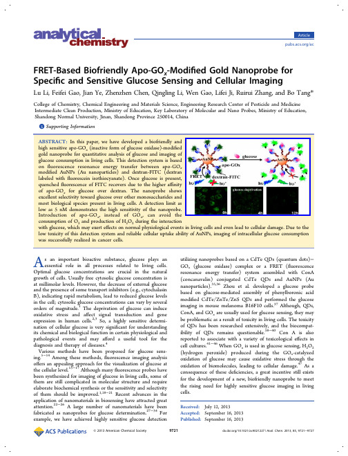
ABSTRACT: In this paper, we have developed a biofriendly and high sensitive apo-GOx (inactive form of glucose oxidase)-modiﬁed gold nanoprobe for quantitative analysis of glucose and imaging of glucose consumption in living cells. This detection system is based on ﬂuorescence resonance energy transfer between apo-GOx modiﬁed AuNPs (Au nanoparticles) and dextran-FITC (dextran labeled with ﬂuorescein isothiocyanate). Once glucose is present, quenched ﬂuorescence of FITC recovers due to the higher aﬃnity of apo-GOx for glucose over dextran. The nanoprobe shows excellent selectivity toward glucose over other monosaccharides and most biological species present in living cells. A detection limit as low as 5 nM demonstrates the high sensitivity of the nanoprobe. Introduction of apo-GOx, instead of GOx, can avoid the consumption of O2 and production of H2O2 during the interaction with glucose, which may exert eﬀects on normal physiological events in living cells and even lead to cellular damage. Due to the low toxicity of this detection system and reliable cellular uptake ability of AuNPs, imaging of intracellular glucose consumption was successfully realized in cancer cells.

Reflection Detection in Image Sequences

Reﬂection Detection in Image SequencesMohamed Abdelaziz Ahmed Francois Pitie Anil KokaramSigmedia,Electronic and Electrical Engineering Department,Trinity College Dublin{/People}AbstractReﬂections in image sequences consist of several layers superimposed over each other.This phenomenon causes many image processing techniques to fail as they assume the presence of only one layer at each examined site e.g.motion estimation and object recognition.This work presents an automated technique for detecting reﬂections in image se-quences by analyzing motion trajectories of feature points. It models reﬂection as regions containing two different lay-ers moving over each other.We present a strong detector based on combining a set of weak detectors.We use novel priors,generate sparse and dense detection maps and our results show high detection rate with rejection to patholog-ical motion and occlusion.1.IntroductionReﬂections are often the result of superimposing differ-ent layers over each other(see Fig.1,2,4,5).They mainly occur due to photographing objects situated behind a semi reﬂective medium(e.g.a glass window).As a result the captured image is a mixture between the reﬂecting surface (background layer)and the reﬂected image(foreground). When viewed from a moving camera,two different layers moving over each other in different directions are observed. This phenomenon violates many of the existing models for video sequences and hence causes many consumer video applications to fail e.g.slow-motion effects,motion based sports summarization and so on.This calls for the need of an automated technique that detects reﬂections and assigns a different treatment to them.Detecting reﬂections requires analyzing data for speciﬁc reﬂection characteristics.However,as reﬂections can arise by mixing any two images,they come in many shapes and colors(Fig.1,2,4,5).This makes extracting characteris-tics speciﬁc to reﬂections not an easy task.Furthermore, one should be careful when using motion information of re-ﬂections as there is a high probability of motion estimation failure.For these reasons the problem of reﬂection detec-tion is hard and was not examined before.Reﬂection can be detected by examining the possibility of decomposing an image into two different layers.Lots of work exist on separating mixtures of semi-transparent lay-ers[17,11,12,7,4,1,13,3,2].Nevertheless,most of the still image techniques[11,4,1,3,2]require two mixtures of the same layers under two different mixing conditions while video techniques[17,12,13]assume a simple rigid motion for the background[17,13]or a repetitive one[12].These assumptions are hardly valid for reﬂections on mov-ing image sequences.This paper presents an automated technique for detect-ing reﬂections in image sequences.It is based on analyzing spatio-temporal proﬁles of feature point trajectories.This work focuses on analyzing three main features of reﬂec-tions:1)the ability of decomposing an image into two in-dependent layers2)image sharpness3)the temporal be-havior of image patches.Several weak detectors based on analyzing these features through different measures are pro-posed.Aﬁnal strong detector is generated by combining the weak detectors.The problem is formulated within a Bayesian framework and priors are deﬁned in a way to re-ject false alarms.Several sequences are processed and re-sults show high detection rate with rejection to complicated motion patterns e.g.blur,occlusion,fast motion.Aspects of novelty in this paper include:1)A technique for decomposing a color still image containing reﬂection into two images containing the structures of the source lay-ers.We do not claim that this technique could be used to fully remove reﬂections from videos.What we claim is that the extracted layers can be useful for reﬂection detection since on a block basis,reﬂection is reduced.This technique can not compete with state of the art separation techniques.However we use this technique because it works on single frames and thus does not require motion,which is not the case with any existing separation technique.2)Diagnos-tic tools for reﬂection detection based on analyzing feature points trajectories3)A scheme for combining weak de-tectors in one strong reﬂection detector using Adaboost4) Incorporating priors which reject spatially and temporally impulsive detections5)The generation of dense detection maps from sparse detections and using thresholding by hys-1Figure1.Examples of different reﬂections(shown in green).Reﬂection is the result of superimposing different layers over each other.As a result they have a wide range of colors and shapes.teresis to avoid selecting particular thresholds for the systemparameters6)Using the generated maps to perform betterframe rate conversion in regions of reﬂection.Frame rateconversion is a computer vision application that is widelyused in the post-production industry.In the next section wepresent a review on the relevant techniques for layer separa-tion.In section3we propose our layer separation technique.We then go to propose our Bayesian framework followed bythe results section.2.Review on Layer Separation TechniquesA mixed image M is modeled as a linear combinationbetween the source layers L1and L2according to the mix-ing parameters(a,b)as follows.M=aL1+bL2(1)Layer separation techniques attempt to decompose reﬂec-tion M into two independent layers.They do so by ex-changing information between the source layers(L1andL2)until their mutual independence is maximized.Thishowever requires the presence of two mixtures of the samelayers under two different mixing proportions[11,4,1,3,2].Different separation techniques use different forms ofexpressing the mutual layer independence.Current formsused include minimizing the number of corners in the sep-arated layers[7]and minimizing the grayscale correlationbetween the layers[11].Other techniques[17,12,13]avoid the requirement ofhaving two mixtures of the same layers by using tempo-ral information.However they often require either a staticbackground throughout the whole image sequence[17],constraint both layers to be of non-varying content throughtime[13],or require the presence of repetitive dynamic mo-tion in one of the layers[12].Yair Weiss[17]developed atechnique which estimates the intrinsic image(static back-ground)of an image sequence.Gradients of the intrinsiclayer are calculated by temporallyﬁltering the gradientﬁeldof the sequence.Filtering is performed in horizontal andvertical directions and the generated gradients are used toreconstruct the rest of the background image.yer Separation Using Color IndependenceThe source layers of a reﬂection M are usually color in-dependent.We noticed that the red and blue channels ofM are the two most uncorrelated RGB channels.Each ofthese channels is usually dominated by one layer.Hence thesource layers(L1,L2)can be estimated by exchanging in-formation between the red and blue channels till the mutualindependence between both channels is r-mation exchange for layer separation wasﬁrst introducedby Sarel et.al[12]and it is reformulated for our problem asfollowsL1=M R−αM BL2=M B−βM R(2)Here(M R,M B)are the red and blue channels of themixture M while(α,β)are separation parameters to becalculated.An exhaustive search for(α,β)is performed.Motivated by Levin et.al.work on layer separation[7],thebest separated layer is selected as the one with the lowestcornerness value.The Harris cornerness operator is usedhere.A minimum texture is imposed on the separated lay-ers by discarding layers with a variance less than T x.For an8-bit image,T x is set to2.The removal of this constraintcan generate empty meaningless layers.The novelty in thislayer separation technique is that unlike previous techniques[11,4,1,3,2],it only requires one image.Fig.2shows separation results generated by the proposedtechnique for different images.Results show that our tech-nique reduces reﬂections and shadows.Results are only dis-played to illustrate a preprocess step,that is used for one ofour reﬂection measures and not to illustrate full reﬂectionremoval.Blocky artifacts are due to processing images in50×50blocks.These artifacts are irrelevant to reﬂectiondetection.4.Bayesian Inference for Reﬂection Detection(BIRD)The goal of the algorithm is toﬁnd regions in imagesequences containing reﬂections.This is achieved by an-(a)(b)(c)(d)(e)(f)Figure 2.Reducing reﬂections/shadows using the proposed layer separation technique.Color images are the original images with reﬂec-tions/shadows (shown in green).The uncolored images represent one source layer (calculated by our technique)with reﬂections/shadows reduced.In (e)reﬂection still remains apparent however the person in the car is fully removed.alyzing trajectories of feature points.Trajectories are gen-erated using KLT feature point tracker [9,14].Denote P inas the feature point of i th track in frame n and F inas the 50×50image patch centered on P in .Trajectories are ana-lyzed by examining all feature points along tracks of length more than 4frames.For each point,analysis are carriedover the three image patches (F i n −1,F i n ,F in +1).Based onthe analysis outcome,a binary label ﬁeld l in is assigned toeach F i n .l in is set to 1for reﬂection and 0otherwise.4.1.Bayesian FrameworkThe system derives an estimate for l in from the posterior P (l |F )(where (i,n)are dropped for clarity).The posterior is factorized in a Bayesian fashion as followsP (l |F )=P (F|l )P (l |l N )(3)The likelihood term P (F|l )consists of 9detectors D 1−D 9each performing different analysis on F and operating at thresholds T 1−9(see Sec.4.5.1).The prior P (l |l N )en-forces various smoothness constraints in space and time toreject spatially and temporally impulsive detections and to generate dense detection masks.Here N denote the spatio-temporal neighborhood of the examined site.yer Separation LikelihoodThis likelihood measures the ability of decomposing animage patch F in into two independent layers.Three detec-tors are proposed.Two of them attempts to perform layer separation before analyzing data while the third measures the possibility of layer separation by measuring the color channels independence.Layer Separation via Color Independence D 1:Our technique (presented in Sec.3)is used to decompose the im-age patch F i n into two layers L 1i n and L 2in .This is applied for every point along every track.Reﬂection is detected by comparing the temporal behavior of the observed image patches F with the temporal behavior of the extracted lay-ers.Patches containing reﬂection are deﬁned as ones with higher temporal discontinuity before separation than after separation.Temporal discontinuity is measured using struc-ture similarity index SSIM[16]as followsD1i n=max(SS(G i n,G i n−1),SS(G i n,G i n+1))−max(SS(L i n,L i n−1),SS(L i n,L i n+1))SS(L i n,L i n−1)=max(SS(L1i n,L1i n−1),SS(L2i n,L2i n−1))) SS(L i n,L i n+1)=max(SS(L1i n,L1i n+1),SS(L2i n,L2i n+1)) Here G=0.1F R+0.7F G+0.2F B where(F R,F G,F B) are the red,green and blue components of F respectively. SS(G i n,G i n−1)denotes the structure similarity between the two images F i n and F i n−1.We only compare the structures of(G i n,G i n−1)by turning off the luminance component of SSIM[16].SS(.,.)returns an a value between0−1where 1denotes identical similarity.Reﬂection is detected if D1i n is less than T1.Intrinsic Layer Extraction D2:Let INTR i denote the intrinsic(reﬂectance)image extracted by processing the 50×50i th track using Yair technique[17].In case of re-ﬂection the structure similarity between the observed mix-ture F i n and INTR i should be low.Therefore,F i n isﬂagged as containing reﬂection if SS(F i n,INTR i)is less than T2.Color Channels Independence D3:This approach measures the Generalized Normalized Cross Correlation (GNGC)[11]between the red and blue channels of the ex-amined patch F i n to infer whether the patch is a mixture between two different layers or not.GNGC takes values between0and1where1denotes perfect match between the red and blue channels(M R and M B respectively).This analysis is applied to every image patch F i n and reﬂection is detected if GNGC(M R,M B)<T3.4.3.Image Sharpness Likelihood:D4,D5Two approaches for analyzing image sharpness are used. Theﬁrst,D4,estimates theﬁrst order derivatives for the examined patch F i n andﬂags it as containing reﬂection if the mean of the gradient magnitude within the examined patch is smaller than a threshold T4.The second approach, D5,uses the sharpness metric of Ferzil et.al.[5]andﬂagsa patch as reﬂection if its sharpness value is less than T5.4.4.Temporal Discontinuity LikelihoodSIFT Temporal Proﬁle D6:This detectorﬂags the ex-amined patch F i n as reﬂection if its SIFT features[8]are undergoing high temporal mismatch.A vector p=[x s g]is assigned to every interest point in F i n.The vector contains the position of the point x=(x,y),scale and dominate ori-entation from the SIFT descriptor,s=(δ,o),and the128 point SIFT descriptor g.Interest points are matched with neighboring frames using[8].F i n isﬂagged as reﬂection if the average distance between the matched vectors p is larger than T6.Color Temporal Proﬁle D7:This detectorﬂags the im-age patch F i n as reﬂection if its grayscale proﬁle does not change smoothly through time.The temporal change in color is deﬁned as followsD7i n=min( C i n−C i n−1 , C i n−C i n+1 )(4) Here C i n is the mean value for G i n,the grayscale representa-tion of F i n.F i n isﬂagged as reﬂection if D7i n>T7.AutoCorrelation Temporal Proﬁle D8:This detector ﬂags the image patch F i n as reﬂection if its autocorrelation is undergoing large temporal change.The temporal change in the autocorrelation is deﬁned as followsD8i n=min(1NA i n−A i n−1 2,1NA i n−A i n+1 2)(5)A i n is a vector containing the autocorrelation of G i n while N is the number of pels in A i n.F i n isﬂagged as reﬂection if D8i n is bigger than T8.Motion Field Divergence D9:D9for the examined patch F i n is deﬁned as followsD9i n=DFD( div(d(n)) + div(d(n+1)) )/2(6) DFD and div(d(n))are the Displaced Frame Difference and Motion Field Divergence for F i n.d(n)is the2D motion vector calculated using block matching.DFD is set to the minimum of the forward and backward DFDs.div(d(n)) is set to the minimum of the forward and backward di-vergence.The divergence is averaged over blocks of two frames to reduce the effect of possible motion blur gener-ated by unsteady camera motion.F i n isﬂagged as reﬂection if D9>T9.4.5.Solving for l in4.5.1Maximum Likelihood(ML)SolutionThe likelihood is factorized as followsP(F|l)=P(l|D1)P(l|D2−8)P(l|D9)(7)Theﬁrst and last terms are solved using D1<T1and D9>T9respectively.D2−8are used to form one strong detector D s and P(l|D2−8)is solved by D s>T s.We found that not including(D1,D9)in D s generates better de-tection results than when included.Feature analysis of each detector are averaged over a block of three frames to gen-erate temporally consistent detections.T9isﬁxed to10in all experiments.In Sec.4.5.2we avoid selecting particular thresholds for(T1,T s)by imposing spatial and temporal priors on the generated maps.Calculating D s:The strong detector D s is expressed as a linear combination of weak detectors operating at different thresholds T as followsP(l|D2−8)=Mk=1W(V(k),T)P(D V(k)|T)(8)False Alarm RateC o r r e c tD e t e c t i o n R a t eFigure 3.ROC for D 1−9and D s .The Adaboost detector D s out-performs all other techniques and D 1is the second best in the range of false alarms <0.1.Here M is the number of weak detectors (ﬁxed to 20)used in forming D s and V (k )is a function which returns a value between 2-8to indicate which detectors from D 2−8are used.k indexes the weak detectors in order of their impor-tance as deﬁned by the weights W .W and T are learned through Adaboost [15](see Tab.1).Our training set consist of 89393images of size 50×50pels.Reﬂection is modeled in 35966images each being a synthetic mixture between two different images.Fig.3shows the the Receiver Operating Characteristic (ROC)of applying D 1−9and D s on the training samples.D s outperforms all the other detectors due to its higher cor-rect detection rate and lower false alarms.D 6D 8D 5D 3D 2D 4D 7W 1.310.960.480.520.330.320.26T0.296.76e −60.040.950.6172.17Table 1.Weights W and operating thresholds T for the best seven detectors selected by Adaboost.4.5.2Successive Reﬁnement for Maximum A-Posteriori (MAP)The prior P (l |l N )of Eq.3imposes spatial and temporal smoothness on detection masks.We create a MAP estimate by reﬁning the sparse maps from the previous ML steps.We ﬁrst reﬁne the labeling of all the existing feature points P in each image and then use the overlapping 50×50patches around the reﬁned labeled points as a dense pixel map.ML Reﬁnement:First we reject false detections from ML which are spatially inconsistent.Every feature point l =1is considered and the sum of the geodesic distance from that site to the two closest neighbors which are labeledl =1is measured.When that distance is more than 0.005then that decision is rejected i.e.we set l =0.Geodesic distances allow the nature of the image material between point to be taken in to account more effectively and have been in use for some time now [10].To reduce the compu-tational load of this step,we downsample the image mas-sively by 50in both directions.This retains gross image topology only.Spatio-Temporal Dilation:Labels are extended in space and time to other feature points along their trajecto-ries.If l in =1,all feature points lying along the track i are set to l =1.In addition,l is extended to all image patches (F n )overlapping spatially with the examined patch.This generates a denser representation of the detection masks.We call this step ML-Denser.Hysteresis:We can avoid selecting particular thresholds [T 1,T s ]for BIRD by applying Hysteresis using a set of dif-ferent thresholds.Let T H =[−0.4,5]and T L =[0,3]de-note a high and low conﬁguration for [T 1,T s ].Detection starts by examining ML-Denser at high thresholds.High thresholds generate detected points P h with high conﬁ-dence.Points within a small geodesic distance (<D geo )and small euclidean distance (<D euc )to each other are grouped together.Here we use (D geo ,D euc )=(0.0025,4)and resize the examined frames as mentioned previously.The centroids of each group is then calculated.Thresholds are lowered and a new detection point is added to an exist-ing group if it is within D geo and D euc to the centroid of this group.This is the hysteresis idea.If however the examined point has a large euclidean distance (>D euc )but a small geodesic distance (<D geo )to the centroid of all existing groups,a new group is formed.Points at which distances >D geo and >D euc are regarded as outliers and discarded.Group centroids are updated and the whole process is re-peated iteratively till the examined threshold reaches T L .The detection map generated at T L is made more dense by performing Spatio-Temporal Dilation above.Spatio-Temporal ‘Opening’:False alarms of the previ-ous step are removed by propagating the patches detected in the ﬁrst frame to the rest of the sequence along the fea-ture point trajectories.A detection sample at fame n is kept if it agrees with the propagated detections from the previous frame.Correct detections missed from this step are recovered by running Spatio-Temporal Dilation on the ‘temporally eroded’solution.This does mean that trajecto-ries which do not start in the ﬁrst frame are not likely to be considered,however this does not affect the performance in our real examples shown here.The selection of an optimal frame from which to perform this opening operation is the subject of future work.=Figure 4.From Top:ML (calculated at (T 1,T s )=(−0.13,3.15)),Hysteresis and Spatio-Temporal ‘Opening’for three consecutive frames from the SelimH sequence.Reﬂection is shown in red and detected reﬂection using our technique is shown in green.Spatio-Temporal ‘Opening’rejects false alarms generated by ML and by Hysteresis (shown in yellow and blue respectively).5.Results5.1.Reﬂection Detection15sequences containing 932frames of size 576×720are processed with BIRD.Full sequences with reﬂection de-tection can be found in /Misc/CVPR2011.Fig.4compares the ML,Hysteresis and Spatio-Temporal ‘Opening’for three consecutive frames from the SelimH se-quence.This sequence contains occlusion,motion blur and strong edges in the reﬂection (shown in red).The ML so-lution (ﬁrst line)generates good sparse reﬂection detection (shown in green),however it generates some errors (shown in yellow).Hysteresis rejects these errors and generates dense masks with some false alarm (shown in blue).These false alarms are rejected by Spatio-Temporal ‘Opening’.Fig.5shows the result of processing four sequences us-ing BIRD.In the ﬁrst two sequences,BIRD detected regions of reﬂections correctly and discarded regions of occlusion (shown in purple)and motion blur (shown in blue).In Girl-Ref most of the sequence is correctly classiﬁed as reﬂection.In SelimK1the portrait on the right is correctly classiﬁed as containing reﬂection even in the presence of motion blur (shown in blue).Nevertheless,BIRD failed in detecting the reﬂection on the left portrait as it does not contain strong distinctive feature points.Fig.6shows the ROC plot for 50frames from SelimH .Here we compare our technique BIRD against DFD and Im-age Sharpness[5].DFD,ﬂags a region as reﬂection if it has high displaced frame difference.Image Sharpness ﬂags a region as reﬂection if it has low sharpness.Frames are pro-cessed on 50×50blocks.Ground truth reﬂection masks are generated manually and detection rates are calculated on pel basis.The ROC shows that BIRD outperforms the other techniques by achieving a very high correct detection rate of 0.9for a false detection rate of 0.1.This is a major improvement over a correct detection rate of 0.2and 0.1for DFD and Sharpness respectively.5.2.Frame Rate Conversion:An applicationOne application for reﬂection detection is improving frame rate conversion in regions of reﬂection.Frame rate conversion is the process of creating new frames from ex-isting ones.This is done by using motion vectors to inter-polate objects in the new frames.This process usually fails in regions of reﬂection due to motion estimation failure.Fig.7illustrates the generation of a slow motion effect for the person’s leg in GirlRef (see Fig.5,third line).This is done by doubling the frame rate using the Foundry’s Kro-nos plugin [6].Kronos has an input which deﬁnes the den-sity of the motion vector ﬁeld.The larger the density theFigure 5.Detection results of BIRD (shown in green)on,From top:BuilOnWind [10,35,49],PHouse 9-11,GirlRef [45,55,65],SelimK132-35.Reﬂections are shown in red.Good detections are generated despite occlusion (shown in purple)and motion blur (shown in blue).For GirlRef we replace Hysteresis and Spatio-Temporal ‘Opening’with a manual parameter conﬁguration of (T 1,T s )=(−0.01,3.15)followed by a Spatio-Temporal Dilation step.This setting generates good detections for all examined sequences with static backgrounds.more detailed the vector and hence the better the interpo-lation.However,using highly detailed vectors generate ar-tifacts in regions of reﬂections as shown in Fig.7(second line).We reduce these artifacts by lowering the motion vec-tor density in regions of reﬂection indicated by BIRD (see Fig.7,third line).Image sequence results and more exam-ples are available in /Misc/CVPR2011.6.ConclusionThis paper has presented a technique for detecting reﬂec-tions in image sequences.This problem was not addressed before.Our technique performs several analysis on feature point trajectories and generates a strong detector by com-bining these analysis.Results show major improvement over techniques which measure image sharpness and tem-poral discontinuity.Our technique generates high correct detection rate with rejection to regions containing compli-cated motion eg.motion blur,occlusion.The technique was fully automated in generating most results.As an ap-plication,we showed how the generated detections can be used to improve frame rate conversion.A limiting factor of our technique is that it requires source layers with strong distinctive feature points.This could lead to incomplete de-tections.Acknowledgment:This work is funded by the Irish Re-serach Council for Science,Engineering and TechnologyFigure 7.Slow motion effect for the person’s leg of GirlRef (see Fig:5third line).Top:Original frames 59-61;Middle:generated frames using the Foundry’s plugin Kronos [6]with one motion vector calculated for every 4pels;Bottom;with one motion vector calculated for every 64pels in regions of reﬂection.False Alarm RateC o r r e c tD e t e c t i o n R a t eFigure 6.ROC plots for our technique BIRD,DFD and Sharpness for SelimH .Our technique BIRD outperforms DFD and Sharp-ness with a massive increase in the Correct Detection Rate.(IRCSET)and Science Foundation Ireland (SFI).References[1] A.M.Bronstein,M.M.Bronstein,M.Zibulevsky,and Y .Y .Zeevi.Sparse ICA for blind separation of transmitted and reﬂected images.International Journal of Imaging Systems and Technology ,15(1):84–91,2005.1,2[2]N.Chen and P.De Leon.Blind image separation throughkurtosis maximization.In Asilomar Conference on Signals,Systems and Computers ,volume 1,pages 318–322,2001.1,2[3]K.Diamantaras and T.Papadimitriou.Blind separation ofreﬂections using the image mixtures ratio.In ICIP ,pages 1034–1037,2005.1,2[4]H.Farid and E.Adelson.Separating reﬂections from imagesby use of independent components analysis.Journal of the Optical Society of America ,16(9):2136–2145,1999.1,2[5]R.Ferzli and L.J.Karam.A no-reference objective imagesharpness metric based on the notion of just noticeable blur (jnb).IEEE Trans.on Img.Proc.(TIPS),18(4):717–728,2009.4,6[6]T.Foundry.Nuke,furnace .6,8[7] A.Levin,A.Zomet,and Y .Weiss.Separating reﬂectionsfrom a single image using local features.In IEEE Conference on Computer Vision and Pattern Recognition (CVPR),pages 306–313,2004.1,2[8] D.G.Lowe.Distinctive image features from scale-invariantput.Vision ,60(2):91–110,2004.4[9] B.D.Lucas and T.Kanade.An iterative image registra-tion technique with an application to stereo vision (darpa).In DARPA Image Understanding Workshop ,pages 121–130,1981.3[10] D.Ring and F.Pitie.Feature-assisted sparse to dense motionestimation using geodesic distances.In International Ma-chine Vision and Image Processing Conference ,pages 7–12,2009.5[11] B.Sarel and M.Irani.Separating transparent layers throughlayer information exchange.In European Conference on Computer Vision (ECCV),pages 328–341,2004.1,2,4[12] B.Sarel and M.Irani.Separating transparent layers of repet-itive dynamic behaviors.In ICCV ,pages 26–32,2005.1,2[13]R.Szeliski,S.Avidan,and yer extrac-tion from multiple images containing reﬂections and trans-parency.In CVPR ,volume 1,pages 246–253,2000.1,2[14] C.T.Takeo and T.Kanade.Detection and tracking ofpoint features.Carnegie Mellon University Technical Report CMU-CS-91-132,1991.3[15]P.Viola and M.Jones.Robust real-time object detection.InInternational Journal of Computer Vision ,2001.5[16]Z.Wang,A.Bovik,H.Sheikh,and E.Simoncelli.Imagequality assessment:from error visibility to structural simi-larity.TIPS ,13(4):600–612,April 2004.4[17]Y .Weiss.Deriving intrinsic images from image sequences.In ICCV ,pages 68–75,2001.1,2,4。

毕业设计论文塑料注射成型

Modeling of morphology evolution in the injection moldingprocess of thermoplastic polymersR.Pantani,I.Coccorullo,V.Speranza,G.Titomanlio* Department of Chemical and Food Engineering,University of Salerno,via Ponte don Melillo,I-84084Fisciano(Salerno),Italy Received13May2005;received in revised form30August2005;accepted12September2005AbstractA thorough analysis of the effect of operative conditions of injection molding process on the morphology distribution inside the obtained moldings is performed,with particular reference to semi-crystalline polymers.The paper is divided into two parts:in the ﬁrst part,the state of the art on the subject is outlined and discussed;in the second part,an example of the characterization required for a satisfactorily understanding and description of the phenomena is presented,starting from material characterization,passing through the monitoring of the process cycle and arriving to a deep analysis of morphology distribution inside the moldings.In particular,fully characterized injection molding tests are presented using an isotactic polypropylene,previously carefully characterized as far as most of properties of interest.The effects of both injectionﬂow rate and mold temperature are analyzed.The resulting moldings morphology(in terms of distribution of crystallinity degree,molecular orientation and crystals structure and dimensions)are analyzed by adopting different experimental techniques(optical,electronic and atomic force microscopy,IR and WAXS analysis).Final morphological characteristics of the samples are compared with the predictions of a simulation code developed at University of Salerno for the simulation of the injection molding process.q2005Elsevier Ltd.All rights reserved.Keywords:Injection molding;Crystallization kinetics;Morphology;Modeling;Isotactic polypropyleneContents1.Introduction (1186)1.1.Morphology distribution in injection molded iPP parts:state of the art (1189)1.1.1.Modeling of the injection molding process (1190)1.1.2.Modeling of the crystallization kinetics (1190)1.1.3.Modeling of the morphology evolution (1191)1.1.4.Modeling of the effect of crystallinity on rheology (1192)1.1.5.Modeling of the molecular orientation (1193)1.1.6.Modeling of theﬂow-induced crystallization (1195)ments on the state of the art (1197)2.Material and characterization (1198)2.1.PVT description (1198)*Corresponding author.Tel.:C39089964152;fax:C39089964057.E-mail address:gtitomanlio@unisa.it(G.Titomanlio).2.2.Quiescent crystallization kinetics (1198)2.3.Viscosity (1199)2.4.Viscoelastic behavior (1200)3.Injection molding tests and analysis of the moldings (1200)3.1.Injection molding tests and sample preparation (1200)3.2.Microscopy (1202)3.2.1.Optical microscopy (1202)3.2.2.SEM and AFM analysis (1202)3.3.Distribution of crystallinity (1202)3.3.1.IR analysis (1202)3.3.2.X-ray analysis (1203)3.4.Distribution of molecular orientation (1203)4.Analysis of experimental results (1203)4.1.Injection molding tests (1203)4.2.Morphology distribution along thickness direction (1204)4.2.1.Optical microscopy (1204)4.2.2.SEM and AFM analysis (1204)4.3.Morphology distribution alongﬂow direction (1208)4.4.Distribution of crystallinity (1210)4.4.1.Distribution of crystallinity along thickness direction (1210)4.4.2.Crystallinity distribution alongﬂow direction (1212)4.5.Distribution of molecular orientation (1212)4.5.1.Orientation along thickness direction (1212)4.5.2.Orientation alongﬂow direction (1213)4.5.3.Direction of orientation (1214)5.Simulation (1214)5.1.Pressure curves (1215)5.2.Morphology distribution (1215)5.3.Molecular orientation (1216)5.3.1.Molecular orientation distribution along thickness direction (1216)5.3.2.Molecular orientation distribution alongﬂow direction (1216)5.3.3.Direction of orientation (1217)5.4.Crystallinity distribution (1217)6.Conclusions (1217)References (1219)1.IntroductionInjection molding is one of the most widely employed methods for manufacturing polymeric products.Three main steps are recognized in the molding:ﬁlling,packing/holding and cooling.During theﬁlling stage,a hot polymer melt rapidlyﬁlls a cold mold reproducing a cavity of the desired product shape. During the packing/holding stage,the pressure is raised and extra material is forced into the mold to compensate for the effects that both temperature decrease and crystallinity development determine on density during solidiﬁcation.The cooling stage starts at the solidiﬁcation of a thin section at cavity entrance (gate),starting from that instant no more material can enter or exit from the mold impression and holding pressure can be released.When the solid layer on the mold surface reaches a thickness sufﬁcient to assure required rigidity,the product is ejected from the mold.Due to the thermomechanical history experienced by the polymer during processing,macromolecules in injection-molded objects present a local order.This order is referred to as‘morphology’which literally means‘the study of the form’where form stands for the shape and arrangement of parts of the object.When referred to polymers,the word morphology is adopted to indicate:–crystallinity,which is the relative volume occupied by each of the crystalline phases,including mesophases;–dimensions,shape,distribution and orientation of the crystallites;–orientation of amorphous phase.R.Pantani et al./Prog.Polym.Sci.30(2005)1185–1222 1186R.Pantani et al./Prog.Polym.Sci.30(2005)1185–12221187Apart from the scientiﬁc interest in understandingthe mechanisms leading to different order levels inside a polymer,the great technological importance of morphology relies on the fact that polymer character-istics (above all mechanical,but also optical,electrical,transport and chemical)are to a great extent affected by morphology.For instance,crystallinity has a pro-nounced effect on the mechanical properties of the bulk material since crystals are generally stiffer than amorphous material,and also orientation induces anisotropy and other changes in mechanical properties.In this work,a thorough analysis of the effect of injection molding operative conditions on morphology distribution in moldings with particular reference to crystalline materials is performed.The aim of the paper is twofold:ﬁrst,to outline the state of the art on the subject;second,to present an example of the characterization required for asatisfactorilyR.Pantani et al./Prog.Polym.Sci.30(2005)1185–12221188understanding and description of the phenomena, starting from material description,passing through the monitoring of the process cycle and arriving to a deep analysis of morphology distribution inside the mold-ings.To these purposes,fully characterized injection molding tests were performed using an isotactic polypropylene,previously carefully characterized as far as most of properties of interest,in particular quiescent nucleation density,spherulitic growth rate and rheological properties(viscosity and relaxation time)were determined.The resulting moldings mor-phology(in terms of distribution of crystallinity degree, molecular orientation and crystals structure and dimensions)was analyzed by adopting different experimental techniques(optical,electronic and atomic force microscopy,IR and WAXS analysis).Final morphological characteristics of the samples were compared with the predictions of a simulation code developed at University of Salerno for the simulation of the injection molding process.The effects of both injectionﬂow rate and mold temperature were analyzed.1.1.Morphology distribution in injection molded iPP parts:state of the artFrom many experimental observations,it is shown that a highly oriented lamellar crystallite microstructure, usually referred to as‘skin layer’forms close to the surface of injection molded articles of semi-crystalline polymers.Far from the wall,the melt is allowed to crystallize three dimensionally to form spherulitic structures.Relative dimensions and morphology of both skin and core layers are dependent on local thermo-mechanical history,which is characterized on the surface by high stress levels,decreasing to very small values toward the core region.As a result,the skin and the core reveal distinct characteristics across the thickness and also along theﬂow path[1].Structural and morphological characterization of the injection molded polypropylene has attracted the interest of researchers in the past three decades.In the early seventies,Kantz et al.[2]studied the morphology of injection molded iPP tensile bars by using optical microscopy and X-ray diffraction.The microscopic results revealed the presence of three distinct crystalline zones on the cross-section:a highly oriented non-spherulitic skin;a shear zone with molecular chains oriented essentially parallel to the injection direction;a spherulitic core with essentially no preferred orientation.The X-ray diffraction studies indicated that the skin layer contains biaxially oriented crystallites due to the biaxial extensionalﬂow at theﬂow front.A similar multilayered morphology was also reported by Menges et al.[3].Later on,Fujiyama et al.[4] investigated the skin–core morphology of injection molded iPP samples using X-ray Small and Wide Angle Scattering techniques,and suggested that the shear region contains shish–kebab structures.The same shish–kebab structure was observed by Wenig and Herzog in the shear region of their molded samples[5].A similar investigation was conducted by Titomanlio and co-workers[6],who analyzed the morphology distribution in injection moldings of iPP. They observed a skin–core morphology distribution with an isotropic spherulitic core,a skin layer characterized by aﬁne crystalline structure and an intermediate layer appearing as a dark band in crossed polarized light,this layer being characterized by high crystallinity.Kalay and Bevis[7]pointed out that,although iPP crystallizes essentially in the a-form,a small amount of b-form can be found in the skin layer and in the shear region.The amount of b-form was found to increase by effect of high shear rates[8].A wide analysis on the effect of processing conditions on the morphology of injection molded iPP was conducted by Viana et al.[9]and,more recently, by Mendoza et al.[10].In particular,Mendoza et al. report that the highest level of crystallinity orientation is found inside the shear zone and that a high level of orientation was also found in the skin layer,with an orientation angle tilted toward the core.It is rather difﬁcult to theoretically establish the relationship between the observed microstructure and processing conditions.Indeed,a model of the injection molding process able to predict morphology distribution in theﬁnal samples is not yet available,even if it would be of enormous strategic importance.This is mainly because a complete understanding of crystallization kinetics in processing conditions(high cooling rates and pressures,strong and complexﬂowﬁelds)has not yet been reached.In this section,the most relevant aspects for process modeling and morphology development are identiﬁed. In particular,a successful path leading to a reliable description of morphology evolution during polymer processing should necessarily pass through:–a good description of morphology evolution under quiescent conditions(accounting all competing crystallization processes),including the range of cooling rates characteristic of processing operations (from1to10008C/s);R.Pantani et al./Prog.Polym.Sci.30(2005)1185–12221189–a description capturing the main features of melt morphology(orientation and stretch)evolution under processing conditions;–a good coupling of the two(quiescent crystallization and orientation)in order to capture the effect of crystallinity on viscosity and the effect ofﬂow on crystallization kinetics.The points listed above outline the strategy to be followed in order to achieve the basic understanding for a satisfactory description of morphology evolution during all polymer processing operations.In the following,the state of art for each of those points will be analyzed in a dedicated section.1.1.1.Modeling of the injection molding processTheﬁrst step in the prediction of the morphology distribution within injection moldings is obviously the thermo-mechanical simulation of the process.Much of the efforts in the past were focused on the prediction of pressure and temperature evolution during the process and on the prediction of the melt front advancement [11–15].The simulation of injection molding involves the simultaneous solution of the mass,energy and momentum balance equations.Theﬂuid is non-New-tonian(and viscoelastic)with all parameters dependent upon temperature,pressure,crystallinity,which are all function of pressibility cannot be neglected as theﬂow during the packing/holding step is determined by density changes due to temperature, pressure and crystallinity evolution.Indeed,apart from some attempts to introduce a full 3D approach[16–19],the analysis is currently still often restricted to the Hele–Shaw(or thinﬁlm) approximation,which is warranted by the fact that most injection molded parts have the characteristic of being thin.Furthermore,it is recognized that the viscoelastic behavior of the polymer only marginally inﬂuences theﬂow kinematics[20–22]thus the melt is normally considered as a non-Newtonian viscousﬂuid for the description of pressure and velocity gradients evolution.Some examples of adopting a viscoelastic constitutive equation in the momentum balance equations are found in the literature[23],but the improvements in accuracy do not justify a considerable extension of computational effort.It has to be mentioned that the analysis of some features of kinematics and temperature gradients affecting the description of morphology need a more accurate description with respect to the analysis of pressure distributions.Some aspects of the process which were often neglected and may have a critical importance are the description of the heat transfer at polymer–mold interface[24–26]and of the effect of mold deformation[24,27,28].Another aspect of particular interest to the develop-ment of morphology is the fountainﬂow[29–32], which is often neglected being restricted to a rather small region at theﬂow front and close to the mold walls.1.1.2.Modeling of the crystallization kineticsIt is obvious that the description of crystallization kinetics is necessary if theﬁnal morphology of the molded object wants to be described.Also,the development of a crystalline degree during the process inﬂuences the evolution of all material properties like density and,above all,viscosity(see below).Further-more,crystallization kinetics enters explicitly in the generation term of the energy balance,through the latent heat of crystallization[26,33].It is therefore clear that the crystallinity degree is not only a result of simulation but also(and above all)a phenomenon to be kept into account in each step of process modeling.In spite of its dramatic inﬂuence on the process,the efforts to simulate the injection molding of semi-crystalline polymers are crude in most of the commercial software for processing simulation and rather scarce in the ﬂeur and Kamal[34],Papatanasiu[35], Titomanlio et al.[15],Han and Wang[36],Ito et al.[37],Manzione[38],Guo and Isayev[26],and Hieber [25]adopted the following equation(Kolmogoroff–Avrami–Evans,KAE)to predict the development of crystallinityd xd tZð1K xÞd d cd t(1)where x is the relative degree of crystallization;d c is the undisturbed volume fraction of the crystals(if no impingement would occur).A signiﬁcant improvement in the prediction of crystallinity development was introduced by Titoman-lio and co-workers[39]who kept into account the possibility of the formation of different crystalline phases.This was done by assuming a parallel of several non-interacting kinetic processes competing for the available amorphous volume.The evolution of each phase can thus be described byd x id tZð1K xÞd d c id t(2)where the subscript i stands for a particular phase,x i is the relative degree of crystallization,x ZPix i and d c iR.Pantani et al./Prog.Polym.Sci.30(2005)1185–1222 1190is the expectancy of volume fraction of each phase if no impingement would occur.Eq.(2)assumes that,for each phase,the probability of the fraction increase of a single crystalline phase is simply the product of the rate of growth of the corresponding undisturbed volume fraction and of the amount of available amorphous fraction.By summing up the phase evolution equations of all phases(Eq.(2))over the index i,and solving the resulting differential equation,one simply obtainsxðtÞZ1K exp½K d cðtÞ (3)where d c Z Pid c i and Eq.(1)is recovered.It was shown by Coccorullo et al.[40]with reference to an iPP,that the description of the kinetic competition between phases is crucial to a reliable prediction of solidiﬁed structures:indeed,it is not possible to describe iPP crystallization kinetics in the range of cooling rates of interest for processing(i.e.up to several hundreds of8C/s)if the mesomorphic phase is neglected:in the cooling rate range10–1008C/s, spherulite crystals in the a-phase are overcome by the formation of the mesophase.Furthermore,it has been found that in some conditions(mainly at pressures higher than100MPa,and low cooling rates),the g-phase can also form[41].In spite of this,the presence of different crystalline phases is usually neglected in the literature,essentially because the range of cooling rates investigated for characterization falls in the DSC range (well lower than typical cooling rates of interest for the process)and only one crystalline phase is formed for iPP at low cooling rates.It has to be noticed that for iPP,which presents a T g well lower than ambient temperature,high values of crystallinity degree are always found in solids which passed through ambient temperature,and the cooling rate can only determine which crystalline phase forms, roughly a-phase at low cooling rates(below about 508C/s)and mesomorphic phase at higher cooling rates.The most widespread approach to the description of kinetic constant is the isokinetic approach introduced by Nakamura et al.According to this model,d c in Eq.(1)is calculated asd cðtÞZ ln2ðt0KðTðsÞÞd s2 435n(4)where K is the kinetic constant and n is the so-called Avrami index.When introduced as in Eq.(4),the reciprocal of the kinetic constant is a characteristic time for crystallization,namely the crystallization half-time, t05.If a polymer is cooled through the crystallization temperature,crystallization takes place at the tempera-ture at which crystallization half-time is of the order of characteristic cooling time t q deﬁned ast q Z D T=q(5) where q is the cooling rate and D T is a temperature interval over which the crystallization kinetic constant changes of at least one order of magnitude.The temperature dependence of the kinetic constant is modeled using some analytical function which,in the simplest approach,is described by a Gaussian shaped curve:KðTÞZ K0exp K4ln2ðT K T maxÞ2D2(6)The following Hoffman–Lauritzen expression[42] is also commonly adopted:K½TðtÞ Z K0exp KUÃR$ðTðtÞK T NÞ!exp KKÃ$ðTðtÞC T mÞ2TðtÞ2$ðT m K TðtÞÞð7ÞBoth equations describe a bell shaped curve with a maximum which for Eq.(6)is located at T Z T max and for Eq.(7)lies at a temperature between T m(the melting temperature)and T N(which is classically assumed to be 308C below the glass transition temperature).Accord-ing to Eq.(7),the kinetic constant is exactly zero at T Z T m and at T Z T N,whereas Eq.(6)describes a reduction of several orders of magnitude when the temperature departs from T max of a value higher than2D.It is worth mentioning that only three parameters are needed for Eq.(6),whereas Eq.(7)needs the deﬁnition ofﬁve parameters.Some authors[43,44]couple the above equations with the so-called‘induction time’,which can be deﬁned as the time the crystallization process starts, when the temperature is below the equilibrium melting temperature.It is normally described as[45]Dt indDtZðT0m K TÞat m(8)where t m,T0m and a are material constants.It should be mentioned that it has been found[46,47]that there is no need to explicitly incorporate an induction time when the modeling is based upon the KAE equation(Eq.(1)).1.1.3.Modeling of the morphology evolutionDespite of the fact that the approaches based on Eq.(4)do represent a signiﬁcant step toward the descriptionR.Pantani et al./Prog.Polym.Sci.30(2005)1185–12221191of morphology,it has often been pointed out in the literature that the isokinetic approach on which Nakamura’s equation (Eq.(4))is based does not describe details of structure formation [48].For instance,the well-known experience that,with many polymers,the number of spherulites in the ﬁnal solid sample increases strongly with increasing cooling rate,is indeed not taken into account by this approach.Furthermore,Eq.(4)describes an increase of crystal-linity (at constant temperature)depending only on the current value of crystallinity degree itself,whereas it is expected that the crystallization rate should depend also on the number of crystalline entities present in the material.These limits are overcome by considering the crystallization phenomenon as the consequence of nucleation and growth.Kolmogoroff’s model [49],which describes crystallinity evolution accounting of the number of nuclei per unit volume and spherulitic growth rate can then be applied.In this case,d c in Eq.(1)is described asd ðt ÞZ C m ðt 0d N ðs Þd s$ðt sG ðu Þd u 2435nd s (9)where C m is a shape factor (C 3Z 4/3p ,for spherical growth),G (T (t ))is the linear growth rate,and N (T (t ))is the nucleation density.The following Hoffman–Lauritzen expression is normally adopted for the growth rateG ½T ðt Þ Z G 0exp KUR $ðT ðt ÞK T N Þ!exp K K g $ðT ðt ÞC T m Þ2T ðt Þ2$ðT m K T ðt ÞÞð10ÞEqs.(7)and (10)have the same form,however the values of the constants are different.The nucleation mechanism can be either homo-geneous or heterogeneous.In the case of heterogeneous nucleation,two equations are reported in the literature,both describing the nucleation density as a function of temperature [37,50]:N ðT ðt ÞÞZ N 0exp ½j $ðT m K T ðt ÞÞ (11)N ðT ðt ÞÞZ N 0exp K 3$T mT ðt ÞðT m K T ðt ÞÞ(12)In the case of homogeneous nucleation,the nucleation rate rather than the nucleation density is function of temperature,and a Hoffman–Lauritzen expression isadoptedd N ðT ðt ÞÞd t Z N 0exp K C 1ðT ðt ÞK T N Þ!exp KC 2$ðT ðt ÞC T m ÞT ðt Þ$ðT m K T ðt ÞÞð13ÞConcentration of nucleating particles is usually quite signiﬁcant in commercial polymers,and thus hetero-geneous nucleation becomes the dominant mechanism.When Kolmogoroff’s approach is followed,the number N a of active nuclei at the end of the crystal-lization process can be calculated as [48]N a ;final Zðt final 0d N ½T ðs Þd sð1K x ðs ÞÞd s (14)and the average dimension of crystalline structures can be attained by geometrical considerations.Pantani et al.[51]and Zuidema et al.[22]exploited this method to describe the distribution of crystallinity and the ﬁnal average radius of the spherulites in injection moldings of polypropylene;in particular,they adopted the following equationR Z ﬃﬃﬃﬃﬃﬃﬃﬃﬃﬃﬃﬃﬃﬃﬃﬃﬃﬃﬃ3x a ;final 4p N a ;final 3s (15)A different approach is also present in the literature,somehow halfway between Nakamura’s and Kolmo-goroff’s models:the growth rate (G )and the kinetic constant (K )are described independently,and the number of active nuclei (and consequently the average dimensions of crystalline entities)can be obtained by coupling Eqs.(4)and (9)asN a ðT ÞZ 3ln 24p K ðT ÞG ðT Þ 3(16)where heterogeneous nucleation and spherical growth is assumed (Avrami’s index Z 3).Guo et al.[43]adopted this approach to describe the dimensions of spherulites in injection moldings of polypropylene.1.1.4.Modeling of the effect of crystallinity on rheology As mentioned above,crystallization has a dramatic inﬂuence on material viscosity.This phenomenon must obviously be taken into account and,indeed,the solidiﬁcation of a semi-crystalline material is essen-tially caused by crystallization rather than by tempera-ture in normal processing conditions.Despite of the importance of the subject,the relevant literature on the effect of crystallinity on viscosity isR.Pantani et al./Prog.Polym.Sci.30(2005)1185–12221192rather scarce.This might be due to the difﬁculties in measuring simultaneously rheological properties and crystallinity evolution during the same tests.Apart from some attempts to obtain simultaneous measure-ments of crystallinity and viscosity by special setups [52,53],more often viscosity and crystallinity are measured during separate tests having the same thermal history,thus greatly simplifying the experimental approach.Nevertheless,very few works can be retrieved in the literature in which(shear or complex) viscosity can be somehow linked to a crystallinity development.This is the case of Winter and co-workers [54],Vleeshouwers and Meijer[55](crystallinity evolution can be drawn from Swartjes[56]),Boutahar et al.[57],Titomanlio et al.[15],Han and Wang[36], Floudas et al.[58],Wassner and Maier[59],Pantani et al.[60],Pogodina et al.[61],Acierno and Grizzuti[62].All the authors essentially agree that melt viscosity experiences an abrupt increase when crystallinity degree reaches a certain‘critical’value,x c[15]. However,little agreement is found in the literature on the value of this critical crystallinity degree:assuming that x c is reached when the viscosity increases of one order of magnitude with respect to the molten state,it is found in the literature that,for iPP,x c ranges from a value of a few percent[15,62,60,58]up to values of20–30%[58,61]or even higher than40%[59,54,57].Some studies are also reported on the secondary effects of relevant variables such as temperature or shear rate(or frequency)on the dependence of crystallinity on viscosity.As for the effect of temperature,Titomanlio[15]found for an iPP that the increase of viscosity for the same crystallinity degree was higher at lower temperatures,whereas Winter[63] reports the opposite trend for a thermoplastic elasto-meric polypropylene.As for the effect of shear rate,a general agreement is found in the literature that the increase of viscosity for the same crystallinity degree is lower at higher deformation rates[62,61,57].Essentially,the equations adopted to describe the effect of crystallinity on viscosity of polymers can be grouped into two main categories:–equations based on suspensions theories(for a review,see[64]or[65]);–empirical equations.Some of the equations adopted in the literature with regard to polymer processing are summarized in Table1.Apart from Eq.(17)adopted by Katayama and Yoon [66],all equations predict a sharp increase of viscosity on increasing crystallinity,sometimes reaching inﬁnite (Eqs.(18)and(21)).All authors consider that the relevant variable is the volume occupied by crystalline entities(i.e.x),even if the dimensions of the crystals should reasonably have an effect.1.1.5.Modeling of the molecular orientationOne of the most challenging problems to present day polymer science regards the reliable prediction of molecular orientation during transformation processes. Indeed,although pressure and velocity distribution during injection molding can be satisfactorily described by viscous models,details of the viscoelastic nature of the polymer need to be accounted for in the descriptionTable1List of the most used equations to describe the effect of crystallinity on viscosityEquation Author Derivation Parameters h=h0Z1C a0x(17)Katayama[66]Suspensions a Z99h=h0Z1=ðx K x cÞa0(18)Ziabicki[67]Empirical x c Z0.1h=h0Z1C a1expðK a2=x a3Þ(19)Titomanlio[15],also adopted byGuo[68]and Hieber[25]Empiricalh=h0Z expða1x a2Þ(20)Shimizu[69],also adopted byZuidema[22]and Hieber[25]Empiricalh=h0Z1Cðx=a1Þa2=ð1Kðx=a1Þa2Þ(21)Tanner[70]Empirical,basedon suspensionsa1Z0.44for compact crystallitesa1Z0.68for spherical crystallitesh=h0Z expða1x C a2x2Þ(22)Han[36]Empiricalh=h0Z1C a1x C a2x2(23)Tanner[71]Empirical a1Z0.54,a2Z4,x!0.4h=h0Zð1K x=a0ÞK2(24)Metzner[65],also adopted byTanner[70]Suspensions a Z0.68for smooth spheresR.Pantani et al./Prog.Polym.Sci.30(2005)1185–12221193。

热红外传感史

History of infrared detectorsA.ROGALSKI*Institute of Applied Physics, Military University of Technology, 2 Kaliskiego Str.,00–908 Warsaw, PolandThis paper overviews the history of infrared detector materials starting with Herschel’s experiment with thermometer on February11th,1800.Infrared detectors are in general used to detect,image,and measure patterns of the thermal heat radia−tion which all objects emit.At the beginning,their development was connected with thermal detectors,such as ther−mocouples and bolometers,which are still used today and which are generally sensitive to all infrared wavelengths and op−erate at room temperature.The second kind of detectors,called the photon detectors,was mainly developed during the20th Century to improve sensitivity and response time.These detectors have been extensively developed since the1940’s.Lead sulphide(PbS)was the first practical IR detector with sensitivity to infrared wavelengths up to~3μm.After World War II infrared detector technology development was and continues to be primarily driven by military applications.Discovery of variable band gap HgCdTe ternary alloy by Lawson and co−workers in1959opened a new area in IR detector technology and has provided an unprecedented degree of freedom in infrared detector design.Many of these advances were transferred to IR astronomy from Departments of Defence ter on civilian applications of infrared technology are frequently called“dual−use technology applications.”One should point out the growing utilisation of IR technologies in the civilian sphere based on the use of new materials and technologies,as well as the noticeable price decrease in these high cost tech−nologies.In the last four decades different types of detectors are combined with electronic readouts to make detector focal plane arrays(FPAs).Development in FPA technology has revolutionized infrared imaging.Progress in integrated circuit design and fabrication techniques has resulted in continued rapid growth in the size and performance of these solid state arrays.Keywords:thermal and photon detectors, lead salt detectors, HgCdTe detectors, microbolometers, focal plane arrays.Contents1.Introduction2.Historical perspective3.Classification of infrared detectors3.1.Photon detectors3.2.Thermal detectors4.Post−War activity5.HgCdTe era6.Alternative material systems6.1.InSb and InGaAs6.2.GaAs/AlGaAs quantum well superlattices6.3.InAs/GaInSb strained layer superlattices6.4.Hg−based alternatives to HgCdTe7.New revolution in thermal detectors8.Focal plane arrays – revolution in imaging systems8.1.Cooled FPAs8.2.Uncooled FPAs8.3.Readiness level of LWIR detector technologies9.SummaryReferences 1.IntroductionLooking back over the past1000years we notice that infra−red radiation(IR)itself was unknown until212years ago when Herschel’s experiment with thermometer and prism was first reported.Frederick William Herschel(1738–1822) was born in Hanover,Germany but emigrated to Britain at age19,where he became well known as both a musician and an astronomer.Herschel became most famous for the discovery of Uranus in1781(the first new planet found since antiquity)in addition to two of its major moons,Tita−nia and Oberon.He also discovered two moons of Saturn and infrared radiation.Herschel is also known for the twenty−four symphonies that he composed.W.Herschel made another milestone discovery–discov−ery of infrared light on February11th,1800.He studied the spectrum of sunlight with a prism[see Fig.1in Ref.1],mea−suring temperature of each colour.The detector consisted of liquid in a glass thermometer with a specially blackened bulb to absorb radiation.Herschel built a crude monochromator that used a thermometer as a detector,so that he could mea−sure the distribution of energy in sunlight and found that the highest temperature was just beyond the red,what we now call the infrared(‘below the red’,from the Latin‘infra’–be−OPTO−ELECTRONICS REVIEW20(3),279–308DOI: 10.2478/s11772−012−0037−7*e−mail: rogan@.pllow)–see Fig.1(b)[2].In April 1800he reported it to the Royal Society as dark heat (Ref.1,pp.288–290):Here the thermometer No.1rose 7degrees,in 10minu−tes,by an exposure to the full red coloured rays.I drew back the stand,till the centre of the ball of No.1was just at the vanishing of the red colour,so that half its ball was within,and half without,the visible rays of theAnd here the thermometerin 16minutes,degrees,when its centre was inch out of the raysof the sun.as had a rising of 9de−grees,and here the difference is almost too trifling to suppose,that latter situation of the thermometer was much beyond the maximum of the heating power;while,at the same time,the experiment sufficiently indi−cates,that the place inquired after need not be looked for at a greater distance.Making further experiments on what Herschel called the ‘calorific rays’that existed beyond the red part of the spec−trum,he found that they were reflected,refracted,absorbed and transmitted just like visible light [1,3,4].The early history of IR was reviewed about 50years ago in three well−known monographs [5–7].Many historical information can be also found in four papers published by Barr [3,4,8,9]and in more recently published monograph [10].Table 1summarises the historical development of infrared physics and technology [11,12].2.Historical perspectiveFor thirty years following Herschel’s discovery,very little progress was made beyond establishing that the infrared ra−diation obeyed the simplest laws of optics.Slow progress inthe study of infrared was caused by the lack of sensitive and accurate detectors –the experimenters were handicapped by the ordinary thermometer.However,towards the second de−cade of the 19th century,Thomas Johann Seebeck began to examine the junction behaviour of electrically conductive materials.In 1821he discovered that a small electric current will flow in a closed circuit of two dissimilar metallic con−ductors,when their junctions are kept at different tempera−tures [13].During that time,most physicists thought that ra−diant heat and light were different phenomena,and the dis−covery of Seebeck indirectly contributed to a revival of the debate on the nature of heat.Due to small output vol−tage of Seebeck’s junctions,some μV/K,the measurement of very small temperature differences were prevented.In 1829L.Nobili made the first thermocouple and improved electrical thermometer based on the thermoelectric effect discovered by Seebeck in 1826.Four years later,M.Melloni introduced the idea of connecting several bismuth−copper thermocouples in series,generating a higher and,therefore,measurable output voltage.It was at least 40times more sensitive than the best thermometer available and could de−tect the heat from a person at a distance of 30ft [8].The out−put voltage of such a thermopile structure linearly increases with the number of connected thermocouples.An example of thermopile’s prototype invented by Nobili is shown in Fig.2(a).It consists of twelve large bismuth and antimony elements.The elements were placed upright in a brass ring secured to an adjustable support,and were screened by a wooden disk with a 15−mm central aperture.Incomplete version of the Nobili−Melloni thermopile originally fitted with the brass cone−shaped tubes to collect ra−diant heat is shown in Fig.2(b).This instrument was much more sensi−tive than the thermometers previously used and became the most widely used detector of IR radiation for the next half century.The third member of the trio,Langley’s bolometer appea−red in 1880[7].Samuel Pierpont Langley (1834–1906)used two thin ribbons of platinum foil connected so as to form two arms of a Wheatstone bridge (see Fig.3)[15].This instrument enabled him to study solar irradiance far into its infrared region and to measure theintensityof solar radia−tion at various wavelengths [9,16,17].The bolometer’s sen−History of infrared detectorsFig.1.Herschel’s first experiment:A,B –the small stand,1,2,3–the thermometers upon it,C,D –the prism at the window,E –the spec−trum thrown upon the table,so as to bring the last quarter of an inch of the read colour upon the stand (after Ref.1).InsideSir FrederickWilliam Herschel (1738–1822)measures infrared light from the sun– artist’s impression (after Ref. 2).Fig.2.The Nobili−Meloni thermopiles:(a)thermopile’s prototype invented by Nobili (ca.1829),(b)incomplete version of the Nobili−−Melloni thermopile (ca.1831).Museo Galileo –Institute and Museum of the History of Science,Piazza dei Giudici 1,50122Florence, Italy (after Ref. 14).Table 1. Milestones in the development of infrared physics and technology (up−dated after Refs. 11 and 12)Year Event1800Discovery of the existence of thermal radiation in the invisible beyond the red by W. HERSCHEL1821Discovery of the thermoelectric effects using an antimony−copper pair by T.J. SEEBECK1830Thermal element for thermal radiation measurement by L. NOBILI1833Thermopile consisting of 10 in−line Sb−Bi thermal pairs by L. NOBILI and M. MELLONI1834Discovery of the PELTIER effect on a current−fed pair of two different conductors by J.C. PELTIER1835Formulation of the hypothesis that light and electromagnetic radiation are of the same nature by A.M. AMPERE1839Solar absorption spectrum of the atmosphere and the role of water vapour by M. MELLONI1840Discovery of the three atmospheric windows by J. HERSCHEL (son of W. HERSCHEL)1857Harmonization of the three thermoelectric effects (SEEBECK, PELTIER, THOMSON) by W. THOMSON (Lord KELVIN)1859Relationship between absorption and emission by G. KIRCHHOFF1864Theory of electromagnetic radiation by J.C. MAXWELL1873Discovery of photoconductive effect in selenium by W. SMITH1876Discovery of photovoltaic effect in selenium (photopiles) by W.G. ADAMS and A.E. DAY1879Empirical relationship between radiation intensity and temperature of a blackbody by J. STEFAN1880Study of absorption characteristics of the atmosphere through a Pt bolometer resistance by S.P. LANGLEY1883Study of transmission characteristics of IR−transparent materials by M. MELLONI1884Thermodynamic derivation of the STEFAN law by L. BOLTZMANN1887Observation of photoelectric effect in the ultraviolet by H. HERTZ1890J. ELSTER and H. GEITEL constructed a photoemissive detector consisted of an alkali−metal cathode1894, 1900Derivation of the wavelength relation of blackbody radiation by J.W. RAYEIGH and W. WIEN1900Discovery of quantum properties of light by M. PLANCK1903Temperature measurements of stars and planets using IR radiometry and spectrometry by W.W. COBLENTZ1905 A. EINSTEIN established the theory of photoelectricity1911R. ROSLING made the first television image tube on the principle of cathode ray tubes constructed by F. Braun in 18971914Application of bolometers for the remote exploration of people and aircrafts ( a man at 200 m and a plane at 1000 m)1917T.W. CASE developed the first infrared photoconductor from substance composed of thallium and sulphur1923W. SCHOTTKY established the theory of dry rectifiers1925V.K. ZWORYKIN made a television image tube (kinescope) then between 1925 and 1933, the first electronic camera with the aid of converter tube (iconoscope)1928Proposal of the idea of the electro−optical converter (including the multistage one) by G. HOLST, J.H. DE BOER, M.C. TEVES, and C.F. VEENEMANS1929L.R. KOHLER made a converter tube with a photocathode (Ag/O/Cs) sensitive in the near infrared1930IR direction finders based on PbS quantum detectors in the wavelength range 1.5–3.0 μm for military applications (GUDDEN, GÖRLICH and KUTSCHER), increased range in World War II to 30 km for ships and 7 km for tanks (3–5 μm)1934First IR image converter1939Development of the first IR display unit in the United States (Sniperscope, Snooperscope)1941R.S. OHL observed the photovoltaic effect shown by a p−n junction in a silicon1942G. EASTMAN (Kodak) offered the first film sensitive to the infrared1947Pneumatically acting, high−detectivity radiation detector by M.J.E. GOLAY1954First imaging cameras based on thermopiles (exposure time of 20 min per image) and on bolometers (4 min)1955Mass production start of IR seeker heads for IR guided rockets in the US (PbS and PbTe detectors, later InSb detectors for Sidewinder rockets)1957Discovery of HgCdTe ternary alloy as infrared detector material by W.D. LAWSON, S. NELSON, and A.S. YOUNG1961Discovery of extrinsic Ge:Hg and its application (linear array) in the first LWIR FLIR systems1965Mass production start of IR cameras for civil applications in Sweden (single−element sensors with optomechanical scanner: AGA Thermografiesystem 660)1970Discovery of charge−couple device (CCD) by W.S. BOYLE and G.E. SMITH1970Production start of IR sensor arrays (monolithic Si−arrays: R.A. SOREF 1968; IR−CCD: 1970; SCHOTTKY diode arrays: F.D.SHEPHERD and A.C. YANG 1973; IR−CMOS: 1980; SPRITE: T. ELIOTT 1981)1975Lunch of national programmes for making spatially high resolution observation systems in the infrared from multielement detectors integrated in a mini cooler (so−called first generation systems): common module (CM) in the United States, thermal imaging commonmodule (TICM) in Great Britain, syteme modulaire termique (SMT) in France1975First In bump hybrid infrared focal plane array1977Discovery of the broken−gap type−II InAs/GaSb superlattices by G.A. SAI−HALASZ, R. TSU, and L. ESAKI1980Development and production of second generation systems [cameras fitted with hybrid HgCdTe(InSb)/Si(readout) FPAs].First demonstration of two−colour back−to−back SWIR GaInAsP detector by J.C. CAMPBELL, A.G. DENTAI, T.P. LEE,and C.A. BURRUS1985Development and mass production of cameras fitted with Schottky diode FPAs (platinum silicide)1990Development and production of quantum well infrared photoconductor (QWIP) hybrid second generation systems1995Production start of IR cameras with uncooled FPAs (focal plane arrays; microbolometer−based and pyroelectric)2000Development and production of third generation infrared systemssitivity was much greater than that of contemporary thermo−piles which were little improved since their use by Melloni. Langley continued to develop his bolometer for the next20 years(400times more sensitive than his first efforts).His latest bolometer could detect the heat from a cow at a dis−tance of quarter of mile [9].From the above information results that at the beginning the development of the IR detectors was connected with ther−mal detectors.The first photon effect,photoconductive ef−fect,was discovered by Smith in1873when he experimented with selenium as an insulator for submarine cables[18].This discovery provided a fertile field of investigation for several decades,though most of the efforts were of doubtful quality. By1927,over1500articles and100patents were listed on photosensitive selenium[19].It should be mentioned that the literature of the early1900’s shows increasing interest in the application of infrared as solution to numerous problems[7].A special contribution of William Coblenz(1873–1962)to infrared radiometry and spectroscopy is marked by huge bib−liography containing hundreds of scientific publications, talks,and abstracts to his credit[20,21].In1915,W.Cob−lentz at the US National Bureau of Standards develops ther−mopile detectors,which he uses to measure the infrared radi−ation from110stars.However,the low sensitivity of early in−frared instruments prevented the detection of other near−IR sources.Work in infrared astronomy remained at a low level until breakthroughs in the development of new,sensitive infrared detectors were achieved in the late1950’s.The principle of photoemission was first demonstrated in1887when Hertz discovered that negatively charged par−ticles were emitted from a conductor if it was irradiated with ultraviolet[22].Further studies revealed that this effect could be produced with visible radiation using an alkali metal electrode [23].Rectifying properties of semiconductor−metal contact were discovered by Ferdinand Braun in1874[24],when he probed a naturally−occurring lead sulphide(galena)crystal with the point of a thin metal wire and noted that current flowed freely in one direction only.Next,Jagadis Chandra Bose demonstrated the use of galena−metal point contact to detect millimetre electromagnetic waves.In1901he filed a U.S patent for a point−contact semiconductor rectifier for detecting radio signals[25].This type of contact called cat’s whisker detector(sometimes also as crystal detector)played serious role in the initial phase of radio development.How−ever,this contact was not used in a radiation detector for the next several decades.Although crystal rectifiers allowed to fabricate simple radio sets,however,by the mid−1920s the predictable performance of vacuum−tubes replaced them in most radio applications.The period between World Wars I and II is marked by the development of photon detectors and image converters and by emergence of infrared spectroscopy as one of the key analytical techniques available to chemists.The image con−verter,developed on the eve of World War II,was of tre−mendous interest to the military because it enabled man to see in the dark.The first IR photoconductor was developed by Theodore W.Case in1917[26].He discovered that a substance com−posed of thallium and sulphur(Tl2S)exhibited photocon−ductivity.Supported by the US Army between1917and 1918,Case adapted these relatively unreliable detectors for use as sensors in an infrared signalling device[27].The pro−totype signalling system,consisting of a60−inch diameter searchlight as the source of radiation and a thallous sulphide detector at the focus of a24−inch diameter paraboloid mir−ror,sent messages18miles through what was described as ‘smoky atmosphere’in1917.However,instability of resis−tance in the presence of light or polarizing voltage,loss of responsivity due to over−exposure to light,high noise,slug−gish response and lack of reproducibility seemed to be inhe−rent weaknesses.Work was discontinued in1918;commu−nication by the detection of infrared radiation appeared dis−tinctly ter Case found that the addition of oxygen greatly enhanced the response [28].The idea of the electro−optical converter,including the multistage one,was proposed by Holst et al.in1928[29]. The first attempt to make the converter was not successful.A working tube consisted of a photocathode in close proxi−mity to a fluorescent screen was made by the authors in 1934 in Philips firm.In about1930,the appearance of the Cs−O−Ag photo−tube,with stable characteristics,to great extent discouraged further development of photoconductive cells until about 1940.The Cs−O−Ag photocathode(also called S−1)elabo−History of infrared detectorsFig.3.Longley’s bolometer(a)composed of two sets of thin plati−num strips(b),a Wheatstone bridge,a battery,and a galvanometer measuring electrical current (after Ref. 15 and 16).rated by Koller and Campbell[30]had a quantum efficiency two orders of magnitude above anything previously studied, and consequently a new era in photoemissive devices was inaugurated[31].In the same year,the Japanese scientists S. Asao and M.Suzuki reported a method for enhancing the sensitivity of silver in the S−1photocathode[32].Consisted of a layer of caesium on oxidized silver,S−1is sensitive with useful response in the near infrared,out to approxi−mately1.2μm,and the visible and ultraviolet region,down to0.3μm.Probably the most significant IR development in the United States during1930’s was the Radio Corporation of America(RCA)IR image tube.During World War II, near−IR(NIR)cathodes were coupled to visible phosphors to provide a NIR image converter.With the establishment of the National Defence Research Committee,the develop−ment of this tube was accelerated.In1942,the tube went into production as the RCA1P25image converter(see Fig.4).This was one of the tubes used during World War II as a part of the”Snooperscope”and”Sniperscope,”which were used for night observation with infrared sources of illumination.Since then various photocathodes have been developed including bialkali photocathodes for the visible region,multialkali photocathodes with high sensitivity ex−tending to the infrared region and alkali halide photocatho−des intended for ultraviolet detection.The early concepts of image intensification were not basically different from those today.However,the early devices suffered from two major deficiencies:poor photo−cathodes and poor ter development of both cathode and coupling technologies changed the image in−tensifier into much more useful device.The concept of image intensification by cascading stages was suggested independently by number of workers.In Great Britain,the work was directed toward proximity focused tubes,while in the United State and in Germany–to electrostatically focused tubes.A history of night vision imaging devices is given by Biberman and Sendall in monograph Electro−Opti−cal Imaging:System Performance and Modelling,SPIE Press,2000[10].The Biberman’s monograph describes the basic trends of infrared optoelectronics development in the USA,Great Britain,France,and Germany.Seven years later Ponomarenko and Filachev completed this monograph writ−ing the book Infrared Techniques and Electro−Optics in Russia:A History1946−2006,SPIE Press,about achieve−ments of IR techniques and electrooptics in the former USSR and Russia [33].In the early1930’s,interest in improved detectors began in Germany[27,34,35].In1933,Edgar W.Kutzscher at the University of Berlin,discovered that lead sulphide(from natural galena found in Sardinia)was photoconductive and had response to about3μm.B.Gudden at the University of Prague used evaporation techniques to develop sensitive PbS films.Work directed by Kutzscher,initially at the Uni−versity of Berlin and later at the Electroacustic Company in Kiel,dealt primarily with the chemical deposition approach to film formation.This work ultimately lead to the fabrica−tion of the most sensitive German detectors.These works were,of course,done under great secrecy and the results were not generally known until after1945.Lead sulphide photoconductors were brought to the manufacturing stage of development in Germany in about1943.Lead sulphide was the first practical infrared detector deployed in a variety of applications during the war.The most notable was the Kiel IV,an airborne IR system that had excellent range and which was produced at Carl Zeiss in Jena under the direction of Werner K. Weihe [6].In1941,Robert J.Cashman improved the technology of thallous sulphide detectors,which led to successful produc−tion[36,37].Cashman,after success with thallous sulphide detectors,concentrated his efforts on lead sulphide detec−tors,which were first produced in the United States at Northwestern University in1944.After World War II Cash−man found that other semiconductors of the lead salt family (PbSe and PbTe)showed promise as infrared detectors[38]. The early detector cells manufactured by Cashman are shown in Fig. 5.Fig.4.The original1P25image converter tube developed by the RCA(a).This device measures115×38mm overall and has7pins.It opera−tion is indicated by the schematic drawing (b).After1945,the wide−ranging German trajectory of research was essentially the direction continued in the USA, Great Britain and Soviet Union under military sponsorship after the war[27,39].Kutzscher’s facilities were captured by the Russians,thus providing the basis for early Soviet detector development.From1946,detector technology was rapidly disseminated to firms such as Mullard Ltd.in Southampton,UK,as part of war reparations,and some−times was accompanied by the valuable tacit knowledge of technical experts.E.W.Kutzscher,for example,was flown to Britain from Kiel after the war,and subsequently had an important influence on American developments when he joined Lockheed Aircraft Co.in Burbank,California as a research scientist.Although the fabrication methods developed for lead salt photoconductors was usually not completely under−stood,their properties are well established and reproducibi−lity could only be achieved after following well−tried reci−pes.Unlike most other semiconductor IR detectors,lead salt photoconductive materials are used in the form of polycrys−talline films approximately1μm thick and with individual crystallites ranging in size from approximately0.1–1.0μm. They are usually prepared by chemical deposition using empirical recipes,which generally yields better uniformity of response and more stable results than the evaporative methods.In order to obtain high−performance detectors, lead chalcogenide films need to be sensitized by oxidation. The oxidation may be carried out by using additives in the deposition bath,by post−deposition heat treatment in the presence of oxygen,or by chemical oxidation of the film. The effect of the oxidant is to introduce sensitizing centres and additional states into the bandgap and thereby increase the lifetime of the photoexcited holes in the p−type material.3.Classification of infrared detectorsObserving a history of the development of the IR detector technology after World War II,many materials have been investigated.A simple theorem,after Norton[40],can be stated:”All physical phenomena in the range of about0.1–1 eV will be proposed for IR detectors”.Among these effects are:thermoelectric power(thermocouples),change in elec−trical conductivity(bolometers),gas expansion(Golay cell), pyroelectricity(pyroelectric detectors),photon drag,Jose−phson effect(Josephson junctions,SQUIDs),internal emis−sion(PtSi Schottky barriers),fundamental absorption(in−trinsic photodetectors),impurity absorption(extrinsic pho−todetectors),low dimensional solids[superlattice(SL), quantum well(QW)and quantum dot(QD)detectors], different type of phase transitions, etc.Figure6gives approximate dates of significant develop−ment efforts for the materials mentioned.The years during World War II saw the origins of modern IR detector tech−nology.Recent success in applying infrared technology to remote sensing problems has been made possible by the successful development of high−performance infrared de−tectors over the last six decades.Photon IR technology com−bined with semiconductor material science,photolithogra−phy technology developed for integrated circuits,and the impetus of Cold War military preparedness have propelled extraordinary advances in IR capabilities within a short time period during the last century [41].The majority of optical detectors can be classified in two broad categories:photon detectors(also called quantum detectors) and thermal detectors.3.1.Photon detectorsIn photon detectors the radiation is absorbed within the material by interaction with electrons either bound to lattice atoms or to impurity atoms or with free electrons.The observed electrical output signal results from the changed electronic energy distribution.The photon detectors show a selective wavelength dependence of response per unit incident radiation power(see Fig.8).They exhibit both a good signal−to−noise performance and a very fast res−ponse.But to achieve this,the photon IR detectors require cryogenic cooling.This is necessary to prevent the thermalHistory of infrared detectorsFig.5.Cashman’s detector cells:(a)Tl2S cell(ca.1943):a grid of two intermeshing comb−line sets of conducting paths were first pro−vided and next the T2S was evaporated over the grid structure;(b) PbS cell(ca.1945)the PbS layer was evaporated on the wall of the tube on which electrical leads had been drawn with aquadag(afterRef. 38).。

Instrumentation and Measurement

Instrumentation and Measurement Instrumentation and measurement are two crucial aspects of engineering and science. They involve the use of various tools and techniques to gather data and information about a particular system or process. The data collected through instrumentation and measurement is used to analyze, monitor, and control various industrial processes, scientific experiments, and research projects. In this article, we will discuss the importance of instrumentation and measurement, the types of instruments used, and the challenges faced in the field. One of the primary reasons why instrumentation and measurement are crucial is that they help engineers and scientists to understand the behavior of a system or process. By measuring various parameters such as temperature, pressure, flow rate, and voltage, they can analyze how a system works, identify any potential problems, and make necessary adjustments to improve its efficiency. For example, in the chemical industry, the measurement of various parameters is essential to ensure that the products are of high quality and meet the required standards. There are various types of instruments used in instrumentation and measurement, and they can be classified based on the physical quantity they measure. For instance, temperature sensors are used to measure the temperature of a system, while pressure sensorsare used to measure the pressure. Other types of instruments include flow meters, level sensors, and pH meters. These instruments can be either analog or digital, and they can be either standalone or integrated into a larger system. One of the challenges faced in instrumentation and measurement is accuracy. The accuracy ofan instrument is the degree to which its measurements reflect the true value ofthe physical quantity being measured. Inaccurate measurements can lead toincorrect conclusions, and in some cases, can even be dangerous. Therefore, it is essential to calibrate instruments regularly to ensure that they are accurate. Calibration involves comparing the readings of an instrument to a known standardto determine its accuracy. Another challenge faced in instrumentation and measurement is the selection of the right instrument for a particular application. Different instruments are suitable for different applications, and selecting the wrong instrument can lead to inaccurate measurements. Therefore, it is essentialto understand the requirements of the application and select the instrument thatbest meets those requirements. Instrumentation and measurement also play acritical role in scientific research. Scientists use various instruments to measure physical quantities such as temperature, pressure, and light intensity to conduct experiments and gather data. The data collected is then analyzed to draw conclusions and make predictions about the behavior of the system being studied. For example, scientists use instruments such as spectrometers to analyze the composition of materials and identify their properties. In conclusion, instrumentation and measurement are crucial aspects of engineering and science. They play a critical role in analyzing, monitoring, and controlling various industrial processes, scientific experiments, and research projects. The accuracy of instruments, the selection of the right instrument for a particular application, and the role of instrumentation and measurement in scientific research are some of the challenges faced in the field. Despite these challenges, instrumentation and measurement continue to be essential tools in the fields of engineering and science.。

anhydrous for analysis emsure -回复

anhydrous for analysis emsure -回复Anhydrous for Analysis EMSURE: Understanding Its Importance and ApplicationsIntroduction:Anhydrous for Analysis EMSURE is a high-quality reagent widely used in various scientific disciplines and industries. It plays a crucial role in ensuring accurate and reliable analytical results. In this article, we will explore in detail the significance, properties, and applications of Anhydrous for Analysis EMSURE, thereby providing a comprehensive understanding of this essential reagent.1. What is Anhydrous for Analysis EMSURE?Anhydrous for Analysis EMSURE is a term used to describe a broad range of reagents that are completely free from water molecules. These reagents are produced using advanced techniques to remove any moisture content, ensuring maximum stability and purity. Anhydrous for Analysis EMSURE is typically available in ultra-pure forms, meeting the highest quality standards demanded by analytical laboratories.2. Importance of Anhydrous for Analysis EMSURE:2.1. Eliminating Water Interference:Water is a common impurity in many chemicals used in analytical processes. However, the presence of water can interfere with various reactions and measurements, leading to inaccurate results. Anhydrous for Analysis EMSURE eliminates this interference, allowing for precise and reliable analysis.2.2. Enhanced Stability:Water can initiate degradation processes in certain substances, affecting their stability over time. Anhydrous for Analysis EMSURE, being entirely free from water, exhibits superior stability and prolonged shelf life. This property is especially critical for long-term storage of reagents and standards.2.3. Prevention of Hydrate Formation:Certain compounds readily react with water, forming hydrates—a chemically combined form where water molecules are incorporated into the substance's crystal lattice. Anhydrous for Analysis EMSURE prevents hydrate formation, maintaining the integrity of thecompound and ensuring accurate analysis.3. Properties of Anhydrous for Analysis EMSURE:3.1. Low Water Content:Anhydrous for Analysis EMSURE reagents typically have an extremely low moisture content, often in the range of parts per million (ppm) or below. This ensures minimal water-related interference during analytical procedures.3.2. High Purity:To meet the stringent requirements of analytical applications, Anhydrous for Analysis EMSURE reagents are manufactured to possess high purity levels. They undergo rigorous quality control measures, including multiple purification steps, to eliminate impurities that could affect the accuracy of analytical results.3.3. Traceable Certification:Anhydrous for Analysis EMSURE reagents are accompanied by comprehensive certificates of analysis, detailing the quality, purity, and conformity of the product. These certificates provide traceability and help maintain consistency in analytical procedures.4. Applications of Anhydrous for Analysis EMSURE:4.1. Chemical Analysis:Anhydrous for Analysis EMSURE reagents are widely used in various chemical analyses, including titrations, spectrophotometry, chromatography, and atomic absorption spectroscopy. Their water-free nature ensures accurate measurements and consistent results.4.2. Pharmaceutical Industry:In the pharmaceutical industry, Anhydrous for Analysis EMSURE is invaluable for conducting quality control tests, formulation development, and stability studies. It helps ensure the purity and stability of drug substances and excipients, thus contributing to the production of safe and effective medications.4.3. Food and Beverage Industry:Anhydrous for Analysis EMSURE reagents find extensive utility in the food and beverage industry. They are employed for the analysis of food components, additives, and contaminants, ensuring compliance with regulatory standards and ensuring consumersafety.4.4. Environmental Analysis:In environmental analysis, Anhydrous for Analysis EMSURE reagents aid in monitoring pollution levels, assessing the quality of water and air, and investigating the impact of pollutants on the environment. The absence of water interference allows for precise measurements and reliable data.5. Conclusion:Anhydrous for Analysis EMSURE is an indispensable reagent that plays a vital role in ensuring accurate and reliable analysis across various scientific disciplines and industries. Its ability to eliminate water interference, enhance stability, and prevent hydrate formation makes it a preferred choice for a wide range of applications. By understanding the significance and properties of Anhydrous for Analysis EMSURE, researchers and analysts can confidently employ this high-quality reagent to obtain precise and consistent results.。

高级气泵锁筒技术提高工业安全说明书

AdvAnced Rod Lock cyLindeR TechnoLogy enhAnces PLAnT sAfeTy QuoTienTndustrial accidents occur all too often in a variety of workplace environments.Machine operators and construction workers regularly face potential accidents from moving machine parts, hazardous chemicals and unsafe working condi-tions. And the toll it takes on domestic industry productivity is telling. Recent studies by the National Safety Council indicate that production time lost due to on-the-job injuries costs industry approximately $142.2 billion per year.Workplace injuries canbe significantly reducedwith failsafe equipmentand valves, adequatewarning systems andcontrols designed to re-duce, interrupt or pre-vent equipment failuresaltogether. Addressing Customer Concerns One cost-effective so-lution to the industrialsafety issue in pneumaticapplications is the rodlock cylinder, which is apiston-operated clampused to hold a load in po-sition during emergency-stop (E-Stop) conditionsor when an air supplymight be accidentallydisconnected from a sys-tem. In an E-Stop condi-tion, all outputs go dead,and the spring-activatedrod lock is one of the fewfunctioning componentson the machine.Many applications thatemploy rod lock cylindersinclude clamping, preci-sion static load holdingand ergonomic tooling.Clamping functions areoften used in machinefixture and conveyor pal-let applications. Manycustomers use Parker’sP1D rod lock cylindersto function as a toggleclamp mechanism in au-tomated assembly lines.In one case, a conveyorpallet is automaticallyshuttled to each stationalong the assembly line.Once in position at eachstation, the cylinder actu-ates a toggle mechanismto clamp the pallet. Then,air pressure is removedfrom the cylinder and therod lock. The pallet fix-ture is held in place bythe rod lock for the ma-chining operation.Rod lock cylinder usein welding systems hashelped more than onemanufacturer improveproductivity. A processfor welding heavy struc-tural steel I-beams withcommon lengths longerthan eight feet originallyincluded manual clamp-ing and centering opera-tions. Now, through theuse of 100mm bore P1Drod lock cylinders, theyare able to automate theprocess and reduce cycletime.First, I-beams are au-tomatically pushed andheld in position with aircylinders. Next, they areclamped at several dif-ferent points along theIbeam by pairs of rodlock cylinders. Becausewelding in this applica-tion produces thermal de-formation of the I-beams,which results in beammovement and poor weldquality, a high clampingforce must be present andconsistent. To accommo-date this requirement, airpressure is removed fromthe cylinder and rod lock,engaging the mechanicalrod lock and keeping theI-beams exactly in placewithout any potential rodmovement from air com-pressibility issues. Afterthese steps are complete,with the use of a few han-doperated air valves (cus-tomer choice), weldingoperations can proceed,and the system ensuresa consistent quality prod-uct every time.In precision static load-holding instances, arod lock cylinder servesas a necessary preven-tive measure in ensur-ing worker safety duringmanufacturing opera-tions. These instances in-clude press applicationsto hold platen or tooling,applications in which ver-tical loads must remainstationary for extendedperiods of time, applica-tions where “zero poten-tial energy” is required(i.e., no pilot-operatedcheck valves are allowedto trap air pressure in thecylinder), or applicationswhere position mustbe maintained within.002” for extremely lowbacklash.Ergonomic tooling usescylinders as a mechani-cal safety measure tobalance overheadtoolingloads. These applicationstypically involve heavyor odd-shaped loadsthat require amanipula-By Rade Knezevic and Karl Hay, Parker Hannifin Corporationtor to assist operators in handling the load. If air pressure is lost anywhere within the system, loads could easily fall and po-tentially harm workers. In most cases, the manu-facturer must take extra steps to ensure that if an E-Stop condition occurs, an external safety device is utilized. Incorporating this safety functionality into the rod lock cylin-der simplifies the design and reduces the number of components in the system.Rod locks provide a me-chanical locking system that has the ability to hold loads indefinitely. Air, on the other hand, will even-tually bleed through any seals. In the absence of an appropriate air signal, full holding force is ap-plied to the piston rod. When a minimum of 60 PSIG air signal is pres-ent, the locking device is released. Thus, rod lock cylinders provide precise load holding capacity with virtually zero backlash and feature high accura-cy for the most demand-ing applications. But even more importantly, these devices can serve as an effective solution to plant safety issues. Integrating Machine Safety SolutionsEquipment faults such as sticky valves, hose fail-ures, stored energy or blocked flow paths can lead to machine tool fail-ure and potential expo-sure of plant personnel to unacceptable danger levels.Rod lock cylinders are regularly used to safely hold loads in place and prevent tooling from be-ing dropped or damaged.They provide load-hold-ing capacity in both direc-tions, regardless of strokeposition. Air cylindershave different capacitiesto move a load that cor-responds to the positionof the piston rod. Theoutput force of the ac-tuator is higher when ex-tending. Therefore, witha pilot-operated checkvalve, the loading condi-tion changes dependingon the direction of mo-tion within the cylinder.Using a rod lock, how-ever, ensures that load-holding capacity remainsconstant, regardless ofmotion direction.For a variety of reasons,some facility managersprefer primitive, home-made devices or cus-tomized safety devicesystems from the OEM.In one example, a 3-posi-tion directional air valvewith a “closed center”position locks the currentair pressure into bothsides of the cylinder.This fails to eliminate rodand machine movementfrom inertia, externalforces and air compress-ibility issues. Anotherexample relies on an ad-a pin into cross-drilledholes in the primary cyl-inder’s piston rod, butsignificant movementstill occurs and the resul-tant shock load can shearthis pin and dislocate thepart or other machinemembers. Also seenaremating gear racks thatare forced apart by asecondary single-actingcylinder and, when airpressure is below a cer-tain pressure, the racksare mated to hold theload mechanically. Thereare too many mechanicalblocking designs to ad-dress here that act as thehard-stop for machinemovement but may notbe effective enough toguarantee safety.Most of these safetymeasures, however, areunproven, expensiveand difficult to diagnose.They have never been lab-oratory tested for life andwear. They are often im-plemented as a quick fixand may not be as safe asinitially thought at instal-lation. In addition, spe-cialized customer safetydevices and systems re-quire intensive OEM in-terface, testing and finalacceptance evaluation.effort, safety devices canbe bundled into commer-cially available cylinderswith outstanding perfor-mance results.For added flexibility inpursuing a plant safetysolution, existing sys-tems can also be retrofit-ted with rod lock cylin-ders in two major ways.First, please note that therod lock version of a cylin-der is always longer thanthe base cylinder model;therefore, the rod lockcylinder will only proper-ly “drop-in” interchangewith the base cylinder ifit was originally mountedat the head end (rod end)of the cylinder. Commonmounts that facilitate this“drop-in” interchange in-clude NFPA MF1 (HeadRectangular Flange) andMX3 (Tie Roads ExtendedHead End) mounts. Othermounts may require aminor fixturing change.In another method, if theoriginal cylinder is of asingle rod design, and therod end dimensions andlocation are fixed to theapplication, the cap endcan be converted into adouble rod cylinder withthe rod lock on this newor secondary head end.This type of installation may also be required on a second head if the first head is in a customized, dedicated configuration.Power, Precision, PerformanceNational Fluid Power Association (NFPA)-rated rod lock cylinders, such as the Parker 3MAJ/4MAJ series, possess a number of unique perfor mance characteristics. For ex-ample, bolt-on modular-ity enables one cylinderor lock to be removed or replaced without chang-ing the entire unit. The rod lock may be removed without affecting the base cylinder. This mod-ular construction is im-portant for customized installations or for cylin-der servicing.Rod lock cylinders are available in standard rod diameters, as well as oversized versions, de-pending on the applica-tion. This allows for im-proved column strengthwhen required and per-mits using a smaller package size rather than selecting a larger bore-sized unit due to larger rod or rod end thread requirements.A manual override shaft provides rod lock re-lease when equipment is in nonproduction mode. During installation or maintenance, this fea-ture enables the cylinder to automatically spring back into lockmode when a tool, such asa wrench, is removed from the shaft.Leading rod lock cylinders include guide units for both NFPA and ISO (International S t a n d a r d Organization) packages to provide off-the shelf stock availability,easier customer instal-lation, significant side-load capability, as well as pick-and-place applica-bility where precise load positioning and holding capacity are required.There is a clear and pressing need to inte-grate comprehensive safety equipment com-ponents into overall sys-tems across the board in manufacturing process-es to maintain uninter-rupted equipment func-tionality, avoid failure and resulting downtime, and ensure the contin-ued productive capacity, quality and safety of the workforce. As illustrated in this article, rod lock cylinders are a cost-ef-fective solution to the industrial safety issues in pneumatic applicationsTesting Illustrates Safety with Cylinders-Stop applications are common on industrial machines in the automotive industry. And there has been an age-old concern about using pneumatic cylinders in vertical applications. A long-time customer (an OEM that sells automotive assembly fixtures and other specialOne of the OEM’s customers was concerned about safety issues when using pneumatic cylinders in verti-cal applications. The OEM’s customer had a specific application for a rod lock to be rated for dynamic brak-ing. The customer’s current rod lock cylinder supplier was unwilling to review the application. On the cus-tomers’ behalf, the OEM, in conjunction with Parker, performed an engineering study of different brands of pneumatic rod lock cylinders for potential failure in dynamic braking applications. Test results led to Parker’s selection as the preferred supplier of all rod lock cylinders used in this application.Parker supplied P1D rod lock cylinders to the OEM for the testing process. After the initial braking distancewas determined, a “failure” was identified as any in-crease from this initial distance (which would indicate that the rod lock is slipping, albeit slightly, from rod chrome wear). The P1D rod lock cylinder completed 527,346 cycles before exceeding test parameters. The competitor’s rod lock cylinder failed at only 146,820 cycles. Notably, in order to dynamically brake with the specified test load of 500 pounds, the competitor’s rod lock cylinder air pressure was reduced to 20 PSIG while the Parker rod lock cylinder pressure was main-tained at the original air pressure of 50 PSIG, illus-trating a much higher braking force. In addition, the average braking distance was 0.45 inches, while the competitor’s average distance was 0.52. In this appli-cation, the P1D addressed all related safety issues.About the authors: Karl Hay is regional sales manager for Parker with 12 years of experience with the compa-ny. Rade Knezevic is product marketing manager for Parker with 14 years of experience with the company. Visit for more information.。

机械制造技术英文PPT12

The model shown in Figure 1 illustrates the deformation of the cutting process. The plastic metal material under the action of the tool produces shearslip deformation along the direction of 45o with the force of action, and when the deformation reaches a certain limit value, shear-slip destruction occurs along the direction of deformation. If the tool moves continuously, the material above the dotted line will separate from the material below under the action of the tool. The process of metal cutting is essentially similar to the process described above.
I. The process of chip formation
Under the action of a cutter, the cutting layer metal undergoes a complex process to become a chip. In the process, the morphology of the cutting layer changes. The root cause of this change is the old deformation of the cutting layer metal under the action of the cutting tool. The deformation of the cutting process is accompanied by a series of physical phenomena such as cutting force, cutting heat, cutting temperature, tool wear, accumulation of psoriasis, etc. The deformation of the cutting process is the basis for the study of the cutting process.

分段常数势垒工具首次使用指南说明书

Samarth Agarwal
2
6 7 9 10 11 12 13 16 19 20 21 22
2
What Can This Tool Do?
The tool can simulate quantum mechanical tunneling through one or more barriers, which is otherwise forbidden by classical mechanics.
system.
Samarth Agarwal
17
Reason for Deviation?
Potential profile and resonance energies using tight-binding
First excited state wave-function amplitude using tight binding
• The well region resembles the particle in a box setup.
Particle in a box energies
En
=
2π 2 2mLwell 2
n2
n = 1,2,3,…
Samarth Agarwal
16
€
Open Systems Versus Closed Systems
Ground state wave-function amplitude using tight binding
Samarth Agarwal
• The wave-function penetrates into the barrier region.
• The effective length of the well region is modified.

Abstract Exploiting Style in Architectural Design Environments

Exploiting Style in Architectural Design EnvironmentsJohn Ockerbloom David Garlan Robert AllenComputer Science DepartmentCarnegie Mellon UniversityPittsburgh,PA15213As the design of software architectures emerges as a disciplinewithin software engineering,it will become increasingly impor-tant to support architectural description and analysis with tools andenvironments.In this paper we describe a system for developingarchitectural design environments that exploit architectural stylesto guide software architects in producing speciﬁc systems.The pri-mary contributions of this research are:(a)a generic object modelfor representing architectural designs;(b)the characterization ofarchitectural styles as specializations of this object model;and(c)atoolkit for creating an open architectural design environment froma description of a speciﬁc architectural style.We use our experi-ence in implementing these conceptsto illustrate how style-orientedarchitectural design raises new challenges for software support en-vironments.A critical aspect of any complex software system is its architecture.At an architectural level of design a system is typically describedas a composition of high-level,interacting components.Frequentlythese descriptions are presented as informal box and line diagramsdepicting the gross organizational structure of a system,and they areoften described using idiomatic characterizations such as“client-server organization,”“layered system,”or“blackboard architec-ture.”Architectural designs are important for at least two reasons.First,an architectural description makes a complex system intellec-tually tractable by characterizing it at a high level of abstraction.In particular,the architectural design exposes the top level designdecisions and permits a designer to reason about satisfaction ofsystem requirements in terms of assignment of functionality to de-sign elements.Second,architectural design allows designers toexploit recurring patterns of system organization.As detailed later,such patterns–or architectural styles–ease the design processby providing routine solutions for certain classes of problems,bysupporting reuse of underlying implementations,and by permittingspecialized analyses.While at present the practice of architectural design is largely adhoc,the topic is receiving increasing attention from researchers andFor the past decade there has been considerable research and devel-opment in the area of automated support for software development: tool integration frameworks[B88,Ger89],environment genera-tors and toolkits[RT89,vLDD88,DGHKL84],process-oriented support[KFP88,T88],etc.These facilities typically provide generic support for some aspects of software development,and can be specialized or instantiated for a particular development environ-ment.Inputs to the specialization process include such things as a BNF description of a programming language,a lifecycle model,a process model,a set of broadcast message deﬁnitions,etc.Our work builds on this heritage(both philosophically and ma-terially),but focuses on the speciﬁc task of architectural design. We use the standard building blocks of software development envi-ronments to construct style-speciﬁc environments:databases,tool integration frameworks,structure-editor generators,user interface frameworks,etc.However,as we describe in Section4,we have tailored these building blocks to the speciﬁc task of describing and analyzing architectural designs.Consequently,our work complements existing technology for software development support environments,and dovetails nicely with it.In particular,the architectural design environments pro-duced by our system can coexist with existing software development tools and environments.Within the emergingﬁeld of software architecture research there are three closely related subareas.Theﬁrst area is environments that support speciﬁc architectural styles.As outlined above,we share with those efforts the goal of supporting architectural development and exploiting architectural styles.However,our work attempts to reduce the cost of building such environments by providing a common basis for implementing them–or at least certain key parts of them.Hence,our research is attacking a more general problem.The second area is research aimed at providing a rigorous basis for architectural speciﬁcation and design[GN91,AG92,AAG93, PW92].To the extent that such research clariﬁes the nature of archi-tectural representation and the meaning of architectural style,our work builds on those results.In particular,the basic model of archi-tectural representation(Section4.3)and the elements of style de-scription(Section3)emerged as a result of our own experience with formalization of architecture.Moreover,tools that have resulted from efforts to formalize software architecture(e.g.,architectural compatibility checkers[AG94b]and reﬁnement tools[MQR94]) are natural candidates for tools in our style-speciﬁc environments.The third is research on languages for architectural description. These efforts have focused on providing general-purpose architec-tural description languages,linguistic mechanisms for component speciﬁcation and generation,and tools to support these.Within this general area,the two systems that are most closely related to ours are Luckham’s Rapide System[LAK95]and Shaw’s UniCon System[SDK95].Rapide provides a general-purpose system de-scription language(based on events and event patterns)together with tools for executing and monitoring systems described in the language.UniCon provides a general-purpose architectural descrip-tion language and a tool that(currently)focuses on the problem of making it possible to combine a wide variety of component and connector types within a given system design.In both cases,their focus is on the general-purpose nature of their languages and on providing a universal platform for architec-tural designs.In contrast,our research aims to exploit architectural style to provide more powerful support for families of systems con-structed within the boundaries of that style.Thus we are willing to trade generality for power:instead of a single universal architectural development environment we promote a lot of(possibly interoper-ating)style-speciﬁc environments.Each such environment limits the scope of applicability,but by the same token provides new opportunities for design guidance,analysis,and synthesis.While there is currently no single well-accepted deﬁnition of soft-ware architecture it is generally recognized that an architectural design of a system is concerned with describing its gross decom-position into computational elements and their interactions[PW92, GS93b,GP94].Issues relevant to this level of design include orga-nization of a system as a composition of components;global control structures;protocols for communication,synchronization,and data access;assignment of functionality to design elements;physical distribution;scaling and performance;dimensions of evolution; and selection among design alternatives.It is possible to describe the architecture of a particular system as an arbitrary composition of idiosyncratic components.However, good designers tend to reuse a set of established architectural orga-nizations–or architectural styles.Architectural styles fall into two broad categories.Idioms and patterns:This category includes global organizational structures,such as layered systems,pipe-ﬁlter systems,client-server organizations,blackboards,etc.It also includes lo-calized patterns,such as model-view-controller[KP88]and many other object-oriented patterns[Coa92,GHJV94]. Reference models:This category includes system organizations that prescribe speciﬁc(often parameterized)conﬁgurations of components and interactions for speciﬁc application areas.A familiar example is the standard organization of a compilerinto lexer,parser,typer,optimizer,code generator[PW92].Other reference architectures include communication refer-ence models(such as the ISO OSI7-layer model[McC91]),some user interface frameworks[K91],and a large variety of domain-speciﬁc approachesin areas such as avionics[BV93] and mobile robotics[SLF90,HR90].More speciﬁcally,we observe that architectural styles typically determine four kinds of properties[AAG93]:1.They provide a vocabulary of design elements–componentand connector types such as pipes,ﬁlters,clients,servers, parsers,databases etc.2.They deﬁne a set of conﬁguration rules–or topological con-straints–that determine the permitted compositions of those elements.For example,the rules might prohibit cycles in a particular pipe-ﬁlter style,specify that a client-server organi-zation must be an n-to-one relationship,or deﬁne a speciﬁc compositional pattern such as a pipelined decomposition ofa compiler.3.They deﬁne a semantic interpretation,whereby compositionsof design elements,suitably constrained by the conﬁguration rules,have well-deﬁned meanings.4.They deﬁne analyses that can be performed on systems builtin that style.Examples include schedulability analysis for a style oriented toward real-time processing[Ves94]and dead-lock detection for client-server message passing[JC94].Aspeciﬁc,but important,special case of analysis is code gen-eration:many styles support application generation(e.g., parser generators),or enable the reuse of code for certain shared facilities(e.g.,user interface frameworks and support for communication between distributed processes).The use of architectural styles has a number of signiﬁcant ben-eﬁts.First,it promotes design reuse:routine solutions with well-understood properties can be reapplied to new problems with con-ﬁdence.Second,use of architectural styles can lead to signiﬁcant code reuse:often the invariant aspects of an architectural style lend themselves to shared implementations.For example,systems de-scribed in a pipe-ﬁlter style can often reuse Unix operating system primitives to implement task scheduling,synchronization,and com-munication through pipes.Similarly,a client-server style can take advantage of existing RPC mechanisms and stub generation capa-bility.Third,it is easier for others to understand a system’s organi-zation if conventionalized structures are used.For example,even without giving details,characterization of a system as a“client-server”organization immediately conveys a strong image of the kinds of pieces and how theyﬁt together.Fourth,use of standardized styles supports interoperability. Examples include CORBA object-oriented architecture[Cor91], the OSI protocol stack[McC91],and event-based tool integra-tion[Ger89].Fifth,as noted above,by constraining the design space,an ar-chitectural style often permits specialized,style-speciﬁc analyses. For example,it is possible to analyze systems built in a pipe-ﬁlter style for schedulability,throughput,latency,and deadlock-freedom. Such analyses might not be meaningful for an arbitrary,ad hoc ar-chitecture–or even one constructed in a different style.In particu-lar,some styles make it possible to generate code directly from an architectural description.Sixth,it is usually possible(and desirable)to provide style-speciﬁc visualizations.This makes it possible to provide graphical and textual renderings that match engineers’domain-speciﬁc intu-itions about how their designs should be depicted.Given these beneﬁts,it is perhaps not surprising that there has been a proliferation of architectural styles.In many cases styles are simply used as informal conventions.In other cases–often with more mature styles–tools and environments have been produced to ease the developer’s task in conforming to a style and in getting the beneﬁts of improved analysis and code reuse.To take two illustrative industrial examples,the HP Softbench Encapsulator helps developers build applications that conform to a particular Softbench event-based style[Fro89].Applications are integrated into a system by“wrappping”them with an interface that permits them to interact with other tools via event broadcast.Simi-larly,the Honeywell MetaH language and supporting development tools provide an architectural description language for real-time, embedded avionics applications[Ves94].The tools check a system description for schedulability and other properties and generate the “glue”code that handles real-time process dispatching,communi-cation,and resource synchronization.While environments specialized for speciﬁc styles provide pow-erful support for certain classes of applications,the cost of building these environments can be quite high,since typically each style-oriented tool or environment is built from scratch for each new style.We believe that an effective discipline of software architec-ture requires a way to more easily develop automated supportforFigure1:Generating Fables with Aesopdeﬁning new styles and incorporating those deﬁnitions into envi-ronments that can take advantage of them.In order to do this,however,a number of foundational ques-tions need to be answered:How should we represent architectural descriptions?How can we describe architectural styles so that they can be effectively exploited in an environment?How can we ac-commodate different styles in the same environment?How can we ensure that support for architectural development dovetails with other software development activities?In the remainder of this section we provide one set of answers to these questions.Aesop is a system for developing style-speciﬁc architectural de-velopment environments.Each of these environments supports (1)a palette of design element types(i.e.,style-speciﬁc compo-nents and connectors)corresponding to the vocabulary of the style;(2)checks that compositions of design elements satisfy the topolog-ical constraints of the style;(3)optional semantic speciﬁcations of the elements;(4)an interface that allows external tools to analyze and manipulate architectural descriptions;and(5)multiple style-speciﬁc visualizations of architectural information together with a graphical editor for manipulating them.Building on existing software development environment tech-nology,Aesop adopts a“generative”approach.As illustrated in Figure1,Aesop combines a description of a style(or set of styles) with a shared toolkit of common facilities to produce an environ-ment,called a Fable,specialized to that style(or styles).To give theﬂavor of the approach and to illustrate how different styles result in quite different environments,consider snapshots of three different Fables.Figure2illustrates the output of Aesop for the“null”style:that is,no style information is given.In this case the user can create arbitrary labelled graphs of components and connectors with the system-provided graphical editor.Both components and connectors can be described hierarchically(i.e., can themselves be represented by architectural descriptions).These descriptions are stored in a persistent object base.Additionally,the user can invoke a text editor to associate arbitrary text with any component and connector.In terms of the four stylistic properties outlined in Section3,the design vocabulary is generic(components,connectors,etc.),the topologies are unconstrained,there is no semantic interpretation, and the analyses are conﬁned to topological properties–such as the existence of cycles and dangling connectors.The associated tools consist of a graphical editor and a text editor for annotations. Hence,the resulting environment provides little more than informal box-and-line descriptions,such as one mightﬁnd in any number of CASE environments.In contrast,Figure3shows a Fable for a pipe-ﬁlter style.In this case,the style identiﬁes(in ways to be described later)a spe-ciﬁc vocabulary:components areﬁlters and connectors are pipes. Filters perform stream transformations.Pipes provide sequential delivery of data streams betweenﬁlters.Topological constraints include the fact that pipes are directional,and that at most one pipe can be connected to any single“port”of aﬁlter.Filters can be decomposed into sub-architectures,but pipes cannot.Further-more,the environment uses the semantics of the style to provideFigure2:A“Style-less”Fablespecialized visualizations,as well as to support the developmentof semantically consistent system architectures.A syntax-directededitor may be used to describe the computation of individualﬁlters.Pipes are drawn as arrows to indicate the direction of dataﬂow.Color is used to highlight incorrectly attached pipes(not shown).Finally,the environment provides routines to check that correctlytyped data is sent over the pipes,and a“build”tool uses the infor-mation present in the design database to construct the“glue code”needed to compile an executable instance of the system.As a third example,Figure4illustrates an environment for anevent-based style similar to Field[Rei90]or Softbench[Ger89].1In this environment the components are active(event-announcing)objects,and the connectors are drawn as a kind of“software bus”along which events are announcedand received by the components.In this case the connector can be“opened”to expose its under-lying representation as an event dispatcher.This sub-architectureis described in a different style–namely,one in which RPC isused as the main connector and the dispatcher acts as a server in aclient-server style.This example illustrates heterogeneous use ofstyles within a single Fable.That is,the style used to represent theinternal structure of a component can differ from the style in whichthe component appears.With this brief overview as background,we now turn to thetechnical design on which Aesop is based.Aesop adopts a conventional structure for its environments:a Fa-ble is organized as a collection of tools that share data through apersistent object base(Figure5).The object base runs as a separateserver process and provides typical database facilities:transactions,concurrency control,persistence,etc.In the initial prototype the2In ourmost recent version,OBST has been replacedby the Exodus[C90]storagemanager.Figure3:A Pipe-Filter FableFigure4:An Event-Based FableFigure6:Generic Elements of Architectural DescriptionFigure5:The Structure of a Fable in effect,it answers the deeper question:what is an architectural design and how is it represented?Our approach to architectural representation is based on a generic ontology of seven entities:components,connectors,conﬁgurations, ports,roles,representations,and bindings.(See Figure6.) The basic elements of architectural description are components, connectors and conﬁponents represent the loci of computation;connectors represent interactions between compo-nents;and conﬁgurations deﬁne topologies of components and con-nectors.Both components and conﬁgurations have interfaces.A component interface is deﬁned by a set of ports,which determine the component’s points of interaction with its environment.Con-nector interfaces are deﬁned as a set of roles,which identify the participants of the interaction.3Because architectural descriptions can be hierarchical,there must be a way to describe the“contents”of a component or con-nector.We refer to such a description as a representation.For example,Figures3and4illustrated architectural representations of a component and a connector(respectively).For such descriptions there must also be a way to deﬁne the correspondence between elements of the internal conﬁguration and the external interface of the component or connector.A binding deﬁnes this correspondence:each binding identiﬁes an internal port with an external port(or,for connectors,an internal role with an external role).4In the Aesop system this ontology is realized asﬁxed set of abstract class deﬁnitions:each of the seven types of architectural building block is represented as a C++class.Operations supported by these classes include adding and removing ports to components,connecting a connector role to a component port,establishing a binding between two ports or two roles,adding a new representation to a component or connector,etc.Collectively the classes deﬁne a Fable abstract machine interface for the null-style environment.In many cases representation of a component or connector is not architectural,per se.For example,a component might have a representation that speciﬁes its functionality,or a code module that describes an implementation.Similarly,a connector might have a representation that speciﬁes its protocol[AG94b].That information is often best manipulated by external non-architectural tools,such as compilers and proof checkers,and stored in an external database(such as theﬁle system).To accommodate such external data,we provide a subtype of representation called externalﬁle rep, ast5Currently we use the Wright language[AG94b]to deﬁne the semantics of connec-tors as a collection of protocols.fam_bool pf_source::attach(fam_port p){ if(!fam_is_subtype(p.fam_type(),PF_WRITE_TYPE)) {return false;}else{return fam_port::attach(p);}}Figure7:Code to check source role attachment “respect”,however,is used in a non-standard way.Rather than im-plying behavioral equivalence(as deﬁned,for example,by Liskov and Wing[LW93]),we require that a subclass must provide strict subtyping behavior for operations that succeed,but they may intro-duce additional sources of failure.6To see why this is useful(and necessary),consider the operation addport,which adds a port to a component.In the generic case any kind of port may be added to a component with the result that when the list of ports is requested,the new port will be a member of the result.In the case of aﬁlter in a pipe-ﬁlter style,however,we may want to allow a port to be added to aﬁlter only if it is an instance of one of the port types deﬁned in the style–namely,an input or output port.It is reasonable,therefore,to cause an invocation of addport to fail if the parameter is not one of these two types.On the other hand,if an input or output port is added,then the observable effect should be the same as in the generic case.Figure7shows the C++code for doing this.To provide more concrete detail on what sorts of styles can be built and how they behave,we now provide brief descriptions of four styles.For each style we(a)outline the design vocabulary, (b)characterize the nature of the conﬁguration rules,(c)explain how semantics are encoded,and(d)describe the analyses carried out by tools in the environment.As indicated earlier,a pipe-ﬁlter style supports system organization based on asynchronous computations connected by dataﬂow.Vocabulary.Figure8illustrates the type hierarchy we used to deﬁne a pipe-ﬁlter style.Filter is a subtype of component and pipe a subtype of connector.Further,ports are now differentiated into input and output ports,while roles are separated into sources and sinks.Conﬁguration rules.The pipe-ﬁlter style constrains the kinds of children and connections allowed in a system.Besides the con-straints on port addition described above,pipes must take data from ports capable of writing data,and deliver it to ports capable of read-ing it.Hence,source roles can only attach to input ports,and sink roles can only attach to output ports.(Figure7shows how this constraint is enforced by a method of the new pf6Of course,this can not be automatically enforced for C++.Figure8:Style Deﬁnition as Subtyping#include"filter_header.h"void split(in,left,right){char__buf;int__i;/*no declarations*//*dup and close*/in=dup(in);left=dup(left);right=dup(right);for(__i=0;__i<NUM_CONS;__i++){close(fildes[__i][0]);close(fildes[__i][1]);}close(0);close(1);{/*no declarations*//*do nothing*/}while(1){/*no declarations*/__buf=(char)((char)READ(in));write(left,&__buf,1);__buf=(char)((char)READ(in));write(right,&__buf,1);}}Figure9:Generated code from the splitﬁlter deﬁnitionAnalyses.In addition to the static semantic checksjust outlined, we incorporated a tool for generating code fromﬁlter descriptions. Hence,a pipe-ﬁlter description can be used to generate a running program,with the help of some style-speciﬁc tool and the external Gandalf tool.A sample of the output for the splitﬁlter illustrated in Figure3is shown inﬁgure9.Figure10shows the main body of the tool for manipulating the database to generate the executable code.A pipeline style is a simple specialization of the a pipe-ﬁlter style. It incorporates all aspects of the the pipe-ﬁlter style except that theﬁlters are connected together in a linear order,with only one path of dataﬂow.(This corresponds to simple pipelines built in the Unix shell.)The pipeline style is an example of stylistic sub-specialization.Vocabulary.The pipeline style deﬁnes a new“stage”compo-nent as a subclass ofﬁlter.Its methods are identical,except that its initialization routine automatically creates a single input and output port,and the“addport”method is overridden to always fail.Conﬁguration rules.The conﬁguration rules are the same as in the parent style,with the addition that the topology is constrained to be linear.Semantic interpretation.The meaning of the pipes andﬁlters is identical to the meaning given in the parent style.In particular, the sameﬁlter description language can be used.Analyses.The tools of the parent style can be reused in this style,as can the code written for the parent style’s classes.Since instances of subtypes can be substituted for instances of their su-pertypes,code written for more generic styles will continue to work on their specializations.So the compiler for the pipe-ﬁlter system will still work on pipelines.Similarly,tools developed for the null style,such as a cycle checker,will still work on instances of any of the styles in this section.This example shows a number of beneﬁts in using subtyping to deﬁne styles.First it provides a simple way to extend the represen-tation and behavior of building blocks for architectural descriptions. Second,it is supported by current methodologies and tools(such as typecheckers,debuggers,and object-oriented databases).Third,it permits reuse of existing styles.New styles can be built by further subclassing of existing styles.Fourth,it allows for reuse of existing tools.//Generates code for a pipe-filter systemint main(int argc,char**argv){fable_init_event_system(&argc,argv,BUILD_PF);//init local event system fam_initialize(argc,argv);//init the databasearch_db=fam_arch_db::fetch();//get the top-level DB pointer t=arch_db.open(READ_TRANSACTION);//start read transaction on it fam_object o=get_object_parameter(argc,argv);//get root object if(!o.valid()||!o.type().is_type(pf_filter_type)){//not valid filter?cerr<<argv[0]<<":invalid parameter\n";//then stop nowt.close();fam_terminate();exit(1);}pf_filter root=pf_filter::typed(o);pf_aggregate ag=find_pf_aggregate(root);//find root’s aggregate //(if no aggregate,print diagnostics:code omitted)start_main();//write standard start of generated main() outer_io(root);//bind outer ports to stdin/outif(ag.valid()){pipe_names(ag);//write code to connect up pipesbindings(root);//and to alias the bindingsspawn_filters(ag);//and to fork off the filters }finish_main();//write standard end of generated main() make_filter_header(num_pipes);//write header file for pipe namest.close();//close transactionfam_terminate();//terminate famfable_main_event_loop();//wait for termination eventfable_finish();//and finishreturn0;}//mainFigure10:Main routine to generate code for pipe-ﬁlter systems。

Gemund. On the accuracy of spectrumbased fault localization

c 2007IEEE.Personal use of this material is permitted.However,permission to reprint/republish this material for advertising or promotional purposes or for creating new collective works for resale or redistribution to servers or lists,or to reuse any copyrighted component of this work in other works must be obtained from the IEEE.On the Accuracy of Spectrum-based Fault Localization∗Rui Abreu Peter Zoeteweij Arjan J.C.van GemundSoftware Technology DepartmentFaculty of Electrical Engineering,Mathematics,and Computer ScienceDelft University of TechnologyP.O.Box5031,NL-2600GA Delft,The Netherlands{r.f.abreu,p.zoeteweij,a.j.c.vangemund}@tudelft.nlAbstractSpectrum-based fault localization shortens the test-diagnose-repair cycle by reducing the debugging eﬀort.As a light-weight automated diagnosis technique it caneasily be integrated with existing testing schemes.How-ever,as no model of the system is taken into account,its diagnostic accuracy is inherently ingthe Siemens Set benchmark,we investigate this diag-nostic accuracy as a function of several parameters(such as quality and quantity of the program spectracollected during the execution of the system),some ofwhich directly relate to test design.Our results indicatethat the superior performance of a particular similar-ity coeﬃcient,used to analyze the program spectra,islargely independent of test design.Furthermore,near-optimal diagnostic accuracy(exonerating about80%ofthe blocks of code on average)is already obtained forlow-quality error observations and limited numbers oftest cases.The inﬂuence of the number of test casesis of primary importance for continuous(embedded)processing applications,where only limited observationhorizons can be maintained.Keywords:Test data analysis,software fault diag-nosis,program spectra.1IntroductionTesting,debugging,and veriﬁcation represent a ma-jor expenditure in the software development cycle[12],which is to a large extent due to the labor-intensivetasks of diagnosing the faults(bugs)that cause teststo fail.Because under typical market conditions,onlya model of the system under investigation.It can eas-ily be integrated with existing testing procedures,and because of the relatively small overhead with respect to CPU time and memory requirements,it lends itself well for application within resource-constrained envi-ronments[24].However,the eﬃciency of spectrum-based fault localization comes at the cost of a limited diagnostic accuracy.As an indication,in one of the ex-periments described in the present paper,on average 20%of a program still needs to be inspected after the diagnosis.In spectrum-based fault localization,a similarity co-eﬃcient is used to rank potential fault locations.In earlier work[1],we obtained preliminary evidence that the Ochiai similarity coeﬃcient,known from the bi-ology domain,can improve diagnostic accuracy over eight other coeﬃcients,including those used by the Pinpoint and Tarantula tools mentioned above.Ex-tending as well as generalizing this previous result,in this paper we investigate the main factors that inﬂu-ence the accuracy of spectrum-based fault localization in a much wider setting.Apart from the inﬂuence of the similarity coeﬃcient on diagnostic accuracy,we also study the inﬂuence of the quality and quantity of the (pass/fail)observations used in the analysis.Quality of the observations relates to the classiﬁca-tion of runs as passed or failed.Since most faults lead to errors only under speciﬁc input conditions,and as not all errors propagate to system failures,this param-eter is relevant because error detection mechanisms are usually not ideal.Quantity of the observations relates to the number of passed and failed runs available for the diagnosis.If fault localization has to be performed at run-time,e.g.,as a part of a recovery mechanism, one cannot wait to accumulate many observations to diagnose a potentially disastrous error until suﬃcient conﬁdence is obtained.In addition,quality and quan-tity of the observations both relate to test coverage. Varying the observation context with respect to these two observational parameters allows a much more thor-ough investigation of the inﬂuence of similarity coeﬃ-cients.Our study is based on the Siemens set[14]of benchmark faults(single fault locations).The main contributions of our work are the follow-ing.We show that the Ochiai similarity coeﬃcient con-sistently outperforms the other coeﬃcients mentioned above.We establish this result across the entire qual-ity space,and for varying numbers of runs involved. Furthermore,we show that near-optimum diagnostic accuracy(exonerating around80%of all code on av-erage)is already obtained for low-quality(ambiguous) error observations,while,in addition,only a few runs are required.In particular,maximum diagnostic per-formance is already reached at6failed runs on average. However,including up to20passed runs may improve but also degrade diagnostic performance,depending on the program and/or input data.The remainder of this paper is organized as follows. In Section2we introduce some basic concepts and ter-minology,and explain the diagnosis technique in more detail.In Section3we describe our experimental setup. In Sections4,5,and6we describe the experiments on the similarity coeﬃcient,and the quality and quantity of the observations,respectively.Related work is dis-cussed in Section7.We conclude,and discuss possible directions for future work in Section8.2PreliminariesIn this section we introduce program spectra,and de-scribe how they are used in software fault localization.2.1Failures,Errors,and FaultsAs deﬁned in[5],we use the following terminology.A failure is an event that occurs when delivered service deviates from correct service.An error is a system state that may cause a failure.A fault is the cause of an error in the system.In this paper we apply this terminology to simple computer programs that transform an inputﬁle to an outputﬁle in a single run.Speciﬁcally in this setting, faults are bugs in the program code,and failures occur when the output for a given input deviates from the speciﬁed output for that input.To illustrate these concepts,consider the C func-tion in Figure1.It is meant to sort,using the bub-ble sort algorithm,a sequence of n rational numbers whose numerators and denominators are stored in the parameters num and den,respectively.There is a fault (bug)in the swapping code within the body of the if statement:only the numerators of the rational num-bers are swapped while the denominators are left in their original order.In this case,a failure occurs when RationalSort changes the contents of its ar-gument arrays in such a way that the result is not a sorted version of the original.An error occurs after the code inside the conditional statement is executed, while den[j]=den[j+1].Such errors can be tem-porary,and do not automatically lead to failures.For example,if we apply RationalSort to the sequence 42,0void RationalSort(int n,int*num,int*den){/*block2*/for(j=0;j<i;j++){/*block4*/temp=num[j];num[j]=num[j+1];num[j+1]=temp;}}}}Figure1.A faulty C function for sorting rational numbersthat something is wrong before we can try to locate the responsible fault.Failures constitute a rudimen-tary form of error detection,but many errors remain latent and never lead to a failure.An example of a technique that increases the number of errors that can be detected is array bounds checking.Failure detec-tion and array bounds checking are both examples of generic error detection mechanisms,that can be ap-plied without detailed knowledge of a program.Other examples are the detection of null pointer handling, malloc problems,and deadlock detection in concurrent systems.Examples of program speciﬁc mechanisms are precondition and postcondition checking,and the use of assertions.2.2Program SpectraA program spectrum[20]is a collection of data that provides a speciﬁc view on the dynamic behavior of software.This data is collected at run-time,and typ-ically consist of a number of counters orﬂags for the diﬀerent parts of a program.Many diﬀerent forms of program spectra exist,see[13]for an overview.In this paper we work with so-called block hit spectra.A block hit spectrum contains aﬂag for every block of code in a program,that indicates whether or not that block was executed in a particular run.With a block of code we mean a C language statement,where we do not distinguish between the individual statements of a com-pound statement,but where we do distinguish between the cases of a switch statement1.As an illustration,we have identiﬁed the blocks of code in Figure1.a11(j)+a01(j)+a10(j)(1)s T(j)=a11(j)a11(j)a10(j)+a00(j)(2) s O(j)=a11(j)(a11(j)+a01(j))∗(a11(j)+a10(j))(3)where a pq(j)=|{i|x ij=p∧e i=q}|,and p,q∈{0,1}.Besides,x ij=p indicates whether block j was touched(p=1)in the execution of run i or not (p=0).Similarly,e i=q indicates whether a run i was faulty(q=1)or not(q=0).Under the assumption that a high similarity to the error vector indicates a high probability that the cor-responding parts of the software cause the detected errors,the calculated similarity coeﬃcients rank the parts of the program with respect to their likelihood of containing the faults.To illustrate the approach,suppose that we ap-ply the RationalSort function to the input sequencesI1,...,I6(see below).The block hit spectra for these runs are as follows(’1’denotes a hit),where block5 corresponds to the body of the RationalGT function, which has not been shown in Figure1.blockinput error100004I3= 21I4= 42,0111111,23,1111114,12,111101s Js Ts OI1,I2,and I6are already sorted,and lead to passed runs.I3is not sorted,but the denominators in this sequence happen to be equal,hence no error occurs.I4 is the example from Section2.1:an error occurs during its execution,but goes undetected.For I5the programfails,since the calculated result is 12,44insteadof 12,41,which is a clear indication that an errorhas occurred.For this data,the calculated similarity coeﬃcients s x∈{J,T,P}(1),...,s x∈{J,T,P}(5)(correctly) identify block4as the most likely location of the fault. 3Experimental SetupIn this section we describe the benchmark set that we use in our experiments.We also detail how we extract the data of Figure2,and deﬁne how we measure diag-nostic accuracy.3.1Benchmark SetIn our study we worked with a widely-used set of test programs known as the Siemens set[14],which is composed of seven programs.Every single program has a correct version and a set of faulty versions of the same program.Each faulty version contains ex-actly one fault.However,the fault may span through multiple statements and/or functions.Each program also has a set of inputs that ensures full code cover-age.Table1provides more information about the pro-grams in the package(for more detailed information refer to[14]).In our experiments we were not able to use all the programs provided by the Siemens set.Because we conduct our experiments using block hit spectra,we can not use programs which contain faults located out-side a block,such as global variables initialization.Ver-sions4and6of printtokens were also discarded because the fault is extended to more than one site.In total,we discarded 12versions out of132versions provided by the suite, using120versions in our experiments.3.2Data AcquisitionCollecting Spectra For obtaining block hit spectra we automatically instrumented the source code of ev-ery single program in the Siemens set using the parser generator Front[4],which is used in the development process within our industrial partner in the TRADER project[10].A function call was inserted at the be-ginning of every block of code to log its execution(see [2]for details on the instrumentation process).Instru-mentation overhead has been measured to be approxi-mately6%on average(with standard deviation of5%). Moreover,the programs were compiled on a Fedora Core release4system with gcc-3.2.Error Detection As for each program the Siemens set includes a correct version,we use the output of the correct version of each program as error detection reference.We characterize a run as‘failed’if its output diﬀers from the corresponding output of the correct version,and as‘passed’otherwise.3.3Evaluation MetricAs spectrum-based fault localization creates a ranking of blocks in order of likelihood to be at fault,we can retrieve how many blocks we still need to inspect until we hit the faulty block.If there are two or more blocks ranking with the same coeﬃcient,we use the average ranking position for all the blocks.Let d∈{1,...,N}be the index of the block that we know to contain the fault.For all j∈{1,...,N},let s j denote the similarity coeﬃcient calculated for block j.Then the ranking position is given byτ=|{j|s j>s d}|+|{j|s j≥s d}|−1N−1)·100%(5)ProgramBlocks Description tokens110lexical analyzerprint10411532554292650102710411608info 44information measureTable 1.Set of programs used in the experiments20 40 60 80 100p r i n tp r i n t _s s c Figure 3.Diagnostic accuracy q d4Similarity Coeﬃcient ImpactAt the end of Section 2.3we reduced the problem of spectrum-based fault localization to ﬁnding resem-blances between binary vectors.The key element of this technique is the calculation of a similarity coef-ﬁcient.Many diﬀerent similarity coeﬃcients are used in practice,and in this section we investigate the im-pact of the similarity coeﬃcient on the diagnostic ac-curacy q d .For this purpose,we evaluate q d on all faults in our benchmark set,using nine diﬀerent similarity coeﬃ-cients.We only report the results for the Jaccard co-eﬃcient of Eq.(1),the coeﬃcient used in the Taran-tula fault localization tool as deﬁned in Eq.(2),and the Ochiai coeﬃcient of Eq.(3).We experimentally identiﬁed the latter as giving the best results among all eight coeﬃcients used in a data clustering study in molecular biology [7],which also included the Jaccard coeﬃcient.In addition to Eq.(2),the Tarantula tool uses a sec-ond coeﬃcient,which amounts to the maximum of the two fractions in the denominator of Eq.(2).This sec-ond coeﬃcient is interpreted as a brightness value for visualization purposes,but the experiments in [16]in-dicate that the above coeﬃcient can be studied in isola-tion.For this reason,we have not taken the brightness coeﬃcient into account.Figure 3shows the results of this experiment.It plots q d ,as deﬁned by Eq.(5),for the three similarity coeﬃcients mentioned above,averaged per program of the Siemens set.See [1]for more details on these ex-periments.An important conclusion that we can draw from these results is that under the speciﬁc conditions of our experiment,the Ochiai coeﬃcient gives a better diag-nosis:it always performs at least as good as the other coeﬃcients,with an average improvement of 5%over the second-best case,and improvements of up to 30%for individual faults.Factors that likely contribute to this eﬀect are the following.First,for a 11(j )>0(the only relevant case:a 11(j )=0implies s j =0)the Tarantula coeﬃcient can be written as 1/(1+c a 10(j )a 00(j )+a 10(j ).This depends only onpresence of a block in passed and failed runs,while the Ochiai coeﬃcient also takes the absence in failed runs into account.Second,compared to Jaccard (Eq.1),for the purpose of determining the ranking the denom-inator of the Ochiai coeﬃcient contains an extra terma 01(j )·a 10(j )5.1A Measure of Observation Quality Correctly locating the fault is trivial if the column for the faulty part in the matrix of Figure2resembles the error vector exactly.This would mean that an error is detected if,and only if the faulty part is active in a run.In that case,any coeﬃcient is bound to deliver a highly accurate diagnosis.However,spectrum-based fault localization suﬀers from the following phenomena.•Most faults lead to an error only under speciﬁc in-put conditions.For example,if a conditional state-ment contains the faulty condition v<c,with v a variable and c a constant,while the correct condition would be v≤c,no error occurs if the conditional statement is executed,unless v=c.•Similarly,as we have already seen in Section2.1, errors need not propagate all the way to failures [18,21],and may thus go undetected.This ef-fect can partially be remedied by applying more powerful error detection mechanisms,but for any realistic software system and practical error detec-tion mechanism there will likely exist errors that go undetected.As a result of both phenomena,the set of runs in which an error is detected will only be a subset of the set of runs in which the fault is activated2.We propose to use the ratio of the size of these two sets as a measure of observation quality for a diagnosis ing the notation of Section2.3,we deﬁneq e=a11(d)000a00(d)100110ﬀa10(d)111a11(d)info.We can construct a diﬀerent value for q e by exclud-ing runs that contribute either to a11(d)or to a10(d) as follows.•Excluding a run that activates the fault location, but for which no error has been detected lowers a10(d),and will increase q e.•Excluding a run that activates the fault location and for which an error has been detected lowers a11(d),and will decrease q e.Excluding runs to achieve a certain value of q e raises the question of which particular selection of runs to use. For this purpose we randomly sample passed or failed runs from the set of available runs to control q e within a 99%conﬁdence interval.We veriﬁed that the variance in the values measured for q d is negligible.Note that for decreasing q e,i.e.,obscuring the fault location,we have another option:setting failed runs to‘passed.’In our experiments we have tried both op-tions,but the results were essentially the same.The re-sults reported below are generated by excluding failed runs.Conversely,setting passed runs that exercise the fault location to‘failed’is not a good alternative for increasing q e:this may obstruct the diagnosis as we cannot be certain that an error occurs for a particular data input.Moreover,it may allocate blame to parts of the program that are not related to the fault.Thus, excluding runs is always to be preferred as this does not compromise observation consistency.This way,we were able to vary q e from1%to100%for all programs.5.3Similarity Coeﬃcients Revisited Using the technique for varying q e introduced above we revisit the comparative study of similarity coeﬃcients20406080100q d [%]q e [%]Figure 4.Observation quality impactin Section 4.Figure 4shows q d for the three similar-ity coeﬃcients,and values of q e ranging from 1%to 100%.In this case,instead of averaging per program in the Siemens set,as we did in Figure 3,we arithmeti-cally averaged q d over all 120faulty program versions to summarize the results (this is valid because q d is al-ready normalized with respect to program size).As in Figure 3,the graphs for the individual programs are similar,only having diﬀerent oﬀsets.These results conﬁrm what was suggested by the experiment in Section 4.The Ochiai similarity coeﬃ-cient leads to a better diagnosis than the other eight,including the Jaccard coeﬃcient and the coeﬃcient of the Tarantula pared to the Jaccard coeﬃ-cient the improvement is greatest for lower observation quality.As q e increases,the performance of the Jac-card coeﬃcient approaches that of the Ochiai coeﬃ-cient.The improvement of the Ochiai coeﬃcient over the Tarantula coeﬃcient appears to be structural.Another observation that can be made from Figure 4is that all three coeﬃcients provide a useful diagnosis (q d around 80%)already for low q e values (a q e of 1%implies that only around 1%of the runs that exercised the faulty block actually resulted in a failed run).The accuracy of the diagnosis increases as the quality of the error detection information improves,but the eﬀect is not as strong as we expected.This suggests that more powerful error detection mechanisms,or test sets that cover more input conditions will have limited gain.In the next section we investigate a possible explanation,namely that not only the quality of observations,but also their quantity determines the accuracy of the di-agnosis.6Observation Quantity ImpactTo investigate the inﬂuence of the number of runs on the accuracy of spectrum-based fault localization,we evaluated q d while varying the numbers of passed (N P )and failed runs (N F )that are involved in the diagnosis,across the benchmark set.Since all interesting eﬀects(a)204060801000 204060 801000 20 40 6080 100print_tokens2_v1N PN F q d [%](b)204060801000 204060 801000 20 40 60 80 100schedule_v2N PN F q d [%]Figure 5.Observation quantity impact appear to occur for small numbers of runs,we have focused on the range of 1..100passed and failed runs.Although the number of available runs in the Siemens set ranges from 1052(tottokens version 2.For this reason,even inthe range 1..100,some selections of failed runs are not possible for some of the faulty versions.Figure 5shows two representative examples of such evaluations,where we plot q d according to the Ochiai coeﬃcient for N P and N F varying from 1to 100.For each entry in these graphs,we averaged q d over 50ran-domly selected combinations of N P passed runs and N F failed runs,where we veriﬁed that the variance in the measured values of q d is negligible.Apart from the apparent monotonic increase of q d with N F ,we ob-serve that for version 1of print0 204060 80 100q d [%]NFFigure 6.Impact of N F on q d ,on average 118versions in the benchmark set,whereas for N F ≤100,we can only use 35.We veriﬁed that for N F ≤15,for which we can use 95versions,the results are essentially the same.A ﬁrst conclusion that we draw from Figure 6is that overall,adding failed runs improves the accuracy of the diagnosis.However,the beneﬁt of having more than 6runs is marginal on average.In addition,because the measurements for varying N P show little scattering in the projection,we can conclude that on average,N P has little structural inﬂuence.Inspecting the results for the individual program versions conﬁrms our observation that adding failed runs consistently improves the diagnosis.However,al-though the eﬀect does not show on average,N P can have a signiﬁcant eﬀect on q d for individual runs.As shown in Figure 5,this eﬀect can be negative or pos-itive.This shows more clearly in Figures 7and 8,which contain cross sections of the graphs in Figure 5at N F =6.To factor out any inﬂuence of N F ,we have created similar cross sections at the maximum num-ber of failed runs.Across the entire benchmark set,we found that the eﬀect of adding more passed runs stabilizes around N P =20.Returning to the inﬂuence of the similarity coeﬃ-cient once more,Figures 7and 8further indicate that the superior performance of the Ochiai coeﬃcient is consistent also for varying numbers of runs.We have not plotted q d for the other coeﬃcients in Figure 5,but we veriﬁed this observation for all program versions,with N P and N F varying from 1to 100.From our experiments on the impact of the number of runs we can draw the following conclusions.First,including more failed runs is safe because the accu-racy of the diagnosis either improves or remains the same.This is observed due to the fact that failed runs add evidence about the block that is causing the pro-gram to fail,and hence causing it to move up in the ranking.Our results show that the optimum value for N F is roughly 6.To what extent this result depends on characteristics of the fault or program is subject to20406080100q d [%]N PFigure 7.Impact of N P on q d for printthe J2EE platform and is targeted at large,dynamic Internet services,such as web-mail services and search engines.The error detection is based on information coming from the J2EE framework,such as caught ex-ceptions.The Tarantula tool[17]has been developed for the C language,and works with statement hit spec-tra.AMPLE[8]is an Eclipse plug-in for identifying faulty classes in Java software.However,although we have recognized that it uses hit spectra of method call sequences,we didn’t include its weight coeﬃcient in our experiments because the calculated values are only used to collect evidence about classes,not to identify suspicious method call sequences.Diagnosis techniques can be classiﬁed as white box or black box,depending on the amount of knowledge that is required about the system’s internal compo-nent structure and behavior.An example of a white box technique is model-based diagnosis(see,e.g.,[9]), where a diagnosis is obtained by logical inference from a formal model of the system,combined with a set of run-time observations.White box approaches to soft-ware diagnosis exist(see,e.g.,[22]),but software mod-eling is extremely complex,so most software diagnosis techniques are black box.Since the technique studied in this paper requires practically no information about the system being diagnosed,it can be classiﬁed as a black box technique.Examples of other black box techniques are Nearest Neighbor[19],dynamic program slicing[3],and Delta Debugging[23].The Nearest Neighbor techniqueﬁrst selects a single failed run,and computes the passed run that has the most similar code coverage.Then it cre-ates the set of all statements that are executed in the failed run but not in the passed run.Dynamic pro-gram slicing narrows down the search space to the set of statements that inﬂuence a value at a program loca-tion where the failure occurs(e.g.,an output variable). Delta Debugging compares the program states of a fail-ing and a passing run,and actively searches for failure-inducing circumstances in the diﬀerences between these states.In[11]Delta Debugging is combined with dy-namic slicing in4steps:(1)Delta Debugging is used to identify the minimal failure-inducing input;step(2) computes the forward dynamic slice of the input vari-ables obtained in step1;(3)the backward dynamic slice for the failed run is computed;(4)ﬁnally it returns the intersection of the slices given by the previous two steps.This set of statements is likely to contain the faulty code.To our knowledge,none of the above approaches have evaluated diagnostic accuracy or studied the per-formance of similarity coeﬃcients in the context of varying observation quality and quantity.8Conclusions and Future Work Reducing fault localization eﬀort greatly improves the test-diagnose-repair cycle.In this paper,we have in-vestigated the inﬂuence of diﬀerent parameters on the accuracy of the diagnosis delivered by spectrum-based fault localization.Our starting point was a previ-ous study on the inﬂuence of the similarity coeﬃcient, which indicated that the Ochiai coeﬃcient,known from the biology domain,can give a better diagnosis than eight other coeﬃcients,including those used by the Pinpoint[6]and Tarantula[16]tools.By varying the quality and quantity of the obser-vations on which the fault localization is based,we have established this result in a much wider context. We conclude that the superior performance of the Ochiai coeﬃcient in diagnosing single-site faults in the Siemens set is consistent,and does not depend on the quality or quantity of observations.We expect that this result is relevant for the Tarantula tool,whose analysis is essentially the same as ours.In addition,we found that even for the lowest quality of observation that we applied(q e=1%,corresponding to a highly ambiguous error detection),the accuracy of the diagnosis is already quite useful:around80% for all the programs in the Siemens set,which means that on average,only20%of the code remains to be investigated to locate the fault.Furthermore,we con-clude that while accumulating more failed runs only improves the accuracy of the diagnosis,the eﬀect of including more passed runs is unpredictable.With re-spect to failed runs we observe that only a few(around 6)are suﬃcient to reach near-optimal diagnostic per-formance.Adding passed runs,however,can both im-prove or degrade diagnostic accuracy.In either case, including more than around20passed runs has little eﬀect on the accuracy.The fact that a few observa-tions can already provide a near-optimal diagnosis en-ables the application of spectrum-based fault localiza-tion methods within continuous(embedded)process-ing,where only limited observation horizons can be maintained.In addition to our benchmark studies on the Siemens set,we have also evaluated spectrum-based fault lo-calization on a large-scale industrial code(embedded software in consumer electronics,[24]).Based on the success of these exploratory experiments,new exper-iments are being deﬁned that are much closer to the actual development process of our industrial partner in the TRADER project[10].In future work,we plan to study the inﬂuence of the granularity(statement,function level)of program spectra on the diagnostic accuracy of spectrum-based。

无锡2024年小学3年级下册第16次英语第四单元真题试卷(含答案)

无锡2024年小学3年级下册英语第四单元真题试卷(含答案)考试时间：100分钟（总分:140）A卷考试人：_________题号一二三四五总分得分一、综合题(共计100题)1、听力题：A _______ can help illustrate how energy is transferred between objects.2、What is the capital of Slovakia?A. BratislavaB. KošiceC. PrešovD. Nitra答案: A3、听力题：The ______ teaches us about human rights.4、听力题：A ______ is a method for analyzing substances.5、What do you call a story from the past?A. FictionB. MythC. HistoryD. Novel答案:C6、填空题：The _______ (青蛙) lays eggs in water.7、填空题：In _____ (新加坡), you can find a mix of cultures.8、填空题：I want to _______ (了解) different cultures.__________ are used to dissolve other substances in a solution.10、填空题：Did you see the _____ (小狗) running in the grass?11、填空题：My pet rabbit loves to nibble on _______ (青草).12、选择题：What do we call the time when it is very cold?A. SummerB. SpringC. AutumnD. Winter13、填空题：The wind can make the ______ (树枝) sway.14、填空题：The sky is very ______ today.15、填空题：The __________ (大航海时代) led to the exchange of goods and ideas.16、填空题：The ________ makes a great pet.17、What do you call the person who teaches students?A. DoctorB. TeacherC. EngineerD. Chef18、填空题：The ________ was a notable treaty that fostered peace and stability.19、填空题：The pelican's pouch is used to store ______ (鱼).20、听力题：The capital of Moldova is __________.21、填空题：We have ______ (许多) animals in the zoo.This girl, ______ (这个女孩), loves to bake.23、填空题：________ (园艺学) includes various studies.24、填空题：The _____ (兔子) can hop quickly across the grass.25、听力题：The _____ (garden/forest) is beautiful.26、听力题：A _______ is a type of reaction that occurs in living organisms.27、听力题：The _______ adds beauty to our surroundings.28、填空题：The ancient Romans used _____ to entertain their citizens.29、听力题：I see a ______ flying in the sky. (kite)30、填空题：The __________ (历史的观察) offers valuable perspectives.31、填空题：_____ (食虫植物) can catch insects for nutrition.32、填空题：I collect ________ (邮票) from different countries.33、填空题：A ______ (社区花园) fosters friendships.34、What do we call a group of fish?A. SchoolB. PackC. FlockD. Swarm答案: A35、填空题：A kangaroo carries its baby in a ______ (袋子).The ________ was a major event in the history of the Americas.37、What do we call the study of the forces that cause motion?A. PhysicsB. ChemistryC. BiologyD. Geology答案:A38、听力题：An animal’s home is called its __________.39、填空题：The invention of electricity changed _____ forever.40、听力题：An object in motion will stay in motion unless acted upon by a _______.41、填空题：The ______ (果树) produces apples in autumn.42、填空题：My dog loves to chase _______ (球).43、填空题：The _____ (营养) from the soil is vital for growth.44、填空题：The _____ (果实收获) occurs in late summer.45、What is the name of the famous American landmark located in New York City?A. Statue of LibertyB. Golden Gate BridgeC. Mount RushmoreD. Empire State Building答案：A46、听力题：Space probes have helped us learn about the outer ______.47、What is the capital of the UK?A. ParisB. LondonC. RomeD. Berlin答案:B48、听力题：Oxygen is essential for _______ in living organisms.49、填空题：I share secrets with my __________. (朋友)50、填空题：The _____ (照片记录) of plants shows their changes over time.51、听力题：A solid has a _____ shape and volume.52、填空题：The __________ is a major river in Africa. (尼日尔河)53、听力题：The blue jay has a beautiful _______.54、How many hours are in a day?A. 20B. 22C. 24D. 26答案:C55、听力题：A __________ has a flat body and can often be found in rivers.56、填空题：My _____ (外婆) grows tomatoes and cucumbers in her garden. 我外婆在她的花园里种西红柿和黄瓜。

1、下载文档前请自行甄别文档内容的完整性，平台不提供额外的编辑、内容补充、找答案等附加服务。
2、"仅部分预览"的文档,不可在线预览部分如存在完整性等问题,可反馈申请退款(可完整预览的文档不适用该条件!)。
3、如文档侵犯您的权益，请联系客服反馈,我们会尽快为您处理(人工客服工作时间：9:00-18:30)。

A Tool for Analyzing and Tuning Relational DatabaseApplications:SQL Query Analyzer and Schema EnHancer(SQUASH)∗Andreas M.Boehm†Matthias Wetzka‡Albert Sickmann§Dietmar Seipel¶AbstractA common problem in using and running RDBMS is performance,which highly depends on thequality of the database schema design and the resulting structure of the tables and the logical relationsbetween them.In production reality,the performance mainly depends on the data that is stored in anRDBMS and on the semantics comprised in the data and the corresponding queries.We implemented a system based on SWI-Prolog.The system is capable of importing any rela-tional database schema and any SQL statement from an XML representation.This information canbe queried and transformed,thus allowing modiﬁcation and dynamic processing of the schema data.Visualization of relationships and join paths is integrated,ing an online connection,SQUASHqueries current data from the RDBMS,such as join selectivities or table sizes.The system allows for tuning the database schema according to the load proﬁle induced by the application.SQUASH proposes changes in the database schema such as the creation of indexes,partitioning,splitting or further normalization.SQL statements are adapted simultaneously uponmodiﬁcation of the schema.SQL statements are rewritten in consideration of RDBMS-speciﬁc rulesfor processing statements including the integration of optimizer hints.The resulting statements areexecuted more efﬁciently,thus reducing application response times.1IntroductionWhile in productive use,enterprise-class databases undergo a lot of changes in order to keep up with ever-changing requirements.The growing space-requirements and the growing complexity of a productive database increases the complexity of maintaining a good performance of the database query execution. Performance is highly dependant on the database schema design[12].In addition,a complex database schema is more prone to design errors.Increasing the performance and the manageability of a database usually implies restructuring the database schema and has effects on the application code.Additionally,tuning the query execution is associated with adding secondary data structures such as indexes or horizontal partitioning[2,7,15]. Because applications depend on the database schema,its modiﬁcation implies the adaption of the queries used in the application code.The tuning of a complex database is usually done by specially trained experts having good knowledge of database design and many years of experience tuning databases[18, 24].In the process of optimization,many characteristic values for the database need to be calculated and assessed in order to determine an optimal conﬁguration.Special tuning tools can help the DBA to focus on the important information necessary for the optimization and can support the DBA in complex ∗This work was supported by the Deutsche Forschungsgemeinschaft(FZT82).†Protein Mass Spectrometry and Functional Proteomics Group,Rudolf-Virchow-Center for Experimental Biomedicine, Universitaet Wuerzburg,Versbacher Strasse9,D-97078Wuerzburg,Germany‡Department of Computer Science,University of W¨u rzburg,Am Hubland,D-97074W¨u rzburg,Germany§Protein Mass Spectrometry and Functional Proteomics Group,Rudolf-Virchow-Center for Experimental Biomedicine, Universitaet Wuerzburg,Versbacher Strasse9,D-97078Wuerzburg,Germany¶Department of Computer Science,University of W¨u rzburg,Am Hubland,D-97074W¨u rzburg,Germanydatabase schema manipulations[18,24].More sophisticated tools can even propose optimized database conﬁgurations by using the database schema and a characteristic workload log as input[1,6,13].We have deﬁned an XML representation of SQL schema deﬁnitions and SQL queries,allowing for processing by means of SWI-Prolog[9,25].An XML-based format named SquashML was chosen for the representation of SQL-data because of its extensibility,ﬂexibility and hierarchical organization.All syntactic elements in SQL are expressed by XML-elements,yielding a hierarchical representation of the information.The core of SquashML is predetermined by the SQL standard,but SQL also allows for DBMS-speciﬁc constructs that yield different dialects of SQL.It is extensible,as for example some deﬁnitions and storage parameters from the Oracle TM DBMS were integrated.SquashML is able to rep-resent schema objects,as well as database queries obtained from application code or from logging data. This format allows for easily processing and evaluation of the database schema information.Currently, supported schema objects include table and index deﬁnitions.In Prolog,the representation of XML documents can be realized by using the Field Notation(FN)as data structure[21].FNQuery[21]is a Prolog-based query and manipulation language for XML documents represented in FN,which embeds many features of XQuery[5].2Database Schema Refactoring and Application TuningBased on the XML-based representation,algorithms have been developed providing functions for vi-sualization,analysis,refactoring and tuning of database schemas and the queries of the corresponding application.A combination of SWI-Prolog[25]and Perl[8]was used for the implementation of the algorithms as well as for im-and exporting the SQL-data.The Squash-Analyzer is divided into four components used for visualization,analysis,manipulation and ing the visualization and analysis components,a DBA can gain a quick overview of the most important characteritics of the database and use this information for manual tuning decisions. The manipulation component provides features for carrying out complex manipulations of the database schema.The key feature of this component consists of the automatic propagation of schema changes and applying them to the queries of the application.The optimization component accesses the data of the analysis component and uses heuristic algorithms to automatically determine an optimized conﬁguration of the database schema.It uses the manipulation component of Squash in order to apply the suggested changes to the XML-representation of the database schema.The Squash-Analyzer is part of the DisLog Developers’Toolkit(DDK).It has been implemented in SWI/XPCE-Prolog[26]and can be loaded into any application written in SWI/XPCE-Prolog on either Windows TM,UNIX or Linux.The whole system is embedded into a framework that allows for im-and exporting of SQL-code of database schema as well as import of a workload log and makes the functions of the system accessible through a GUI.2.1Refactoring Database Schemas and QueriesThe Squash system provides functions to view the different aspects of the database schema with visual markup of important properties.In addition,the system is able to analyze a database schema and a cor-responding workload for semantic errors,ﬂaws and inconsistencies.prehending the structure of a complex database schemas just by reading the SQL cre-ate statements is a very demanding task and design errors can be missed easily.Squash provides a number of different visualization methods for the database schema and plex select statements tend to include many tables and use them in join operations.Therefore,Squash uses a tree representation for query visualization.If a select statement consists of nested subqueries,then these queries can be included into the view.Analysis.The analysis component of Squash performs multiple tasks.Firstly,it can be used by the DBAto gain a quick overview of the most important aspects of the schema.In addition,Squash also checks the database schema and the queries for possible designﬂaws or semantic ing this information,the DBA can manually decide on optimization methods for the database schema.Secondly, when using the automatic optimization methods of Squash,these data is used as input for the heuristic al-gorithms which are described later in this section.Additionally,the analysis component collects schema properties and displays them.These functions are used in order to create reports of the database schema and the queries.The more advanced algorithms of the analysis component check for common designﬂaws and se-mantic errors in the database schema as well within the queries.Especially within queries,semantic errors are often introduced by inexperienced database programmers[4,14].In Squash,methods for de-tecting common semantic errors in queries are implemented.This includes the detection of constant output columns,redundant output columns,redundant joins,incomplete column references,and the de-tection of joins lacking at least one foreign-key relationship.The database schema can also be checked for designﬂaws by Squash.The available functions in-clude the detection of isolated schema parts,cyclic foreign key references,unused columns as well as unused tables,unique indexes that are deﬁned as non-unique,evaluating the quality of existing indexes, datatype conﬂicts,anonymous primary-as well as foreign-key constraints,missing primary keys,and the calculation of the estimated best join order.Refactoring and Manipulation.The refactoring component allows for manipulating the database schema and the corresponding application code.Besides trivial manipulations such as adding or re-moving colums,the system also supports complex schema manipulations that affect other parts of the database schema and the application queries,for example,vertical partitioning and merging of tables. Squash is able to provide all queries in the workload with the best index set according to the heuristic function of the system,and it generates appropriate hints.2.2Physical Database OptimizationThe optimization component of Squash supports the proposal and the creation of indexes as well as horizontal partitions.The system analyzes the database schema in conjunction with the workload and generates an optimized conﬁguration.Many problems in database optimization,such as determining an optimal set of indexes,are known to be NP-complete[10,16,20].Since exact optimality is much too complex to compute,heuristic algorithms are used in order to determine a new conﬁguration of the data-base schema which is expected to perform better.Squash uses a similar heuristic multi-step approach in order toﬁnd good conﬁgurations.In theﬁrst step,statistical data are collected from the database. This information is used to minimize the set of columns that contribute to an optimized conﬁguration. In the second step,the workload is analyzed and the quality is calculated for each column.All columns whose quality is below a threshold are removed from the set of candidate columns.Finally,the remain-ing columns are evaluated in detail and a solution is generated and presented.These algorithms were developed without a special DBMS in mind,but they are parameterized for application to Oracle TM. Index Proposal.The index proposal algorithm is able to propose and generate multi-column indexes. The solution-space is reduced to a manageable size,by a partitioned multi-step approach in combination with a scoring function.However,the set of columns is still unordered.Therefore,the algorithm sorts the columns in an order being most useful for the index.Squash offers three different sorting methods. Theﬁrst one orders the columns by decreasing selectivity.The second method sorts them according to the type of condition they are used in.The third method reverses the order in which the columns appear in the query.Which one produces the best results,depends on the query optimizer of the DBMS.In the case study,sorting according to the WHERE clause was found to yield good results with Oracle TM. Horizontal Partitioning.The core task for generating a good proposal for horizontal partitioning con-sists of determining a column of the table being partitioned,that is suitable for partitioning.In the case of range partitioning,the borders of each partition are calculated by analysing the histograms of theFigure1:Runtimes of using indexes and partitions proposed by Squash.a:Sequest TM statement:The duration was7:46min without any indexes.This could be reduced by manual tuning to1:53min, whereas tuning by Squash achieved a further reduction of about49%down to1:09min,14%of the original execution time. b:Mascot TM statement:The execution time was3:31without any indexes.This was not tuned manually before.Tuning by Squash and application of its suggested indexes yielded a reduction to0:26min.c:Sequest TM statement:The execution time was1:53min(manually tuned),whereas tuning by Squash and application of partitions achieved further reduction of about19%to1:33min.partition key.The number of partitions for hash partitioning is calculated from the table volume.2.3Case StudyA case study was conducted,using a database-based system designed for proteomics[27]based on mass spectrometry(MS).It is designed for storing data obtained from MS-based proteomics,providing sup-port for large scale data evaluation[28].This system,composed of the two subsystems seqDB and resDB[3,28],was temporarily ported to Oracle TM for being analyzed by Squash.The complete data-base schema consists of46tables requiring about68.5GB disk space,and it fulﬁlls the deﬁnition of a data ware house system.In addition,it supports data mining.We found interesting results for two char-acteristic statements of the data evaluation part resDB,that were obtained from an application log and were submitted to Squash for analysis in conjunction with the schema creation script.Theﬁrst statement performs the grouping of peptide results into protein results that were obtained by Sequest TM[11],the second performs the same task for results of Mascot TM[19].For demonstration,the Sequest TM statement was previously tuned manually by an experienced database administrator,the Mascot TM query was left completely untuned.The results of the tuning are depicted in Figure1.3ConclusionsWe presented a tool named Squash-Analyser that applies methods derived from artiﬁcial intelligence to relational database design and tuning.Input and ouput are XML-based,and operations on these data are performed using FNQuery and the DisLog Developers’Toolkit[22,23].Existing XML representations of databases like SQL/XML usually focus on the representation of the database contents,i.e.the tables,and not on the schema deﬁnition itself[17].SquashML was developed speciﬁcally to map only the database schema and queries,without the current contents of the database. It is a direct mapping from SQL-SELECT and-CREATE statements into XML.This allows for an easy implementation of parsers that transform SQL code from various dialects into SquashML and vice versa.The use of the Squash-Analyser allows for refactoring of database applications and considers inter-actions between application code and database schema deﬁnition.Both types of code can be handled and manipulated simultaneously.Thus,application maintenance is simpliﬁed and the chance for errorsis reduced,in sum yielding time and resource savings.References[1]A GRAWAL,S.;N ARASAYYA,V.;Y ANG,B.:Integrating Vertical and Horizontal Partitioning into Automated Physical Database Design.In:International Conference on Management of Data.Paris,France:ACM Press New York,NY,USA,2004,pp.359–370[2]B ELLATRECHE,L.;K ARLAPALEM,K.;M OHANIA,M.K.;S CHNEIDER,M.:What Can Partitioning Do for Your Data Warehouses andData Marts?In:IDEAS’00:Proceedings of the2000International Symposium on Database Engineering&Applications.Washington, DC,USA:IEEE Computer Society,2000,pp.437–446[3]B OEHM,A.M.;S ICKMANN,A.:A Comprehensive Dictionary of Protein Accession Codes for Complete Protein Accession IdentiﬁerAlias Resolving.In:Proteomics accepted(2006)[4]B RASS,S.;G OLDBERG,C.:Proving the Safety of SQL Queries.In:5th International Conference on Quality of Software,2005[5]C HAMBERLIN,D.:XQuery:a Query Language for XML.In:I VES,Z.(Ed.);P APAKONSTANTINOU,Y.(Ed.);H ALEVY,A.(Ed.):International Conference on Management of Data(ACM SIGMOD).San Diego,California:ACM Press New York,2003,pp.682–682 [6]C HAUDHURI,S.;N ARASAYYA,V.:Autoadmin What-If Index Analysis Utility.In:T IWARY,A.(Ed.);F RANKLIN,M.(Ed.):Interna-tional Conference on Management of Data archive.Proceedings of the1998ACM SIGMOD international conference on Management of data.Seattle,Washington:ACM Press,New York,NY,USA,1998,pp.367–378[7]C HOENNI,S.;B LANKEN,H.M.;C HANG,T.:Index Selection in Relational Databases.In:A BOU-R ABIA,O.(Ed.);C HANG,C.K.(Ed.);K OCZKODAJ,W.W.(Ed.):ICCI’93:Proceedings of the Fifth International Conference on Computing and Information,IEEE Computer Society,Washington,DC,USA,1993,pp.491–496[8]C HRISTIANSEN,T.:CGI Programming in Perl.1.Tom Christiansen Perl Consultancy,1998[9]C LOCKSIN,W.F.;M ELLISH,C.S.:Programming in Prolog.5.Berlin:Springer,2003[10]C OMER,D.:The Difﬁculty of Optimum Index Selection.In:ACM Transactions on Database Systems3(1978),Nr.4,pp.440–445[11]E NG,J.K.;M C C ORMACK,A.L.;Y ATES,J.R.:An Approach to Correlate Tandem Mass Spectral Data of Peptides with Amino AcidSequences in a Protein Database.In:Journal of the American Society for Mass Spectrometry5(1994),Nr.11,pp.976–989[12]F AGIN,R.:Normal Forms and Relational Database Operators.In:Proceedings of the ACM-SIGMOD Conference(1979)[13]F INKELSTEIN,S.;S CHKOLNICK,M.;T IBERIO,P.:Physical Database Design for Relational Databases.In:ACM Transactions onDatabase Systems(TODS)13(1988),Nr.1,pp.91–128[14]G OLDBERG,C.;B RASS,S.:Semantic Errors in SQL Queries:A Quite Complete List.In:Tagungsband zum16.GI-WorkshopGrundlagen von Datenbanken,2004,pp.58–62[15]G RUENWALD,L.;E ICH,M.:Selecting a Database Partitioning Technique.In:Journal of Database Management4(1993),Nr.3,pp.27–39[16]I BARAKI,T.;K AMEDA,T.:On the Optimal Nesting Order for Computing N-Relational Joins.In:ACM Transactions Database Systems9(1984),Nr.3,pp.482–502[17]I NTERNATIONAL O RGANIZATION FOR S TANDARDIZATION:ISO/IEC9075-14:2003Information Technology–Database Languages–SQL–Part14:XML-Related Speciﬁcations(SQL/XML).International Organization for Standardization,2003[18]K WAN,E.;L IGHTSTONE,S.;S CHIEFER,B.;S TORM,A.;W U,L.:Automatic Database Conﬁguration for DB2Universal Database:Compressing Years of Performance Expertise into Seconds of Execution.In:W EIKUM,G.(Ed.);S CH¨ONING,H.(Ed.);R AHM,E.(Ed.):10.Datenbanksysteme in B¨u ro,Technik und Wissenschaft(BTW,Datenbanksysteme f¨u r Business,Technologie und Web)Bd.26.Leipzig:Lecture Notes in Informatics(LNI),2003,pp.620–629[19]P ERKINS,D.N.;P APPIN,D.J.C.;C REASY,D.M.;C OTTRELL,J.S.:Probability-Based Protein Identiﬁcation by Searching SequenceDatabases Using Mass Spectrometry Data.In:Electrophoresis20(1999),Nr.18,pp.3551–3567[20]R OZEN,S.;S HASHA,D.:A Framework for Automating Physical Database Design.In:VLDB1991:Proc.of the17th InternationalConference on Very Large Data Bases,Morgan Kaufmann,1991,pp.401–411[21]S EIPEL,D.:Processing XML-Documents in Prolog.Proc.17th Workshop on Logic Programmierung(WLP2002),2002[22]S EIPEL,D.;B AUMEISTER,J.;H OPFNER,M.:Declarative Querying and Visualizing Knowledge Bases in XML.In:15th InternationalConference of Declarative Programming and Knowledge Management(INAP2004),2004,pp.140–151[23]S EIPEL,D.;P R¨ATOR,K.:XML Transformations Based on Logic Programming.In:18th Workshop on Logic Programming(WLP2005),2005,pp.5–16[24]T ELFORD,R.;H ORMAN,R.;L IGHTSTONE,S.;M ARKOV,N.;O’C ONNELL,S.;L OHMAN,G.:Usability and Design Considerationsfor an Autonomic Relational Database Management System.In:IBM Systems Journal42(2003),Nr.4,pp.568–581[25]W IELEMAKER,J.:An Overview of the SWI-Prolog Programming Environment.In:M ESNARD,F.(Ed.);S EREBENIK,A.(Ed.):13thInternational Workshop on Logic Programming Environments.Heverlee,Belgium:Katholieke Universiteit Leuven,2003,pp.1–16[26]W IELEMAKER,J.:SWI-Prolog.Version:2005./[27]W ILKINS,M.R.;S ANCHEZ,J.-C.;G OOLEY,A.A.;A PPEL,R.D.;H UMPHERY-S MITH,I.;H OCHSTRASSER,D.F.;W ILLIAMS,K.L.:Progress with Proteome Projects:Why All Proteins Expressed by a Genome Should Be Identiﬁed and How to Do It.In: Biotechnology and Genetic Engineering Reviews(1996),Nr.13,pp.19–50[28]Z AHEDI,R.P.;S ICKMANN,A.;B OEHM,A.M.;W INKLER,C.;Z UFALL,N.;S CH¨ONFISCH,B.;G UIARD,B.;P FANNER,N.;M EISINGER,C.:Proteomic Analysis of the Yeast Mitochondrial Outer Membrane Reveals Accumulation of a Subclass of Preproteins.In:Molecular Biology of the Cell17(2006),Nr.3,pp.1436–1450。