Hypermesh计算消声器模态

48_HyperWorks在汽车声腔模态分析中的应用_张远岭

HyperWorks在声学模态分析中的应用张远岭上海世科嘉车辆技术研发有限公司上海 201209摘要：在汽车开发阶段，分析车内声腔的声学特性对改善车内噪声有重要指导意义。

本文应用Altair公司强大的前处理软件HyperMesh建立车内声腔有限元模型, 并利用OptiStruct 进行声学模态求解，最后使用HyperView进行后处理。

通过分析获得了车内声腔的各阶固有频率和振型，为预测车内声学特性和改善声学环境提供了参考。

关键词：车内噪声，声学空腔，声学模态分析，NVH0前言随着人们生活水平的不断提高，人们对汽车的乘坐舒适性也提出了越来越高的要求，汽车NVH性能已经成为影响人们决定购买汽车的一项重要因素。

如何降低车内噪声是汽车设计过程中必须考虑的问题。

车内噪声按产生机理大致分为两类，其一是空气噪声，主要由发动机、进排气噪声通过空气传入车内的中高频噪声，另一类是结构噪声，主要由发动机、轮胎、路面等激励引起车身结构振动而向车内辐射的低频噪声。

试验研究表明，结构噪声在车内噪声中占主要地位，所以，在开发前期，如能研究车室空腔的声学特征，掌握其固有频率和声压分布，就能避免车身壁板振动引起车室空腔共鸣，合理布置车内声压分布，尽量使人耳处在模态节线位置，从而获得较好的舒适性。

1 车室声腔有限元模型的建立声腔由乘员舱内壁形成的封闭空间组成。

在HyperMesh中导入车身FE模型，利用HyperMesh的强大网格生成功能，在车身内壁与空气接触的部位生成一个封闭的面网格，划分网格时若遇到模型中倒圆、孔、冲压筋及一些面与面之间的缝隙等特征，可在不影响模型精度的前提下，尽量简化和忽略。

另外，若考虑座椅对声腔的影响，还需要在HyperMesh 中导入座椅外CAS面，生成封闭的面网格。

然后利用HyperMesh中的四面体网格生成功能可以快速的生成如图1所示的完整的声腔有限元模型，其单元基础尺寸100 mm，共有节点14704个，单元74448个。

2024版Hypermesh基础教程

用户可以通过Hypermesh的报告生成功能，将分析结果以报告的形式呈现出来，包括图表、数据表格和文字说明等。
自定义报告
用户可以根据自己的需求，自定义报告的格式和内容，以满足特定的要求。
常见问题及解决方案
模型导入问题
有时候在导入模型时会出现问题，如无法导入、导入后模型变形等。解决方案包括检查模型格式是否正确、调整导入参数等。
02
网格划分技术
Chapter
网格类型及选择
一维网格
线单元，用于模拟一维结构，如梁、杆等。
二维网格
面单元，用于模拟二维结构，如壳、板等。
三维网格
体单元，用于模拟三维结构，如实体、装配体等。
网格划分方法
01
02
03
映射网格划分
将几何模型映射到一个规则的网格上，适用于形状简单的结构。
自由网格划分
配置要求
Hypermesh对计算机配置有一定要求，建议使用高性能计算机，并配置足够的内存和硬盘空间。
许可证管理
使用Hypermesh需要获取相应的许可证，按照许可证管理要求进行激活和使用。
界面布局与功能
Hypermesh提供强大的几何清理功能，可以对导入的CAD模型进行修复、简化和优化等操作，提高网格质量和分析效率。
载荷大小和方向
设置载荷的大小和方向，以便准确模拟实际受力情况。
载荷施加位置
在模型中选择需要施加载荷的位置，如节点、面或体。
载荷施加方式
根据模型需求，选择适当的载荷施加方式，如集中载荷、分布载荷等。同时，可以设置载荷随时间的变化规律，以模拟动态加载过程。
04
结构分析基础
Chapter
线性静力学分析

hypermesh与nastran模态分析流程

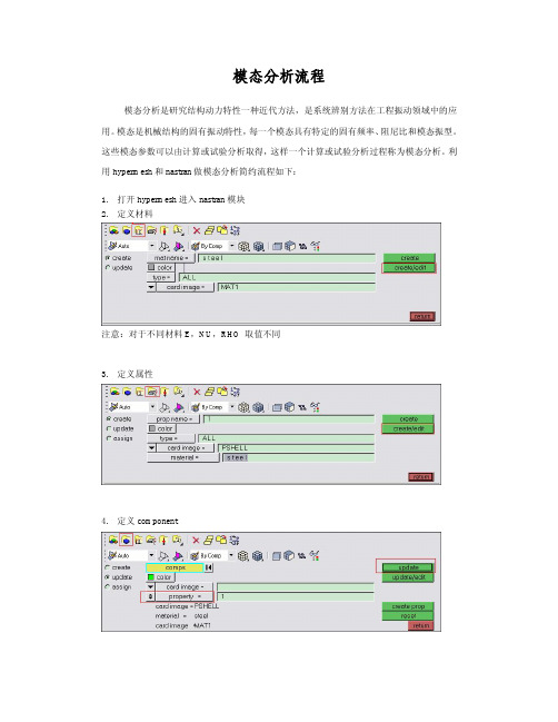
模态分析流程
模态分析是研究结构动力特性一种近代方法，是系统辨别方法在工程振动领域中的应用。

模态是机械结构的固有振动特性，每一个模态具有特定的固有频率、阻尼比和模态振型。

这些模态参数可以由计算或试验分析取得，这样一个计算或试验分析过程称为模态分析。

利用hypermesh和nastran做模态分析简约流程如下：
1.打开hypermesh进入nastran模块
2.定义材料
注意：对于不同材料E，NU，RHO 取值不同
3.定义属性
4.定义component
5.定义力
注意：设置所需模态的阶数，注意前六阶为刚体模态。

6.定义load step
设置SPC和METHOD,类型选择模态
7.定义control card
选择AUTOSPC,BAILOUT为0,DORMM为0,PARAM为-1 8.保存文件，在nastran中进行计算。

基于Hypermesh与ansys的模态分析

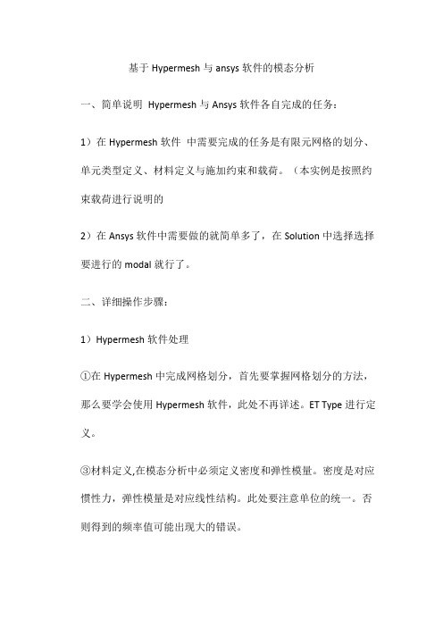
基于Hypermesh与ansys软件的模态分析一、简单说明Hypermesh与Ansys软件各自完成的任务：1）在Hypermesh软件中需要完成的任务是有限元网格的划分、单元类型定义、材料定义与施加约束和载荷。

（本实例是按照约束载荷进行说明的2）在Ansys软件中需要做的就简单多了，在Solution中选择选择要进行的modal就行了。

二、详细操作步骤：1）Hypermesh软件处理①在Hypermesh中完成网格划分，首先要掌握网格划分的方法，那么要学会使用Hypermesh软件，此处不再详述。

ET Type进行定义。

③材料定义,在模态分析中必须定义密度和弹性模量。

密度是对应惯性力，弹性模量是对应线性结构。

此处要注意单位的统一。

否则得到的频率值可能出现大的错误。

④施加约束和载荷（当然在Ansys中做谐响应分析时可以不在Hypermesh中施加载荷）⑤以上步骤完成之后，就要在Ansys进行模态分析。

在进行模态分析之前我们还是要注意出现的问题，这部分是本文说明的重点。

首先，其实当把网格完成之后，还需要删除三维网格以外的单元，比如二维单元、实体模型，这些都会影响有限单元的导入。

我们在划分网格时候为了方便划分网格会进行切割，同样的在我们完成网格之后还要把他们进行组合，可以用Tool中的Organize命令。

我们还会根据不同的零部件产生不同的Component，后面付给不同的单元类型要用到。

第二点，单元类型必须在Hypermesh中定义，不然无法保存成Ansys可以识别的cbd 格式；第三点，当我们完成单元类型的定义和材料属性的定义后，还要做的工作就是在Utility中选择ComponentManager，把我们定义的单元类型和材料付给具有这些性质的Component。

Ansys中打开就不会出现问题了２）Ansys软件处理①在Ansys中需要做的就相对来说简单多了，可以改变Change Jobname，Change Title。

2024新版hypermesh入门基础教程

设置接触条件等方法实现非线性分析。
求解策略
03
采用增量迭代法或牛顿-拉夫逊法进行求解，考虑收敛性和计算
效率。
实例：悬臂梁线性静态分析
问题描述
对一悬臂梁进行线性静态分析，计算其在给定载荷下的位移和应力分布。
分析步骤
建立悬臂梁模型，定义材料属性和边界条件；对模型进行网格划分；施加集中力载荷；设置求解选项并提交求解；查看和评估结果。
HyperMesh实现方法利用OptiStruct求解器进行结构优化，包括拓扑优化、形状优化和尺寸优化等。
3
案例分析
以某车型车架为例，介绍如何在HyperMesh中进行拓扑优化和形状优化，提高车架刚度并降低质量。
疲劳寿命预测技术探讨
01
疲劳寿命预测原理
基于材料疲劳性能、载荷历程等，采用疲劳累积损伤理论进行寿命预测。
HyperMesh实现方法
利用多物理场分析模块，定义各物理场的属性、边界条件等，进行耦合分析。
案例分析
以某电子设备散热问题为例，介绍如何在 HyperMesh中进行结构-热耦合分析，评估设备的散热性能。
实例：汽车车身结构优化
问题描述
针对某车型车身结构，进行刚度、模态及碰撞性能等多目标优化。
01
02
HyperMesh实现方法
利用疲劳分析模块，定义材料疲劳属性、载荷历程等，进行疲劳寿命计算。
03
案例分析
以某车型悬挂系统为例，介绍如何在HyperMesh中进行疲劳寿命预测，评估悬挂系统的耐久性。
多物理场耦合分析简介
多物理场耦合分析原理
考虑多个物理场（如结构、热、流体等）之间的相互作用，进行综合分析。

hypermesh模态动刚度分析流程

hypermesh模态动刚度分析流程下载温馨提示:该文档是我店铺精心编制而成，希望大家下载以后，能够帮助大家解决实际的问题。

文档下载后可定制随意修改，请根据实际需要进行相应的调整和使用，谢谢!并且，本店铺为大家提供各种各样类型的实用资料，如教育随笔、日记赏析、句子摘抄、古诗大全、经典美文、话题作文、工作总结、词语解析、文案摘录、其他资料等等，如想了解不同资料格式和写法，敬请关注!Download tips: This document is carefully compiled by theeditor.I hope that after you download them,they can help yousolve practical problems. The document can be customized andmodified after downloading,please adjust and use it according toactual needs, thank you!In addition, our shop provides you with various types ofpractical materials,such as educational essays, diaryappreciation,sentence excerpts,ancient poems,classic articles,topic composition,work summary,word parsing,copy excerpts,other materials and so on,want to know different data formats andwriting methods,please pay attention!Hypermesh模态动刚度分析流程详解Hypermesh是一款强大的三维几何建模和有限元前处理软件，广泛应用于结构动力学分析中。

hypermesh模态分析

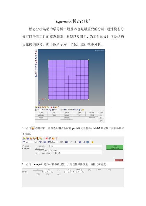
hypermesh模态分析
模态分析是动力学分析中最基本也是最重要的分析，通过模态分析可以得到工件的模态频率，振型以及阻尼，为工件的设计以及结构优化提供参考。

如下图所示为一平板，进行模态分析。

1、点击创建材料，本例选用铝合金材料ge各项同性材料，MM-T单位制，具体参数如下所示。

2、点击create/edit进行材料参数设置，只需设置弹性模量、泊松比和密度。

3、点击进行属性建立，设置如下图所示，2d单元，pshell单元，选取之前建立好的材料AL。

4、create/edit进行参数设置，设置厚度T=1点击return，属性设置完毕。

4、点击把属性赋予单元。

选择assign，comps选择平板，property选择之前建好的属性，点击assign，给网格赋予属性。

5、建立SPC约束，点击，设置如下，点击creat。

6、点击anasys，选择constrain，node选择要约束的点，点击creat，设置如下。

7、点击，card image选择eigrl，设置如下，点击creat/edit。

8、设置模态求解范围v1、v2为求解模态范围，ND为阶数，本例子求解前六阶模态。

9、点击analysis面板loadsteps，进行工况设置。

输入名字type选择mormal modes，spc选
择设置好的SPC,METHOD选择eigrl，点击creat，
10、点击edit，output选择displacement
11、设置完毕可以进行求解啦，本例用optistruct求解第一阶模态振型如下所示。

HyperMesh模态分析步骤

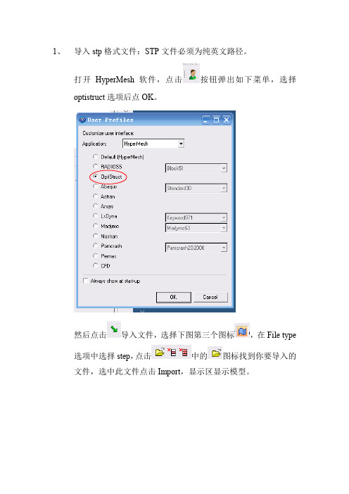
1、导入stp格式文件：STP文件必须为纯英文路径。

打开HyperMesh软件，点击按钮弹出如下菜单，选择optistruct选项后点OK。

然后点击导入文件，选择下图第三个图标，在File type 选项中选择step，点击中的图标找到你要导入的文件，选中此文件点击Import，显示区显示模型。

2、划分自由网格。

软件右下方选中3D选项，然后选择县市区下方网格划分tetramesh选项。

然后选择volume tetra选项，在element size中输入网格的大小根据模型的大小输入数值，此处我输入10，然后选中你要划分的模型变成白颜色，在点击mesh开始划分网格。

等到网格划分结束无错误，点击return返回。

左下提示栏显示为网格划分完成可以下一步操作。

3、创建定义材料。

选择右上处次位置中的model选项在变化的后的下方空白处点击右键，点击下弹菜单中create→Material菜单弹出下图，给定一个英文名字（可以不改为默认），Card image选项中选中MAT1选项，然后点击Create/Edit。

如入材料的弹性模量E、泊松比NU、密度RHO（密度单位为T/mm3一般为负9次方）。

其它都不用选择。

点击return返回。

4、创建单元属性。

还在上次的空白处点击右键，点击下弹菜单中create→property 菜单弹出下图，给定一个英文名字（可以不改为默认），Card image选项中选中PSOLID选项，再在Material选项中选中上一步你定义材料的名字***。

然后点击Create(别点错)。

5、单元属性赋予给材料。

点击软件下面菜单中的第二个图标如下图，选择update选项后，点击黄色的comps选项进入下一菜单，勾选aotu1选项后，点击右下边select，返回上一界面。

点击noproperty更改成property，再在其后面要填写的空格中点击进入选择上一步你命名的单元属性名字后自动返回上一界面。

基于无网格的数值模态匹配法求解消声器声学特性

基于无网格的数值模态匹配法求解消声器声学特性左继强;刘成洋;方智【摘要】应用全局弱式无网格方法求解消声器的横向模态,使用模态匹配技术求解其传递损失.计算了圆形穿孔管阻性消声器的横向模态和传递损失,计算结果与解析方法和有限元方法计算结果吻合较好,且节省计算时间.%The transversal modes of silencers are extracted by using the global weak-form mesh-free method (MFM), and the transmission loss (TL) is calculated by using the mode matching technique. The transversal modes and TL calculation results of a circular perforated dissipative silencer are presented to validate the computational accuracy and the efficiency of the proposed technique.【期刊名称】《噪声与振动控制》【年(卷),期】2018(038)0z1【总页数】5页(P188-192)【关键词】声学;消声器;横向模态;传递损失;全局弱式无网格方法;模态匹配法【作者】左继强;刘成洋;方智【作者单位】华中科技大学船舶与海洋工程学院,武汉 430074;中国舰船研究设计中心,武汉 430064;华中科技大学船舶与海洋工程学院,武汉 430074【正文语种】中文【中图分类】TK421求解消声器声学特性常用的方法有解析方法和数值方法。

解析方法[1]求解简单、快速、精确，但是仅局限于有解析方程的横截面。

对于任意形状的消声器，只能使用数值方法[2]，现在较为成熟的常用的数值方法为有限元方法（FEM）和边界元方法(BEM)。

从hypermesh到nastran——模态和瞬态动力学分析关键步骤设置

hypermesh——nastran——模态分析。

模态分析关键步骤：1. 创建一个load collector, card image选择EIGRL(LANCZOS方法)。

然后editV1 –V2为频率范围，ND为阶数及方程组解的个数。

两者随意选择一个。

2. 创建loadstep，type为normal modes, method选中刚才创建的load collector。

3. 在control cards的sol选择nomal modes，, 如果想生成op2文件，把post也选上值为-1.4. 导出成bdf文件，启动nastran进行分析。

瞬态动力学分析如果激励是力比较好作，如果是强迫位移，老版本的需要用大质量或大刚度法把位移转换成力的载荷。

nastran 2001版以后可以直接加位移，关键步骤如下：1. 定义随时间历程曲线，创建load collectors，card image为Tabled12. 创建瞬态相应的时间步长和时间，load collectors, card image为Tstep3. 创建一个load collectors，card image为DAREA(如果是强迫位移不能用DAREA）4. 创建一个load collectors，card image为Tload1, excited选择DAREA，TID选择TSTEP，注意TYPE的选择。

5. 创建一个subcase，类型选择直接瞬态分析，DLOAD和TSTEP选择刚才创建的两个相对应的load collectors6. 导出成bdf文件，提交nastran进行分析。

如果是强迫位移，还要多两个卡，就是SPCD, LSEQ详细步骤跟以上差不多，只要把各个卡片弄懂了就很容易了。

hyperworks模态分析实例教程

Normal Modes Analysis of a Splash Shield - RD-1020In this tutorial, an existing finite element model of an automotive splash shield will be used to demonstrate how to set up and perform a normal modes analysis. HyperMesh post-processing tools are used to determine mode shapes of the model.The following exercises are included:•Retrieving the RADIOSS input file•Setting up the model in HyperMesh•Applying Loads and Boundary Conditions to the Model•Submitting the job•Viewing the resultsStep 1: Launch HyperMesh and set the RADIOSS (Bulk Data) User Profileunch HyperMesh.A User Profiles… Graphic User Interface (GUI) will appear. If it does not appear, go to Preferences►User Profiles … from the menu on the top.2.Select RADIOSS in the User Profile dialog.3.From the extended list, select Bulk Data.4.Click OK.This loads the User Profile. It includes the appropriate template, macro menu, and import reader, paring down the functionality of HyperMesh to what is relevant for generating models in Bulk Data Format for RADIOSS and OptiStruct.Step 2: Import a Finite Element Model File in HyperMesh1.From the File pull-down menu on the toolbar, select Import….An Import… tab is added to your tab menu.2.Click to import an FE model.3.For the File type:, select RADIOSS (Bulk Data).4.Select the Files icon button.A Select RADIOSS (Bulk Data) file browser will pop up.5.Browse for sshield.fem file located in the HyperWorks installation directory under<install_directory>/tutorials/hwsolvers/radioss/ and select the file.6.Click Open►Import.7.Click Close to close the Import tab menu.Step 3: Review Rigid ElementsNotice there are two rigid "spiders" in the model. They are placed at locations where the shield is bolted down. This is a simplified representation of the interaction between the bolts and the shield. It is assumed that the bolts are significantly more rigid in comparison to the shield.The dependent nodes of the rigid elements have all six degrees of freedom constrained. Therefore, each "spider" connects nodes of the shell mesh together in such a way that they do not move with respect to one another.The following steps show how to review the properties of the rigid elements.1.From the 1D page, select the rigids.2.Click review.3.Select one of the rigid elements in the graphics region.In the graphics window, HyperMesh displays the IDs of the rigid element and the two end nodes and indicates the independent node with an 'I' and the dependent node with a 'D'. HyperMesh also indicates the constrained degrees of freedom for the selected element, through the dof checkboxes in the rigids panel. All rigid elements in this model should have all dofs constrained.4.Click return to go to the main menu.Step 4: Setting up the Material and Geometric PropertiesThe imported model has three component collectors with no materials. A material collector needs to be created and assigned to the shell component collectors. The rigid elements do not need to be assigned a material. Shell thickness values also need to be corrected.1.Select the Material Collectors toolbar button .2.Select the create subpanel using the radio buttons on the left-hand side of the panel.3.Click mat name = and enter steel.4.Select the desired color for the material steel by clicking on .5.Click card image = and select MAT1 from the pop-up menu.6.Click create/edit.The MAT1 card image pops up.7.For E, enter the value 2.0E5.8.For NU, enter the value 0.3.9.For RHO, enter the value 7.85E-9.If a quantity in brackets does not have a value below it, it is off. To change this, click the quantity in brackets and an entry field will appear below it. Click in the entry field, and a value can be entered.10.Click return.A new material, steel, has now been created. The material uses RADIOSS linear isotropic materialmodel, MAT1. This material has a Young's Modulus of 2E+05, a Poisson's Ratio of 0.3 and a material density of 7.85E-09. A material density is required for the normal modes solution sequence.At any time the card image for this collector can be modified using Card Editor.11.Click return to exit the Material Create panel.12.Select the Card Editor toolbar button .13.Click the down arrow on the right of the entity shown in the yellow box, select props from the extendedentity list.14.Click the yellow props button and then check the box next to design and nondesign.15.Click select.16.Make sure card image=is set to PSHELL.17.Click edit.The PSHELL card image for the design component collector pops up.18.Replace 0.300 in the T field with 0.25.19.Click return to save the changes to the card image.20.Click return to go to the main menu.Applying Loads and Boundary Conditions to the Model (Steps 5 - 7)The model is to be constrained using SPCs at the bolt locations, as shown in the following figure. The constraints will be organized into the load collector 'constraints'.To perform a normal modes analysis, a real eigenvalue extraction (EIGRL) card needs to be referenced in the subcase. The real eigenvalue extraction card is defined in HyperMesh as a load collector with an EIGRL card image. This load collector should not contain any other loads.Step 5: Create EIGRL card (to request the number of modes)If a quantity in brackets does not have a value below it, it is off. To change this, click on the quantity in brackets and an entry field will appear below it. Click on the entry field, and a value can be entered.Step 6: Create Constraints at Bolt LocationsSelecting nodes for constraining the bolt locations 1.Click the Load Collectors toolbar button .2.Select the create subpanel, using the radio buttons on the left-hand side of the panel.3.Click loadcol name = and enter EIGRL .4.Click card image= and select EIGRL from the pop-up menu.5.Click create/edit .6.For V2, enter the value 200.000.7.For ND , enter the value 6.8.Click return to save changes to the card image.1.Click loadcol name = and enter constraints .2.Click the switch next to card image and select no card image .3.Click create > return .4.From Analysis page, click the constraints panel and make sure that the createsubpanel is active.5.Select the two nodes, shown in the figure above, at the center of the rigid spiders, by clicking on them in the graphics window.6.Constrain all dofs with a value of 0.0.7.Click Load Type= and select SPC .8.Click createTwo constraints are created. Constraint symbols (triangles) appear in the graphics window at theselected nodes. The number 123456 is written beside the constraint symbol, if the label constraints is checked ‘ON’, indicating that all dofs are constrained.9.Click return to go the main menu.Step 7: Create a Load Step to perform Normal Modes Analysis1.From the Analysis page, enter the loadsteps panel.2.Click name = and enter bolted.3.Click the type: switch and select normal modes from the pop-up menu.4.Check the box preceding SPC.An entry field appears to the right of SPC.5.Click on the entry field and select constraints from the list of load collectors.6.Check the box preceding METHOD(STRUCT).An entry field appears to the right of METHOD.7.Click on the entry field and select EIGRL from the list of load collectors.8.Click create.A RADIOSS subcase has been created which references the constraints in the load collector constraintsand the real eigenvalue extraction data in the load collector EIGRL.9.Click return to go to the main menu.Submitting the JobStep 8: Running Normal Modes Analysis1.From the Analysis page, enter the RADIOSS panel.2.Click save as… following the input file:field.A Save file… browser window pops up.3.Select the directory where you would like to write the file and, in File name:, entersshield_complete.fem.4.Click Save.Note that the name and location of the sshield_complete.fem file shows in the input file: field.5.Set the export options:toggle to all.6.Click the run options: switch and select analysis.7.Set the memory options: toggle to memory default.8.Click Radioss.This launches the RADIOSS job.If the job was successful, new results files can be seen in the directory where the RADIOSS model file was written. The sshield_complete.out file is a good place to look for error messages that will help to debug the input deck if any errors are present.The default files written to your directory are:sshield_complete.html HTML report of the analysis, giving a summary of the problemformulation and the analysis results.sshield_complete.out RADIOSS output file containing specific information on the file setup, the set up of your optimization problem, estimates for the amountof RAM and disk space required for the run, information for eachoptimization iteration, and compute time information. Review this fileReview the Results using HyperViewEigenvector results are output by default, from RADIOSS for a normal modes analysis. This section describes how to view the results in HyperView.Step 9: Load the Model and Result Files into the Animation WindowIn this section, you will load a HyperView .h3d file into the HyperView animation window.HyperView is launched and the sshield_complete.h3d file is loaded.Step 10: View Eigen VectorsIt is helpful to view the deformed shape of a model to determine if the boundary conditions have been defined correctly and also to check if the model is deforming as expected. In this section, use the Deformed panel to review the deformed shape for last Mode .This means that the maximum displacement will be 10 modal units and all other displacements will be proportional.Using a scale factor higher than 1.0 amplifies the deformations while a scale factor smaller than 1.0 would reduce them. In this case, we are accentuating displacements in all directions.A deformed plot of the model overlaid on the original undeformed mesh is displayed in the graphics window. for warnings and errors.sshield_complete.h3dHyper 3D binary results file. sshield_complete.stat Summary of analysis process, providing CPU information for eachstep during analysis process. 1.Click the HyperView button in the RADIOSS panel. 2.Click Close to exit the Message Log menu that appears.1.Click on the switch next to the traffic light signaland select Modal .2.Select the Deformed toolbar button.3.Leave Result type:set to Eigen Mode (v).4.Set Scale: to Model units .5.Set Type: to Uniform and enter in a scale factor of 10 for Value:.6.Click Apply .7.Under Undeformed shape:, set Show: to Wireframe .8.From the Graphics pull-down menu, select Select Load Case to activate the Load Case andSimulation Selection dialog, as shown below.Step 11: A few points to be notedIn this analysis, it was assumed that the bolts were significantly stiffer than the shield. If the bolts needed to be made of aluminum and the shield was still made of steel, would the model need to be modified, and the analysis run again?It is necessary to push the natural frequencies of the splash shield above 50 Hz. With the current model, there should be one mode that violates this constraint: Mode 1. Design specifications allow the innerdisjointed circular rib to be modified such that no significant mass is added to the part. Is there a configuration for this rib within the above stated constraints that will push the first mode above 50 Hz? See tutorial OS-2020 to optimize rib locations for this part.Go ToRADIOSS, MotionSolve, and OptiStruct Tutorials9.Select Mode 6 - F=1.496557E+02 from the list and click OK to view Mode 6.10.To animate the mode shape, click the animation mode: modal.11.To control the animation speed, use the Animation Controls accessed with the director’s chair toolbar button .12.You could also review the rest of the mode shapes.。

hyperworks模态分析实例教程

Normal Modes Analysis of a Splash Shield - RD-1020In this tutorial, an existing finite element model of an automotive splash shield will be used to demonstrate how to set up and perform a normal modes analysis. HyperMesh post-processing tools are used to determine mode shapes of the model.The following exercises are included:•Retrieving the RADIOSS input file•Setting up the model in HyperMesh•Applying Loads and Boundary Conditions to the Model•Submitting the job•Viewing the resultsStep 1: Launch HyperMesh and set the RADIOSS (Bulk Data) User Profileunch HyperMesh.A User Profiles… Graphic User Interface (GUI) will appear. If it does not appear, go to Preferences►User Profiles … from the menu on the top.2.Select RADIOSS in the User Profile dialog.3.From the extended list, select Bulk Data.4.Click OK.This loads the User Profile. It includes the appropriate template, macro menu, and import reader, paring down the functionality of HyperMesh to what is relevant for generating models in Bulk Data Format for RADIOSS and OptiStruct.Step 2: Import a Finite Element Model File in HyperMesh1.From the File pull-down menu on the toolbar, select Import….An Import… tab is added to your tab menu.2.Click to import an FE model.3.For the File type:, select RADIOSS (Bulk Data).4.Select the Files icon button.A Select RADIOSS (Bulk Data) file browser will pop up.5.Browse for sshield.fem file located in the HyperWorks installation directory under<install_directory>/tutorials/hwsolvers/radioss/ and select the file.6.Click Open►Import.7.Click Close to close the Import tab menu.Step 3: Review Rigid ElementsNotice there are two rigid "spiders" in the model. They are placed at locations where the shield is bolted down. This is a simplified representation of the interaction between the bolts and the shield. It is assumed that the bolts are significantly more rigid in comparison to the shield.The dependent nodes of the rigid elements have all six degrees of freedom constrained. Therefore, each "spider" connects nodes of the shell mesh together in such a way that they do not move with respect to one another.The following steps show how to review the properties of the rigid elements.1.From the 1D page, select the rigids.2.Click review.3.Select one of the rigid elements in the graphics region.In the graphics window, HyperMesh displays the IDs of the rigid element and the two end nodes and indicates the independent node with an 'I' and the dependent node with a 'D'. HyperMesh also indicates the constrained degrees of freedom for the selected element, through the dof checkboxes in the rigids panel. All rigid elements in this model should have all dofs constrained.4.Click return to go to the main menu.Step 4: Setting up the Material and Geometric PropertiesThe imported model has three component collectors with no materials. A material collector needs to be created and assigned to the shell component collectors. The rigid elements do not need to be assigned a material. Shell thickness values also need to be corrected.1.Select the Material Collectors toolbar button .2.Select the create subpanel using the radio buttons on the left-hand side of the panel.3.Click mat name = and enter steel.4.Select the desired color for the material steel by clicking on .5.Click card image = and select MAT1 from the pop-up menu.6.Click create/edit.The MAT1 card image pops up.7.For E, enter the value 2.0E5.8.For NU, enter the value 0.3.9.For RHO, enter the value 7.85E-9.If a quantity in brackets does not have a value below it, it is off. To change this, click the quantity in brackets and an entry field will appear below it. Click in the entry field, and a value can be entered.10.Click return.A new material, steel, has now been created. The material uses RADIOSS linear isotropic materialmodel, MAT1. This material has a Young's Modulus of 2E+05, a Poisson's Ratio of 0.3 and a material density of 7.85E-09. A material density is required for the normal modes solution sequence.At any time the card image for this collector can be modified using Card Editor.11.Click return to exit the Material Create panel.12.Select the Card Editor toolbar button .13.Click the down arrow on the right of the entity shown in the yellow box, select props from the extendedentity list.14.Click the yellow props button and then check the box next to design and nondesign.15.Click select.16.Make sure card image=is set to PSHELL.17.Click edit.The PSHELL card image for the design component collector pops up.18.Replace 0.300 in the T field with 0.25.19.Click return to save the changes to the card image.20.Click return to go to the main menu.Applying Loads and Boundary Conditions to the Model (Steps 5 - 7)The model is to be constrained using SPCs at the bolt locations, as shown in the following figure. The constraints will be organized into the load collector 'constraints'.To perform a normal modes analysis, a real eigenvalue extraction (EIGRL) card needs to be referenced in the subcase. The real eigenvalue extraction card is defined in HyperMesh as a load collector with an EIGRL card image. This load collector should not contain any other loads.Step 5: Create EIGRL card (to request the number of modes)If a quantity in brackets does not have a value below it, it is off. To change this, click on the quantity in brackets and an entry field will appear below it. Click on the entry field, and a value can be entered.Step 6: Create Constraints at Bolt LocationsSelecting nodes for constraining the bolt locations 1.Click the Load Collectors toolbar button .2.Select the create subpanel, using the radio buttons on the left-hand side of the panel.3.Click loadcol name = and enter EIGRL .4.Click card image= and select EIGRL from the pop-up menu.5.Click create/edit .6.For V2, enter the value 200.000.7.For ND , enter the value 6.8.Click return to save changes to the card image.1.Click loadcol name = and enter constraints .2.Click the switch next to card image and select no card image .3.Click create > return .4.From Analysis page, click the constraints panel and make sure that the createsubpanel is active.5.Select the two nodes, shown in the figure above, at the center of the rigid spiders, by clicking on them in the graphics window.6.Constrain all dofs with a value of 0.0.7.Click Load Type= and select SPC .8.Click createTwo constraints are created. Constraint symbols (triangles) appear in the graphics window at theselected nodes. The number 123456 is written beside the constraint symbol, if the label constraints is checked ‘ON’, indicating that all dofs are constrained.9.Click return to go the main menu.Step 7: Create a Load Step to perform Normal Modes Analysis1.From the Analysis page, enter the loadsteps panel.2.Click name = and enter bolted.3.Click the type: switch and select normal modes from the pop-up menu.4.Check the box preceding SPC.An entry field appears to the right of SPC.5.Click on the entry field and select constraints from the list of load collectors.6.Check the box preceding METHOD(STRUCT).An entry field appears to the right of METHOD.7.Click on the entry field and select EIGRL from the list of load collectors.8.Click create.A RADIOSS subcase has been created which references the constraints in the load collector constraintsand the real eigenvalue extraction data in the load collector EIGRL.9.Click return to go to the main menu.Submitting the JobStep 8: Running Normal Modes Analysis1.From the Analysis page, enter the RADIOSS panel.2.Click save as… following the input file:field.A Save file… browser window pops up.3.Select the directory where you would like to write the file and, in File name:, entersshield_complete.fem.4.Click Save.Note that the name and location of the sshield_complete.fem file shows in the input file: field.5.Set the export options:toggle to all.6.Click the run options: switch and select analysis.7.Set the memory options: toggle to memory default.8.Click Radioss.This launches the RADIOSS job.If the job was successful, new results files can be seen in the directory where the RADIOSS model file was written. The sshield_complete.out file is a good place to look for error messages that will help to debug the input deck if any errors are present.The default files written to your directory are:sshield_complete.html HTML report of the analysis, giving a summary of the problemformulation and the analysis results.sshield_complete.out RADIOSS output file containing specific information on the file setup, the set up of your optimization problem, estimates for the amountof RAM and disk space required for the run, information for eachoptimization iteration, and compute time information. Review this fileReview the Results using HyperViewEigenvector results are output by default, from RADIOSS for a normal modes analysis. This section describes how to view the results in HyperView.Step 9: Load the Model and Result Files into the Animation WindowIn this section, you will load a HyperView .h3d file into the HyperView animation window.HyperView is launched and the sshield_complete.h3d file is loaded.Step 10: View Eigen VectorsIt is helpful to view the deformed shape of a model to determine if the boundary conditions have been defined correctly and also to check if the model is deforming as expected. In this section, use the Deformed panel to review the deformed shape for last Mode .This means that the maximum displacement will be 10 modal units and all other displacements will be proportional.Using a scale factor higher than 1.0 amplifies the deformations while a scale factor smaller than 1.0 would reduce them. In this case, we are accentuating displacements in all directions.A deformed plot of the model overlaid on the original undeformed mesh is displayed in the graphics window. for warnings and errors.sshield_complete.h3dHyper 3D binary results file. sshield_complete.stat Summary of analysis process, providing CPU information for eachstep during analysis process. 1.Click the HyperView button in the RADIOSS panel. 2.Click Close to exit the Message Log menu that appears.1.Click on the switch next to the traffic light signaland select Modal .2.Select the Deformed toolbar button.3.Leave Result type:set to Eigen Mode (v).4.Set Scale: to Model units .5.Set Type: to Uniform and enter in a scale factor of 10 for Value:.6.Click Apply .7.Under Undeformed shape:, set Show: to Wireframe .8.From the Graphics pull-down menu, select Select Load Case to activate the Load Case andSimulation Selection dialog, as shown below.Step 11: A few points to be notedIn this analysis, it was assumed that the bolts were significantly stiffer than the shield. If the bolts needed to be made of aluminum and the shield was still made of steel, would the model need to be modified, and the analysis run again?It is necessary to push the natural frequencies of the splash shield above 50 Hz. With the current model, there should be one mode that violates this constraint: Mode 1. Design specifications allow the innerdisjointed circular rib to be modified such that no significant mass is added to the part. Is there a configuration for this rib within the above stated constraints that will push the first mode above 50 Hz? See tutorial OS-2020 to optimize rib locations for this part.Go ToRADIOSS, MotionSolve, and OptiStruct Tutorials9.Select Mode 6 - F=1.496557E+02 from the list and click OK to view Mode 6.10.To animate the mode shape, click the animation mode: modal.11.To control the animation speed, use the Animation Controls accessed with the director’s chair toolbar button .12.You could also review the rest of the mode shapes.。

Hypermesh与Nastran模态分析详细教程

Hypermesh & Nastran 模态分析教程摘要：本文将采用一个简单外伸梁的例子来讲述Hypemesh 与Nastran 联合仿真进行模态分析的全过程。

教程内容:1.打开”Hypermesh 14.0”进入操作界面，在弹出的对话框上勾选‘nastran’模块，点‘ok’，如图1.1 所示。

图1.1-hypermesh 主界面2.梁结构网格模型的创建在主界面左侧模型树空白处右击选择‘Creat’ –‘Component’,重命名为‘BEAM’，然后创建尺寸为100*10*5mm3的梁结构网格模型。

（一开始选择了Nastran后，单位制默认为N, ton, MPa, mm.）。

本例子网格尺寸大小为2.5*2.5*2.5mm3，如图2.1 所示：图2.1-梁结构网格模型3.定义网格模型材料属性●在主界面左侧模型树空白处右击选择‘Creat’–‘Material’，如图3.1所示：图3.1-材料创建●在模型树内Material下将出现新建的材料‘Material 1’，将其重命名为’BEAM’。

点击‘BEAM’,将会出现材料参数设置对话框。

本例子采用铁作为梁结构材料，对于模态分析，我们只需要设定材料弹性模量，泊松比，密度即可。

故在参数设置对话框内填入一下数据：完整的材料参数设置如图3.2所示：图3.2-Material材料参数设置同理，按同样方式在主界面左侧模型树空白处右击选择‘Creat’ –‘Pro perty’，模型树上Property下将出现新建的‘Property1’，同样将其重命名为‘BEAM’，点击Property下的‘BEAM’出现如图所示属性参数设置对话框。

由于本例子使用的单元为三维体单元，因此点击对话框的‘card image’选择‘PSOLID’，点击对话框内的Material选项，选择上一步我们设置好的材料‘BEAM’，完整的设置如图3.3所示：图3.3-Property属性设置最后，点击之前创建的在Component 下的‘BEAM’模型，将出现以下对话框（图3.4），把Property 和Material 都选上对应的‘BEAM’，完成网格模型材料属性的定义。

HyperMesh软件在消声器声学特性分析中的应用

HyperMesh软件在消声器声学特性分析中的应用张冬莲赵立峰杨亮重庆长安汽车工程研究总院重庆401120摘要:设计高消声性能、低压力损失的排气系统是噪声控制中的重要课题。

HyperMesh软件能对穿孔管、穿孔板、吸声材料等准确建模进而进行有限元仿真分析，是排气系统性能预测和改进设计的有效方法。

本文针对某发动机排气系统的前、后消声器进行了消声特性的三维传递损失仿真分析，并与试验数据进行了对比，得出传递损失的三维仿真结果与试验结果吻合较好。

因此在消声器的前期设计中可以通过分析消声器本身的消声特性来预测此消声器的消声作用并根据结果对消声器结构进行改进设计，从而指导实际工程问题。

关键词：排气消声器，有限元，传递损失，HyperMesh1 引言排气系统一直以来都是发动机最大的噪声源。

而消声元件本身的消声特性是控制噪声的关键所在，因此如何设计高消声性能、低压力损失的排气系统是噪声控制的根本。

本文以某轿车的排气系统为例，利用HyperMesh软件建立前后消声器的三维有限元模型，利用Sysnoise软件进行消声器的三维传递损失分析。

并在HyperMesh软件中通过将穿孔管、穿孔板上的小圆孔等效成四边形方孔和六边形方孔两种情况来研究穿孔管、穿孔板上孔的形状对传递损失的影响，以便在后期仿真分析中缩短建模时间、减小有限元单元数量及提高仿真精度。

2 排气系统声学特性三维有限元分析2.1三维有限元模型本文研究的排气系统主要包括两级消声器和连接消声器的进出口长管。

由于缺少三元催化器的相关结构参数，而且三元催化器主要用于改善发动机的排放，而不是消声性能和空气动力性能，所以排气系统建模时不考虑三元催化器。

消声器内部的穿孔管、穿孔板、吸声材料均采用实体建模。

排气系统的几何模型及前后消声器的有限元模型见图1、图2、图3。

2.2三维传递损失计算计算模型为图2、图3中的消声器有限元模型，其中紫色部分表示吸声材料所加位置。

入口施加了单位速度激励，出口施加了吸声系数为1的全部吸收边界，本文暂不考虑温度、流速对消声性能的影响，表1列出了空气及吸声材料的属性。

基于HyperMesh_的挖掘机消音器结构优化设计

基于HyperMesh的挖掘机消音器结构优化设计俞松松，陈江飞，赵卫东，陈松生（广西柳工机械股份有限公司，广西柳州 545007）［摘要］针对某小型液压挖掘机消音器排气尾管断裂问题，运用HyperMesh对其进行模态分析，得到消音器前6阶模态振型，初步判断引起排气尾管断裂的模态振型。

对排气尾管进行振动测试，通过频谱分析，其振动频率与消音器1阶频率接近，证明了有限元建模的准确性，并确定了排气尾管断裂的根本原因为消音器1阶频率与激励频率共振。

对消音器进行谐响应分析，得到消音器刚度最弱位置与实际断裂位置一致，对消音器结构进行优化，避开发动机激励频率，解决了排气尾管与发动机激励共振问题。

目前挖掘机已工作2000h以上，未发现消音器排气尾管开裂，证明了失效原因分析及改进方法的正确性。

［关键词］消音器；共振；模态分析；谐响应分析［中图分类号］TU621 ［文献标识码］A ［文章编号］1001-554X（2023）06-0147-05Optimization design of excavator silencer structure based on HyperMesh YU Song-song，CHEN Jiang-fei，ZHAO Wei-dong，CHEN Song-sheng由于小型挖掘机多数在城市内进行施工，其噪声大小成为客户及主机厂关注的重要指标。

作为降低挖掘机排气噪声的关键零部件，消音器除了需要具备高效的降噪功能，其高可靠性和耐久性也是设计师重点考虑的因素。

由于小型挖掘机空间较狭窄，大部分消音器直接与发动机本体刚性连接，在进行消音器的设计时，需考虑消音器刚度、质量和阻尼等参数，避免与发动机激励、挖掘作业激励、排气激励等产生共振。

针对某小型液压挖掘机排气系统中的消声器排气尾管在可靠性试验验证工作约800h后出现断裂的问题，运用拉格朗日方程对排气系统进行动力学理论分析［1］；利用HyperMesh进行有限元分析，通过模态分析得到消音器的模态频率和振型，通过谐响应分析找到消音器最薄弱的位置；结合实测振动数据分析、有限元方法得到系统模态振型；通过谐响应分析得出排气系统刚度最弱，结合试验数据分析确定某型挖掘机消音器排气尾管断裂为排气尾管与发动机激励共振所致；通过对消音器结构参数进行优化，并通过模态分析、谐响应分析及试验测试，解决了消音器排气尾管共振问题，证明了该分析方法的正确性。

汽车排气系统总成模态分析

汽车排气系统总成模态分析作者：王帅杜长远杨蓓来源：《科技视界》2020年第19期摘要汽车排气系统的振动对汽车舒适性和排气系统寿命有重要的影响，文章利用SolidWorks 软件建立某轿车排气系统的装配体模型，利用HyperMesh和ANSYS联合仿真有限元分析方法，对汽车排气管后消声器总成模型进行模态分析。

通过模态分析结果，分析汽车排气系统振动频率及危险位置，分析结果对相关排气系统后消声器总成设备进行优化设计有指导意义。

关键词汽车排气系统;模态分析;有限元方法中图分类号： U464.134.4 ; ; ; 文献标识码： ADOI：10.19694/ki.issn2095-2457.2020.19.018AbstractThe vibration of the car’s exhaust system has an important influence on the comfort of the car and the life of the exhaust system.In this paper，the SolidWorks software is used to build the assembly model of a car exhaust system. The modal analysis of the rear exhaust muffler assembly model of the automobile exhaust pipe is carried out by Hyper Mesh and ANSYS joint simulation finite element analysis.Through the modal analysis results， the frequency and dangerous position of the vehicle exhaust system vibration are analyzed.The analysis results have important guiding significance for the design of the exhaust muffler assembly exhaust system.Key WordsVehicle exhaust system;Modal analysis;Finite element method0 引言隨着汽车行业的高速发展，汽车轻量化是主要发展方向之一[1]，除了汽车的安全性，汽车的舒适性也越来越受到重视。