比较线性模型和Probit模型、Logit模型
logit 和probit模型的系数解释 -回复

logit 和probit模型的系数解释-回复主题:logit 和probit 模型的系数解释引言logit 模型和probit 模型是广泛应用于概率统计和经济学中的两个模型,用于解释事件发生的概率与相关因素之间的关系。
本文将详细介绍这两个模型的系数解释,并分析它们在实际应用中的区别和适用场景。
一、logit 模型系数解释logit 模型基于二项逻辑回归的概率模型,适用于事件结果是二元变量(如成功/失败,发生/不发生)的情况。
该模型通过计算事件发生的对数几率来建模,并利用最大似然估计来确定系数的值。
1. 系数的正负logit 模型中的系数是事件发生概率对于自变量的变化的影响大小。
系数的正负代表了自变量与事件发生概率之间的正相关或负相关关系。
正系数意味着自变量的增加会增加事件发生概率,而负系数意味着自变量的增加会减少事件发生概率。
2. 系数的大小logit 模型中,系数的大小代表了自变量单位变化对于事件发生概率的影响程度。
系数越大,自变量的一个单位变化对于事件发生概率的影响就越大。
一般来说,当系数的绝对值大于1时,其影响被认为是显著的。
3. 系数的统计显著性logit 模型使用最大似然估计来确定系数的值,同时也提供了对系数是否显著的统计检验。
当系数的p 值小于显著性水平(通常为0.05或0.01)时,我们可以认为该系数是显著的,即具有统计上的置信度。
二、probit 模型系数解释probit 模型是基于正态分布的概率模型,与logit 模型相似,用于解决二元变量的概率建模问题。
不同的是,probit 模型通过计算事件发生的累积分布函数值来建模,并同样利用最大似然估计来确定系数的值。
1. 系数的正负probit 模型中的系数的解释与logit 模型相同,系数的正负代表了自变量与事件发生概率之间的正相关或负相关关系。
正系数意味着自变量的增加会增加事件发生概率,而负系数意味着自变量的增加会减少事件发生概率。
probit模型与logit模型
probit模型与logit模型2013-03-30 16:10:17probit模型是一种广义的线性模型。
服从正态分布。
最简单的probit模型就是指被解释变量Y是一个0,1变量,事件发生地概率是依赖于解释变量,即P(Y=1)=f(X),也就是说,Y=1的概率是一个关于X的函数,其中f(.)服从标准正态分布。
若f(.)是累积分布函数,则其为Logistic模型Logit模型(Logit model,也译作“评定模型”,“分类评定模型”,又作Logistic regression,“逻辑回归”)是离散选择法模型之一,属于多重变量分析范畴,是社会学、生物统计学、临床、数量心理学、市场营销等统计实证分析的常用方法。
逻辑分布(Logistic distribution)公式P(Y=1│X=x)=exp(x’β)/1+exp(x’β)其中参数β常用极大似然估计。
Logit模型是最早的离散选择模型,也是目前应用最广的模型。
Logit模型是Luce(1959)根据IIA特性首次导出的;Marschark(1960)证明了Logit模型与最大效用理论的一致性;Marley (1965)研究了模型的形式和效用非确定项的分布之间的关系,证明了极值分布可以推导出Logit 形式的模型;McFadden(1974)反过来证明了具有Logit形式的模型效用非确定项一定服从极值分布。
此后Logit模型在心理学、社会学、经济学及交通领域得到了广泛的应用,并衍生发展出了其他离散选择模型,形成了完整的离散选择模型体系,如Probit模型、NL模型(Nest Logit model)、Mixed Logit模型等。
模型假设个人n对选择枝j的效用由效用确定项和随机项两部分构成:Logit模型的应用广泛性的原因主要是因为其概率表达式的显性特点,模型的求解速度快,应用方便。
当模型选择集没有发生变化,而仅仅是当各变量的水平发生变化时(如出行时间发生变化),可以方便的求解各选择枝在新环境下的各选择枝的被选概率。
比较线性模型和Probit模型、Logit模型

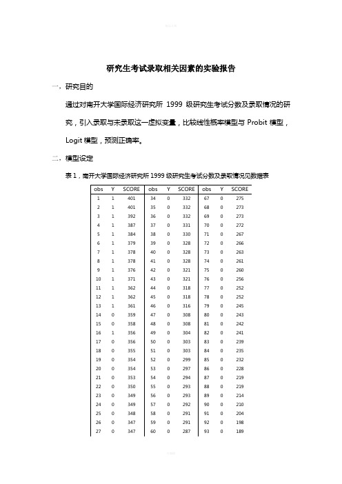
研究生考试录取相关因素的实验报告一,研究目的通过对南开大学国际经济研究所1999级研究生考试分数及录取情况的研究,引入录取与未录取这一虚拟变量,比较线性概率模型与Probit模型,Logit模型,预测正确率。
二,模型设定表1,南开大学国际经济研究所1999级研究生考试分数及录取情况见数据表定义变量。
上图为样本观测值。
1.线性概率模型根据上面资料建立模型用Eviews 得到回归结果如图: Dependent Variable: Y Method: Least Squares Date: 12/10/10 Time: 20:38 Sample: 1 97Included observations: 97 Variable Coefficient Std. Errort-StatisticProb.??C SCORER-squared????Mean dependent var Adjusted R-squared ????. dependent var . of regression ????Akaike info criterion Sum squared resid ????Schwarz criterion Log likelihood ????F-statistic Durbin-Watson stat ????Prob(F-statistic)参数估计结果为: iY ˆ+ i SCORE Se=( t=p=预测正确率:Forecast: YF Actual: YForecast sample: 1 97 Included observations: 97Root Mean Squared Error Mean Absolute Error????? Mean Absolute Percentage Error Theil Inequality Coefficient? ?????Bias Proportion???????? ?????Variance Proportion? ?????Covariance Proportion?模型Dependent Variable: Y Method: ML - Binary Logit (Quadratic hill climbing)Date: 12/10/10 Time: 21:38Sample: 1 97Included observations: 97Convergence achieved after 11 iterationsCovariance matrix computed using second derivatives Variable Coefficient Std. Errorz-StatisticProb.??C SCOREMean dependent var ????. dependent var . of regression ????Akaike info criterion Sum squared resid ????Schwarz criterion Log likelihood ????Hannan-Quinn criter. Restr. log likelihood ????Avg. log likelihood LR statistic (1 df) ????McFadden R-squaredProbability(LR stat)Obs with Dep=0 83 ?????Total obs 97Obs with Dep=1 14得Logit 模型估计结果如下p i = F (y i ) =)6794.07362.243(11i x e +--+ 拐点坐标 ,其中Y=+预测正确率Forecast: YF Actual: YForecast sample: 1 97 Included observations: 97Root Mean Squared Error Mean Absolute Error????? Mean Absolute Percentage Error Theil Inequality Coefficient? ?????Bias Proportion???????? ?????Variance Proportion? ?????Covariance Proportion?模型Dependent Variable: Y Method: ML - Binary Probit (Quadratic hill climbing)Date: 12/10/10 Time: 21:40Sample: 1 97Included observations: 97Convergence achieved after 11 iterationsCovariance matrix computed using second derivativesVariable Coefficient Std. Error z-Statistic Prob.??CSCOREMean dependent var ????. dependent var. of regression ????Akaike info criterionSum squared resid ????Schwarz criterionLog likelihood ????Hannan-Quinn criter.Restr. log likelihood ????Avg. log likelihoodLR statistic (1 df) ????McFadden R-squaredProbability(LR stat)Obs with Dep=0 83 ?????Total obs 97Obs with Dep=1 14Probit模型最终估计结果是p i = F(y i) = F+ x i) 拐点坐标,预测正确率Forecast: YFActual: YForecast sample: 1 97Included observations: 97Root Mean Squared ErrorMean Absolute Error?????Mean Absolute Percentage ErrorTheil Inequality Coefficient??????Bias Proportion?????????????Variance Proportion??????Covariance Proportion?预测正确率结论:线性概率模型RMSE= MAE= MAPE=Logit模型 RMSE= MAE= MAPE=Probit模型 RMSE= MAE= MAPE=由上面结果可知线性概率模型的RMSE、MAE、MAPE 均远远大于Logit模型和Probit模型,说明其误差率比Logit模型和Probit模型大很多,所以正确率远远小于Logit模型和Probit模型。
logit 和probit模型的系数解释 -回复
logit 和probit模型的系数解释-回复Logit和Probit模型是常用的二元选择模型,用于分析二元变量的选择行为。
它们通常用于解释个体在做出选择时的决策,可以帮助我们理解各种影响因素对选择行为的影响。
在这篇文章中,我将逐步回答有关Logit和Probit模型的系数解释的问题,介绍这两个模型的基本原理、模型形式、系数解释和使用注意事项,以及如何解读模型中的系数。
首先,让我们从基本原理开始,了解Logit和Probit模型的背后逻辑。
Logit 和Probit模型都属于广义线性模型(Generalized Linear Models),它们基于一个相似的假设:选择行为是一个概率事件,可以由一组解释变量进行解释。
这些解释变量可以是个体特征(如年龄、性别、教育水平等),也可以是一些特定的因素(如收入水平、市场利率等)。
模型的目的是通过对这些解释变量的分析,预测和解释个体做出选择的概率。
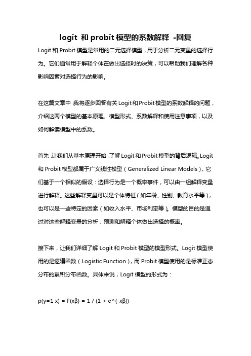
接下来,让我们详细了解Logit和Probit模型的模型形式。
Logit模型使用的是逻辑函数(Logistic Function),而Probit模型使用的是标准正态分布的累积分布函数。
具体来说,Logit模型的形式为:p(y=1 x) = F(xβ) = 1 / (1 + e^(-xβ))其中,p(y=1 x)表示个体在给定解释变量x的情况下选择y=1的概率,F(x β)表示Logistic函数,x是解释变量的值,β是模型的系数。
相比之下,Probit模型的形式稍有不同:p(y=1 x) = Φ(xβ)其中,Φ(xβ)表示标准正态分布的累积分布函数,其他符号的含义与Logit 模型相同。
两个模型的模型形式不同,但它们都具有类似的特点:在x 趋近于正无穷时,概率趋近于1,而在x 趋近于负无穷时,概率趋近于0。
这种形式可以帮助我们理解个体选择行为的变化趋势。
现在让我们转向系数解释的问题。
模型的系数代表着解释变量对选择行为的影响程度。
Logit和Probit模型的比较结果
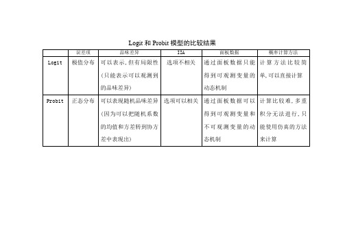
误差项
品味差异
IIA
面板数据
概率计算方法
Logit
极值分布
可以表示,但有局限性(只能表示可以观测到的品味差异)
选项不相关
通过面板数据只能得到可观测变量的动态机制
计算方法比较简单,可以直接计算
Probit
正态分布
可以表现随机品味差异(因为可以把随机系数的均值和方差转到协方差中表现出)
选项可以相关
通过面板数据可以得到可观测变量和不可观测变量的动态机制
计算比较难,多重积分无法进行,只能使用仿真的方法来计算
离散因变量模型(Logit模型,Probit模型).ppt

yi 0
yi 1
所以似然函数为:
n
L
( F (X i))yi (1 F (X i))1yi
i 1
n
ln L ( yi ln F ( X i ) (1 yi ) ln(1 F ( X i )))
i 1
ln L
n i 1
yi f i Fi
(1
yi
)
fi (1 Fi
)
X
P( yi*
0)
P(
* i
Xi)
1
P(
* i
Xi)
1 F (Xi) F (Xi)
F(t) 1 F(t)
E( yi Xi ) 1 P 0 (1 P) F (Xi)
Y E(Y X )
总体回归模型
样本回归模型
Y F ( XB) yi F ( Xi B) i (i 1, 2......n)
U
1 i
Xi 1
i1
第i个个体选择1的效用
U
0 i
Xi 0
i0
第i个个体不选择1(选择0)的效用
U
1 i
U
0 i
Xi (1
0 )
(i1
i0 )
yi* Xi
i
yi 1( yi 0) 选择1
yi
0( yi
0)
不选择1 (选择0)
(二) 二元选择的经济计量一般模型
P( yi
1
Xi)
模型 yi ( Xi B) i
f
(Z )
F'(Z)
eZ (1 eZ )2
(Z )(1 (Z ))
线性化 pi ( Xi B)
∵
(
Z
170-演示文稿-线性概率模型、Logit模型与Probit模型的比较

尽管线性概率模型有明显的不足,但当 解释变量的观察值中没有极端值时 ( 是 指那些能够使得 Y=1 的概率超出 0 ~ 1 区间的解释变量值,可回过去看看 10.2 中的例子 ) ,使用线性概率模型常常能 得到总体回归函数的较好近似。
《计量经济学》,高教出版社, 2011 年 6 月,王少平、杨继生、欧阳志刚等编著
§10.5 线性概率模型、 Logit 模型与 Probit 模型的比较
• 共同点:线性概率模型、 Logit 模型和 Probit 模型都仅是未知的总体回归模型 E(Y|X)=p(Y=1|X) 的近似
• 不同点:线性概率模型的应用及解释相对较简 单和方便,但它不能描述真实总体回归函数的 非线性,也不能将 Y=1 的概率限制在 0 ~ 1 之 间; Logit 模型和 Probit 模型虽然可以从概率 上描述总体回归函数的非线性,从而将 Y=1 的 概率限制在 0 ~ 1 之间,但模型的估计和回归 系数的解释相对更为困难。
《计量经济学》,高教出版社, 2011 年 6 月,王少平、杨继生、欧阳志刚等编著
• Logit 模型和 Probit 模型的比较: 逻辑分布有相对较平坦的尾部,也就是 说, Logit 的条件概率比 Probit 以更慢 的速度趋近于 0 和 1 。但由于 Logit 使用 相对简单的数学形式,因此,实践中常 常选用它。
比较logit 模型和probit 模型
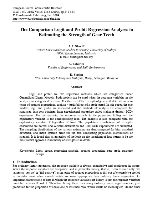
European Journal of Scientific ResearchISSN 1450-216X Vol.27 No.4 (2009), pp.548-553© EuroJournals Publishing, Inc. 2009/ejsr.htmThe Comparison Logit and Probit Regression Analyses inEstimating the Strength of Gear TeethA.A. ShariffCentre For Foundation Studies In Science, University of Malaya50603 Kuala Lumpur, MalaysiaE-mail: asma@.myA. ZaharimFaculty of Engineering and Built EnvironmentK. SopianSERI University Kebangsaan Malaysia, Bangi, Selangor, MalaysiaAbstractLogit and probit are two regression methods which are categorised under Generalized Linear Models. Both models can be used when the response variables in theanalyses are categorical in nature. For the case of the strength of gear teeth data, it can be interms of counted proportions, such as r teeth fail out of n teeth tested. In this paper, the twomodels, logit and probit are discussed and the methods of analysis are compared forsimulated data sets obtained from experimental procedure called staircase design (SCD)experiment. For the analysis, the response variable is the proportion failing and theexplanatory variable is the corresponding load. The analysis is also compared with theexplanatory variable of logarithm of load. The population distributions of strengthsconsidered are normal and Weibull distribution and 1000 SCD experiments are simulated.The sampling distributions of the various estimators are then compared for bias, standarddeviation, and mean squared error for the two contrasting population distributions ofstrength. It is found that, a regression of the logit on the logarithm of load seems to be themost robust approach if normality of strengths is in doubt.Keywords:Logit, probit, regression analysis, counted proportion, gear teeth, staircase design.1. IntroductionFor ordinary linear regression, the response variable is always quantitative and continuous in nature. When the response variables are categorical and in particular binary, that is, it can assume only two values (a ‘yes-no’ or ‘fail-survive’) or in terms of counted proportions (r fail out of n tested) we are led to consider some other models which are more appropriate than ordinary linear regression. An important characteristic of data in which the response variables are binary is that the response variables must lie between 0 and 1. Therefore fitting these data using ordinary linear regression can give prediction for the proportion of above one or less than zero, which would be meaningless. On the otherThe Comparison Logit and Probit Regression Analyses in Estimating the Strength of Gear Teeth 549hand what we actually need in this situation is a regression model which will predict the proportion ofoccurrences, p (let us call them p instead of y ) at certain levels of x .For this type of data, in particular, when the response variables are in terms of countedproportions, the relationship between response variables p and explanatory variables x is a non-linearcurved relationship (S-shaped) curve which is usually called sigmoid . The S-shaped behaviour is verycommon in modeling binomial responses as a function of predictors and also makes use of theassumption that the responses are from underlying binomial or binary distribution. The purpose oflogistic modelling (and also probit) is the same as other modelling techniques used in statistics, that is,to find a model that fits the data best and is the simplest, yet physically reasonable in describing therelationship between the response and the explanatory variables [1]. There is little to distinguishbetween logit and probit models. Both curves are so similar as to yield essentially identical results. Itwas found that probit and logit analysis applied to the same set of data produce coefficient estimateswhich differ approximately by a factor of proportionality, and that factor should be about 1.8 [2].2. Materials and Methods2.1. Logit Versus Probit Regression Techniques Logit model can be presented asp Z Z =+exp()exp()1 (1) where p is the proportion of occurrences, Z =βββ011+++x x k k ... and x x k 1... are the explanatory variables. The inverse relation of equation (1) isZ p p =−⎛⎝⎜⎞⎠⎟ln 1 (2) that is, the natural logarithm of the odds ratio, known as the logit. It transforms p which is restricted tothe range [0, 1] to a range [,]−∞∞ .Probit regression analysis involves modeling the response function with the normal cumulativedistribution function. The probit of a proportion p is just the point on a normal curve with mean 0 andstandard deviation 1 which has this proportion to the left of it.The model can be presented asΦ−==+++1011()...p Z x x k k βββ (3) where p is the proportion and Φ−1 is the inverse of the cumulative distribution function of the standard normal distribution. That is,p Z u du Z ==−−∞∫Φ()exp(/)1222π (4) is the cumulative distribution function of the standard normal distribution.For logistic and probit regression, the binomial, rather than the normal distribution describesthe distribution of the errors and will be the statistic upon which the analysis is based. The principlesthat are used for ordinary linear regression analysis could be adapted to fit both regressions. However,instead of using least square method to fit the model, for logistic and probit regressions, it is moreappropriate to use maximum likelihood estimate. The likelihood function is given asL p p i r i mi n r i i i =−=−∏()11,where the p i are defined in terms of the parameters ββ0,...,k and the known values of the predictorvariables. This has to be maximized with respect to the parameters.550A. A. Shariff, A. Zaharim and K. Sopian2.2. Experimental Design Gear teeth are commonly tested by applying oscillatory loads, using a special machine called pulsator-test machine. In the experiment, the test specimen, in this case the gear tooth is subjected to vibrations of a resonant spring/mass system. When this happens, it experiences stresses and crack propagation takes place. Eventually, after certain number of cycles the tooth fails. The number of cycles to failure can then be recorded. If the tooth does not fail after a certain fixed number of cycles, it is considered to have survived in the experiment. The experimental procedure used is the well-known staircase design (SCD). SCD experiment is also known as sensitivity testing or ‘up-and-down’ method [3] where the testing of specimens is made close to the anticipated mean level. In the experiment the first test piece should be tested at a load level assumed to be near the mean value of the fatigue strength. If failure occurs before N cycles, the next test piece is tested at one step, a fixed change in load, below the first load level. Otherwise, the next test at the load one step above the first level. This procedure is continued until all the pieces have been tested. The increment between load levels should be equal for steps up and down and should be approximately one standard deviation of the fatigue strength distribution. Since the data obtained are categorical in nature, particularly in terms of counted proportions, fatigue strength of a gear is then determined by analysing the data obtained using appropriate statistical techniques, in this case logit and probit.2.3. Analysis For SCDThe results obtained in the experiment are then analysed using logit and compared with probit. Thelogit transformation of p is defined by ln(p p1−, and the lines ln()p px 101−=+ββ are fitted, using maximum likelihood. A comparison is made with fitting the line,ln()ln p px 101−=+ββ which is equivalent to assuming a log-normal distribution of strengths.For probit, results of SCD experiment are analysed by fitting the lineΦ−=+101()p x ββwhere p is the proportion failing and x is the corresponding load. This is equivalent to assuming a normal distribution of strengths. Then a comparison is made withΦ−=+101()ln p x ββThe estimated mean fatigue strength, μ, and the lower 1% point of the distribution of fatiguestrength, .x 099, are the values of x corresponding to p =05. and p =001. respectively. The standarddeviation can be estimated from ( )/..σμ=−x 099233 .The methods of analysis have been compared for simulated data sets. The population distribution of strengths is specified and 1000 SCD experiments are simulated. The sampling distributions of the various estimators can thus be compared for bias, standard deviation, and mean squared error. Two contrasting population distributions of strength are considered:(i). normal distribution with mean of 20.0 and standard deviation of 2.0;(ii).W eibull distribution [4 – 6], which has a cumulative distribution function F(x) defined by Pr()()exp[(/)]X x F x x b c <==−−1),with shape parameter, c = 2, and scale parameter, b = 22.56. These parameter values correspond to a mean of 20 and standard deviation of 10.45. The probability density functions of both distributions are plotted in Figure 1. The Weibull distribution has a substantial area near zero. This might be realistic forThe Comparison Logit and Probit Regression Analyses in Estimating the Strength of Gear Teeth 551the strength of a component being tested under extreme conditions, as in an accelerated testing programme. It could also be interpreted as strength above some minimum value.Figure 2: Probability density function of normal (,.)μσ==2020 and Weibull (,.45)μσ==2010distributionIn the simulation, each SCD used 50 test specimens. There are 1000 independent SCD experiments within a simulation. Each specimen put on test is randomly selected from the 50 specimens. For the normal distribution the load increment is chosen to be 2, while for the Weibull distribution it is chosen to be 6, since the standard deviation for this distribution is larger.Results obtained from the above experiments are analysed using logit and then compared with probit analyses for each distribution. The means and standard deviations of the estimated mean, standard deviation and lower 1% point of the strength distribution are computed from 1000 SCD experiments for each distribution.These results are tabulated in Table 1; the standard deviations of these statistics are shown in brackets, and the root mean square error (RMSE) is also calculated using the formula552A. A. Shariff, A. Zaharim and K. Sopian Table 1:Results of Staircase Experiments Analysed by Probit and Logit Regression Techniques with the load on a linear scale for Each Distribution.RMSE (standard deviation)(bias)22=+where, bias = (actual value - mean of estimated value).These RMSE values are presented in square brackets. Table 2 shows results for the logit and probit analysis using a logarithmic scale for load.Table 2: Results of Staircase Experiments Analysed by Probit and Logit Regression Techniques with the loadon a logarithmic scale for Each DistributionThe Comparison Logit and Probit Regression Analyses in Estimating the Strength of Gear Teeth 553 3. Results and DiscussionTable 1 indicates that for load on linear scale, results obtained by probit analysis are more realistic with less error as compared to logit for normal distribution of strength. Logit analysis appears to overestimate the standard deviation and hence underestimate the lower one percent point of the distribution. However, for the Weibull distribution, which has a large standard deviation, both methods predict negative lower 1% points which are physically impossible.Regressing the sample probit against the logarithm of load (refer to Table 2) gives estimates with a smaller standard deviation and, somewhat surprisingly, a slightly smaller mean squared error. Regressing logit of the sample proportion against the logarithm of load is a slight improvement on the probit analysis and aconsiderable improvement on a regression of logit against load.When sampling from both normal and Weibull distributions the regression of the logit against the logarithm of load gives an estimate of the lower 1% point with the smallest mean squared error. Overall, a regression of the logit on the logarithm of load seems to be the most robust approach if normality of strengths is in doubt.References[1]Hosmer, D.W., & Lemeshow, S. (1989). Applied Logistic Regression. Wiley Series inProbability and Mathematical Science. Wiley-Interscience Publication.[2]Aldrich, J.H. & Nelson, F.D. (1984). Linear Probability, Logit and Probit Models. SageUniversity Paper series on Quantitative Applications in the Social Sciences, 07-045. Beverly Hills and London: Sage Pubns.[3]Lloyd, D. K., & Lipow, M. (1989). Reliability: managements, methods, and mathematics(Second ed.). American Society for Quality Control.[4]ISO/CD 12107. (1997). Draft for Public Comment, Metallic Materials - Fatigue Testing -Statistical Planning and Analysis of Data, British Standard Institution.[5]Weibull, W. (1961). Fatigue Testing and the Analysis of Results. Pergamon Press. Oxford.[6]Crowder, M.J., Kimber, A.C., Smith, R.L. & Sweeting, T.J. (1991). Statistical Analysis ofReliability Data. Chapman and Hall.。
Probit回归模型
Probit回归模型
Probit模型也是一种广义的线性模型,当因变量为分类变量时,有四种常用的分析模型:
1.线性概率模型(LPM)
2.Logistic模型
3.Probit模型
4.对数线性模型
和Logistic回归一样,Probit回归也分为:二分类Probit 回归、有序多分类Probit回归、无序多分类Probit回归。
我们再来回顾一下因变量为分类变量的分析思路,以二分类因变量为例,为例使y的预测值在[0,1]之间,我们构造一个理论模型:
函数F(x,β)被称为“连接函数”,如果连接函数为标准正态分布,则模型称为Probit回归模型,如果连接函数为logistic 分布,则模型称为logistic回归模型。
Probit回归也是利用最大似然法进行参数估计,且估计过程和Logistic一样。
Probit回归Logistic回归都属于离散因变量分析模型,二者没有本质区别,通常情况下可以互换使用,而且函数图像几乎重叠,只是反映的意义不同。
然而Logistic 回归的应用比Probit回归广泛得多,这主要是因为Logistic回
归的偏回归系数解释起来更加直观和易于理解——Probit回归的偏回归系数含义为其他自变量保持不变的时该自变量每增加一个单位,出现某个结果的概率密度函数的改变值,这很难以理解。
那么什么情况下能够使用Probit回归替代Logistic回归呢?可从以下两个方面考虑
1.自变量中连续型变量较多
2.残差符合正态分布。
probit logit 解析表达式 -回复
probit logit 解析表达式-回复Probit和Logit是统计学中广泛使用的两种回归模型形式,常用于预测二分类的离散变量。
在本文中,我们将详细解析Probit和Logit模型,并解释它们在实际应用中的意义和优缺点。
首先,让我们简要介绍一下Probit和Logit模型。
它们都是广义线性模型的一种形式,用于估计二分类变量的概率。
具体而言,Probit模型使用标准正态分布的累积分布函数作为链接函数,而Logit模型使用逻辑函数(即S形函数)作为链接函数。
下面我们将以步骤的形式逐一解析这两个模型。
步骤一:建立基本假设在使用Probit或Logit模型之前,我们首先需要明确一些基本假设。
首先,我们假设因变量服从二项分布(或二分类变量的概率)。
其次,我们假设自变量与因变量之间存在线性关系,即可以用一个线性方程的形式表示。
步骤二:设定模型形式为了使用Probit或Logit模型,我们需要设定一个适当的模型形式。
具体而言,我们假设因变量的概率是自变量的线性组合经过链接函数的变换后的结果。
对于Probit模型而言,我们的设定如下:P(y=1 x) = Φ(x'β),其中Φ表示标准正态分布的累积分布函数。
对于Logit模型而言,我们的设定如下:P(y=1 x) = 1 / (1 + exp(-x'β)),其中exp表示指数函数。
步骤三:估计参数为了估计Probit或Logit模型的参数,我们使用最大似然估计方法。
简言之,我们希望找到一组参数,使得给定自变量后,模型预测的因变量概率最大。
在实际应用中,我们通过最大似然估计方法,求解出模型中的参数。
这些参数可以在一定程度上解释自变量对因变量的影响。
步骤四:解释结果最后,我们可以通过估计得到的参数来解释模型的结果。
在Probit和Logit 模型中,参数的正负符号以及显著性水平可以告诉我们自变量与因变量之间的关系。
需要注意的是,Probit和Logit模型都是非线性回归模型,因此参数的解释并不像传统的线性回归模型那样直观。
离散因变量模型(Logit 模型,Probit模型)

yi F ( X i B) i
eZ F(Z) 1 eZ (Z)
模型 yi ( Xi B) i
f
(Z)
F'(Z)
eZ (1 eZ )2
(Z )(1 (Z ))
线性化 pi ( Xi B)
∵
(Z )
eZ 1 eZ
pi ( X i B) eXiB 1 pi 1 ( X i B)
LPM, Probit, Logit
1、 线性概率模型(LPM)
如果选择 F ( XiB) XiB yi X i B i
E( yi Xi ) E( Xi B i ) Xi B yi E( yi X i ) i
P( yi 1 X i ) pi
P( yi 0 Xi ) 1 pi
i 1
ln L
n i 1
yi f i Fi
(1
yi
)
fi (1 Fi
)
X
i
0
求驻点即可。
三、 二元选择模型的显著性检验
1. t 检验 (大样本下用正态分布)
2. 准R2
Pseudo R 2 1 log Lur log Lr
3. 线性约束F检验
0.052 0.873 0.052
-.0050766 -6.326276
-486.509
1.359199 5.373068 1.593967
(3)得到估计式: 注:括号里是p值。
ln( 1
p
p
)
242.4576
0.6771Score
0.4766D1
解释概率模型:Logit,Probit以及其他广义线性模型

[6.2]
37
在使用多类别logit模型时,一个重要的问
等式6.1和等式6.2可以推出如下:
题就是在无关选择之间独立性的假设,或者称
做IIA。简单来说,IIA的特性明确了每任意两
个选择(回答类别)的概率的比例都不应系统性 地受到其他任何选择的影响。这是一个非常重
多类别logit的关系函数:
察到的和估计出来的两者之间的比数比的差就会消失。
10
给定自变量后的预测概率
这些预测的概率告诉我们每一组里面有多少成员有过性行为,给出了一个简单、直观的理 解。基于logit 模型,预测大约55%的黑人男性有过性行为,白人女性青少年有过性行为仅为大
约15%。
11
发生某事件概率的边际效应
我们去看解释变量对发生某事件的概率所带来的边际效应。可以用下面的等式来表示:
35
发生某事件概率的边际效应
对事件概率的边际效应: 利用上面的公式我们可以得到在这个例子中的边 际效应如右图所示可以看出:AFQT得分,用偏导数 和用预测概率差两个方法都能给出基本相同的结果。 (AFQT是连续变量);如果计算入伍时的婚姻状况 可以看出,用两种方法计算出被分配到高级任务的概 率减少了大约相差5%。(入伍时的婚姻状况是二元变 量)在有二分自变量的时候,使用偏导数的方法产生
确的值其实是在这两个值之间或接近这两个值。
在一些特殊情况logit和probit模型得出的估计是差得非常远的,这样就一定要去考虑使用最
合适的模型了。对于尾端比重很大的分布来说,我们更应该考虑logit模型。
16
四、序列logit和probit模型
有时,一些因变量的结果是多样的,但它们并不是一些完全离散的毫无关联的类别。这些反应的类 别可以看做一系列阶段。晚期的响应是嵌套在早期的响应里面的。例如,结婚的决定是分两个阶段的: 一个人是否计划结婚,然后就是这个婚姻是否会在结束了某种教育程度之前开始(例如完成高中或者大 学学历)。
李子奈《计量经济学》考试试卷(77)

某财经学院李子奈《计量经济学》课程试卷(含答案)__________学年第___学期考试类型:(闭卷)考试考试时间:90 分钟年级专业_____________学号_____________ 姓名_____________1、判断题(3分,每题1分)1. 差分平稳过程与趋势平稳过程相比,更适宜于长期预测。
()正确错误答案:错误解析:趋势平稳过程代表了一个时间序列长期稳定的变化过程,因而与差分平稳过程相比,更适宜于长期预测。
2. 宏观经济决策方式主要分为以集中决策为主和以分散决策为主两类。
前者是市场经济体制的重要体现,后者则是计划经济体制的主要反映。
()正确错误答案:错误解析:宏观经济决策方式主要分为以集中决策为主和以分散决策为主两类。
前者是计划经济体制的重要体现,后者则是市场经济体制的主要反映。
3. 总体回归函数给出了对应于每个自变量的因变量的值。
()正确错误答案:错误解析:总体回归函数给出了对应于每个自变量的被解释变量的均值。
2、名词题(5分,每题5分)1. t检验答案:t检验是针对每个解释变量进行的显著性检验,即构造一个t统计量,如果该统计量的值落在置信区间外,就拒绝原假设。
t检验主要用于样本含量较小(例如n<30),总体标准差σ未知的正态分布资料。
t检验分为单总体检验和双总体检验。
单总体t检验时检验一个样本平均数与一个已知的总体平均数的差异是否显著。
当总体分布是正态分布,如总体标准差未知且样本容量小于30,那么样本平均数与总体平均数的离差统计量呈t分布。
双总体t检验是检验两个样本平均数与其各自所代表的总体的差异是否显著。
双总体t检验又分为两种情况,一是独立样本t检验,一是配对样本t检验。
解析:空3、简答题(25分,每题5分)1. 假设居民户储蓄(Y)与收入(X)之间可建立如下形式的储蓄模型Y=β0+β1X+μ,。
其中,ε为具有零均值E(δ)=0、同方差Var(ε)=σε2且与X 相互独立的随机变量。
logit 和probit模型的系数解释
logit 和probit模型的系数解释Logit和Probit模型是通常在二分类问题中使用的统计模型,这些模型的系数表示了解释变量对于被解释变量的影响程度。
在本文中,我将解释Logit和Probit模型的系数含义,并探讨它们在实际应用中的解释。
首先,我们先来了解一下Logit和Probit模型。
这两种模型都属于广义线性模型(Generalized Linear Models,简称GLM),使用类似的数学形式来描述被解释变量与解释变量之间的关系。
对于一个二分类问题,我们希望找到一个函数f(x)来预测被解释变量y=1的概率P(y=1|x),其中x表示解释变量。
Logit模型将被解释变量与解释变量的关系建模为一个logistic函数,它的数学形式是:P(y=1|x) = 1 / (1 + exp(-z))其中,z = β0 + β1*x1 + β2*x2 + ... + βn*xn表示线性预测器,β0,β1,...,βn表示系数。
这些系数可以表示是模型的"回归系数",它们衡量了解释变量在对被解释变量的影响程度上的贡献。
Logit模型中的系数解释是基于"对数几率比"(log odds ratio)的改变来描述的。
具体来说,系数β1的解释是:当其他解释变量保持不变时,若解释变量x1的值增加一个单位,则被解释变量y=1的对数几率(即log odds)将增加β1个单位。
换句话说,系数β1表示了解释变量x1对于预测y=1的概率的影响程度。
如果β1是正的,表示x1的增加会增加预测y=1的概率,而如果β1是负的,则表示x1的增加会减少预测y=1的概率。
Probit模型的数学表达形式与Logit模型略有不同,它使用了标准正态分布的累积分布函数(CDF)来建模被解释变量与解释变量之间的关系:P(y=1|x) = Φ(z)其中,Φ(z)表示标准正态分布的累积分布函数,z的计算方式与Logit模型相同。
logit 和probit模型的系数解释 -回复
logit 和probit模型的系数解释-回复【logit 和probit 模型的系数解释】1. 引言在统计学和经济学中,logit模型和probit模型是两种常见的二元选择模型,它们被广泛应用于解释和预测离散选择的行为。
本文将详细介绍logit 和probit模型的系数解释步骤,并对其应用领域和优缺点进行讨论。
2. 模型背景logit模型和probit模型是建立在二元选择数据上的概率模型。
在这两种模型中,我们假设个体i选择某个选项的概率是一个关于自变量X的非线性函数F(X)的模型,其中F(X)是一个累积分布函数(CDF)。
logit模型和probit模型是两种常见的CDF函数选择,分别使用逻辑函数(logistic function)和正态分布函数(normal distribution function)进行建模。
3. logit模型的系数解释logit模型的系数解释可以通过观察变量系数的大小、正负以及显著性水平来进行。
首先,系数的大小可以表示预测变量在选择行为中的影响程度。
一个正的系数表示该变量与选择行为正相关,即该变量的增加会增加选择某个选项的概率。
一个负的系数表示该变量与选择行为负相关,即该变量的增加会降低选择某个选项的概率。
其次,系数的正负可以表明变量对选择行为的方向性影响。
最后,统计显著性测试可以帮助我们确定该系数是否显著不等于零,即该变量对选择行为的影响是否存在。
4. probit模型的系数解释probit模型的系数解释与logit模型类似。
同样,我们可以通过观察变量系数的大小、正负以及显著性水平来解释系数。
不同的是,probit模型中的系数解释基于正态分布函数的特性。
具体而言,一个正的系数表示该变量的增加会使选择某个选项的概率上升,并且该上升符合正态分布函数的曲线形状。
一个负的系数则说明选择行为概率会下降。
同样,系数的正负可以揭示变量对选择行为的方向性影响。
最后,显著性测试也可以用来确认系数的显著性。
probit logit 解析表达式
probit logit 解析表达式(最新版)目录1.介绍 Probit 和 Logit 模型2.解析 Probit 和 Logit 模型的表达式3.比较 Probit 和 Logit 模型的异同正文Probit 和 Logit 模型是两种常用的概率回归模型,常用于处理二元变量的预测问题。
在这两种模型中,我们都需要解析它们的表达式,以便更好地理解模型的预测机制。
首先,我们来看 Probit 模型。
Probit 模型是一种用于二元响应变量预测的线性模型。
它的表达式可以解析为:Probit(Y=1|X=x) = Φ(β0 + β1X1 + β2X2 +...+ βnXn)其中,Y 代表二元响应变量,X 代表自变量,β0、β1、β2 等为模型参数,Φ为标准正态分布函数的逆函数。
接着,我们看 Logit 模型。
Logit 模型也是一种用于二元响应变量预测的线性模型。
它的表达式可以解析为:Logit(Y=1|X=x) = ln(π1 / π0) = β0 + β1X1 + β2X2 +...+ βnXn其中,Y 代表二元响应变量,X 代表自变量,β0、β1、β2 等为模型参数,π0 和π1 分别为两个类别的概率。
通过比较 Probit 和 Logit 模型的表达式,我们可以发现两者的主要区别在于概率计算的方式。
Probit 模型使用的是标准正态分布函数的逆函数,而 Logit 模型则使用的是对数函数。
此外,Probit 模型的截距项为β0,而 Logit 模型的截距项为 ln(π1 / π0)。
总的来说,Probit 和 Logit 模型都是用于解决二元变量预测问题的有效工具。
比较线性模型和Probit模型、Logit模型
研究生考试录取相关因素的实验报告一,研究目的通过对南开大学国际经济研究所1999级研究生考试分数及录取情况的研究,引入录取与未录取这一虚拟变量,比较线性概率模型与Probit模型,Logit模型,预测正确率。
二,模型设定表1,南开大学国际经济研究所1999级研究生考试分数及录取情况见数据表定义变量SCORE :考生考试分数;Y :考生录取为1,未录取为0。
上图为样本观测值。
1. 线性概率模型 根据上面资料建立模型i i i SCORE B B Y μ++=*21用Eviews 得到回归结果如图:Dependent Variable: Y Method: Least Squares Date: 12/10/10 Time: 20:38Sample: 1 97Included observations: 97VariableCoefficientStd. Error t-Statistic Prob.C -0.847407 0.159663 -5.307476 0.0000 SCORE0.0032970.0005216.3259700.0000R-squared0.296390 Mean dependent var 0.144330 Adjusted R-squared 0.288983 S.D. dependent var 0.353250 S.E. of regression 0.297866 Akaike info criterion 0.436060 Sum squared resid 8.428818 Schwarz criterion 0.489147 Log likelihood -19.14890 F-statistic 40.01790 Durbin-Watson stat0.359992 Prob(F-statistic) 0.000000参数估计结果为: iY ˆ-0.847407+0.003297 i SCORESe=(0.159663)( 0.000521) t=(-5.307476) (6.325970) p=(0.0000) (0.0000)预测正确率:Forecast: YF Actual: YForecast sample: 1 97Included observations: 97Root Mean Squared Error0.294780Mean Absolute Error 0.233437Mean Absolute Percentage Error8.689503Theil Inequality Coefficient 0.475786Bias Proportion 0.000000Variance Proportion 0.294987Covariance Proportion 0.7050132.Logit模型Dependent Variable: YMethod: ML - Binary Logit (Quadratic hill climbing) Date: 12/10/10 Time: 21:38Sample: 1 97Included observations: 97Convergence achieved after 11 iterations Covariance matrix computed using second derivativesVariable Coefficient Std. Error z-Statistic Prob.C-243.7362125.5564-1.9412480.0522SCORE0.679441 0.350492 1.938536 0.0526Mean dependent var 0.144330 S.D. dependent var 0.353250 S.E. of regression 0.115440 Akaike info criterion 0.123553 Sum squared resid 1.266017 Schwarz criterion 0.176640 Log likelihood -3.992330 Hannan-Quinn criter. 0.145019 Restr. log likelihood -40.03639 Avg. log likelihood -0.041158 LR statistic (1 df) 72.08812 McFadden R-squared 0.900282Probability(LR stat) 0.000000Obs with Dep=0 83 Total obs 97Obs with Dep=114得Logit 模型估计结果如下p i = F (y i ) =)6794.07362.243(11i x e +--+ 拐点坐标 (358.7, 0.5)其中Y=-243.7362+0.6794X预测正确率Forecast: YF Actual: YForecast sample: 1 97 Included observations: 97Root Mean Squared Error 0.114244 Mean Absolute Error0.025502Mean Absolute Percentage Error 1.275122Theil Inequality Coefficient 0.153748Bias Proportion 0.000000Variance Proportion 0.025338Covariance Proportion 0.9746623.Probit模型Dependent Variable: YMethod: ML - Binary Probit (Quadratic hill climbing) Date: 12/10/10 Time: 21:40Sample: 1 97Included observations: 97Convergence achieved after 11 iterations Covariance matrix computed using second derivativesVariable Coefficient Std. Error z-Statistic Prob.C-144.456070.19809-2.0578330.0396SCORE0.4028680.196186 2.0535040.0400 Mean dependent var0.144330 S.D. dependent var0.353250 S.E. of regression0.116277 Akaike info criterion0.122406 Sum squared resid 1.284441 Schwarz criterion0.175493Log likelihood-3.936702 Hannan-Quinn criter.0.143872 Restr. log likelihood-40.03639 Avg. log likelihood-0.040585LR statistic (1 df)72.19938 McFadden R-squared0.901672 Probability(LR stat)0.000000Obs with Dep=083 Total obs97Obs with Dep=114Probit模型最终估计结果是p i = F(y i) = F (-144.456 + 0.4029 x i) 拐点坐标(358.5, 0.5)预测正确率Forecast: YFActual: YForecast sample: 1 97Included observations: 97Root Mean Squared Error0.115072Mean Absolute Error 0.025387Mean Absolute Percentage Error 1.216791Theil Inequality Coefficient 0.154476Bias Proportion 0.000084Variance Proportion 0.020837Covariance Proportion 0.979080预测正确率结论:线性概率模型RMSE=0.294780 MAE=0.233437 MAPE=8.689503Logit模型RMSE=0.114244 MAE=0.025502 MAPE=1.275122Probit模型RMSE=0.115072 MAE=0.025387 MAPE=1.216791由上面结果可知线性概率模型的RMSE、MAE、MAPE 均远远大于Logit模型和Probit模型,说明其误差率比Logit模型和Probit模型大很多,所以正确率远远小于Logit模型和Probit模型。
- 1、下载文档前请自行甄别文档内容的完整性,平台不提供额外的编辑、内容补充、找答案等附加服务。
- 2、"仅部分预览"的文档,不可在线预览部分如存在完整性等问题,可反馈申请退款(可完整预览的文档不适用该条件!)。
- 3、如文档侵犯您的权益,请联系客服反馈,我们会尽快为您处理(人工客服工作时间:9:00-18:30)。
研究生考试录取相关因素的实验报告
一,研究目的
通过对南开大学国际经济研究所1999级研究生考试分数及录取情况的研究,引入录取与未录取这一虚拟变量,比较线性概率模型与Probit模型,Logit模型,预测正确率。
二,模型设定
表1,南开大学国际经济研究所1999级研究生考试分数及录取情况见数据表
定义变量SCORE :考生考试分数;Y :考生录取为1,未录取为0。
上图为样本观测值。
1. 线性概率模型
根据上面资料建立模型
i i
i SCORE
B B Y μ++=*21
用Eviews 得到回归结果如图:
Dependent Variable: Y Method: Least Squares Date: 12/10/10 Time: 20:38
Sample: 1 97
Included observations: 97
Variable
Coefficient Std. Error t-Statistic Prob. C -0.847407 0.159663 -5.307476 0.0000 SCORE
0.003297
0.000521
6.325970
0.0000
R-squared 0.296390 Mean dependent var 0.144330 Adjusted R-squared 0.288983 S.D. dependent var 0.353250 S.E. of regression 0.297866 Akaike info criterion 0.436060 Sum squared resid 8.428818 Schwarz criterion 0.489147 Log likelihood -19.14890 F-statistic 40.01790 Durbin-Watson stat
0.359992 Prob(F-statistic)
0.000000
参数估计结果为:i
Y ˆ-0.847407+0.003297 i
SCORE
Se=(0.159663)( 0.000521)
t=(-5.307476) (6.325970)
p=(0.0000) (0.0000)
预测正确率:
Forecast: YF Actual: Y
Forecast sample: 1 97 Included observations: 97 Root Mean Squared Error 0.294780 Mean Absolute Error
0.233437 Mean Absolute Percentage Error 8.689503 Theil Inequality Coefficient 0.475786 Bias Proportion 0.000000 Variance Proportion 0.294987 Covariance Proportion
0.705013
2.Logit 模型
Dependent Variable: Y
Method: ML - Binary Logit (Quadratic hill climbing) Date: 12/10/10 Time: 21:38
Sample: 1 97
Included observations: 97
Convergence achieved after 11 iterations
Covariance matrix computed using second derivatives
Variable
Coefficient Std. Error z-Statistic Prob. C -243.7362 125.5564 -1.941248 0.0522 SCORE
0.679441
0.350492
1.938536
0.0526 Mean dependent var 0.144330 S.D. dependent var 0.353250 S.E. of regression 0.115440 Akaike info criterion 0.123553 Sum squared resid 1.266017 Schwarz criterion 0.176640 Log likelihood -3.992330 Hannan-Quinn criter. 0.145019 Restr. log likelihood -40.03639 Avg. log likelihood -0.041158 LR statistic (1 df) 72.08812 McFadden R-squared 0.900282
Probability(LR stat) 0.000000
Obs with Dep=0 83 Total obs 97
Obs with Dep=1
14
得Logit 模型估计结果如下
p i = F (y i ) =
)
6794.07362.243(11
i x e
+--+ 拐点坐标 (358.7, 0.5)
其中Y=-243.7362+0.6794X
预测正确率
Forecast: YF Actual: Y
Forecast sample: 1 97 Included observations: 97 Root Mean Squared Error 0.114244 Mean Absolute Error
0.025502 Mean Absolute Percentage Error 1.275122 Theil Inequality Coefficient 0.153748 Bias Proportion 0.000000 Variance Proportion 0.025338 Covariance Proportion
0.974662
3.Probit 模型
Dependent Variable: Y
Method: ML - Binary Probit (Quadratic hill climbing) Date: 12/10/10 Time: 21:40
Sample: 1 97
Included observations: 97
Convergence achieved after 11 iterations
Covariance matrix computed using second derivatives
Variable
Coefficient Std. Error z-Statistic Prob. C -144.4560 70.19809 -2.057833 0.0396 SCORE
0.402868
0.196186
2.053504
0.0400 Mean dependent var 0.144330 S.D. dependent var 0.353250 S.E. of regression 0.116277 Akaike info criterion 0.122406 Sum squared resid 1.284441 Schwarz criterion 0.175493 Log likelihood -3.936702 Hannan-Quinn criter. 0.143872 Restr. log likelihood -40.03639 Avg. log likelihood -0.040585 LR statistic (1 df) 72.19938 McFadden R-squared 0.901672
Probability(LR stat) 0.000000
Obs with Dep=0 83 Total obs 97
Obs with Dep=1
14
Probit模型最终估计结果是
p i = F(y i) = F (-144.456 + 0.4029 x i) 拐点坐标(358.5, 0.5)
预测正确率
Forecast: YF
Actual: Y
Forecast sample: 1 97
Included observations: 97
Root Mean Squared Error 0.115072
Mean Absolute Error 0.025387
Mean Absolute Percentage Error 1.216791
Theil Inequality Coefficient 0.154476
Bias Proportion 0.000084
Variance Proportion 0.020837
Covariance Proportion 0.979080
预测正确率结论:线性概率模型RMSE=0.294780 MAE=0.233437 MAPE=8.689503 Logit模型 RMSE=0.114244 MAE=0.025502 MAPE=1.275122 Probit模型 RMSE=0.115072 MAE=0.025387 MAPE=1.216791 由上面结果可知线性概率模型的RMSE、MAE、MAPE 均远远大于Logit模型和Probit模型,说明其误差率比Logit模型和Probit模型大很多,所以正确率远远小于Logit模型和Probit模型。
而Logit模型和Probit模型的RMSE、MAE、MAPE相差很小,所以正确率相差不大。
综上所诉,此数据可以用Logit模型和Probit模型代替线性概率模型进行分析。