ASPEN换热过程
ASPEN换热过程PPT课件

31 Introduction to Aspen Plus
▪ 传热膜系数 ( Film coefficients )
▪ 用户子程序 ( User-subroutine )
28 Introduction to Aspen Plus
管壳式换热器结构名称
单程管壳式换热器 1 —外壳 2—管束 3、4—接管 5—封头
6—管板 7—折流板
29 Introduction to Aspen Plus
HeatX—U-相态法
26 Introduction to Aspen Plus
HeatX—应用示例(1)
❖ 用1200kg/hr饱和水蒸汽(0.3MPa)加热2000kg/hr甲醇 (20℃、0.3MPa)。离开换热器的蒸汽冷凝水压力为 0.28MPa、过冷度为2℃。换热器传热系数根据相态 选择。求甲醇出口温度、相态、需要的换热面积。 (LMTD校正选用0.95)
❖ 冷物流出口过热度
选
(Cold stream outlet degrees superheat) 项
❖ 冷物流出口蒸汽分率
(Cold stream outlet vapor fraction)
22 Introduction to Aspen Plus
HeatX—冷物流出口温差
23 Introduction to Aspen Plus
Aspen Plus 换热过程
Introduction to Aspen
2021/2/23
1
换热器
模型 说明
目的
用法
Heater 加热器或冷却器 确定热和相态条件
换热器、冷却器、阀门、当与功有关 的结果不需要时的泵和压缩机
HeatX 两物流换热器 两股物流的换热器
运用aspen及其套件设计换热器

运用aspen及其套件EDR设计换热器青海大学化工学院张鹏宇目录1.生产要求设定2.启动aspen设置前奏2.1确定合适的modle library 模块2.2建立流程图2.3输入工程标题2.4输入组分2.5选择物性方法2.6输入物流参数3.进行换热器选型3.1采用shortcut简捷计算3.2填写估计的总传热系数3.3模拟计算,列出简捷计算结果3.4按国家标准选型4.选择Detailed详细核算4.1设置冷热流体走程4.2使用Design Specification调整冷却水流率4.3设置壳程管程压降计算方式4.4设置总传热系数计算方式4.5填写冷热流体侧污垢系数4.6填写壳程管程数据4.7填写折流板及管嘴数据4.8运行计算,列出换热器详细计算结果4.8.1 exchanger details换热器详细数据4.8.2 pres drop 各程压力降及压力降分析4.8.3 流速探讨及分析5.用EDR 软件核算,出图5.1 数据传递5.2 EDR数据检查,核对补充5.3运行计算,列出换热器详细计算结果5.3.1 EDR换热器详细数据5.3.2 pres drop 各程压力降及压力降分析5.3.3 流速探讨及分析5.4列出换热器装配图5.5列出换热器布管图和设备数据5.6打印出图6.对比Aspen换热器详细计算,说明EDR其优缺点。
1.生产要求设定某生产过程中,需处理每年114000吨/年苯,现将苯从80度冷却至40度,冷却介质采用循环水。
循环水入口温度32.5度,出口温度取37.5度。
要求换热器裕度为10%~25%,换热器内流体流动阻力小于50Kpa.2.启动ASPEN设置前奏2.1选择合适的modle library 模块启动ASPEN,新打开一个空白的blank文件,该换热器用循环水冷却,冬季操作时进口温度会降低,考虑到这一因素,估计该换热器的管壁温和壳体壁温之差较大,因此初步确定选用带膨胀节的固定管板式换热器。
ASPEN换热器模拟实例教程

Aspen plus换热器模拟概述换热器模块Heater加热器/冷却器确定出口物流的热和相态条件换热器,冷却器,阀门,与功有关的结果不需要时的泵和压缩机HeatX双物流换热器在两个物流之间换热两股物流的换热器当知道几何尺寸时核算管壳式换热器MHeatX 多物流换热器在多股物流之间换热多股热流和冷流换热器两股物流的换热器LNG换热器Hetran管壳式换热器与BJAC 管壳式换热器的接口程序管壳式换热器包括釜式再沸器Aerotran空冷换热器与BJAC 空气冷却换热器的接口程序错流式换热器包括空气冷却器HeatX换热器1.概述HeatX有两种简捷法和严格法计算模型。
简捷法(Shortcut)计算不需要换热器结构或几何尺寸数据,可以使用最少的输入量来模拟一个换热器。
Shortcut模型可进行设计模拟两种计算,其中设计计算依据工艺参数和总传热系数估算出传热面积。
严格法(Detailed)可以用换热器几何尺寸去估算传热膜系数、总传热系数、压降、对数平均温差校正因子等。
严格法核算模型对HeatX提供了较多的规定选项,但也需要较多的输入。
Detailed模型不能进行设计计算。
可以将HeatX 的Shortcut和Detailed结合完成换热器设计计算。
首先依据给定的设计条件用Shortcut 估算传热面积,然后依据Shortcut的计算结果用Detailed 进行核算。
在使用 HeatX 模型前,首先要弄清下面这些问题:(1)HeatX能够模拟的管壳换热器类型逆流和并流换热器;弓形隔板TEMA E, F, G, H, J和X壳换热器;圆形隔板TEMA E和F壳换热器;裸管和翅片管换热器。
(2)HeatX能够进行的计算全区域分析;传热和压降计算;显热、气泡状气化、凝结膜系数计算;内置的或用户定义的关联式。
(3)HeatX不能进行进行的计算机械震动分析计算;估算污垢系数。
(3)Hesttx需要的输入规定必须提供下述规定之一换热器面积或几何尺寸;换热器热负荷;热流或冷流的出口温度;在换热器两端之一处的接近温度;热流或冷流的过热度/过冷度;热流或冷流的气相分率(气相分率为 0 表饱和液相);热流或冷流的温度变化。
aspen导热油换热计算
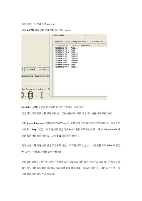
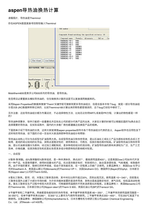
请看图片,导热油是Therminol你在ASPEN里面直接寻找物性输入TherminolMobiltherm600是美孚公司600系列的导热油,是导热油。
我觉得没必要重新去模拟导热油的,仅仅做换热计算的话是可以直接调用数据库的。
采用Aspen Properties的数据库搜索"Therm”关键字即可搜索到更多导热油组分,但是在版本中有个bug,就是一部分导热油组分是从B-JAC数据库转移过来的,比如Therminol-66计算出来的物性都是错误的,这个bug已经在中修好了。
另外注意:这些导热油组分都为专属设定,不必选择物性方法,比如无论你用NRTL或者是PR方程,计算出的物性都是一样的!导热油种类繁多,软件只能把一些最著名并且知名公司的部分代表产品列出来,大家在计算的时候可以根据后面的Tb沸点自己选择需要的导热油,在实际采购中,国内的大多数厂商也都遵循这些典型产品的规律。
下面简单介绍下导热油的分类,这样大家就清楚aspen properties软件中各个导热油组分代表的含义,Aspen软件也没用包含下述所有的导热油,但下面的介绍一定会对大家选择那种导热油组分有帮助:导热油从结构上可分为合成型与矿油型两大类。
合成型导热油又称热传导液,是以石油化工或化工产品为原料经有机合成工艺制得,是纯的或比较纯的化学品,其特点是稳定性好,使用寿命长,可再生,但其价格也相对较高。
矿油型导热油又称热传导油,是以石油某线馏分为原料,经过加工调配制成,是多种烷烃组分的混合物。
矿油型导热油的原料来源较为广泛,生产工艺简单,价格低廉,但其热稳定性和抗氧化性受其多组分物质特性的影响相对较差。
一、合成型①联苯-联苯醚。
由%联苯醚和%联苯组成,是一种共沸体系,沸点257°,最高使用温度400°。
这是美国Dow公司30年代开发的一种产品,也是使用最早、使用时间最长的产品,优点是热稳定性好,积炭倾向小,缺点是渗透性强,气味难闻,有致癌作用。
化工模拟软件aspen plus第6章 换热器单元模拟

第6章换热器单元模拟作者:全本军孙兰义换热器单元模拟6.1 概述6.2 换热器Heater6.3 换热器HeatX6.1 概述1、如:开水锅炉、水杯、冰箱、空调等。
2、是许多工业部门广泛应用的通用工艺设备。
通常,在化工厂的建设中,换热器约占总投资的11%~ 40% 。
换热器定义:换热器是用来改变物流热力学状态的传热设备。
Aspen Plus 换热器单元模块说明:模块 说明 功能 适用对象 Heater加热器或冷却器 改变一股物流的热力学状态 加热器、冷却器、仅涉及压力的泵、阀门或压缩机 HeatX 两股物流换热器 模拟两股物流换热过程管壳式换热器、空冷气、板式换热器 MHeatX 多股物流换热器模拟多股物流换热过程 LNG 换热器等Heater 模型用于模拟单股或多股物流,使其变成某一特定状态下的单股物流;也可通过设定条件来求已知组成物流的热力学状态。
Heater可以进行以下类型的单相或多相计算:1.求已知物流的泡点或者露点2.求已知物流的过热或者过冷的匹配温度3.计算物流达到某一状态所需热负荷4.模拟加热器(冷却器)或换热器的一侧5.模拟泵、压缩机、压缩机(仅改变压力,不涉及功率)进料物流(任意股)出口物流热流率(可选)热流率(可选)倾析水(可选)物料流热流 入口至少一股物料流入口任意股热流可选的 出口一股物料流出口一股热流可选的一股水倾析物流可选的 典型的Heater 流程连接图Heater模型设定参数闪蒸规定(Flash specifications)有效相态(ValidPhase)温度 Temperature 蒸汽 Vapor-Only压力 Pressure 液体 Liquid-Only温度 Temperature change 固体 Solid-Only蒸汽分率 Vapor fraction 汽-液 Vapor-Liquid过热 Degrees of superheating 汽-液-液 Vapor-Liquid-Liquid过冷 Degrees of subcooling 液-游离水 Liquid-Freewater热负荷 Heatduty 汽-液-游离 Vapor-Liquid-Freewater Heater模型有两组模型设定参数:闪蒸规定与有效相态注意:指定压力(Pressure),当指定值>0时,代表出口的绝对压力值;当指定值≤0,代表出口相对于进口的压力降低值。
ASPEN换热过程-42页文档资料

HeatX—流动方向
逆流 Countercurrent
并流 Cocurrent
16 Introduction to Aspen Plus
HeatX—LMTD校正
常数 Constant
由用户指定校正系数,可查手册。
几何结构 Geometry
由软件根据换热器结构和流动情况计算。
用户子程序 User-subr
17 Introduction to Aspen Plus
传热温差:推动力
列管式换热器中两种流体的流动比较复杂的多程流动。 对于错流或折流平均温差,通常是先按逆流求算,然后再根 据流动型式加以修正,即
tmtm,逆 —— 温差修正系数
与冷热两流体温度变化有关,表示为 P 和 R 两参数的函数
f P,R
Pt2t1冷 流 体 实 际 温 度 变 化 T1t1 冷 流 体 最 大 温 度 变 化
RT1T2热 流 体 实 际 温 度 变 化 t2t1 冷 流 体 实 际 温 度 变 化
18 Introduction to Aspen Plus
2.56004E+06Kcal/hr
1000 kg/hr、0.41MPa的饱和水蒸汽用蒸汽过 热器加热到过热度 100℃(0.41MPa),求过热 蒸汽温度和所需供热量。
245.57℃、51034.7kcal/hr
7 Introduction to Aspen Plus
Heater应用示例 (2)
操作Heater
Heater 模块在规定热力学状态下把多股入口物流 混合生成单股出口物流。
可以使用 Heater 表示:
Heaters(加热器) Coolers(冷却器) Valves(阀门,仅改变压力,不涉及阻力) Pumps (泵)和 Compressors (压缩机)(无论何时
aspen换热器的模拟计算..

第 21 页
第 22 页
演示4:采用2t 100C热水,将5t常温常压下苯(44%wt)、
甲苯混合液加热。
1)已知壳径500、管长6m,100(25*2)根管子,2管程,求 冷热出口温度。(55,72)
– 热侧走壳程
– 热虹吸再沸器、汽化率取12%,循环量6503/.12=54.191t/h – 进行设计(sizing)
例4-1.exe
第 35 页
再沸器设计(2)
第 36 页
再沸器设计(3)
第 37 页
再沸器设计(4)
核算:
– 直径500,174根,25×2000mm;1管程;26m2
例4-2.exe
规定冷流的加热或冷却曲线表和浏览结果表
替换这个模块的物性、模拟选项、诊断消息水平和报告选项的全局值。
浏览结果、质量和能量平衡、压降、速度和区域分析汇总。 浏览详细的壳程和管程的结果以及关于翅片管、折流挡板和管嘴的信息。
Detailed Results
Dynamic
规定动力学模拟的参数。
第 4 页
的物料进出接口,需从 Nozzle表单中输入以下参数: 输入壳程管嘴直径 Enter shell side nozzle diameters 进口管嘴直径 Inet nozzle diameter 出口管嘴直径 Outlet nozzle diameter 输入管程管嘴直径 Enter tube side nozzle diameters 进口管嘴直径 Inlet nozzle diameter 出口管嘴直径 Outlet nozzle diameter
Aspen_Energy_Analyzer换热网络设计学习资料
§1.1 基本概念和术语
1. 基本概念:
夹点、冷物流、热物流、热容流率
2. 温焓图 3. 复合曲线 4. 总复合曲线
光盘5-Aspen Energy Analyzer
1. 基本概念
夹点
夹点——根据热能回收的观点,在换热网络中 冷物流
存在某一特定温度,如果热能传递通过这一温 冷物流——初始温度较低且需要加热的物流。 热物流 度将造成能源浪费,这一特定温度则称夹点。 热物流——初始温度较高且需要冷却的物流。 热容流率 热容流率——工艺物流单位时间内每变化1K所 发生的焓变,物流质量流率与比热容的乘积。
光盘5-Aspen Energy Analyzer
§2.1 换热网络合成的目标
最小公用工程负荷目标:QHmin和Qcmin
最小换热单元数目标:Umin 最小传热面积目标:Amin 年总费用最小目标
光盘5-Aspen Energy Analyzer
1. 换热单元数目目标
U min N L S
光盘5-Aspen Energy Analyzer
2. 温焓图(T-H图)
B
A
△H
工艺物流在温焓图上的表示
光盘5-Aspen Energy Analyzer
2. 温焓图(T-H图)
冷、热物流在同一温焓图上的表示
光盘5-Aspen Energy Analyzer
3. 复合曲线
对于多股冷、热物流的情况,需要将多股冷物 流(或热物流)揉合成一条虚拟冷物流(或热物 流),即复合曲线。
Umin N 1
光盘5-Aspen Energy Analyzer
2. 最小传热面积目标
T
Ⅶ Ⅵ ⅤБайду номын сангаасⅣ Ⅲ
aspen换热器的模拟计算 ppt课件

设计结果:
– 两个换热器串联,3m2+3m2=6m2
– 直径159mm ,16×3000--19mm管;4管程
– 设计余量14%。
核算(rating)
– 根据设计数据核算标准换热器是否能用
例2-3(1).exe
直径219mm,33×3000--19mm; 1管程;面积2×5.7m2
直径325mm,68×2000--19mm; 4管程;面积2×7.7m2
实际尺寸 Actual 内径 Inner diameter 外径 Outer diameter 厚度 Tube thickness
三选二
公称尺寸 Nominal 直径 Diameter BWG规格
Birmingham wire gauge
第 14 页
列管排列模式
第 15 页
管翅结构
对于翅片管,还需从管翅(Tube fins)表单中输入以 下参数:
c、结果有时不对,须仔细验证
练习2:演示3中,已知K=300、S=8,求冷热出口温度
第 22 页
1.5详细计算(detailed) 详细计算只能与核算或模拟选项配合。详细计算可根
据给定的换热器几何结构和流动情况计算实际的换热面积、 传热系数、对数平均温度校正因子和压降。
使用核算(rating)选项时,模块根据设定的换热要求 计算需要的换热面积。
解:
– 污垢热阻:两侧均取0.0002
– 热侧走壳程
– 进行设计(sizing)
例3-1.exe
第 31 页
冷凝器设计(2)
第 32 页
冷凝器设计(3)
第 33 页
冷凝器设计(4)
核算:
– 直径325,56根,25×4500mm;2管程;19.3m2 – 直径325,57根,25×4500mm;1管程;19.7m2
aspenV10以上版本换热网络设计教程

aspenV10以上版本换热网络设计教程一、Aspen导入1.打开一个Aspen 模拟好的源文件2.激活Energy Saving3.等计算完后,打开Energy Saving页面4.启动Aspen Energy Analyzer点击Yes:之后就进入Aspen Energy Analyzer软件页面:5.计算最小温差设置最小传热温差范围和步长,点击Calculate:通过成本和最低传热温差图得最低点,并将最低点输入左下角DTmin:6.目标查看窗口数字1:物流名称,不需要的可以删除,比如流量太小或能量太少数字2:冷热物流符号,蓝色代表冷物流,红色代表热物流,箭头弯的代表有相变,点击弯箭头可显示该物流的区间能量变化数据。
数字3和4:代表进出口温度数字5:热容流率数字6:该物流总的能量数字8:该物流质量流量数字9:该物流比热7.自动设计换热网络右击Scenario1选择Recommended Designs:8.Recommend Designs参数设置窗口9.自动设计方案无法正常运行如果出现温差太小的问题,如图:则双击对应的流股,点击“Delete All”:再次点击“Recommend Designs”,可以显示自动设计的三个方案如左上侧。
各方案比较:分析三个方案的数据——可比较总费用、换热器面积、换热单元数、设备投资费用、冷热公用工程费用、操作费用,还可查看各参数目标值。
一般以年度总费用最小为目标,则选择方案。
由于新版本推荐出来的方案都带有黄色换热器,说明该换热方案不可行,点击下方或在该方案名称上右键“Enter Retrofit mode”,黄色换热器就会消失。
点击下方或在该方案名称上右键“enter Retrofit mode”会跳出现“options”对话框,可以直接关掉,也可以点击“Enter Retrofit Environment”:如果点击“Enter Retrofit Environment”,则左上方显示该方案在新的Scenario1 1目录内,可以对其编辑,进一步优化。
ASpen换热器教程

Jump Start: Activated Energy Analysis in Aspen Plus®and Aspen HYSYS®A Brief Tutorial (and supplement to training and online documentation)Jack Zhang, Product Management, Aspen Technology, Inc.Katherine Hird, Product Marketing, Aspen Technology, Inc.Table of Contents Introduction (1)Setting Up an Energy Analysis Project (2)Generating Process Revamp Solutions (10)Performing Multiple Revamp Solutions (12)Introducing Heat Exchanger Changes to Process Flowsheet (14)Analyzing and Fine-Tuning Heat Integration Results (16)Viewing Heat Exchanger Network Diagram and Composite Curves (17)Adding and Comparing Multiple Heat Integration Projects (19)Obtaining Heat Transfer Coefficients from Activated EDR (20)Filtering Streams by Pinch (22)Conclusions (23)Additional Resources (23)IntroductionIn today’s business climate, profitability is of pinnacle importance. One of the challenges facing industrial plants in reaching profitability is the minimization of annual costs related to utility consumption. In order to achieve a reductionin utility costs, many plants choose to perform an integration of heat exchanger networks. The specific network of heat exchangers that make best use of the available in-house heating and cooling is constructed using pinch calculations. However, these calculations can be daunting for simple plant setups with little equipment, and only increase in difficulty with a higher sophistication of plant design.To respond to this challenge, Aspen Technology has introduced an innovative approach to reduce energy use and greenhouse gas outputs in its Activated Energy Analysis offering. Activated Energy Analysis works inside of Aspen HYSYS and Aspen Plus, with no need to operate another program concurrently.Using Activated Energy Analysis, a summary of annual process energy and greenhouse gas consumptions and expenditures, along with potential savings through process upgrades and redesign, are provided. Activated Energy Analysis generates extensive revamp scenarios that can be implemented to reduce fresh utility dependence, and shows details relevant to the optimization including required capital cost, annual reduction in utility cost, and payback period for investment.The basic steps towards best utilizing Activated Energy Analysis will be described in this guide, as will advanced techniques. Some features denoted in this guide are only available in the V8.8 or later release of Activated Energy Analysis, but all basic workflow is included in Activated Energy Analysis V8.0 and higher.As a reminder, it is free for current AspenTech customers to upgrade to the latest version of the aspenONE® Engineering suite. Simply contact AspenTech support via to do so.This document is not meant to be used as a stand-alone reference document. AspenTech recommends that a range of other resources be referenced to give the user a comprehensive view of how to use Activated Energy Analysis. These may include:•AspenTech support website ()•AspenTech courseware available in on-line and in-person versions•AspenTech business consultants•Additional Jump Start Guides, available on a variety of related topicsThis guide covers how to utilize Activated Energy Analysis to analyze and optimize energy in Aspen Plus and Aspen HYSYS. It assumes that the user has Aspen HYSYS or Aspen Plus V8.0 or higher installed on her or his computer and a functional process design completed.Setting Up an Energy Analysis ProjectAfter completing a process design in Aspen HYSYS or Aspen Plus, the maximum energy saving opportunity can be achieved through Activated Energy Analysis. Begin this process by clicking any empty blue space on the Energy Panel found in the Activation Dashboard. Clicking on the empty space, as demonstrated in Figure 1a, will bring up the energy configuration page, as shown in Figure 1b.Figure 1a.Utilizing the Energy Panel to launch the energy configuration page.Figure 1b. The energy configuration page to specify parameters.The energy configuration page provides areas to specify parameters of the project before activating energy analysis. Areas that can be customized include: process type, approach temperature, carbon fee, and scope, as well as the utility assignments table. The process type can be customized by clicking the drop down menu and selecting the correct process type, as shown in Figure 2a. Approach temperature is defaulted based on the process type, but this value and the carbon fee value can be customized by entering specified amounts, as seen in Figure 2b. The desired flowsheets and sub-flowsheets included in Activated Energy Analysis can be specified by selecting the “Define Scope” button and using the check boxes on the “Energy Analysis Scope” window that appears, select the regions of the flowsheet that should be analyzed as seen in Figure 2c. In this example, only the Preheat Train (TPL1) was chosen to be analyzed.Figure 2a.Specifying process type parameters utilizing the energy configuration form.Figure 2b.Specifying approach temperature and carbon fee in the energy configuration form.Figure 2c.Specifying the energy analysis scope using the energy analysis form.Once the parameters for your analysis have been set, run the targeting step utilizing Activated Energy Analysis. This can be completed in a few different ways. The first way is to select the “Analyze Energy Savings” button at the bottom of the Energy Configuration Page, as shown in Figure 3. Additionally, this step can be run by either scrolling or clicking on the “off” button at the bottom right corner of the blue Energy Panel of the Activation Dashboard, also shown in Figure 3.Figure 3. Launching Activated Energy Analysis through the energy analysis form or Energy Panel.Once Activated Energy Analysis is turned on, it will go through a series of calculation steps, outlined on the top of blue energy panel as “Loading Analysis” and “Calculating…”, shown in Figure 3. Once these steps are completed, the available energy savings of the process are reported. An overall report of the available energy savings is displayed on the blue Energy Panel of the Activation Dashboard, as highlighted in Figure 4.Figure 4. An overview of potential energy savings highlighted in the energy panel and the Savings Summary form.The number reported on the left hand side of the Energy Panel is the potential amount of energy that could be saved and the number reported on the right hand side is the percent, as compared to the current energy expenditures, that the energy could be reduced. These values are calculated using the difference between the actual utility consumption onthe flowsheet and the utilities target, calculated by pinch technology. More detailed savings are reported in the “Savings Summary” tab shown in Figure 4. The savings summary tab can be shown as both the duty and cost savings by selecting the corresponding radio button. The savings are displayed for the total, heating and cooling utilities, and the carbon emissions. The graphs at the top of the “Savings Summary” tab display the current actual utility, or carbon of the process, compared to the target, or ideal utility or carbon emission of the process. The table below highlights each of these parameters in table format to numerically organize potential savings.For ease of use, the user can right click on the Energy Analysis tab and select “New Vertical Tab Group” to view the Energy Analysis results side-by-side with simulation. This new feature is shown in Figure 5 below.Figure 5. The energy analysis form can be viewed side-by-side with the simulation for ease of use.Click on the utilities tab under the Energy Analysis parent tab to view more detailed information of each utility’s target and consumption amounts. Figure 6 shows the information presented in the Utilities tab.Figure 6. Utilities tab displays detailed utilities information for activated energy analysis.The utilities are listed with the hot utilities at the top of the table and the cold utilities listed at the bottom. This table displays information about the actual and target consumption and savings potential for each utility. The energy cost savings in both absolute and relative terms are also listed for each utility, along with the approach temperature, which can be customized by entering a value into the table. Additionally, there is a column with a “Status” for each utility. This column indicates if the utilities are sufficient to calculate the heating and cooling target.The “Carbon Emissions” tab displays a table with more detailed information about the carbon emissions of each utility in the process, as shown in Figure 7.Figure 7. Carbon Emissions tab displays detailed carbon emission information for activated energy analysis.It displays the information about the actual and target carbon emissions and savings potential associated with each utility. Additionally, the carbon emission cost savings in both absolute and relative terms are listed for each utility used in the process.The “Exchangers” tab on the Activated Energy Analysis form, shown in Figure 8 displays all the heat exchangers being analyzed in the process, including heaters, coolers, and process-process heat exchangers.Figure 8. Exchangers tab displays detailed exchanger information for activated energy analysis.This form displays the key information of the exchangers on the flowsheet. Hovering the mouse over the “Hot Side Fluid” and “Cold Side Fluid” text will display the hot side process pinch and cold side process pinch temperatures, respectively. The energy inefficiency of the process can be viewed through the recoverable duty column which gives the duty for each exchanger. This information is pertinent when deciding design change solutions later in the workflow.Note: For Aspen Plus users, only utilities defined in the Utilities Object Manager will be considered in the targeting process for utility switching. For Aspen HYSYS users, all utilities defined in the Process Utilities Manager will be considered. Undesired utilities need to be removed from the Process Utilities Manager in Aspen HYSYS if they are unavailable for selection.This table shows a listing of the heat exchangers included in the heat integration, each exchanger’s duty, temperatures, area, heat transfer coefficients, and hot and cold fluids. In version 8.4 or higher of Activated Energy Analysis, a column titled “Ideas for Changes” appears. In this column, if a light bulb appears, Activated Energy Analysis has detected a simple design change (i.e. changing the temperature of a heat exchanger inlet stream) that could lead to more efficient energy usage in the process. Additionally, heat transfer coefficients obtained from rigorous Aspen Exchanger Design and Rating models can be used to improve the accuracy of the heat exchangers being used in the heat integration model. See the Obtaining Heat Transfer Coefficients from the Activated EDR section later in this guide to learn more.Generating Process Revamp SolutionsTo help achieve the saving potential given by Activated Energy Analysis, revamp solutions can be generated fromthe “Design Changes” tab of the Activated Energy Analysis form, as shown in Figure 9. These solutions include the modification, addition, or relocation of heat exchangers in the process. For the addition and relocation of heat exchangers, the user can specify how many addition and relocation options they want presented, by selecting from the range of 1-5 for both change types in the “Design Changes” tab, as highlighted in Figure 9.Figure 9. The Design Changes tab specifying the number of retrofit solutions suggested.Revamp solutions are generated by clicking the “Find Design Changes” button which will launch the 3 types of design solutions to be produced, resulting in Figure 10.Figure 10.Selecting the “Find Design Changes” button will produce the available retrofit solutions.Once the retrofit analysis is complete, the table in the “Final Design Changes” tab is populated with retrofit solutions. The three types of retrofit options explored in more detail are:1. Modify Exchangers: This retrofit option will modify existing exchangers by adding surface areas to save energy. This option will produce one solution. The top gird shows the summary of this retrofit solution.2. Add Exchangers: This retrofit option will add a new heat exchanger to the existing heat exchanger network, one at a time. Users can select 1-5 solutions to be produced. The second grid in Figure 10 shows the possible solutions for this retrofit option, with each row representing a different solution or proposed heat exchanger to be added.3. Relocate Exchangers: This retrofit option will relocate one existing heat exchanger to a different location within the process. Users can select 1-5 solutions to be produced. The third grid in Figure 10 shows the possible solutions for this retrofit option, with each row representing a different solution or proposed heat exchanger to be added.The desired retrofit option can be chosen by clicking the hyperlink of the solution type, which will launch the details of the Energy Analysis Environment, as shown in Figure 11.Figure 11.The detailed Energy Analysis Environment.Select the radio button of the desired solution.Performing Multiple Revamp SolutionsMultiple heat exchanger operations can be performed at once (i.e. a heat exchanger addition following previous heat exchanger relocation) by opening the first revamp solution and then selecting the second revamp from the ribbon in the Energy Analysis environment.For example, if the heat exchanger addition solution is opened, the Energy Analysis Environment and form shown in Figure 12 opens. Clicking one of the retrofit options, highlighted in the ribbon, will add another second revamp solution to the previously existing solution.Figure 12. Performing Multiple Revamp SolutionsAfter instituting the second revamp solution, the scenario form will update. Figure 13 shows a scenario in which the process has added a new heat exchanger followed by the addition of a second heat exchanger.Figure 13. Multiple revamp solutions generatedThe top table in Figure 13 now includes four rows that display the specs for the base case design, the initial revamp, the process after two revamps, and the target. This table can be used to track energy savings as more revamps are included.Introducing Heat Exchanger Changes to Process FlowsheetThis section will demonstrate using Aspen HYSYS. The workflow shown is the same in Aspen Plus, and then save for simulation.Since Activated Energy Analysis is included in Aspen HYSYS and Aspen Plus, heat exchanger modifications, additions, or relocations can be added to the process flowsheet immediately after being created using the specifications provided. Figure 14 shows a crude preheat train modeled in Aspen HYSYS.Figure 14. Crude preheat train flowsheet in Aspen HYSYSAfter running Activated Energy Analysis to obtain a revamp solution, such as the heat exchanger addition case shown in Figure 15, use the “Location of Heat Exchanger” column in the design change table to determine where the new heat exchanger model should be placed on the flowsheet.Figure 15. Heat exchanger solution selection and locationThen, using the “Heat Exchanger Details” table found on the same form, locate the new load for the heat exchangers in the process. Highlighted in Figure 16, Design Load represents the new heat exchanger duties after adding a revamp scenario, while the base load was the load that existed for the initial simulation.Figure 16. New heat exchanger duty specificationsAdd a heat exchanger model to the flowsheet using the model palette in either Aspen HYSYS or Aspen Plus. Then, connect the appropriate streams as shown in Figure 15. Figure 17 shows the crude preheat train with the new heat exchanger addition. The shell side of the heat exchanger has been attached to the stream “PA_3_1”, which previously was a feed to E-113, and the tube side of the heat exchanger has been attached to the stream “crude46”, which was previously a feed to E-106.Figure 17. Crude preheat train flowsheet in Aspen HYSYS with heat exchanger additionThe updated duties for the heat exchangers listed in the table in Figure 16 were then input to all the corresponding heat exchanger models. After converging the simulation with the new heat exchanger duties, the flowsheet is then indicative of the revamp solution. The Activated Energy Analysis panel will update with new saving potentials if opened after updating the flowsheet.Analyzing and Fine-Tuning Heat Integration ResultsWhen finished generating revamp solutions for the process, the scenarios can be compared on one form by selecting the Compare Scenarios option from the ribbon.Figure 18. Comparing scenarios within a projectThe Result Comparison form allows for the quick comparison of revamp solutions for a given heat integration project. Viewing Heat Exchanger Network Diagram and Composite CurvesA copy of Aspen Energy Analyzer can be opened directly from within Activated Energy Analysis. This allows the user to see a detailed heat exchanger network (HEN) diagram and the composite curves used in generating the heat integration. The HEN diagram shows heat exchanger pairings, and approach temperatures for the streams.To access this feature, click the Details button from the ribbon, shown in Figure 19.Figure 19. Details option to open HEN diagram and composite curvesAspen Energy Analyzer then opens directly to the heat exchanger network diagram. An example HEN diagram is shown in Figure 20.Figure 20. HEN Diagram from Aspen Energy AnalyzerAt the bottom of the Aspen Energy Analyzer program, a tab labeled “Performance” is selected. To access the composite curves for the heat integration, select the “Targets” tab adjacent to the “Performance” tab.Figure 21. Accessing composite curves and example composite curves chartAdding and Comparing Multiple Heat Integration ProjectsIn version 8.4 and higher of Activated Energy Analysis, if there are multiple sections of a flowsheet requiring separate analysis (for example, hierarchies), multiple heat integration projects can be completed, and then compared. To do this, while in the Energy Analysis environment, click the Add Project option from the ribbon, shown below, and then set up the new project using the same steps used for the initial project.Note: In order to best use the multiple project feature to study the impact of process changes on energy saving opportunities, the energy dashboard should be deactivated and multiple project analysis then carried out directly inside the Energy Analysis environment.After setting up multiple heat integration projects, they can be compared by clicking the “Compare Projects” button, also on the ribbon. This brings the user to a project comparison form where energy and greenhouse gas saving and reduction potentials can be viewed.Figure 22. Adding a heat integration projectFigure 23. Project comparison formObtaining Heat Transfer Coefficients from Activated EDRIn version 8.4 of Aspen HYSYS or Aspen Plus or higher, Activated EDR can be used to size rigorous heat exchangers. The heat exchanger parameters obtained from Activated EDR can be used to improve heat integration using Activated Energy Analysis on the Saving Potential form, in the Heat Exchanger Details table. The value for the overall heat transfer coefficient can either be calculated in Aspen Energy Analyzer by default, be taken from simulation, or specified directly by the user.Figure 24. Choosing heat exchanger parameter optionsSimulation values and default values remain the same unless heat exchangers are sized using Activated EDR. To do this, return to the Simulation environment, and click the blank area of the EDR Exchanger Feasibility panel from the Activation dashboard, as shown in Figure 25.Figure 25. Initializing Activated EDRThe Exchanger Summary Table will appear showing the heat exchangers and their status as either rigorous or available to convert, as shown in Figure 26. Click a “Convert to Rigorous” button next to a heat exchanger to make it a rigorous model.Figure 26. Converting a heat exchanger to RigorousAfter a heat exchanger has been sized, return to the Saving Potential form in the Energy Analysis environment, and choose “Simulation” on the dropdown. The heat transfer coefficient and heat exchanger area should change to the values obtained from rigorous sizing.(For more information on using Activated EDR or in Aspen HYSYS and Aspen Plus, refer to the Activated EDR webpage, available here.Filtering Streams by PinchIn version 8.4 or higher of Activated Energy Analysis, the Heat Exchanger Details table on the Saving Potential form can be reduced to show streams that are either above, below, or across the pinch line. This enables visualization of process stream location relative to the pinch point and aids in development of process changes that maximize energy saving opportunities. To do this, click the “Hot Side Fluid” or “Cold Side Fluid” column in the table, and then choose an option, as shown in Figure 27.Figure 27. Sorting heat exchanger details table by pinch locationAs shown, sorting this table to only show streams below the pinch reduces the table to that in Figure 28.Figure 28. Reduced heat exchanger details table sorted below the pinchConclusionsActivated Energy Analysis is a tool capable of calculating process energy reliance and greenhouse gas emission, as well as reducing these values through more cost effective utility selection and process revamp. Located within Aspen HYSYS and Aspen Plus, Activated Energy Analysis allows users to generate changes and then implement them directly to simulation to view performance. Activated Energy Analysis, when used in conjunction with the other members of the Activated Analysis family, becomes an even more powerful process optimization tool. Activated Analysis can be implemented to new processes or existing ones to dramatically improve performance.As a reminder, it is free for current AspenTech customers to upgrade to the latest version of the aspenONE® Engineering suite. Simply contact AspenTech support via to do so.Additional ResourcesPublic Website:/products/aspen-hysys.aspx/products/aspen-plus.aspx/Products/Activated-Energy-Analysis//products/aspen-hx-net.aspxSupporting Documents:Activated Energy Analysis Demo File in Aspen HYSYS - Crude Preheat TrainActivated Energy Analysis Demo File in Aspen Plus - Ethylene Separation ProcessOnline Training:/products/aspen-online-trainingAspenTech YouTube Channel:/user/aspentechnologyincAbout AspenTechAspenTech is a leading supplier of software that optimizes process manufacturing—for energy, chemicals, engineering and construction, and other industries that manufacture and produce products from a chemical process. With integrated aspenONE® solutions, process manufacturers can implement best practices for optimizing their engineering, manufacturing, and supply chain operations. As a result, AspenTech customers are better able to increase capacity, improve margins, reduce costs, and becomemore energy efficient. To see how the world’s leading process manufacturers rely on AspenTech to achieve their operational excellence goals, visit .Worldwide HeadquartersAspen Technology, Inc.20 Crosby DriveBedford, MA 01730United Statesphone: +1–781–221–6400fax: +1–781–221–6410info@Regional HeadquartersHouston, TX | USAphone: +1–281–584–1000São Paulo | Brazilphone: +55–11–3443–6261Reading | United Kingdomphone: +44–(0)–1189–226400 Singapore | Republic of Singapore phone: +65–6395–3900Manama | Bahrainphone: +973-13606-400For a complete list of offices, please visit aspen®© 2015 Aspen Technology, Inc. AspenTech®, aspenONE®, the aspenONE® logo, the Aspen leaf logo, and OPTIMIZE are trademarks。
运用aspen及其套件设计换热器

运⽤aspen及其套件设计换热器运⽤aspen及其套件EDR设计换热器青海⼤学化⼯学院张鹏宇⽬录1.⽣产要求设定2.启动aspen设置前奏2.1确定合适的modle library 模块2.2建⽴流程图2.3输⼊⼯程标题2.4输⼊组分2.5选择物性⽅法2.6输⼊物流参数3.进⾏换热器选型3.1采⽤shortcut简捷计算3.2填写估计的总传热系数3.3模拟计算,列出简捷计算结果3.4按国家标准选型4.选择Detailed详细核算4.1设置冷热流体⾛程4.2使⽤Design Specification调整冷却⽔流率4.3设置壳程管程压降计算⽅式4.4设置总传热系数计算⽅式4.5填写冷热流体侧污垢系数4.6填写壳程管程数据4.7填写折流板及管嘴数据4.8运⾏计算,列出换热器详细计算结果4.8.1 exchanger details换热器详细数据4.8.2 pres drop 各程压⼒降及压⼒降分析4.8.3 流速探讨及分析5.⽤EDR 软件核算,出图5.1 数据传递5.2 EDR数据检查,核对补充5.3运⾏计算,列出换热器详细计算结果5.3.1 EDR换热器详细数据5.3.2 pres drop 各程压⼒降及压⼒降分析5.3.3 流速探讨及分析5.4列出换热器装配图5.5列出换热器布管图和设备数据5.6打印出图6.对⽐Aspen换热器详细计算,说明EDR其优缺点。
1.⽣产要求设定某⽣产过程中,需处理每年114000吨/年苯,现将苯从80度冷却⾄40度,冷却介质采⽤循环⽔。
循环⽔⼊⼝温度32.5度,出⼝温度取37.5度。
要求换热器裕度为10%~25%,换热器内流体流动阻⼒⼩于50Kpa.2.启动ASPEN设置前奏2.1选择合适的modle library 模块启动ASPEN,新打开⼀个空⽩的blank⽂件,该换热器⽤循环⽔冷却,冬季操作时进⼝温度会降低,考虑到这⼀因素,估计该换热器的管壁温和壳体壁温之差较⼤,因此初步确定选⽤带膨胀节的固定管板式换热器。
AspenPlus应用基础 - 传热过程

HeatX ——连接
HeatX 模型的连接图如下:
HeatX —— 模型参数(1)
HeatX 模型有四组设定参数:
1、计算类型 Calculation type
(1) 简捷计算 Short-cut
(2) 详细计算 Detailed 热侧——管程/壳程 冷侧——管程/壳程
HeatX —— 模型参数(2)
HeatX——
换热器设定(3)
11) 传热面积 (Heat transfer area) 12)热负荷 (Exchanger duty) 13)几何条件 (Geometry)
HeatX——
简捷计算 (1)
压降 ( Pressure Drop )
分别指定热侧和冷侧的出口压力
( Outlet pressure )
加热器模型
Heater 模型用于模拟以下单元, 改变单股物流的温度、压力和相态: 1. 加热器 2. 冷却器 3. 阀门(仅改变压力) 4. 泵(不涉及功率) 5. 压缩机(不涉及功率)
Heater —— 连接
Heater 模型的连接图如下:
Heater ——模型参数 (1)
Heater模型有两组模型设定参数:
U=Uref(Flow/Flowref)^exponent
HeatX——
详细计算 (1)
压降 ( Pressure Drop )
• 分别指定热侧和冷侧的出口压力
( Outlet pressure )
• 根据几何结构计算
( Calculated from geometry )
HeatX——
• 常数 ( Constant )
HeatX——
换热器设定(2)
6)冷物流出口温度 t2 (Cold stream outlet temperature) 7)冷物流出口温升 t2 – t1 (Cold stream outlet temperature increase) 8)冷物流出口温差 T2 – t2 或 T1 – t2 (Cold stream outlet temperature approach) 9)冷物流出口过热度 t2 – tdew (Cold stream outlet degrees superheat) 10)冷物流出口蒸汽分率 (Cold stream outlet vapor fraction)
aspen导热油换热计算
aspen导热油换热计算请看图⽚,导热油是Therminol你在ASPEN⾥⾯直接寻找物性输⼊TherminolMobiltherm600是美孚公司600系列的导热油,是导热油。
我觉得没必要重新去模拟导热油的,仅仅做换热计算的话是可以直接调⽤数据库的。
采⽤Aspen Properties的数据库搜索"Therm”关键字即可搜索到更多导热油组分,但是在版本中有个bug,就是⼀部分导热油组分是从B-JAC数据库转移过来的,⽐如Therminol-66计算出来的物性都是错误的,这个bug已经在中修好了。
另外注意:这些导热油组分都为专属设定,不必选择物性⽅法,⽐如⽆论你⽤NRTL或者是PR⽅程,计算出的物性都是⼀样的!导热油种类繁多,软件只能把⼀些最著名并且知名公司的部分代表产品列出来,⼤家在计算的时候可以根据后⾯的Tb沸点⾃⼰选择需要的导热油,在实际采购中,国内的⼤多数⼚商也都遵循这些典型产品的规律。
下⾯简单介绍下导热油的分类,这样⼤家就清楚aspen properties软件中各个导热油组分代表的含义,Aspen软件也没⽤包含下述所有的导热油,但下⾯的介绍⼀定会对⼤家选择那种导热油组分有帮助:导热油从结构上可分为合成型与矿油型两⼤类。
合成型导热油⼜称热传导液,是以⽯油化⼯或化⼯产品为原料经有机合成⼯艺制得,是纯的或⽐较纯的化学品,其特点是稳定性好,使⽤寿命长,可再⽣,但其价格也相对较⾼。
矿油型导热油⼜称热传导油,是以⽯油某线馏分为原料,经过加⼯调配制成,是多种烷烃组分的混合物。
矿油型导热油的原料来源较为⼴泛,⽣产⼯艺简单,价格低廉,但其热稳定性和抗氧化性受其多组分物质特性的影响相对较差。
⼀、合成型①联苯-联苯醚。
由%联苯醚和%联苯组成,是⼀种共沸体系,沸点257°,最⾼使⽤温度400°。
这是美国Dow公司30年代开发的⼀种产品,也是使⽤最早、使⽤时间最长的产品,优点是热稳定性好,积炭倾向⼩,缺点是渗透性强,⽓味难闻,有致癌作⽤。
运用aspen及其套件设计换热器

运用aspen及其套件EDR设计换热器青海大学化工学院张鹏宇目录1.生产要求设定2.启动aspen设置前奏2.1确定合适的modle library 模块2.2建立流程图2.3输入工程标题2.4输入组分2.5选择物性方法2.6输入物流参数3.进行换热器选型3.1采用shortcut简捷计算3.2填写估计的总传热系数3.3模拟计算,列出简捷计算结果3.4按国家标准选型4.选择Detailed详细核算4.1设置冷热流体走程4.2使用Design Specification调整冷却水流率4.3设置壳程管程压降计算方式4.4设置总传热系数计算方式4.5填写冷热流体侧污垢系数4.6填写壳程管程数据4.7填写折流板及管嘴数据4.8运行计算,列出换热器详细计算结果4.8.1 exchanger details换热器详细数据4.8.2 pres drop 各程压力降及压力降分析4.8.3 流速探讨及分析5.用EDR 软件核算,出图5.1 数据传递5.2 EDR数据检查,核对补充5.3运行计算,列出换热器详细计算结果5.3.1 EDR换热器详细数据5.3.2 pres drop 各程压力降及压力降分析5.3.3 流速探讨及分析5.4列出换热器装配图5.5列出换热器布管图和设备数据5.6打印出图6.对比Aspen换热器详细计算,说明EDR其优缺点。
1.生产要求设定某生产过程中,需处理每年114000吨/年苯,现将苯从80度冷却至40度,冷却介质采用循环水。
循环水入口温度32.5度,出口温度取37.5度。
要求换热器裕度为10%~25%,换热器内流体流动阻力小于50Kpa.2.启动ASPEN设置前奏2.1选择合适的modle library 模块启动ASPEN,新打开一个空白的blank文件,该换热器用循环水冷却,冬季操作时进口温度会降低,考虑到这一因素,估计该换热器的管壁温和壳体壁温之差较大,因此初步确定选用带膨胀节的固定管板式换热器。
第5讲 ASPEN PLUS 换热器的模拟

TEMA壳体类型
壳体尺寸
Geometry Shell页也包含了两个重要的壳 体尺寸:
壳体内径 壳体到管束的最大直径的环形面积
Outer Tube Limit 管束外层的最大直径 Shell Diameter 壳体直径 Shell to Bundle Clearance 壳层到管束的环形面积
折流挡板的几何尺寸
HeatX—计算类型
2、详细计算(detailed) 详细计算只能与核算或模拟选项配合。详细 计算可根据给定的换热器几何结构和流动情况计 算实际的换热面积、传热系数、对数平均温度校 正因子和压降。 使用核算(rating)选项时,模块根据设定的 换热要求计算需要的换热面积。 使用模拟(simulation)选项时,模块根据实 际的换热面积计算两股物流的出口状态。
Film Coefficient (膜系数)
Pressure Drop (压降)
计算对数平均温差校正因子
换热器的标准方程是: Q = U × A× LMTD 这里LMTD是对数平均温差,此方程用于纯逆流 流动的换热器。 通用方程是: Q = U × A× F × LMTD 这里F是校正因子,考虑了偏离逆流流动的程度 在Setup Specifications页上用LMTD Correction Factor区域输入LMTD校正因子。
ASPEN PLUS 与化工过程模拟
第5讲 ASPEN PLUS 换热器的模拟
5.1 ASPEN PLUS的换热器模型
模型 Heater 说明 加热器或冷却器 目的 确定出口物流的热和 相态条件 在两个物流之间换热 用于 加热器、冷却器、冷凝 器等 两股物流的换热器。当 知道几何尺寸时,核算 管壳式换热器 多股热流和冷流换热 器,两股物流的换热 器,LNG换热器 管壳式换热器,包括釜 式再沸器 错流式换热器包括空气 冷却器
夹点法手算及aspen设计换热网络实例
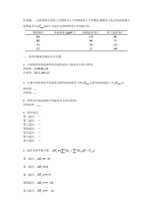
作业题:一过程系统含有的工艺物流为2个热物流和2个冷物流,数据见下表;冷热流股最小传热温差为min T ∆=15℃,试进行还热网络设计及用能评价;物流编号 热容流率CpkW/℃初始温度Ts ℃终了温度Tt ℃H1 150 60 H2 90 55 C1 20 125 C225100一、采用问题表法确定夹点位置:1、分别将所有热流和所有冷流的进出口温度从小到大排列: 热流体:55,60,90,150 冷流体:20,25,100,1252、计算冷热流体的平均温度,即将热流体温度下降min T ∆/2,将冷流体温度上升min T ∆/2: 热流体:,,, 冷流体:,,,3、将所有冷热流体的平均温度从小到大排列: 冷热流体:,,,,,,,4、划分温区: 第一温区: — 第二温区: — 第三温区: — 第四温区: — 第五温区: — 第六温区: — 第七温区: —5、温区内热平衡计算:))((1i +--=∆∑∑i i HCT T CpCp H第一温区:1H ∆== -20 第二温区:2H ∆== 0 第三温区:3H ∆=+= 75 第四温区:4H ∆=+= -120 第五温区:5H ∆=+= -10第六温区:6H ∆=+= 75 第七温区:7H ∆== 106、计算外界无热量输入时各温区之间的热通量: 第一温区:输入热量=0,输出热量=20第二温区:输入热量=20,输出热量=20+0=20 第三温区:输入热量=20,输出热量=20-75=-55 第四温区:输入热量=-55,输出热量=-55+120=65 第五温区:输入热量=65,输出热量=65+10=75 第六温区:输入热量=75,输出热量=75-75=0 第七温区:输入热量=0,输出热量=0-10=107、计算外界输入最小公用工程时各温区之间的热通量: 第一温区:输入热量=55,输出热量=55+20=75 第二温区:输入热量=75,输出热量=75+0=75 第三温区:输入热量=75,输出热量=75-75=0 第四温区:输入热量=0,输出热量=0+120=120 第五温区:输入热量=120,输出热量=120+10=130 第六温区:输入热量=130,输出热量=130-75=55 第七温区:输入热量=55,输出热量=55-10=458、确定夹点位置第三、第四温区之间热通量为0,此处就是夹点,即夹点在平均温度℃,热物流90℃,冷物流75℃处;最小加热公用工程量为55kW,最小冷却公用工程量为45kW;二、使用Aspen Energy Analyzer 设计换热网络:1、 在Aspen Energy Analyzer 中输入冷热物流已知参数,如下图所示:2、 输入冷热物流最小温差为15℃3、 查看夹点计算结果:如上图所示,最小输入热量值为55KJ/h,冷最小冷却热量值为45KJ/h;夹点处温度为热物流90℃,冷物流75℃,与问题表法计算结果相同;4、设计换热方案:由Aspen Energy Analyzer求解换热方案,以下为其中两种推荐方案:三、用能评价:如采用第一种推荐方案,其效果如下:使用热公用工程量为82KJ/h,冷公用工程量为72 KJ/h;分别为最小值的%和%;。
- 1、下载文档前请自行甄别文档内容的完整性,平台不提供额外的编辑、内容补充、找答案等附加服务。
- 2、"仅部分预览"的文档,不可在线预览部分如存在完整性等问题,可反馈申请退款(可完整预览的文档不适用该条件!)。
- 3、如文档侵犯您的权益,请联系客服反馈,我们会尽快为您处理(人工客服工作时间:9:00-18:30)。
6
Heater应用示例 (1)
20℃、0.41MPa、4000 kg/hr 流量的软水在锅 炉中加热成为饱和水蒸气进入生蒸汽总管。求所 需的锅炉供热量。
2.56004E+06Kcal/hr
1000 kg/hr、0.41MPa的饱和水蒸汽用蒸汽过 热器加热到过热度 100℃(0.41MPa),求过热 蒸汽温度和所需供热量。
• 用以表示金属的线径、板厚、管壁厚度,其与毫米之关系如下:
B.W.G 0000 000 00 0 1 2 3 4 5 6 毫米(mm) 11.5 10.8 9.65 8.63 7.62 7.21 6.58 6.04 5.59 5.15 B.W.G 7 8 9 10 11 12 13 14 15 16 毫米(mm) 4.57 4.19 3.76 3.4 3.05 2.77 2.41 2.11 1.83 1.65 B.W.G 毫米(mm)
t m t m,逆
—— 温差修正系数
与冷热两流体温度变化有关,表示为 P 和 R 两参数的函数
f P, R
P
t 2 t 1 冷流体实际温度变化 T 1 t 1 冷流体最大温度变化
T 1 T 2 热流体实际温度变化 R t 2 t 1 冷流体实际温度变化
出口温度或温度变化和下列之一:
压力 热负荷 汽化分率
4
Heater - 连接
Heater 模型的连接图如下:
5
Heater 输入规定
对于单相用压力(压降)和下列之一:
出口温度 热负荷或入口热流股 温度变化
汽化分率为: 1是露点, 0是泡点 简单的例子:
常压下,0℃、1000kg/hr的水升高1 ℃,需要多少热量? (热力学方法使用SRK)
逆流 Countercurrent
并流
Cocurrent
16
HeatX—LMTD校正
常数 Constant
由用户指定校正系数,可查手册。
几何结构
Geometry
由软件根据换热器结构和流动情况计算。
用户子程序 User-subr
17
传热温差:推动力
列管式换热器中两种流体的流动比较复杂的多程流动。 对于错流或折流平均温差,通常是先按逆流求算,然后再根 据流动型式加以修正,即
14
HeatX—计算类型
有两个选项:
简捷计算 Short-cut
• 不考虑换热器的几何结构对传热和压降的影响,人为设 定传热系数和压降。
详细计算
Detailed
• 根据换热器的几何结构和流场情况自动计算传热换热系 数和压降。首先确定热侧—管程/壳程;冷侧—管程/壳程
15
HeatX—流动方向
Aspen Plus 换热过程
2013年8月11日星期日
1
换热器
模型
Heater HeatX MHeatX HXFlux Hetran*
说明
加热器或冷却器 两物流换热器 多物流换热器 对流给热换热器 BJAC Hetran 程 序界面 BJAC Aerotran 程序界面
目的
确定热和相态条件 两股物流的换热器 任何数量物流的换热器 对流换热过程模拟 管壳式换热器的设计和 模拟 空冷器的设计和模拟
用法
换热器、冷却器、阀门、当与功有关 的结果不需要时的泵和压缩机 两股物流换热器、当知道管壳换热器 尺寸时可以进行核算. 多股热流和冷流换热器、两股物流换 热器 、LNG 换热器. 用于计算采用对流换热的热接收器与 热源之间的热传递 具有多种结构的管壳式换热器. 具有多种结构的空冷器. 用于模拟节煤 器和加热炉的对流段.
HeatX 执行:
10
操作 HeatX
HeatX 不能: 进行设计计算 进行机械震动分析 估算污垢系数
11
操作 HeatX
当规定HeatX时,要考虑: 严格/详细计算或 简化/简捷法 什么规定类型 怎样计算
对数平均温差 传热系数 压降
用什么设备和几何尺寸规定
12
HeatX 输入规定
管子排列模式
正方形-90℃ 旋转正方形-45℃ 三角形-30℃ 旋转三角形-60℃
三角形排列比正方形排列更为紧凑,管外流体的湍动程度高,给热系数 大,但正方形排列的管束清洗方便,对易结垢流体更为适用,旋转45 ℃放置,也可提高给热系数。
32
HeatX—几何结构
管子壁厚
管子内径 管壁厚度 伯明翰线规
26
HeatX—应用示例(1)
用1200kg/hr饱和水蒸汽(0.3MPa)加热2000kg/hr甲醇 (20℃、0.3MPa)。离开换热器的蒸汽冷凝水压力为 0.28MPa、过冷度为2℃。换热器传热系数根据相态 选择。求甲醇出口温度、相态、需要的换热面积。 (LMTD校正选用0.95)
热力学方法使用NRTL 109.8℃、气相、9.413m2
245.57℃、51034.7kcal/hr
7
Heater应用示例 (2)
流量为1000kg/hr、0.11MPa、含乙醇70%w、水 30%w的饱和蒸汽在蒸汽冷凝器中部分冷凝,冷凝 物流的汽/液比(摩尔)=1/3。求冷凝器热负荷。
-238597Kcal/hr
流量为100kg/hr、0.2MPa、20℃的丙酮 (CH3COCH3)通过一电加热器。当加热功率分别为 2kW、5kW、10kW和20kW 时,求出口物流的状态。
Heaters(加热器) Coolers(冷却器) Valves(阀门,仅改变压力,不涉及阻力) Pumps (泵)和 Compressors (压缩机)(无论何时 都不需要与功有关的结果。)
3
Heater 输入规定
允许组合: 压力 (或压降) 和下列之一:
出口温度 热负荷或入口热流股 汽化分率 温度变化 过冷或过热度数
Aerotran*
ASPEN Plus 7.0以后改名为Aspen Exchanger Design and Rating
* Requires separate license
2
操作Heater
Heater 模块在规定热力学状态下把多股入口物流 混合生成单股出口物流。 可以使用 Heater 表示:
27
HeatX—详细计算
压降 ( Pressure Drop )
分别指定热侧和冷侧的出口压力 ( Outlet pressure ) 根据几何结构计算 ( Calculated from geometry ) 依据流体关联式计算压降管侧压降 Flow-dependent correlation )
外壳直径:300 mm ,公称面积:10 m2, 管长:3m,管径:Ф19x2mm ,管数:76 ,管心距: 25mm,排列方式:正三角,管程数:2 ,壳程数:1 折流板间距:150 mm ,个数:19 折流板缺口高度:79 mm 壳层接管直径:进口200mm、出口200mm 管程接管直径:进口32mm、出口38mm
(
总传热系数方法 ( U methods )
常数 ( Constant ) 相态法 ( Phase specific values ) 幂函数 ( Power law expression ) 换热器几何结构 ( Exchanger Geometry ) 传热膜系数 ( Film coefficients ) 用户子程序 ( User-subroutine )
17 18 19 20 21 22 23 24 25
1.47 1.24 1.07 0.89 0.81 0.71 0.63 0.56 0.51
33
HeatX—几何结构
折流板结构数据
34
HeatX—应用示例(2)
用1200kg/hr饱和水蒸汽(0.3MPa)加热2000kg/hr甲醇 (20℃、0.3MPa)。离开换热器的蒸汽冷凝水压力为 0.28MPa、过冷度为2℃。换热器传热系数根据相态 选择。求甲醇出口温度、相态、需要的换热面积。 选用下面的数据进行核算:
共 temperature decrease) 有 12 temperature approach) 个 选 degrees subcooling) 项
vapor fraction)
20
HeatX—热物流出口温差
21
HeatX—换热器设定
冷物流出口温度 (Cold stream outlet 冷物流出口温升 (Cold stream outlet 冷物流出口温差 (Cold stream outlet 冷物流出口过热度 (Cold stream outlet 冷物流出口蒸汽分率 (Cold stream outlet temperature)
共 temperature increase) 有 13 temperature approach)个 选 degrees superheat) 项
vapor fraction)
22
HeatX—冷物流出口温差
23
HeatX—换热器设定
热物流出口减冷物流进口温差
(Hot outlet - cold inlet temperature difference) (Hot inlet - cold outlet temperature difference)
热物流进口减冷物流出口温差
热负荷 (Exchanger duty)
共 有 13 个 选 项
24
HeatX—简捷计算
压降( ssure Drop )
分别指定热侧和冷侧的出口压力( Outlet pressure )
• 指定值 > 0,代表出口的绝对压力值 • 指定值 ≤ 0,代表出口相对于进口的压力降低值
选择如下规定之一: 传热面积和几何尺寸 换热负荷 热端或冷端出口物流: